THE STRUCTURE OF THE NUCLEON

These lectures give an introduction to the structure of the nucleon as seen with the electromagnetic probe. Particular emphasis is put on the form factors, the strangeness content, Compton scattering and polarizabilities, pion photo- and electroproduction, the spin structure and sum rules. The existing data are compared to predictions obtained from chiral perturbation theory, dispersion theory and effective Lagrangians.

1 Introduction

Nucleons are composite systems with many internal degrees of freedom. The constituents are quarks and gluons, which are bound by increasingly strong forces if the momentum transfer decreases towards the GeV region. The “running” coupling constant of the strong interaction, $\alpha_{s}(Q^{2})$ in fact diverges if $Q^{2}$ approaches $\Lambda^{2}_{QCD}\approx(200~{}$MeV/c)² corresponding to a scale in space of about 1 fm. This is the realm of nonperturbative quantum chromodynamics (QCD), where confinement plays a major role, and quarks and gluons cluster in color neutral objects. Such correlations between the constituents have the consequence that nucleons in their natural habitat, i.e. at the confinement scale, have to be described by hadronic degrees of freedom rather than quarks and gluons.

QCD is a nonlinear gauge theory developed on the basis of massless quarks and gluons $\!{}^{{\bf?}}$. The interaction among the gluons gives rise to the nonlinearity, and the interaction among the quarks is mediated by the exchange of gluons whose chromodynamic vector potential couples to the vector current of the quarks. If massless particles interact by their vector current, their helicity remains unchanged. In practice one has to restrict this discussion to $u$, $d$ and $s$ quarks with masses $m_{u}\approx 5$ MeV, $m_{d}\approx 9$ MeV and $m_{s}\approx 175$ MeV, which are all small at the mass scale of the nucleon. These quarks can be described by SU(3)${}_{R}\otimes$ SU(3)_L as long as right and left handed particles do not interact, which is what happens if the helicity is conserved. By combining right and left handed currents, one obtains the vector currents $J_{\mu}^{a}$ and the axial vector currents $J_{5\mu}^{a}$,

$$J_{\mu}^{a}=\bar{q}\gamma_{\mu}\frac{\lambda^{a}}{2}q\ ,\ \ \ J_{5\mu}^{a}=\bar{q}\gamma_{\mu}\gamma_{5}\frac{\lambda^{a}}{2}q\ ,$$ (1)

where $q$ are Dirac spinors of the massless and point-like light quarks and $\gamma_{\mu},\gamma_{5}$ the appropriate Dirac matrices. The quantities $\lambda^{a}$, $a=1\ ...\ 8$ denote the Gell-Mann matrices of SU(3) describing the flavor structure of the 3 light quarks. It is often convenient to introduce the unit matrix $\lambda^{0}$ in addition to these matrices.

In the context of these lectures we shall only need the “neutral” currents corresponding to $\lambda=3$, 8 and 0, which have a diagonal form in the standard representation. The photon couples to quarks by the electromagnetic vector current $J_{\mu}^{em}\sim J_{\mu}^{(3)}+\frac{1}{\sqrt{3}}J_{\mu}^{(8)}$, corresponding to isovector and isoscalar interactions respectively. The weak neutral current mediated by the $Z^{0}$ boson couples to the 3rd, 8th and 0th components of both vector and axial currents. While the electromagnetic current is always conserved, $\partial^{\mu}J_{\mu}^{em}=0$, the axial current is only conserved in the limit of massless quarks. In this limit there exist conserved charges $Q^{a}$ and axial charges $Q_{5}^{a}$, which are connected by current algebra,

$$[Q^{a},Q^{b}]=if^{abc}Q^{c}\ ,\ \ [Q^{a}_{5},Q^{b}_{5}]=if^{abc}Q^{c}\ ,\ \ [Q^{a}_{5},Q^{b}]=if^{abc}Q_{5}^{c}\ ,$$ (2)

with $f^{abc}$ the structure constants of SU(3). Such relations were an important basis of low energy theorems (LET), which govern the low energy behavior of (nearly) massless particles.

The puzzle we encounter is the following: The massless quarks appearing in the QCD Lagrangian conserve the axial currents but the nucleons as their physical realizations are massive and therefore do not conserve the axial currents. The puzzle was solved by Goldstone’s theorem. At the same time as the “3 quark system” nucleon becomes massive by means of the QCD interaction, the vacuum develops a nontrivial structure due to finite expectation values of quark-antiquark pairs (condensates $\langle\bar{q}q\rangle$), and so-called Goldstone bosons are created, $\bar{q}q$ pairs with the quantum numbers of pseudoscalar mesons. These Goldstone bosons are massless, and together with the massive nucleons they act such that chirality is locally conserved. This mechanism can be compared to the local gauge symmetry of quantum electrodynamics, which is based on the fact that both (massless) photon and (massive) matter fields have to be gauge transformed.

In QCD the chiral symmetry is definitely broken by the small but finite quark masses. As a consequence also the physical “Goldstone bosons”, in particular the pions, acquire a finite mass $m_{\pi}$, which is generally assumed (though not proven) to follow the Gell-Mann-Oakes-Renner relation

$$m_{\pi}^{2}f_{\pi}=-(m_{u}+m_{d})\langle\bar{q}q\rangle\ ,$$ (3)

with the condensate $\langle\bar{q}q\rangle\approx-(225~{}{\mbox{MeV}})^{3}$, and $f_{\pi}\approx 93~{}$MeV the pion decay constant. Since the pions are now massive, the corresponding axial currents are no longer conserved and the 4-divergence of the axial current becomes

$$\partial^{\mu}J_{5\mu}^{a}\approx-f_{\pi}m_{\pi}^{2}\phi_{\pi}^{a}\ ,$$ (4)

where $\phi_{\pi}^{a}$ describes the local field of charged pions $(a=1$ and 2). In other words the weak decays

$$\pi^{+}\rightarrow\mu^{+}+\nu_{\mu}\ \ \ {\mbox{and}}\ \ \ \pi^{-}\rightarrow\mu^{-}+\bar{\nu}_{\mu}$$ (5)

proceed via coupling to the axial current (Fig. 1).The pion and its axial current disppear from the hadronic world and leave the (hadronic) vacuum behind. In particular we note that a finite value of the divergence of Eq. (4) has 3 requirements: the decay of the pion can take place, the pion mass is finite, and a local pion field exists.

Figure 1: The 4-divergence of the axial current (PCAC) responsible for charged pion decay, and the axial anomaly visualized by an intermediate quark triangle describing neutral pion decay.

While the charged pions decay weakly with a life-time of $2.6\cdot 10^{-8}$ sec, the neutral pion decays much faster, in $8.4\cdot 10^{-17}$ sec, by means of the electromagnetic interaction,

$$\pi^{0}\rightarrow\gamma+\gamma\ .$$ (6)

Again axial current disappears, corresponding to

$$\partial^{\mu}J_{5\mu}^{3}=\frac{\alpha_{fs}}{\pi}\ \vec{E}\cdot\vec{B}\ ,$$ (7)

where $\alpha_{fs}=e^{2}/4\pi$ is the fine structure constant, and $\vec{E}$ and $\vec{B}$ are the electromagnetic fields. We note that two electromagnetic fields have to participate, because two photons are created, and that they have to be combined as a pseudoscalar, because the pseudoscalar pion disappears. The transition of Eq. (7) can be visualized by the intermediate quark triangle of Fig. 1. It is called the “triangle anomaly”, because such transitions cannot exist in classical theories but only occur in quantum field theories via the renormalization procedure. Such terms are also predicted on general grounds (Wess-Zumino-Witten term). We note in passing that a similar anomaly is obtained in QCD by replacing the electromagnetic fields by the corresponding color fields, $\vec{E}_{c}$ and $\vec{B}_{c}$, $\alpha_{fs}$ by the strong coupling $\alpha_{s}$, and by an additional factor 3 for u, d, and s quarks,

$$\partial^{\mu}J_{5\mu}^{0}=3\ \frac{\alpha_{s}}{\pi}\ \vec{E}_{c}\cdot\vec{B}_{c}\ .$$ (8)

As a consequence the component $J_{5\mu}^{0}$ is not conserved, not even in the case of massless quarks (“$U_{A}(1)$ anomaly”).

Unfortunately, no ab-initio calculation can yet describe the interesting but complicated world of the confinement region. In principle, lattice gauge theory should have the potential to describe QCD directly from the underlying Lagrangian. However, these calculations have yet to be restricted to the “quenched approximation”, i.e. initial configurations of 3 valence quarks. This is a bad approximation for light quarks, because the Goldstone mechanism creates plenty of sea quarks, and therefore the calculations are typically performed for massive quarks, $m_{q}\approx 100$ MeV, and then extrapolated to the small $u$ and $d$ quark masses. In this way one obtains reasonable values for mass ratios of hadrons and qualitative predictions for electromagnetic properties. However, some doubt may be in order whether such procedure will describe the typical threshold behavior of pionic reactions originating from the Goldstone mechanism.

A further “ab initio” calculation is chiral perturbation theory (ChPT), which has been established by Weinberg in the framework of effective Lagrangians and put into a systematic perturbation theory by Gasser and Leut-wyler $\!{}^{{\bf?}}$. Based on the Goldstone mechanism, the threshold interaction of pions is weak both among the pions and with nucleons, and furthermore the pion mass is small and related to the small quark masses $m_{u}$ and $m_{d}$ by Eq. (3). As a consequence ChPT is a perturbation in a parameter $p:=(p_{1},p_{2},...;m_{u},m_{d})$, where $p_{i}$ are the external 4-momenta of a particular (Feynman) diagram. (Note that also the time-like component, the energy, is small at threshold because of the small mass!). This theory has been applied to photoinduced reactions by Bernard, Kaiser, Meißner and others $\!{}^{{\bf?}}$ over the past decade. As a result several puzzles have been solved and considerable insight has been gained. There exists, however, the problem that ChPT cannot be renormalized in the “classical” way by adjusting a few parameters to the observables. Instead the renormalization has to be performed order by order, the appearing infinities being removed by counter terms. This procedure gives rise to a growing number of low energy constants (LECs) describing the strength of all possible effective Lagrangians consistent with QCD, at any given order of the perturbation series. These LECs, however, cannot (yet) be derived from QCD but have to be fitted to the data, which leads to a considerable loss of predictive powers in the higher orders of perturbation. A further problem arises in the nucleonic sector due to the nucleon’s mass $M$, which is of course not a small expansion parameter. The latter problem has been overcome by heavy baryon ChPT (HBChPT), a kind of Foldy-Wouthuysen expansion in $M^{-1}$. The solution is achieved, however, at the expense of going from an explicitly relativistic field theory to a nonrelativistic scheme.

Beside lattice gauge theory and ChPT, which are in principle directly based on QCD, there exists a host of QCD inspired models, which we shall not discuss at this point but occasionally refer to at later stages.

2 KINEMATICS

Let us consider the kinematics of the reaction

$$e(k_{1})+N(p_{1})\rightarrow e(k_{2})+N(p_{2})\ ,$$ (9)

with $k_{1}=(\omega_{1},\vec{k}_{1})$ and $p_{1}=(E_{1},\vec{p}_{1})$ denoting the four-momenta of an electron $e$ and a nucleon $N$ in the initial state, and corresponding definitions for the final state (Fig. 2). These momenta fulfil the on-shell conditions

$$p_{1}^{2}=p_{2}^{2}=M^{2}\ ,\ \ \ k_{1}^{2}=k_{2}^{2}=m^{2}\ ,$$ (10)

and furthermore conserve total energy and momentum,

$$k_{1}+p_{1}=k_{2}+p_{2}\ .$$ (11)

Figure 2: The reaction $k_{1}+p_{1}\rightarrow k_{2}+p_{2}$. The 4-momenta $p_{1}$ and $p_{2}$ describe a nucleon in the initial and final states respectively, while $k_{1}$ and $k_{2}$ stand for a lepton.

If we also assume parity conservation, the scattering amplitudes should be Lorentz invariants depending on the Lorentz scalars that can be constructed from the four-momenta. By use of Eqs. (10) and (11) it can be shown that there exist only two independent Lorentz scalars, corresponding to the fact that the kinematics of Eq. (9) is completely described by, e.g., the lab energy of the incident electron, $\omega_{L}$, and the scattering angle $\Theta_{L}$. In order to embed relativity explicitly, it is useful to express the amplitudes in terms of the 3 Mandelstam variables

$$s=(k_{1}+p_{1})^{2}\ \ ,\ \ t=(k_{2}-k_{1})^{2}\ \ ,\ \ u=(p_{2}-k_{1})^{2}\ .$$ (12)

Since only two independent Lorentz scalars exist, these variables have to fulfil an auxiliary condition, which is

$$s+t+u=2\ (m^{2}+M^{2})\ .$$ (13)

In the $cm$ frame, the 3-momenta of the particles cancel and $s=(\omega_{cm}+E_{cm})^{2}=W_{s}^{2}=W^{2}$, where $W$ is the total energy in that frame. Furthermore, the initial and final energies of each particle are equal, hence $t=-(\vec{k}_{2}-\vec{k}_{1})^{2}_{cm}=-\vec{q}\ ^{2}_{cm}$, where $\vec{q}_{cm}$ is the 3-momentum transfer in the $cm$ system. From these definitions it follows that $s\geq(m+M)^{2}$ and $t\leq 0$ in the physical region. Since $s$ is Lorentz invariant, the threshold energy $\omega_{lab}$ can be obtained by comparing $s$ as expressed in the $lab$ and $cm$ frames. Moreover, in a general frame $t=(k_{2}-k_{1})^{2}=q^{2}<0$ describes the square of 4-momentum of the virtual photon $\gamma^{\ast}$, exchanged in the scattering process (“space-like photon”). Since $t$ is negative in the physical region of electron scattering, we shall define the positive number $Q^{2}=-q^{2}$ for further use. We also note that in pair annihilation, $e^{+}e^{-}\rightarrow\gamma^{\ast}$, the square of 4-momentum is positive, $q^{2}=m_{\gamma^{\ast}}^{2}>0$ (“time-like photon”).

The above equations can be easily applied to Compton scattering,

$$\gamma(k_{1})+N(p_{1})\rightarrow\gamma(k_{2})+N(p_{2})\ ,$$ (14)

by replacing $m$ by zero, the mass of a real photon, and to virtual Compton scattering (VCS),

$$\gamma{\ast}(k_{1})+N(p_{1})\rightarrow\gamma(k_{2})+N(p_{2})\ ,$$ (15)

by replacing $m^{2}\rightarrow k_{1}^{2}=q^{2}<0$. Due to the spins of photon and nucleon, several Lorentz structures appear in the scattering amplitude, and each of these structures has to be multiplied by a scalar function depending in the most general case on 3 variables, $F=F(s,t,Q^{2})$.

Another generalization occurs if the nucleon is excited in the scattering process, in which case $p_{2}^{2}=(M^{\ast})^{2}>M^{2}$ becomes an additional variable. Introducing the Bjorken variable $x=Q^{2}/2p_{1}\cdot q$ we find that $x=1$ corresponds to elastic scattering, while inelastic scattering is described by values $0\leq x<1$.

Figure 3: The Mandelstam plane for Compton scattering, with the crossing symmetrical variable $\nu=(s-u)/4M$ and $t$ as orthogonal coordinates. The horizontally hatched areas are the physically allowed regions for s, t, and u channel kinematics. The scattering amplitudes become complex if particle production is allowed, i.e. for $t\geq 4m_{\pi}^{2}$, and $s$ or $u\geq(M+m_{\pi})^{2}$. As a consequence the scattering amplitudes are real inside the triangle formed by the dashed lines near the origin.

For further use we shall acquaint ourselves with the Mandelstam plane for (real) Compton scattering, as shown by Fig. 3. Due to the symmetry of the Mandelstam variables, the figure can be constructed on the basis of a triangle with equal sides and heights equal to $2M^{2}$ according to Eq. (13) for $m=m_{\gamma}=0$. The axes $s=0$, $t=0$, and $u=0$ are then obtained by drawing straight lines through the sides of the triangle. The physically allowed region for $k_{1}+p_{1}\rightarrow k_{2}+p_{2}$ is given by the horizontally hatched area called “s channel” with $s\geq M^{2}$ and $t\leq 0$. If we replace $p_{1}\rightarrow-p_{1}$ and $p_{2}\rightarrow-p_{2}$ in Eq. (11), we obtain the “u channel” reaction $k_{1}+p_{2}\rightarrow k_{2}+p_{1}$ given by the horizontally hatched area to the left.

Figure 4: The pole terms contributing to Compton scattering. From left to right on the $rhs$ the direct nucleon pole term, the crossed nucleon pole term, and the $\pi^{0}$ pole term.

Finally, if we look at Fig. 2 from the left side, we obtain the $t$ channel reaction $\gamma(k_{1})+\gamma(-k_{2})\rightarrow N(p_{1})+\bar{N}(-p_{2})$, which corresponds to the replacements $k_{2}\rightarrow-k_{2}$ and $p_{1}\rightarrow-p_{1}$ and is physically observable for $t>2M^{2}$ (hatched area at top of Fig. 3). Referring again to the $s$ channel, the boundaries of the physical region correspond to the scattering angles 0 and 180^∘. The former case leads to zero momentum transfer, i.e. the line $t=0$, the latter case to the hyperbolic boundary of the region at negative $t$ values. The u-channel region is then simply obtained by a reflection of the figure at the line $s=u$ given by the $t$ axis. Finally, the boundary of the t-channel region is given by the upper branch of the hyperbola, separated from the lower one by $4M^{2}$.

Still in the context of Compton scattering, Fig. 4 shows the Born diagrams (tree graphs) contributing to the reaction. In order of appearance on the $rhs$, we find the direct, the crossed, and the $\pi^{0}$ pole terms, exhibiting pole structures as $(s-M^{2})^{-1}$, $(u-M^{2})^{-1}$ and $(t-m_{\pi}^{2})^{-1}$ respectively. Except for the origin at $s=u=M^{2}$ (“scattering” of photons with zero momentum), these poles are situated on straight lines outside of the physical regions. However, photon scattering at small energies is obviously dominated by the poles at $s=M^{2}$ and $u=M^{2}$. The “low-energy theorem” asserts that for a particle with charge $e$ and mass $M$, the scattering amplitude behaves as $T=-\frac{e^{2}}{M}+O(\omega_{cm}^{2})$, where $e^{2}/4\pi\approx 1/137$. It is derived on the basis that (i) only the Born terms have pole singularities for $\omega_{cm}\rightarrow 0$, which results in the Thomson amplitude $(-e^{2}/M)$, and (II) gauge invariance or current conservation, which allows one to express the next-to-leading-order terms in $\omega_{cm}$ by the Born contributions. Therefore, the internal structure (polarizability) of the system enters only in terms of relative order $\omega_{cm}^{2}$, i.e. is largely suppressed near threshold.

If the energy of the photon is sufficient to produce a pion, $\sqrt{s}>M+m_{\pi}$, Compton scattering competes with the much stronger hadronic reactions and becomes complex. The same is true in the $t$ channel, whenever the two photons carry more energy than $\sqrt{t}=2m_{\pi}$. Therefore the Compton amplitudes are only real in an area around the origin $(s=u=M^{2},\ t=0)$, i.e. in the triangle shaped by the dashed lines in Fig. 3. Due to this reality relation, however, the Compton amplitudes can be analytically continued into the unphysical region, and information from the different physical regions can be combined to construct a common amplitude for the whole Mandelstam plane. Summarizing the role of the singularities for the specific reaction of Compton scattering we find: (I) The nucleon poles in the direct and crossed Born graphs, at $s=M^{2}$ and $u=M^{2}$, which are close to and therefore important near threshold, (II) the pion pole term at $t=m_{\pi}^{2}$ and a branch cut starting at $t=4m_{\pi}^{2}$ due to the opening of the $2\pi$ continuum, which affect the forward amplitude at any energy and (III) the opening of hadronic channels at $s,u>(M+m_{\pi})^{2}$, which lead to a complex amplitude and a much enhanced Compton cross section, particularly near resonances at $s=M_{\mbox{\scriptsize{res}}}^{2}$.

Let us finally consider the spin degrees of freedom of the involved particles. A virtual photon with momentum $\vec{q}$ carries a polarization described by the vector potential $\vec{A}$, which has both a transverse part, $\vec{A}_{T}\perp\vec{q}$, as in the case of a real photon, and a longitudinal component $\hat{q}\cdot\vec{A}$, which is related to the time-like component $A_{0}$ by current conservation, $q\cdot A=q_{0}A_{0}-\vec{q}\cdot\vec{A}=0$. As a consequence the cross section for the reaction of Eq. (9) takes the (somewhat symbolical) form

$$\frac{d\sigma}{d\Omega}=\Gamma(\sigma_{T}+\varepsilon\sigma_{L})\ ,$$ (16)

where $\Gamma$ describes the flux of the virtual photon spectrum, and $\sigma_{T}$ and $\sigma_{L}$ the transverse and longitudinal cross sections respectively. The so-called transverse polarization $\varepsilon$ of the virtual photon field is given by kinematical quantities only, which can be varied such that the partial cross sections remain constant. In this way the two partial cross sections can be separated by means of a “Rosenbluth plot”.

Concerning the electron, we shall assume that it is highly relativistic, hence its spin degree of freedom will be described by the helicity $h=\vec{s}\cdot\hat{k}=\pm\frac{1}{2}$, the projection of the spin $\vec{s}$ on the momentum vector $\vec{k}$. As long as the interaction is purely electromagnetic, a polarization of the electron alone does not change the structure of the cross section, Eq. (16). However, new structures appear if both electron and nucleon are polarized. In particular the reaction $\vec{e}+\vec{N}\rightarrow$ anything is described by the cross section $\!{}^{{\bf?}}$

$$\frac{d\sigma}{d\Omega}=\Gamma[\sigma_{T}+\varepsilon\sigma_{L}+P_{e}P_{x}\sqrt{2\varepsilon(1-\varepsilon)}\ \sigma^{\prime}_{LT}+P_{e}P_{z}\sqrt{1-\varepsilon^{2}}\ \sigma^{\prime}_{TT}]\ ,$$ (17)

where $P_{e}=2h=\pm 1$ refers to the helicity of the electron, and $P_{z}$ and $P_{x}$ are the longitudinal and transverse polarizations of the nucleon defined by the momentum of the virtual photon and an axis perpendicular to that direction (note: $P_{x}$ lies in the scattering plane of the electron and takes positive values on the side of the scattered electron).

In a more general experiment with production of pseudoscalar mesons, e.g. pions,

$$\vec{e}+\vec{N}\rightarrow e^{\prime}+N^{\prime}+\pi\ ,$$ (18)

up to 18 structure functions can be defined $\!{}^{{\bf?}}$, and this number increases further when higher spins are involved, e.g. if the electron is scattered on a deuteron target or if a vector particle (real photon, $\rho$ or $\omega$ meson etc.) is produced.

3 FORM FACTORS

Consider the absorption of a virtual photon with four-momentum q at an hadronic vertex. If the hadron stays intact after this process, i.e. in the case of elastic lepton scattering, the photon probes the expectation value of the hadronic vector current. If moreover the hadron is a scalar or pseudoscalar particle, the vector current has to be proportional to the two independent combinations of the 3 external four-momenta. Choosing $q=p_{2}-p_{1}$ and $P=(p_{1}+p_{2})/2$ as the independent vectors,

$$J_{\mu}:=\langle p_{2}\mid J_{\mu}\mid p_{1}\rangle=F_{1}\frac{P_{\mu}}{m}+F_{2}\frac{q_{\mu}}{m}\ .$$ (19)

In this way we define two form factors, $F_{1}$ and $F_{2}$, which have to be scalars and as such may be expressed by functions of the independent Lorentz scalars that can be constructed. It is again a simple exercise to show that there exists only one independent scalar, e.g. $Q^{2}=-q^{2}$, because $P\cdot q=0$ and $P^{2}=m^{2}-\frac{1}{4}q^{2}$ in the case of elastic scattering off a particle with mass $m$.

Next we can exploit the fact that the vector current of Eq. (19) is conserved, which follows from gauge invariance. The result is

$$0=q_{\mu}J^{\mu}=F_{1}\frac{p_{2}^{2}-p_{1}^{2}}{2m}+F_{2}\frac{q^{2}}{m}\ .$$ (20)

Since $p_{1}^{2}=p_{2}^{2}=m^{2}$ for on-shell particles, the first term is zero and hence $F_{2}$ has to vanish identically. Therefore the vector current of, e.g., an on-shell pion has to take the form

$$J^{\mu}(\pi)=\frac{p_{1}^{\mu}+p_{2}^{\mu}}{2m_{\pi}}\ F_{\pi}(Q^{2})\ .$$ (21)

The form factor is normalized to $F_{\pi}(0)=e_{\pi}$, here and in the following in units of the elementary charge e. In this way we obtain, in the static limit $q_{\mu}\rightarrow 0$ and $p_{2\mu}\rightarrow p_{1\mu}\Rightarrow(m_{\pi},\vec{0})$, the result $J_{\mu}\Rightarrow(e_{\pi},\vec{0})$ for a charge $e_{\pi}$ at rest.

The situation is more complicated in the case of a particle with a spin like the nucleon, because now the independent momenta $q$ and $P$ can be combined with the familiar 16 independent $4\times 4$ matrices of Dirac’s theory: 1 (scalar), $\gamma_{5}$ (pseudoscalar), $\gamma_{\mu}$ (vector), $i\gamma_{5}\gamma_{\mu}$ (axial vector), and $\sigma_{\mu\nu}$ (antisymmetrical tensor). It is straightforward but somewhat tedious to show that the most general vector current of a spin-1/2 particle has to take the form

$$J_{\mu}:=\langle p_{2}\mid J_{\mu}\mid p_{1}\rangle=\bar{u}_{p_{2}}\left(F_{1}\gamma_{\mu}+i\frac{F_{2}}{2m}\sigma_{\mu\nu}q^{\nu}\right)u_{p_{1}}\ ,$$ (22)

where $u_{p1}$ and $u_{p2}$ are the 4-spinors of the nucleon in the initial and final states respectively. The first structure on the $rhs$ is the Dirac current, which appears with the Dirac form factor $F_{1}$. The second term reflects the fact that due to its internal structure the particle acquires an anomalous magnetic moment $\kappa$, which appears with the Pauli form factor $F_{2}$. These form factors are normalized to $F_{1}^{p}(0)=1$, $F_{2}^{p}(0)=\kappa_{p}=1.79$ and $F_{1}^{n}(0)=0$, $F_{2}^{n}(0)=\kappa_{n}=-1.91$ for proton and neutron respectively.

From the analogy with nonrelativistic physics, it is seducing to associate the form factors with the Fourier transforms of charge and magnetization densities. The problem is that a calculation of the charge distribution $\rho(\vec{r})$ involves a 3-dimensional Fourier transform of the form factor as function of $\vec{q}$, while in general the form factors are functions of $Q^{2}=\vec{q}\ ^{2}-\omega^{2}$. However, there exists a special Lorentz frame, the Breit or brickwall frame, in which the energy of the virtual photon vanishes. This can be realized by choosing, e.g., $\vec{p}_{1}=-\vec{q}\ /2$ and $\vec{p}_{2}=+\vec{q}\ /2$ leading to $E_{1}=E_{2}=(m^{2}+\vec{q}\ ^{2}/4)^{1/2}$, $\omega=0$, and $Q^{2}=\vec{q}\ ^{2}$.

In that frame the vector current takes the form

$$J_{\mu}=\left(G_{E}(Q^{2})\ ,\ i\frac{\vec{\sigma}\times\vec{q}}{2m}G_{M}(Q^{2})\right)\ ,$$ (23)

where $G_{E}$ stands for the time-like component of $J_{\mu}$ and hence is identified with the Fourier transform of the electric charge distribution, while $G_{M}$ appears with a structure typical for a static magnetic moment and hence is interpreted as Fourier transform of the magnetization density. The two “Sachs form factors” $G_{E}$ and $G_{M}$ are related to the Dirac form factors by $\!{}^{{\bf?}}$

$$G_{E}(Q^{2})=F_{1}(Q^{2})-\tau F_{2}(Q^{2})\ ,\ \ \ G_{M}(Q^{2})=F_{1}(Q^{2})+F_{2}(Q^{2})\ ,$$ (24)

where $\tau=Q^{2}/4m^{2}$ is a measure of relativistic (recoil) effects. While Eq. (24) is taken as a general, covariant definition, the Sachs form factors can only be Fourier transformed in a special frame, namely the Breit frame, with the result

$$G_{E}(\vec{q}\ ^{2}) = \int\rho(\vec{r})e^{i\vec{q}\cdot\vec{r}}d^{3}\vec{r}$$ (25)

$$= \int\rho(\vec{r})d^{3}\vec{r}-\frac{\vec{q}\ ^{2}}{6}\int\rho(\vec{r})\vec{r}\ ^{2}d^{3}\vec{r}+\ ...\ ,$$

where the first integral yields the total charge in units of $e$, i.e. 1 for the proton and 0 for the neutron, and the second integral defines the square of the electric $rms$ radius, $\langle r^{2}\rangle_{E}:=r_{E}^{2}$ of the particle. The interpretation of $G_{E}$ in terms of the charge distribution has recently been discussed again $\!{}^{{\bf?}}$.

We note that each value of $Q^{2}$ requires a particular Breit frame. Therefore, information has to be compiled from an infinity of different frames, which is then used as input for the Fourier integral for $\rho(\vec{r})$ in terms of $G_{E}(\vec{q}\ ^{2})$. Therefore, the density $\rho(\vec{r})$ is not an observable that we can “see” in any particular Lorentz frame but only a mathematical construct in analogy to a “classical” charge distribution. The problem is, of course, that due to the small mass of an “elementary” particle, recoil effects (measured by $\tau$) and size effects (measured by $\langle r^{2}\rangle$) become comparable and cannot be separated in a unique way. This situation is numerically quite different in the case of a heavy nucleus for which the size effects dominate the recoil effects by many orders of magnitude!

The two Sachs form factors may be determined from the differential cross section

$$\frac{d\sigma}{d\Omega}=\sigma_{\scriptscriptstyle{\mbox{Mott}}}\left(\frac{G_{E}^{2}+\tau G_{M}^{2}}{1+\tau}+2\tau\tan^{2}\frac{\theta}{2}G_{M}^{2}\right)$$ (26)

by means of a “Rosenbluth plot”, showing the cross section as function of $\tan^{2}\frac{\theta}{2}$ for constant $Q^{2}$. The data should lie on a straight line with a slope $2\tau G_{M}^{2}$, and the extrapolation to $\tau=0$ will determine the electric form factor $G_{E}$. Unfortunately, the Rosenbluth plot has a limited range of applicability. For decreasing $Q^{2}$, also $\tau$ and the slope become small and the error bars on $G_{M}^{2}$ increase. Large $Q^{2}$, on the other hand side, lead to a small electric contribution $\sim G_{E}^{2}/\tau$ with large errors for the electric form factor.

Figure 5: The Sachs form factors of neutron and proton as functions of $Q^{2}$, normalized to the dipole ($G_{D}$) and “Platchkov” ($G_{P}$) form factors defined in Eq. (28). The solid and dashed lines are obtained from a fit to the world data, based on dispersion relations. See Ref. $\!{}^{{\bf?}}$ for more details.

In the case of the proton, the Rosenbluth plot was evaluated up to $Q^{2}=8.8$ GeV² at SLAC $\!{}^{{\bf?}}$. The results are shown in Fig. 5. Additional and more precise information can be obtained at the new electron accelerators by double-polarization experiments, in particular by target polarization $\vec{p}(\vec{e},e^{\prime})p$ and recoil polarization, $p(\vec{e},e^{\prime})\vec{p}$. The asymmetry $A$ measured by such an experiment is given by $\!{}^{{\bf?}}$

$$A=-P_{e}\frac{\sqrt{2\tau\varepsilon(1-\varepsilon)}\ G_{E}G_{M}P_{x}+\tau\sqrt{1-\varepsilon^{2}}\ G_{M}^{2}\ P_{z}}{\varepsilon\ G_{E}^{2}+\tau\ G_{M}^{2}}\ ,$$ (27)

where $P_{e}$ is the (longitudinal) polarization of the incident electron, and $P_{x}$ and $P_{z}$ are the transverse and longitudinal polarization components of the nucleon as defined in Eq. (17). In particular we find that the longitudinal-transverse interference term, appearing if the nucleon is polarized perpendicularly (sideways) to $\vec{q}$, will be proportional to $G_{E}G_{M}$, while the transverse-transverse interference term, appearing for polarization in the $\vec{q}$ direction, will be proportional to $G_{M}^{2}$. The ratio of both measurements then determines $G_{E}/G_{M}$ with high precision, because most normalization and efficiency factors will cancel.

Within the large error bars of the experiments, the older data followed surprisingly close the so-called “dipole fit” for the Sachs form factors,

$$G_{E}^{p} = G_{M}^{p}/\mu_{p}=G_{M}^{n}/\mu_{n}=(1+Q^{2}/M_{V}^{2})^{-2}:=G_{D}$$

$$G_{E}^{n}/\mu_{n} = \tau(1+Q^{2}/M_{V^{\prime}}^{2})^{-1}(1+Q^{2}/M_{V}^{2})^{-2}:=G_{P}\ ,$$ (28)

with $\mu_{p}=2.79,\ \mu_{n}=-1.91$, $M_{V}=840$ MeV and $M_{V^{\prime}}=790$ MeV. Since $\tau=Q^{2}/4m^{2},\ G_{E}^{n}(0)$ vanishes, while $G_{E}^{p}(0)=1$ and the magnetic form factors approach the total magnetic moments for $Q^{2}\rightarrow 0$. In the asymptotic region $Q^{2}\rightarrow\infty$, all Sachs form factors should have a $Q^{-4}$ behavior according to perturbative QCD. Inverting Eq. (24) we also find the asymptotic behavior of the Dirac form factors as required by pQCD, $F_{1}\rightarrow Q^{-4}$ and $F_{2}\rightarrow Q^{-6}$.

Already the SLAC experiments showed, however, that $G_{M}^{p}/\mu_{p}G_{D}$ falls much below unity at the higher momentum transfers $\!{}^{{\bf?}}$, reaching values of about 0.65 at $Q^{2}=20$ (GeV/c)². For the reason pointed out before, $G_{E}^{p}$ was not well determined by these experiments. This situation has changed dramatically by the recent results from Jefferson Lab, which were obtained by scattering polarized electrons in coincidence with the polarization of the recoiling protons $\!{}^{{\bf?}}$. In this way it was possible to separate the form factors up to $Q^{2}=3.5$(GeV/c)², where $G_{E}^{p}/G_{M}^{p}$ reaches the surprisingly low value of about 0.55, i.e. $G_{E}^{p}$ falls below $G_{D}$ even faster than $G_{M}^{p}$.

Figure 6: The electric Sachs form factor for the neutron, $G_{E}^{n}$, as function of $Q^{2}$. The dashed line follows the Saclay data, the full line fits the new double-polarization experiments at Mainz. See Ref. $\!{}^{{\bf?}}$ and text for details.

However, the situation is even more complex in the case of the neutron. The only exact information used to be the electric neutron radius, $\langle r^{2}\rangle_{E}^{n}\approx-0.11$ fm², which was obtained by scattering low energy neutrons off a ${}^{208}Pb$ target $\!{}^{{\bf?}}$. Since there is no free neutron target, electron scattering data have to be obtained from light nuclei such as ²H or ³He making appropriate corrections for binding effects. This is a particularly difficult task for $G_{E}^{n}$, because it is smaller than the other form factors by a factor 10-20. In the past, results were obtained by either deuteron breakup in quasifree (neutron) kinematics $\!{}^{{\bf?}}$ or elastic scattering off the deuteron $\!{}^{{\bf?}}$, assuming that all other form factors and wave function corrections were well under control. Though the data reached a remarkable statistical accuracy, large systematical errors remained, particularly with regard to the nucleon-nucleon potential. While it had been pointed out long ago that double-polarization experiments should be much less model-dependent, such data were only taken very recently $\!{}^{{\bf?}}$. As shown in Fig. 6 the electric form factor of the neutron seems to be much larger than previously thought of. With the exception of the ³He point at $Q^{2}\approx 0.35$ (GeV/c)², the new data follow the full line (“Mainz fit”) as opposed to the dashed line (“Saclay fit”, obtained from elastic $ed$ scattering). It is remarkable that the ²H data point at the lowest $Q^{2}$ has moved upward by nearly a factor of 2 by taking account of final state interactions $\!{}^{{\bf?}}$, while these corrections are only at the percent level for the higher $Q^{2}$. This observation is at variance with the earlier assumption that final state interactions would not play any role in this kind of experiment. In view of this lesson from the deuteron it may be assumed that also the lowest ³He data point will move once a complete calculation of final state and meson exchange effects exists.

The following Fig. 7 compares the neutron charge density obtained by Fourier transforming the older and the more recent data. Both results are in qualitative agreement with our expectation that the neutron charge density should have a positive core surrounded by a negative cloud $\!{}^{{\bf?}}$. The remarkable facts are, however, that the new data lead to a lower zero-crossing at r=0.7 fm in comparison with the older results (r=0.9 fm), and that both maximum and minimum become more pronounced. If one naively interprets the total negative charge as the pion cloud, one finds a probability of about 60 % that the neutron has a proton core surrounded by a $\pi^{-}$ cloud. Such an idea is quite natural for models of pions and nucleons, in particular for chiral bag models. It is interesting to note that a similar density is also predicted by the constituent quark model. The hyperfine interaction leading to the $\Delta$-nucleon mass splitting predicts, at the same time, a stronger repulsion of quarks with equal flavor. Therefore the two $d$ quarks with total charge $-2/3$ will move to the bag surface while the up quark goes to the center.

Figure 7: The density distribution of the neutron, $\rho_{E}^{n}=\rho$, as function of the radius $r$. The two lines are the Fourier transforms of the corresponding fits in Fig. 6. Results from Ref. $\!{}^{{\bf?}}$.

Table 1: The proton charge radius $r_{E}^{p}=r_{E}$ derived from various experiments and from a fit based on dispersion theory. Also shown is the radius of an equivalent homogeneous sphere ($R_{eq})$ and the volume Vol of that sphere. See text for details.

	$r_{E}/$fm	$R_{eq}/$fm	Vol/fm3
Stanford $\!{}^{{\bf?}}$	0.81	1.05	4.85
disp. theory $\!{}^{{\bf?}}$	0.85	1.10	5.58
Mainz $\!{}^{{\bf?}}$	0.86	1.11	5.73
opt. and rf. exp. $\!{}^{{\bf?}}$	0.92	1.19	7.06

A final remark is in order concerning the proton radius. The experimental situation for $r_{E}^{p}$ is shown in Table 1. The large data spread for this very elementary quantity is truly surprising. The recent optical and radio frequency experiments had in mind, of course, to search for the limits of quantum electrodynamics by measuring Lamb shifts and hyperfine structures. In spite of an astounding accuracy of about 12 decimals, the analysis was stopped at about the 7th decimal by the existing uncertainties in the proton radius. If all deviations from theory are attributed to size effects, considerably larger radii are obtained than in the case of electron scattering.

The size of the nucleon is not just an academical question, but of tremendous consequence for our understanding of hadronic matter. The Table also shows the radius of an equivalent, homogeneous charge distribution, $R_{eq}=(\frac{5}{3}r_{E}^{2})^{1/2}$, and the resulting “volume” of a nucleon. Obviously the volume grows by nearly 50 % by going from the Stanford value to the more recent results. Hence nucleons in a nucleus may get into a very uncomfortable environment: they need more space than is actually available. This situation is of course quite different from most models of nuclei and nuclear matter, which are based on effective interactions between point particles.

Note added in proof: In a recent paper Rosenfelder pointed out that Coulomb corrections will increase the proton radius, as measured by electron scattering, to $r_{E}=(0.880\pm 0.015)$ fm, with an error bar depending on the fit strategy $\!{}^{{\bf?}}$.

4 STRANGENESS

The strangeness content of the nucleon manifests itself by matrix elements $<N\mid\bar{s}\ \Gamma\ s\mid N>$, with $\Gamma$ any of the 5 Dirac structures of Section 3. Though observation of these matrix elements is necessarily proof for the existence of $s$ quarks in the nucleon, the strength of the 5 matrix elements may well be different. Since there exists no net strangeness in the nucleon, these observables open, in principle, a clear window on sea degrees of freedom. Information on the strange quark content comes essentially from three sources:

1. Deep inelastic lepton scattering.
   The experiments clearly indicate a break-down of the Ellis-Jaffe sum rule based on SU(3) symmetry $\!{}^{{\bf?}}$. Such experiments have led to the so-called “spin crisis” of the nucleon, which was eventually explained by sea quark and gluon contributions to the spin of the nucleon. The observed symmetry breaking is proportional to the axial vector current carried by the $s$ quarks $\!{}^{{\bf?}}$.

2. Pion-nucleon scattering.
   Dispersion analysis allows one to extrapolate $\pi N$ scattering to the (unphysical) Cheng-Dashen point at $s=u$ and $t=2m_{\pi}^{2}$. The scattering amplitude at this point is essentially given by the $\sigma$ term $\!{}^{{\bf?}}$,

   $$\sigma_{\pi N}=\frac{m_{u}+m_{d}}{2}<N\mid\bar{u}u+\bar{d}d\mid N>\ .$$ (29)

   In combination with similar information on $KN$ scattering and approximate SU(3), the scalar $\bar{s}s$ condensate can be determined. The size of this effect is, unfortunately, not well established. The prediction of ChPT is $\!{}^{{\bf?}}$

   $$\sigma_{\pi N}=58.3\ (1-0.56+0.33)\ {\mbox{MeV}}=45\ {\mbox{MeV}}\ ,$$ (30)

   the 3 terms in this equation indicating the (slow) convergence of the perturbation series, while typical phenomenological analyses are in the range of $\sigma_{\pi N}=(60\pm 20)$ MeV. It is obvious that this uncertainty will also affect the value of the strangeness contribution, which therefore carries large error bars,

   $$y=\frac{2<\bar{s}s>}{<\bar{u}u+\bar{d}d>}=0.21\pm 0.20\ .$$ (31)

3. Parity-violating lepton scattering.
   The interest in this experiment stems from the observation that the photon and the $Z^{0}$ gauge boson couple differently to the vector currents of the quarks. An interference term of the electromagnetic and the weak neutral current is parity-violating (PV) and thus can be determined by a PV asymmetry. This presents the opportunity to measure a third form factor, in addition to the electromagnetic form factors of neutron and proton. If these 3 form factors would be known to sufficient precision, the density distributions of $u,\ d$ and $s$ quarks could be determined $\!{}^{{\bf?}}$.

The strange vector current $<N^{\prime}\mid\bar{s}\gamma_{\mu}s\mid N>$ takes the general form of Eq. (22) with Dirac $(F_{1}^{s})$ and Pauli $(F_{2}^{s})$ strangeness form factors. Since the nucleon has no net strangeness, $F_{1}^{s}(Q^{2}=0)=0$. It follows from Eq. (24) that

$$G_{E}^{s}(Q^{2}) = -\frac{1}{6}Q^{2}<r^{2}>_{E}^{s}+[Q^{4}]\ ,$$

$$G_{M}^{s}(Q^{2}) = \mu^{s}+[Q^{2}]\ ,$$ (32)

with $<r^{2}>_{E}^{s}$ the square of the electric $rms$ radius and $\mu^{s}=\kappa^{s}=F_{2}^{s}(0)$ the (anomalous) magnetic moment due to the strange quark sea. Instead of the radius one often finds the dimensionless quantity $\varrho^{s}=dG/d\tau$, the derivative of a particular form factor with regard to the quantity $\tau$, which is related to

$$<r^{2}>^{s}=-0.066\ {\mbox{fm}}^{2}\ \varrho^{s}\ .$$ (33)

The new information from parity-violating $\vec{e}+N\rightarrow e^{\prime}+N^{\prime}$ can be obtained from the asymmetry $A=(d\sigma^{+}-d\sigma^{-})/(d\sigma^{+}+d\sigma^{-})$, where $d\sigma^{+}$ and $d\sigma^{-}$ denote the cross sections for positive and negative helicities of the incident electron. While such an asymmetry must vanish in the purely electromagnetic case, it can appear by an interference between the leading electromagnetic and the much smaller (parity violating) weak interaction. Of course, the leading term is obtained by the absolute square of the amplitudes for photon exchange, resulting in a contribution $O(e^{4})$, while the subleading term is given by the interference of photon exchange and $Z^{\circ}$ exchange, which is $O(e^{2}G_{F}^{2})$, with $G_{F}$ Fermi’s constant of weak interactions. While the photon couples only via the vector current, the $Z^{\circ}$ can couple both to vector and axial currents. The interesting, parity violating interference term appears if the $Z^{\circ}$ couples with the vector current to the nucleon and with the axial current to the electron or vice versa.

Table 2 shows, in standard notation, the vertices for the coupling of some leptons and quarks to photon and $Z^{\circ}$,

Table 2: The vertices for the couplings of photons and $Z^{0}$ gauge bosons to electrons (e), neutrinos ($\nu$), and quarks (u,d,s).

	photon	$Z^{\circ}$ gauge boson
$e$	$-ie\gamma_{\mu}$	$ig^{\prime}\gamma_{\mu}(1-4s^{2}-\gamma_{5})$
$\nu$	0	$-ig^{\prime}\gamma_{\mu}(1-\gamma_{5})$
$u$	$+\frac{2}{3}ie\gamma_{\mu}$	$-ig^{\prime}\gamma_{\mu}(1-\frac{8}{3}s^{2}-\gamma_{5})$
$d,s$	$-\frac{1}{3}ie\gamma_{\mu}$	$ig^{\prime}\gamma_{\mu}(1-\frac{4}{3}s^{2}-\gamma_{5})$,

where $g^{\prime}=e/4sc$, $s=\sin\theta_{W}$, $c=\cos\theta_{W}$, and $\theta_{W}$ is the Weinberg angle, given by $\sin^{2}\theta_{W}=0.2319\pm 0.0005$. We observe that the coupling of the electron to the $Z^{\circ}$ is dominated by the axial vector, because the vector part is suppressed by $4\sin^{2}\theta_{W}\approx 1$. By the same fact the vector currents of the quarks couple quite differently to photons and $Z^{\circ}$ bosons, in particular the ratio of $u$ to $d$ or $s$ quark couplings reverses from -2 about $-\frac{1}{2}$ if going from electromagnetic to weak neutral interactions.

The experimental information on strangeness is given by the asymmetry, which in the case of the nucleon takes the form

$${\cal A} = \frac{d\sigma^{+}-d\sigma^{-}}{d\sigma^{+}+d\sigma^{-}}$$ (34)

$$= \frac{\frac{G_{E}\tilde{G}_{E}+\tau G_{M}\tilde{G}_{M}}{1+\tau}+2\tau G_{M}\tilde{G}_{M}\tan^{2}\frac{\theta}{2}+...\ (1-4s^{2})G_{M}\tilde{G}_{A}}{\frac{G_{E}^{2}+\tau G_{M}^{2}}{1+\tau}+2\tau G_{M}^{2}\tan^{2}\frac{\theta}{2}}$$

$$= {\cal A}^{E}(\tilde{G}_{E})+{\cal A}^{M}(\tilde{G}_{M})+{\cal A}^{A}(\tilde{G}_{A})\ .$$

Though the 3 form factors $\tilde{G}_{E},\ \tilde{G}_{M},\ \tilde{G}_{A}$ can in principle be separated by a super Rosenbluth plot, definite results will take some time. The total asymmetry in a typical experiment is ${\cal A}\approx 10^{-4}Q^{2}/$ (GeV/c)², and only a small fraction of ${\cal A}$ is due to the expected effects of the strange quarks. According to Table 2 these effects can be obtained by the quark currents

$$J_{\mu}^{(\gamma)}=\sum e_{q}\ \bar{q}\gamma_{\mu}q\ \ ,\ \ J_{\mu}^{(Z_{0})}=\sum\tilde{e}_{q}\ \bar{q}\gamma_{\mu}q\ ,$$ (35)

with $e_{u}=2/3$, $e_{d}=e_{s}=-1/3$, $\tilde{e}_{u}=-1+8s^{2}/3$ and $\tilde{e}_{d}=\tilde{e}_{s}=1-4s^{2}/3$, where $s^{2}=\sin^{2}\theta_{W}$. The matrix element of these quark currents between nucleon states can be parametrized by form factors describing the quark structure, e.g.

$$\langle p^{\prime}\mid\bar{s}\gamma_{\mu}s\mid p\rangle=G_{s}(Q^{2})\bar{u}_{p^{\prime}}\gamma_{\mu}u_{p}+\ {\mbox{magnetic\ terms}}\ .$$ (36)

The sum of the $u$, $d$, and $s$ quark contributions must equal the form factor of the nucleon,

$$G^{p} = \frac{2}{3}G_{u}-\frac{1}{3}\ (G_{d}+G_{s})\ ,$$

$$G^{n} = \frac{2}{3}G_{d}-\frac{1}{3}\ (G_{u}+G_{s})\ ,$$

$$\tilde{G}^{p} = \left(-1+\frac{8}{3}s^{2}\right)G_{u}+\left(1-\frac{4}{3}s^{2}\right)(G_{d}+G_{s})\ .$$ (37)

In these equations, $G_{u/d/s}$ are the quark distributions in the proton, and those of the neutron have been assumed to follow from isospin symmetry. If the 3 form factors on the $lhs$ of Eq. (37) have been measured, the strange quark contribution can be determined from

$$\tilde{G}^{p}=-(1-4\sin^{2}\theta_{W})G^{p}+G^{n}+G^{s}\ .$$ (38)

A particularly simple formula may be obtained for PV scattering $\!{}^{{\bf?}}$ off ⁴He. Since this nucleus has spin zero, there exists only a charge monopole form factor. Furthermore ⁴He is well described by an isoscalar system of nucleons having the same spatial wave functions. Under these assumptions the asymmetry may be cast into the form

$${\cal A}\ (^{4}{\mbox{He}})=\frac{G_{F}Q^{2}}{\pi\sqrt{2}\alpha_{fs}}\left(\sin^{2}\theta_{W}+\frac{G_{E}^{s}}{2(G_{E}^{p}+G_{E}^{n})}\right)\ .$$ (39)

With $G_{F}$ the Fermi constant and $\alpha_{fs}$ the fine structure constant, the factor in front of the bracket is about $4\cdot 10^{-4}Q^{2}/$ (GeV/c)², and with the value of $\theta_{W}$ the “non strange” asymmetry is about $10^{-4}Q^{2}/$ (GeV/c)², which sets the scale for this difficult experiment. While earlier experiments on PV electron scattering $\!{}^{{\bf?}}$ were performed in order to determine $\theta_{W}$, which of course required that $G_{E}^{s}$ be negligible, the Weinberg angle is now known to 3 digits and today the motivation is to determine the strange quark contribution.

The simplest model for the strangeness contribution is, say, a proton that part of the time contains a strange pair,

$$\mid p\rangle=\mid u^{2}d\rangle+\mid u^{2}ds\bar{s}\rangle+...\ ,$$ (40)

with the ellipse standing for $u$ and $d$ pairs and higher configurations. As long as $s$ and $\bar{s}$ quarks have the same spatial wave function, their charges cannot be seen by the electron. In order to separate the quarks in space however, the wave functions have to be correlated, the simplest long-range correlation being the clustering of the second component in Eq. (40) in the form of $\Lambda(uds)\otimes K^{+}(u\bar{s})$. This model will therefore predict, as contribution of the strange sea, a positively charged cloud $(K^{+})$ and a negative core (the neutral $\Lambda$ relative to the charged $p$) $\!{}^{{\bf?}}$. As a result both the anomalous magnetic moment of the proton, $\kappa_{p}$, and the value of $\langle r^{2}\rangle_{E}^{p}$ will be increased. Since the $s$ quark has negative charge, this model predicts $\mu^{s}=\kappa^{s}<0$ and $\langle r^{2}\rangle_{E}^{s}<0$ for the quantities introduced in Eq. (32).

A second model is based on dispersion relations, which tend to predict a strong contribution of the $\Phi$(1020) in order to combine with the $\omega$(780) to an approximate dipole form of the isoscalar form factors $\!{}^{{\bf?}}$. Since the $\Phi$ is practically an $s\bar{s}$ configuration, its appearance is related with strangeness in the nucleon. Other calculations have been performed in Skyrme, chiral quark-soliton and constituent quark models, and in the framework of lattice QCD and ChPT. Such calculations generally result in negative values for $\mu^{s}$ with a range of $-.3\gtrsim\mu^{s}\gtrsim-.7$, while $\langle r^{2}\rangle_{E}^{s}\approx 0.15$ fm² in dispersion models ($\Phi$ poles) and $0\gtrsim\langle r^{2}\rangle_{E}^{s}\gtrsim-0.15$ fm² for $K$ loops.

The recent results of the SAMPLE experiment at MIT/Bates and of HAP-PEX at Jefferson Lab came as a big surprise: The $s$ quark contribution is much smaller than predicted, and in fact even compatible with zero. The SAMPLE experiment measured essentially $G^{s}_{M}$, which came out positive though with large error bars $\!{}^{{\bf?}}$. Extrapolating to $G_{M}^{s}(0)=\mu^{s}$, Hemmert et al. $\!{}^{{\bf?}}$ obtained $0.03<\mu_{p}^{s}<0.18$ by use of the slope of $G_{M}^{s}(Q^{2})$ as predicted from HBChPT (note that this theory cannot predict $\mu^{s}$ itself, because of an unknown low energy constant). The HAPPEX collaboraton obtained a raw asymmetry ${\cal A}=-5.64\pm 0.75$ ppm. Since most of this asymmetry was expected on the basis of $u$ and $d$ quarks, only a small fraction remained as possible $s$ quark contribution, leading to the result $\!{}^{{\bf?}}$

$$G_{E}^{s}+0.39G_{M}^{s}=0.023\pm 0.034\pm 0.022\pm 0.026$$ (41)

at $Q^{2}=0.48$ (GeV/c)². The error bars in Eq. (41) denote, in order of appearance, the statistical and systematical uncertainties as well as the errors due to our bad knowledge of the neutron from factor $G_{E}^{n}$ at that momentum transfer. The result is again positive though with large error bars, and taken at face value it rules out most theoretical predictions. A selection of these predictions can be found in Ref. $\!{}^{{\bf?}}$. Contrary to earlier lattice QCD predictions, a recent lattice calculation finds small negative values $G_{M}^{s}(0)=-0.16\pm 0.18$, which could even shift to more positive values because of systematic errors $\!{}^{{\bf?}}$. From a comparison of recent data obtained for proton and deuteron targets, it has been suspected that the hadronic radiative corrections to the axial form factor are not yet under control. In view of the importance of this topic, more and new experiments on the strange form factor are underway $\!{}^{{\bf?}}$.

5 COMPTON SCATTERING

The polarizability measures the response of a particle to a quasistatic electromagnetic field. In particular the energy is generally lowered by

$$\Delta E=-\frac{1}{2}\alpha\vec{E}\ ^{2}-\frac{1}{2}\beta\vec{H}\ ^{2}\ ,$$ (42)

where $\vec{E}$ and $\vec{H}$ are the electric and magnetic fields, and $\alpha$ and $\beta$ the electric and magnetic polarizabilities. In the case of a macroscopic system with N atoms per volume, the polarizabilities are related to the dielectric constant $\varepsilon$ and the magnetic permeability $\mu$ by

$$\varepsilon=1-N\alpha\ \ ,\ \ \mu=1-N\beta\ .$$ (43)

The electric polarizability of a metal sphere is essentially given by its volume, it scales with the third power of the radius. In the case of a dielectric sphere an additional factor $(\varepsilon-1)/(\varepsilon+2)$ appears, which reduces the polarizability by orders of magnitude, because $\varepsilon$ is close to unity. The same is true for the nucleon. If we divide its polarizability by the volume $V$, we obtain

$$\frac{\alpha}{V}\approx\frac{10^{-3}{\mbox{fm}}^{3}}{\frac{4}{3}\pi{\mbox{fm}}^{3}}\approx 2\cdot 10^{-4}\ ,$$ (44)

i.e. the nucleon is a very rigid object. It is held together by strong interactions, and the applied electromagnetic field cannot easily deform the charge distribution. Of course the nucleon cannot be polarized by putting it between two condensator plates. Instead its polarizability can be measured by Compton scattering: The incoming photon deforms the nucleon, and by measuring the energy and angular distributions of the outgoing photon one can determine the polarizability.

In nonrelativistic quantum mechanics the electric polarizability is given by

$$4\pi\alpha=2\hbar^{2}\sum_{n>0}\frac{\mid\langle n\mid\hat{D}_{z}\mid 0\rangle\mid^{2}}{E_{n}-E_{0}}\ ,$$ (45)

where $\hat{D}_{z}=e\hat{z}$ is the dipole operator and $e^{2}/4\pi\approx 1/137.$ Since all excitation energies $E_{n}-E_{0}$ are positive and only the modulus of the transition matrix element $\langle n\mid\hat{D}_{z}\mid 0\rangle$ enters, $\alpha$ has to be positive in a nonrelativistic model.

Here is a simple prototype problem for a polarizable system $\!{}^{{\bf?}}$. A nonrelativistic particle with mass $M$ and charge $Q$ is held by a harmonic oscillator potential with Hooke’s constant $C=M\omega_{0}^{2}$. If we apply an external electrical field $\vec{E}$, the Hamiltonian is

$$H=\frac{\vec{p}\ ^{2}}{2M}+\frac{M\omega_{0}^{2}}{2}\vec{r}\ ^{2}+Q\vec{E}\cdot\vec{r}\ ,$$ (46)

which can be cast into the form

$$H=\frac{\vec{p}\ ^{2}}{2M}+\frac{M\omega_{0}^{2}}{2}\left(\vec{r}+\frac{Q}{M\omega_{0}^{2}}\vec{E}\right)^{2}-\frac{1}{2}\frac{Q^{2}}{M\omega_{0}^{2}}\vec{E}^{2}\ .$$ (47)

The result is

1. a shift in space, $\Delta\vec{r}=\frac{Q}{M\omega_{0}^{2}}\vec{E}$, leading to an induced dipole moment $\vec{d}=Q\Delta\vec{r}:=\alpha\vec{E}$, and

2. a shift in energy, $\Delta E=-\frac{1}{2}\alpha\vec{E}^{2}$, with $\alpha=\frac{Q^{2}}{M\omega_{0}^{2}}$.

In view of several misrepresentations in the literature, we stress the point that these two definitions of $\alpha$, via induced dipole moment or energy shift, should lead to the same value.

A more generic model involves two particles (masses $M_{1}$ and $M_{2}$, charges $Q_{1}$ and $Q_{2}$), held together with a spring constant $C=\mu\omega_{0}^{2}$, where $\mu$ is the reduced mass. An external field $\vec{E}$ induces both an intrinsic dipole moment (expressed in terms of the relative coordinate) and an acceleration of the center of mass. According to classical antenna theory, the scattering amplitude $f(\omega)$ is proportional to the acceleration of the induced dipole moments. The final result is $\!{}^{{\bf?}}$

$$f(\omega) = -\frac{Q^{2}}{M}+\frac{1}{\mu(\omega_{0}^{2}-\omega^{2})}\left(\frac{Q_{1}M_{2}-Q_{2}M_{1}}{M}\right)^{2}\omega^{2}$$ (48)

$$= -\frac{Q^{2}}{M}+4\pi\alpha(\omega)\omega^{2}\ .$$

In the limit of $\omega\rightarrow 0$, the scattering amplitude reduces to the Thomson term depending only on the total charge $Q$ and the total mass $M$ of the system. It is the essence of more refined “low energy theorems” (LET) that only such global properties should be visible in that limit. Since the cross section $d\sigma/d\Omega\sim\mid f(\omega)\mid^{2}$, the internal structure shows up first at $O(\omega^{2})$, as interference of the Thomson term with the second term in Eq. (48). In the case of a globally neutral system (e.g. a neutral atom, a neutron or a $\pi^{0}$), the Thomson term vanishes and the cross section starts at $O(\omega^{4})$. This is the familiar case of Rayleigh scattering leading to the blue sky, because most gases absorb in the ultra-violet, $\omega_{0}^{2}\gg\omega^{2}$, with $\omega$ a frequency of visible light. If $\omega$ increases further, it approaches a singularity in Eq. (48), which is of course avoided by appropriate friction terms, i.e. by a width $\Gamma_{0}$ of the resonance at $\omega_{0}$.

Compton scattering off the proton is, of course, technically much more complicated than the nonrelativistic model above. The reasons are relativity and the spin degrees of freedom. By use of Lorentz and gauge invariance, crossing symmetry, parity and time reversal invariance, the general Compton amplitude takes the form $\!{}^{{\bf?}}$

$$T=\varepsilon^{\prime\ast}_{\mu}\varepsilon_{\nu}\sum_{i=1}^{6}{\cal O}_{i}^{\mu\nu}\tilde{A}_{i}(s,t)\ ,$$ (49)

where ${\cal O}_{i}^{\mu\nu}$ are Lorentz tensors constructed from kinematical variables and $\gamma$ matrices, and $\tilde{A}_{i}$ are Lorentz scalars. In the $cm$ frame, these Lorentz structures can be reduced to Pauli matrices combined with unit vectors in the directions of the initial $(\hat{k})$ and final $(\hat{k}^{\prime})$ photons, which yields the result $\!{}^{{\bf?},{\bf?}}$

$$T = A_{1}(\omega,t)\vec{\epsilon}\ ^{\prime\ast}\cdot\vec{\epsilon}+A_{2}(\omega,t)\vec{\epsilon}\ {{}^{\prime}}^{\ast}\cdot\hat{k}\vec{\epsilon}\cdot\hat{k}{{}^{\prime}}$$ (50)

$$+iA_{3}(\omega,t)\vec{\sigma}\cdot(\vec{\epsilon}\ {{}^{\prime}}^{\ast}\times\vec{\epsilon})+iA_{4}(\omega,t)\vec{\sigma}\cdot(\hat{k}{{}^{\prime}}\times\hat{k})\vec{\epsilon}\ {{}^{\prime}}^{\ast}\cdot\vec{\epsilon}$$

$$+iA_{5}(\omega,t)\vec{\sigma}\cdot\left[(\vec{\epsilon}\ {{}^{\prime}}^{\ast}\times\hat{k})\vec{\epsilon}\cdot\hat{k}{{}^{\prime}}-(\vec{\epsilon}\times\hat{k}^{\prime})\vec{\epsilon}\ {{}^{\prime}}^{\ast}\cdot\hat{k}\right]$$

$$+iA_{6}(\omega,t)\vec{\sigma}\cdot\left[(\vec{\epsilon}\ {{}^{\prime}}^{\ast}\times\hat{k}^{\prime})\vec{\epsilon}\cdot\hat{k}{{}^{\prime}}-(\vec{\epsilon}\times\hat{k})\vec{\epsilon}\ {{}^{\prime}}^{\ast}\cdot\hat{k}\right]\ ,$$

with $\hat{\epsilon}$ and $\hat{\epsilon}^{\prime}$ describing the polarization of the photon in the initial and final states, and $\vec{\sigma}$ the spin of the nucleon.

The low energy theorem predicts the following threshold behavior for the proton amplitudes $\!{}^{{\bf?}}$:

$$A_{1} = -\frac{e^{2}}{m}+4\pi(\alpha+\beta\cos\theta)\omega^{2}-\frac{e^{2}}{4m^{3}}(1-\cos\theta)\omega^{2}+\ ...\ ,$$

$$A_{2} = \frac{e^{2}}{m}\omega-4\pi\beta\omega^{2}+\ ...\ ,$$

$$A_{3} = [(1+2\kappa)(1-\cos\theta)-\kappa^{2}\cos\theta]\frac{e^{2}\omega}{2m^{2}}-\frac{(2\kappa+1)e^{2}}{8m^{4}}\cos\theta~{}\omega^{3}$$

$$+4\pi[\gamma_{1}-(\gamma_{2}+2\gamma_{4})\cos\theta]\omega^{3}+\ ...\ ,$$

$$A_{4} = -\frac{(1+\kappa)^{2}e^{2}}{2m^{2}}\omega+4\pi\gamma_{2}\omega^{3}+\ ...\ ,$$

$$A_{5} = \frac{(1+\kappa)^{2}e^{2}}{2m^{2}}\omega+4\pi\gamma_{4}\omega^{3}+\ ...\ ,$$

$$A_{6} = -\frac{(1+\kappa)^{2}e^{2}}{2m^{2}}\omega+4\pi\gamma_{4}\omega^{3}+\ ...\ .$$ (51)

In the expansion for $A_{1}$ we recover the previously discussed low energy theorem for forward scattering. In addition to $\alpha$, however, also the magnetic polarizability $\beta$ appears. Since $\alpha$ and $\beta$ enter differently in $A_{1}$ and $A_{2}$, they can be determined separately by Compton scattering. The amplitudes $A_{1}$ and $A_{2}$ are typical for a scalar (or pseudoscalar) particle, and for this reason we call $\alpha$ and $\beta$ the scalar polarizabilities. Since the nucleon has a spin, there appear 4 more amplitudes, $A_{3}$ to $A_{6}$, whose leading terms , ${\cal O}(\omega)$, are related to the magnetic moment $\mu=1+\kappa$. The subleading terms, ${\cal O}(\omega^{3})$, define 4 new polarizabilities $\gamma_{1}$ to $\gamma_{4}$, the spin or vector polarizabilities of the nucleon. We recall that the differential cross section for small $\omega$ is dominated by the Thomson term and that the polarizabilities $\alpha$ and $\beta$ appear in the cross section at ${\cal O}(\omega^{2})$ via the interference of Thomson and Rayleigh scattering. In addition, however, also the spin-dependent amplitudes contribute at ${\cal O}(\omega^{2})$ for unpolarized Compton scattering, because without polarization the terms with and without the $\vec{\sigma}$ matrices add incoherently in the cross section. For the same reason the spin polarizabilities show up only at ${\cal O}(\omega^{4})$, i.e. are expected to be small and difficult to disentangle from other higher order terms. It is therefore obvious that the 6 polarizabilities cannot be determined from differential cross section measurements only, but that polarization experiments are necessary, in particular the scattering of circularly polarized photons off polarized protons.

In the following we shall again restrict the discussion to forward scattering, i.e. $\hat{k}^{\prime}=\hat{k}$ or $\theta=0$. Due to the transversality condition $\hat{\epsilon}\cdot\hat{k}=\hat{\epsilon}^{\prime}\cdot\hat{k}^{\prime}$, only the amplitudes $A_{1}$ and $A_{3}$ contribute in that limit. With the notation $A_{1}(\omega,0)=f(\omega)$ and $A_{3}(\omega,0)=g(\omega)$, Eq. (50) can be cast into the form

$$T(\omega,\theta=0)=\hat{\epsilon}^{\prime\ast}\cdot\hat{\epsilon}\ f(\omega)+i(\hat{\epsilon}^{\prime\ast}\times\hat{\epsilon})\cdot\vec{\sigma}\ g(\omega)\ .$$ (52)

Due to the crossing symmetry, the non spin-flip amplitude $f(\omega)$ is an even function in $\omega$ and the spin-flip amplitude $g(\omega)$ is odd. The 2 scattering amplitudes can be determined by scattering circularly polarized photons (spin projection +1) off nucleons polarized in the direction or opposite to the photon momentum (spin projections +1/2 or -1/2), leading to intermediate states with spin projection +3/2 or +1/2 respectively. Denoting the corresponding scattering amplitudes by $T_{3/2}$ and $T_{1/2}$, we find $f(\omega)=(T_{1/2}+T_{3/2})/2$ and $g(\omega)=(T_{1/2}-T_{3/2})/2$. The optical theorem allows us to express the imaginary parts of $f$ and $g$ by the sum and difference of the helicity cross sections for physically allowed values of $\omega$,

$${\mbox{Im}}\ f(\omega) = \frac{\omega}{4\pi}\frac{\sigma_{1/2}+\sigma_{3/2}}{2}=\frac{\omega}{4\pi}\sigma_{tot}(\omega)$$

$${\mbox{Im}}\ g(\omega) = \frac{\omega}{4\pi}\frac{\sigma_{1/2}-\sigma_{3/2}}{2}=\frac{\omega}{4\pi}\Delta\sigma(\omega)\ .$$ (53)

We further assume that $f$ obeys a once-subtracted and $g$ an unsubtracted dispersion relation. Finally, we shall restrict the discussion to photon energies below pion threshold $\omega_{0}$, in which case the amplitudes are real and the dispersion relations can be cast into the form

$$4\pi\ f(\omega) = 4\pi\ f(0)+\frac{2\omega^{2}}{\pi}\int^{\infty}_{\omega_{0}}\frac{\sigma_{tot}(\omega^{\prime})}{\omega^{\prime 2}-\omega^{2}}d\omega^{\prime}\ ,$$ (54)

$$4\pi\ g(\omega) = \frac{2\omega}{\pi}\int^{\infty}_{\omega_{0}}\frac{\Delta\sigma(\omega^{\prime})}{\omega^{\prime}(\omega^{\prime 2}-\omega^{2})}d\omega^{\prime}\ ,$$

which involves integrations from the physical threshold for pion production, $\omega_{0}$, to infinity.

Next we make use of the low-energy theorem $\!{}^{{\bf?}}$, which allows us to express the low-energy behavior of $f(\omega)$ and $g(\omega)$ by a power series according to Eq. (5),

$$4\pi\ f(\omega) = -\frac{e^{2}}{m}+4\pi(\alpha+\beta)\omega^{2}+[\omega^{4}]\ ,$$ (55)

$$4\pi\ g(\omega) = -\frac{2\pi e^{2}\kappa^{2}}{m^{2}}+4\pi\gamma_{0}\omega^{3}+[\omega^{5}]\ .$$

If we compare Eqs. (54) and (55), we obtain a series of sum rules, in particular Baldin’s sum rule $\!{}^{{\bf?}}$

$$\alpha+\beta=\frac{1}{2\pi^{2}}\int^{\infty}_{\omega_{0}}\frac{\sigma_{tot}(\omega)}{\omega^{2}}d\omega\ ,$$ (56)

the sum rule of Gerasimov, Drell and Hearn $\!{}^{{\bf?}}$,

$$\kappa^{2}=-\frac{2m^{2}}{\pi e^{2}}\int^{\infty}_{\omega_{0}}\frac{\sigma_{1/2}(\omega)-\sigma_{3/2}(\omega)}{\omega}d\omega\ ,$$ (57)

and a value for the forward spin polarizability $\!{}^{{\bf?}}$,

$$\gamma_{0}=\frac{1}{4\pi^{2}}\int^{\infty}_{\omega_{0}}\frac{\sigma_{1/2}(\omega)-\sigma_{3/2}(\omega)}{\omega^{3}}d\omega\ .$$ (58)

Both the forward spin polarizability $\gamma_{0}$ and the GDH sum rule depend on the difference of the helicity cross sections,

$$\sigma_{1/2}-\sigma_{3/2}\sim|E_{0^{+}}|^{2}-|M_{1^{+}}|^{2}+E_{1^{+}}^{\ast}M_{1^{+}}+...\ ,$$ (59)

i.e. are dominated by the difference of s-wave pion production (multipole $E_{0^{+}}$) and magnetic excitation of the $\Delta$(1232) resonance (multipole $M_{1^{+}}$).

With the advent of high duty-factor electron accelerators and laser backscattering techniques, new Compton data have been obtained in the 90’s $\!{}^{{\bf?}}$ and more experiments are expected in the near future. The presently most accurate values for the proton polarizabilities were derived from the work of MacGibbon et al. $\!{}^{{\bf?}}$ whose experiments were performed with tagged photons at 70 MeV$\leq\nu\leq 100$ MeV and untagged ones at the higher energies, and analyzed in collaboration with L’vov $\!{}^{{\bf?}}$ by means of dispersion relations (in the following denoted by DR) at constant $t$. The results were

$$\alpha\; = \;\left(12.1\,\pm\,0.8\,\pm\,0.5\right)\,\times\,10^{-4}\,{\mathrm{f}m}^{3}\;,$$

$$\beta\; = \;\left(2.1\,\mp\,0.8\,\mp\,0.5\right)\,\times\,10^{-4}\,{\mathrm{f}m}^{3}\;.$$ (60)

The physics of the $\Delta$(1232) and higher resonances has been the objective of further recent investigations with tagged photons at Mainz $\!{}^{{\bf?}}$ and with laser-backscattered photons at Brookhaven $\!{}^{{\bf?}}$. Such data were used to give a first prediction for the so-called backward spin polarizability of the proton $\!{}^{{\bf?}}$, i.e. the particular combination $\gamma_{\pi}=\gamma_{1}+\gamma_{2}+2\gamma_{4}$ entering the Compton spin-flip amplitude at $\theta=180^{\circ}$,

$$\gamma_{\pi}\;=\;-\,\left[27.1\,\pm\,2.2({\mathrm{s}tat+syst})\,{+2.8\atop-2.4}({\mathrm{m}odel})\right]\,\times\,10^{-4}\,{\mathrm{f}m}^{4}\;.$$ (61)

In 1991 Bernard et al. $\!{}^{{\bf?}}$ evaluated the one-loop contributions to the polarizabilities in the framework of relativistic chiral perturbation theory (ChPT), with the result $\alpha=10\cdot\beta=12.1$ (here and in the following, the scalar polarizabilities are given in units of $10^{-4}$ fm³ and the spin polarizabilities in units of $10^{-4}$ fm⁴). In order to have a systematic chiral power counting, the calculation was then repeated in heavy baryon ChPT, the expansion parameter being an external momentum or the quark mass. To $O(p^{4})$ the result is $\alpha=10.5\pm 2.0$ and $\beta=3.5\pm 3.6$, the errors being due to 4 counter terms, which were estimated by resonance saturation $\!{}^{{\bf?}}$. One of these counter terms describes the paramagnetic contribution of the $\Delta$(1232), which is partly cancelled by large diamagnetic contributions of pion-nucleon loops. In view of the importance of the $\Delta$ resonance, Hemmert et al. proposed to include the $\Delta$ as a dynamical degree of freedom. This added a further expansion parameter, the difference of the $\Delta$ and nucleon masses (“$\epsilon$ expansion”). A calculation to $O(\epsilon^{3})$ yielded $\alpha$ = 12.2 + 0 + 4.2 = 16.4 and $\beta$ = 1.2 + 7.2 + 0.7 = 9.1, the 3 separate terms referring to contributions of pion-nucleon loops (identical to the predictions of the $O(p^{3})$ calculation), $\Delta$-pole terms, and pion-$\Delta$ loops  $\!{}^{{\bf?},{\bf?}}$. These $O(\epsilon^{3})$ predictions are clearly at variance with the data, in particular $\alpha+\beta=25.5$ is nearly twice the rather precise value determined from DR (see below).

The spin polarizabilities have been calculated in both relativistic one-loop ChPT $\!{}^{{\bf?}}$ and heavy baryon ChPT $\!{}^{{\bf?}}$. In the latter approach the predictions are $\gamma_{0}=4.6-2.4-0.2+0=+2.0,$ (forward spin polarizability) and $\gamma_{\pi}=4.6+2.4-0.2-43.5=-36.7$ (backward spin polarizability), the 4 separate contributions referring to N$\pi$-loops, $\Delta$-poles, $\Delta\pi$-loops, and the triangle anomaly, in that order. It is obvious that the anomaly or $\pi^{0}$-pole gives by far the most important contribution to $\gamma_{\pi}$, and that it would require surprisingly large higher order contributions to increase $\gamma_{\pi}$ to the value of Ref. $\!{}^{{\bf?}}$. Similar conclusions were reached in the framework of DR. Using DR at $t$ = const, Ref. $\!{}^{{\bf?}}$ obtained a value of $\gamma_{\pi}=-34.3$, while L’vov and Nathan $\!{}^{{\bf?}}$ worked in the framework of backward DR and predicted $\gamma_{\pi}=-39.5\pm 2.4$.

As we have stated before, the most quantitative analysis of the experimental data has been provided by DR. In this way it has been possible to reconstruct the forward non spin-flip amplitude directly from the total photoabsorption cross section by Baldin’s sum rule, which yields a rather precise value for the sum of the scalar polarizabilities

$$\alpha+\beta = 14.2\ \ \pm\,0.5\ \ \ {\rm(Ref.~{}^{54})}$$ (62)

$$= 13.69\pm\,0.14\ \ {\rm(Ref.~{}^{55})}\ .$$

Similarly, the forward spin polarizability can be evaluated by an integral over the difference of the absorption cross sections in states with helicity 3/2 and 1/2,

$$\gamma_{0}=\gamma_{1}-\gamma_{2}-2\gamma_{4} = -1.34\ \ {\rm(Ref.~{}^{56})}$$ (63)

$$= -0.6\ \ \ {\rm(Ref.~{}^{52})}\ .$$

Figure 8: Double polarization cross sections for Compton scattering off the proton, with circularly polarized photon and target proton polarized along the photon direction (upper panels) or perpendicular to the photon direction and in the scattering plane (lower panels). The thick (thin) lines correspond to a proton polarization along the positive (negative) direction, respectively. The results of the dispersion calculation are for $\alpha-\beta=10$ and different values for $\gamma_{\pi}:\ \gamma_{\pi}=-32$ (full lines), $\gamma_{\pi}=-27$ (dashed lines), and $\gamma_{\pi}=-37$ (dashed-dotted lines). The dotted line is the result for $\alpha-\beta=8$ and $\gamma_{\pi}=-37$. See Ref. $\!{}^{{\bf?}}$ for further details.

The difference can be traced back to the s-wave threshold amplitude $E_{0^{+}}(\gamma p\rightarrow n\pi^{+})$, which used to be $24.9\cdot 10^{-3}/m_{\pi}$ for the SAID $\!{}^{{\bf?}}$ and is $28.3\cdot 10^{-3}/m_{\pi}$ for the HDT $\!{}^{{\bf?}}$ multipoles, the latter value agreeing well with the prediction of ChPT, $28.4\cdot 10^{-3}/m_{\pi}$ $\!{}^{{\bf?}}$. While these predictions relied on pion photoproduction multipoles, the helicity cross sections have now been directly determined by scattering photons with circular polarizations on polarized protons $\!{}^{{\bf?}}$.

In view of the somewhat inconclusive situation, we are waiting for the new MAMI data for Compton scattering on the proton in and above the $\Delta$-resonance region and over a wide angular range that have been reported preliminarily $\!{}^{{\bf?}}$. These new data will be most valuable to check the consistency of pion photoproduction and previous Compton scattering results obtained at LEGS, MAMI and other facilities.

Finally, in Fig. 8 we show the potential of double- polarization observables for measuring the spin polarizabilities $\!{}^{{\bf?}}$. In particular, an experiment with a circularly polarized photon and a polarized proton target should be quite sensitive to the backward spin polarizability $\gamma_{\pi}$, especially at energies between pion threshold and the $\Delta$ resonance. In addition, possible normalization problems can be avoided by measuring appropriate asymmetries. Therefore such polarization experiments hold the promise to disentangle scalar and vector polarizabilities of the nucleon and to quantify the nucleon spin response in an external electromagnetic field.

6 PION PHOTOPRODUCTION

The reaction

$$\gamma^{\ast}(q)+N(p_{1})\rightarrow\pi(p)+N(p_{2})$$ (64)

is described by a transition matrix element $\varepsilon^{\mu}J_{\mu}$, with $\varepsilon^{\mu}$ the polarization of the (virtual) photon and $J_{\mu}$ a transition current. This current can be expressed by 6 different Lorentz structures constructed from the independent momenta $p$, $q$ and $P=(p_{1}+p_{2})/2$ and appropriate Dirac matrices. Since the photon couples to the vector current and the pion is pseudoscalar, this transition current has the structure of an axial vector. Written in the $cm$ frame, its spacelike ($\vec{J}$) and the timelike ($\rho$) components take the form

$$\vec{J} = \tilde{\sigma}F_{1}+i(\hat{q}\times\vec{\sigma})(\vec{\sigma}\cdot\hat{p})F_{2}+\tilde{p}(\vec{\sigma}\cdot\hat{q})F_{3}$$ (65)

$$+\tilde{p}(\vec{\sigma}\cdot\hat{p})F_{4}+\hat{q}(\vec{\sigma}\cdot\hat{q})F_{5}+\hat{q}(\vec{\sigma}\cdot\hat{p})F_{6}\ ,$$

$$\rho = (\vec{\sigma}\cdot\hat{p})F_{7}+(\vec{\sigma}\cdot\hat{q})F_{8}\ ,$$ (66)

where $F_{1}$ to $F_{8}$ are the CGLN amplitudes $\!{}^{{\bf?}}$. The structures in front of $F_{1}$ to $F_{6}$ and $F_{7}$ to $F_{8}$ are the axial vectors and pseudoscalars that can be constructed from the $\vec{\sigma}$ matrix and the independent $cm$ momenta $\vec{p}$ and $\vec{q}$. We note that $\tilde{\sigma}$ and $\tilde{p}$ are the transverse components of $\vec{\sigma}$ and $\hat{p}$, respectively, with regard to $\hat{q}$. With these definitions $F_{1}$ to $F_{4}$ describe the transverse, $F_{5}$ to $F_{6}$ the longitudinal and $F_{7}$ to $F_{8}$ the timelike components of the current. The latter ones are related by current conservation, $\vec{q}\cdot\vec{J}-\omega\rho=0$, leading to $\mid\vec{q}\mid F_{5}=\omega F_{8}$ and $\mid\vec{q}\mid F_{6}=\omega F_{7}$.

The CGLN amplitudes can be decomposed into a series of multipoles $\!{}^{{\bf?}}$,

$$\{{\cal M}_{l\pm}\}=\{E_{l\pm},\ M_{l\pm},\ L_{l\pm}\}\ ,$$ (67)

where $E$ and $M$ denote the transverse electric and magnetic multipoles, and $L$ are the longitudinal ones related to scalar (timelike, Coulomb) multipoles $S$ by current conservation. These multipoles are complex functions of 2 variables, e.g. ${\cal M}={\cal M}(Q^{2},W)$.

The notation of the multipoles is clarified by Fig. 9. The incoming photon carries the multipoles $EL$, $ML$ and $SL$, which are contructed from its spin 1 and the orbital angular momentum. The parity of these multipoles is ${\cal P}=(-1)^{L}$ for $E$ and $S$, and ${\cal P}=(-1)^{L+1}$ for $M$. The photon is now coupled to the nucleon with spin $1/2$ and ${\cal P}=+1$, which leads to intermediate states with spin $J=\mid L\pm\frac{1}{2}\mid$ and the parity of the incoming photon. The outgoing pion has negative intrinsic parity and orbital angular momentum $l$, from which we can reconstruct the spin $J=\mid l\pm\frac{1}{2}\mid$ and parity ${\cal P}=(-1)^{l+1}$ of the intermediate state. This explains the notation of the multipoles, Eq. (67), by the symbols $E$, $M$ and $S$ referring to the type of the photon, and by the index $l\pm$ with $l$ standing for the pion momentum and the $\pm$ sign for the two possibilities to construct the total spin $J=\mid l\pm\frac{1}{2}\mid$ in the intermediate states. This notation completely defines the transition, in particular it determines the electromagnetic multipoles and the quantum numbers of the intermediate states.

Figure 9: Multipole notation for pion photoproduction. See text.

Let us consider as an example the excitation of the $\Delta$(1232) with the spectroscopic notation $P_{33}$. This intermediate state contains a pion in a $p$ wave, i.e. $l=1$ and ${\cal P}=+1$. The indices “33” refer to isospin $I=3/2$ and spin $J=3/2$ respectively. The N$\Delta$ transition can therefore take place by $M1$ or $E2$ photons, for virtual photons also $S2$ is allowed. The phase $\delta_{l\pm}^{I}$ of the pion-nucleon final state is $\delta_{1+}^{3/2}$, and the photoproduction multipoles are denoted by $E_{1+}^{3/2}$, $M_{1+}^{3/2}$ and $L_{1+}^{3/2}$ (or $S_{1+}^{3/2}$), i.e. in the same way as the pion-nucleon phase. As a further example, the threshold production is determined by s-wave pions, i.e. $l=0$, $J=\frac{1}{2}$, which leads to $E1$ or $S1$ transitions and multipoles $E_{0+}$ or $S_{0+}$.

We complete the formalism of pion photoproduction by a discussion of isospin. Since the incoming photon has both isoscalar and isovector components and the produced pion is isovector, the matrix elements take the form $\!{}^{{\bf?}}$

$${\cal M}_{l}^{\alpha}=\frac{1}{2}[\tau_{\alpha},\tau_{0}]{\cal M}_{l}^{(-)}+\frac{1}{2}\{\tau_{\alpha},\tau_{0}\}{\cal M}_{l}^{(+)}+\tau_{\alpha}{\cal M}_{l}^{0}\ .$$ (68)

The first two amplitudes on the $rhs$ can also be combined to

$${\cal M}_{l}^{(\frac{3}{2})}={\cal M}_{l}^{(+)}-{\cal M}_{l}^{(-)},\ \ \ {\cal M}_{l}^{(\frac{1}{2})}={\cal M}_{l}^{(+)}+2{\cal M}_{l}^{(-)}\ ,$$ (69)

where the upper index $\frac{3}{2}$ or $\frac{1}{2}$ denotes the isospin of the final state. The 4 physical amplitudes are then given in terms of linear combinations of the 3 isospin amplitudes. We note, however, that the isospin symmetry is broken by the mass differences between the nucleons $(n,p)$ and pions $(\pi^{\pm},\pi^{0})$ and by explicit Coulomb effects, in particular near threshold.

6.1 Threshold pion photoproduction

As has been pointed out before, threshold production is dominated by the multipoles $E_{0+}$ ($s$-wave pions). For these multipoles there existed a venerable low energy theorem $\!{}^{{\bf?}}$, which however had to be revised in view of surprising experimental evidence.

Table 3: The s-wave amplitude $E_{0+}$ at threshold in units of $10^{-3}/m_{\pi}$. See text.

	$\gamma p\rightarrow\pi^{+}n$	$\gamma n\rightarrow\pi^{-}p$	$\gamma p\rightarrow\pi^{0}p$
“LET” $\!{}^{{\bf?}}$	27.5	-32.0	-2.4
ChPT $\!{}^{{\bf?}}$	$28.2\pm.6$	$-32.7\pm.6$	-1.16
DR $\!{}^{{\bf?}}$	28.4	-31.9	-1.22
experiment	$28.3\pm.2$ $\!{}^{{\bf?}}$	$-31.8\pm.2$ $\!{}^{{\bf?}}$	-1.31$\pm$.08 $\!{}^{{\bf?},{\bf?}}$

Table 3 compares our predictions from dispersion theory to the “classical” low energy theorem (LET), ChPT and experiment. Note that ChPT $\!{}^{{\bf?}}$ contains the lowest order loop corrections, while “LET” is based on tree graphs only. Due to the coupling between the channels, the real part of $E_{0+}(\gamma p\rightarrow\pi^{0}p)$ obtains large contributions from the imaginary parts of the higher multipoles via the dispersion integrals. Altogether these contributions nearly cancel the large contribution of the Born terms, which correspond to the result of pseudoscalar coupling, leading to a total threshold value $\!{}^{{\bf?}}$

$$\mbox{Re}E_{0+}^{\mbox{\scriptsize thr}}(p\pi^{0}) = -7.63+4.15-0.41+2.32+0.29+0.07=-1.22,$$

$$\mbox{Re}E_{0+}^{\mbox{\scriptsize thr}}(n\pi^{0}) = -5.23+4.15-0.41+3.68-0.93-0.05=\ 1.19,$$ (70)

where the individual contributions on the $rhs$ are, in that order, the Born term, $M_{1+},E_{1+},E_{0+},M_{1-}$ and higher multipoles.

As we see from Table 3, the discrepancy between the “classical” LET and the experiment is very substantial in the case of $\pi^{0}$ production on the proton. The reason for this was first explained in the framework of ChPT by pion-loop corrections. An expansion in the mass ratio $\mu=m_{\pi}/M\approx 1/7$ leads to the result $\!{}^{{\bf?}}$

$$E_{0+}(\pi^{0}p)=\frac{eg_{\pi N}}{8\pi m_{\pi}}\left\{\mu-\mu^{2}\frac{3+\kappa_{p}}{2}-\mu^{2}\frac{M^{2}}{16f^{2}_{\pi}}+\ ...\right\}\ ,$$ (71)

where $g_{\pi N}$ is the pion-nucleon coupling constant and $f_{\pi}\approx 93$ MeV the pion decay constant. We observe that the leading term is proportional to $\mu$, which suppresses this process relative to charged pion production. The leading terms of these expansions can be understood, to some degree, by simply relating the dipole moments in the respective pion-nucleon states. In particular the expansion for $\gamma n\rightarrow\pi^{0}n$ starts at $O(\mu^{2})$, because both particles in the final state are neutral. The third term on the $rhs$ of Eq. (71) is the loop correction. Though formally of higher order in $\mu$, its numerical value is larger than the leading term!

While the threshold cross section receives its forward-backward asymmetry essentially from the combination ${\mbox{Re}}\{E_{0^{+}}^{\ast}(M_{1^{+}}+3E_{1^{+}}-M_{1^{-}})\}$, the photon asymmetry $\Sigma$ is dominated by ${\mbox{Re}}\{M_{1^{+}}^{\ast}(E_{1^{+}}+M_{1^{-}})\}$ and the target asymmetry $T$ by ${\mbox{Im}}\{E_{0^{+}}^{\ast}(E_{1^{+}}-M_{1^{+}})\}$. Since $E_{1^{+}}$ is small, the value of $\Sigma$ is surprisingly sensitive to the multipole $M_{1^{-}}$ resonating at the Roper resonance $\mbox{N}^{\ast}$(1440). The observable T, on the other side, measures the phase of pion-nucleon s-wave scattering at threshold relative to the phase of the $\Delta$ (1232) multipole.

Finally, the energy dependence of $E_{0+}(\pi^{0}p)$ near threshold is shown in Fig. 10. The discrepancy between the “classical” LET and the experimental data is clearly seen, and one also observes a “Wigner cusp” at the $\gamma p\rightarrow\pi^{+}n$ threshold. In particular, the imaginary amplitude rises sharply due to the strong coupling to this channel. Since charged pion production is much more likely to happen, neutral pions will often be produced by rescattering $\gamma p\rightarrow\pi^{+}n\rightarrow\pi^{0}p$.

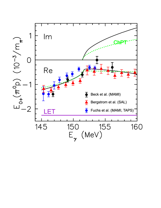
Figure 10: The real (Re) and imaginary (Im) parts of the threshold amplitude $E_{0+}(p\pi^{0})$ as predicted by dispersion relations $\!{}^{{\bf?}}$ (full lines), chiral perturbation theory $\!{}^{{\bf?}}$ (dashed lines), and the “classical” low energy theorem $\!{}^{{\bf?}}$ (LET). Experimental data from MAMI $\!{}^{{\bf?},{\bf?}}$ and SAL $\!{}^{{\bf?}}$.

6.2 Pion production in the resonance region

The search for a deformation of the “elementary” particles is a longstanding issue. Such a deformation is evidence for a strong tensor force between the constituents, originating in the case of the nucleon from the residual force of gluon exchange. Depending on one’s favourite model, such effects can be described by d-state admixture in the quark wave function $\!{}^{{\bf?}}$, tensor correlations between the pion cloud and the quark bag $\!{}^{{\bf?},{\bf?}}$, or by exchange currents accompanying the exchange of mesons between the quarks $\!{}^{{\bf?}}$. Unfortunately, it would require a target with a spin of at least 3/2 (e.g. $\Delta$ matter) to observe a static deformation. An alternative is to measure the transition quadrupole moment between the nucleon and the $\Delta$, i.e. the amplitude $E_{1+}$, which is sensitive to model parameters responsible for a possible deformation of the hadrons.

The experimental quantity of interest is the ratio $R_{EM}=E_{1+}/M_{1+}$ in the region of the $\Delta$. The two amplitudes $E_{1+}$ and $M_{1+}$ are related to the helicity amplitudes, which may be determined by scattering an incident photon with circular polarization off a target nucleon with its spin oriented in the direction or opposite to the photon momentum $\vec{q}$,

$$A_{1} = A_{1/2}=\frac{1}{\sqrt{2q}}\left\langle N^{\ast}(J,M=\frac{1}{2})\mid J_{+}\mid N(J_{i}=\frac{1}{2},M_{i}=-\frac{1}{2})\right\rangle$$

$$A_{3} = A_{3/2}=\frac{1}{\sqrt{2q}}\left\langle N^{\ast}(J,M=\frac{3}{2})\mid J_{+}\mid N(J_{i}=\frac{1}{2},M_{i}=+\frac{1}{2})\right\rangle,$$ (72)

where $J_{+}$ is the hadronic current corresponding to the absorption of a photon with positive helicity on the nucleon $N$ with spin $J_{i}=\frac{1}{2}$ and spin projection $M_{i}$, leading to a resonance state $N^{\ast}$ with spin $J\geq\frac{1}{2}$ and spin projection $M$. It is obvious that all resonances can generally contribute to $A_{1}$, while only resonances with $J\geq\frac{3}{2}$ will contribute to $A_{3}$. The helicity-conserving process $A_{1}$ can also occur on an individual (massless) quark, whereas $A_{3}$ is forbidden in that approximation. Hence perturbative QCD predicts that $A_{3}$ should vanish for high momentum transfer, i.e. for electroproduction and $Q^{2}=\vec{q}^{\ 2}-\omega^{2}\rightarrow\infty$.

We shall now compare the prediction of Kälbermann and Eisenberg  $\!{}^{{\bf?}}$ with our analysis of the modern pion photoproduction data $\!{}^{{\bf?},{\bf?}}$. The helicity amplitudes for the $N\rightarrow\Delta$ transition will be given in the usual units of 10^-3 GeV${}^{-\frac{1}{2}}$, and the prediction of Ref. $\!{}^{{\bf?}}$ is obtained for a bag radius of 1 fm, which was the preferred value in the 1980’s. The result is

$$\begin{array}[]{ll}{\rm{Ref.~{}^{74}:}}\ \ A_{1}=-130&A_{3}=-250\\ {\rm{Ref.~{}^{58}:}}\ A_{1}=-131\pm 1&A_{3}=-252\pm 1\ ,\end{array}$$

the agreement being truly astounding though somewhat accidental, because the theoretical value depends on the bag radius. However, the result is relatively stable, even a drastic decrease of the bag radius to 0.6 fm will change the helicity amplitudes by only 10%. This success of the chiral bag model is even more outstanding when compared with the results of the quark model without pionic degress of freedom. From a selection of ten quark model calculations published over the past 20 years we find $-113\leq A_{1}\leq-82$ and $-195\leq A_{3}\leq-58$, values far off the experimental data.

The helicity amplitudes are related to the electric and magnetic multipoles,

$$M_{1^{+}} = -\frac{1}{2\sqrt{3}}(\sqrt{3}\ A_{1/2}+3\ A_{3/2})\ ,$$

$$E_{1^{+}} = -\frac{1}{2\sqrt{3}}(\sqrt{3}\ A_{1/2}-A_{3/2})\ .$$ (73)

Since $A_{\frac{3}{2}}\simeq\sqrt{3}\ A_{\frac{1}{2}}$ according to Eq. (6.2), the model predicts that $E_{1^{+}}$ (electric quadrupole excitation $E2$) is very much smaller than $M_{1^{+}}$ (magnetic dipole excitation $M1$). A few years after the pioneering work of Ref. $\!{}^{{\bf?}}$, we obtained, for a bag radius of 0.6 fm, the ratio $R=E_{1^{+}}/M_{1^{+}}=-2.8\%$ $\!{}^{{\bf?}}$. This result differed by a factor of two from the then accepted experimental value $R_{1988}\simeq-1.3\%$. However, it is quite close to the recent MAMI data of Beck et al.  $\!{}^{{\bf?}}$, $R_{1997}=(-2.5\pm 0.2\pm 0.2)\%$, and to our global analysis of the data $\!{}^{{\bf?}}$, $R_{1998}=(-2.5\pm 0.1)\%$.

As may be seen from Fig. 11 , the ratio $R=R_{EM}$ changes rapidly with the energy $W_{cm}$ of the pion-nucleon system. The reason for this energy dependence is the nonresonant background, which is particularly large in the case of the small $E_{1^{+}}$ multipole. The historically first prediction of that number is due to Chew et al. $\!{}^{{\bf?}}$ in 1957 who found $R\simeq 0$ from a dispersion theoretical analysis. Such value was later explained by Becchi and Morpurgo $\!{}^{{\bf?}}$ in the framework of the constituent quark model. In the following years the quark models were refined by introducing tensor correlations, with the result of finite, small and usually negative values for $R$. Such correlations have been motivated in different ways, by hyperfine interactions between the quarks $\!{}^{{\bf?}}$, pion-loop effects $\!{}^{{\bf?}}$ and, more recently, exchange currents $\!{}^{{\bf?}}$. In analogy with heavy even-even nuclei having “intrinsic” deformation, finite values of $E2$ are often referred to as ”bag deformation” or ”deformation of the nucleon”, although a quadrupole moment cannot be observed for an object with spin $J<1$. Ideally one could probe the static quadrupole moment of the $\Delta$ by experiments like $\pi N\rightarrow\Delta\rightarrow\Delta\gamma\rightarrow\pi N\gamma$, however a closer look shows that this is hardly a realistic possibility. In conclusion it is precisely the $N\Delta$ transition quadrupole moment that provides us with information on tensor correlations in the nucleon, which can be translated, e.g., into a $d$-state admixture in the quark wave function. In such a model the $\Delta$ would have an oblate deformation, much smaller than a frisbee and much larger than the earth, in absolute numbers quite comparable to the deuteron, which however has a prolate deformation.

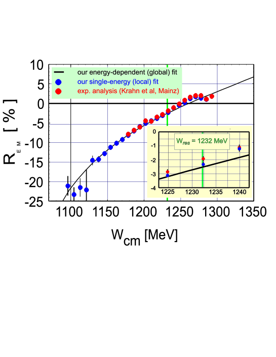
Figure 11: The ratio $R_{EM}=R$ as function of the energy $W_{cm}$ of the pion-nucleon system. See Refs. $\!{}^{{\bf?},{\bf?}}$ and references given therein

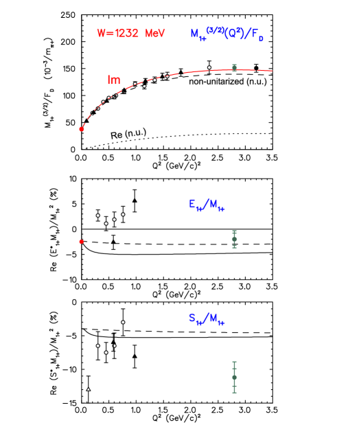
Figure 12: The amplitudes for $\Delta$ excitation as function of $Q^{2}$. Top: $M_{1+}$ divided by the dipole form factor $F_{D}=G_{D}$, center: the ratio $E_{1+}/M_{1+}$, bottom: the ratio $S_{1+}/M_{1+}$. See text and Ref. $\!{}^{{\bf?}}$.

Meson electroproduction allows us to study the dependence of the multipoles on momentum transfer, $M_{l\pm}=M_{l\pm}(Q^{2})$, i.e. to probe the spatial distribution of the transition strength. In addition, the virtual photon carries a longitudinal field introducing a further multipole, $S_{l\pm}$. The $Q^{2}$ dependence of the $N\Delta$ multipoles is displayed in Fig. 12. In the top figure, we show the results for the magnetic multipole divided by the standard dipole form factor. The data are compared to the predictions of our unitary isobar model (UIM) $\!{}^{{\bf?}}$. This model contains the usual Born terms, vector meson exchange in the t-channel and nucleon resonances in the s-channel, unitarized partial wave by partial wave with the appropriate pion-nucleon phases and inelasticities. The center piece of Fig. 12 shows the ratio $R=R(Q^{2})$ compared to mostly older and strongly fluctuating data. More recent data from Jefferson Lab $\!{}^{{\bf?}}$ indicate, however, that even at $Q^{2}\approx 2.8$ and 4 (GeV/c)² this ratio remains negative and of the order of a few per cent. This is surprising, because perturbative QCD predicts that the helicity amplitude $A_{3}$ should vanish for $Q^{2}\rightarrow\infty$ and, hence, the ratio $R$ should approach +100% (see Eq. (73)). Finally, the bottom figure shows the corresponding longitudinal-transverse ratio $S_{1^{+}}/M_{1^{+}}$. Recent experimental data at ELSA, MAMI and MIT $\!{}^{{\bf?}}$ at $Q^{2}\approx 0.5$ (GeV/c$)^{2}$ yield ratios of about -7 %, slightly below our prediction, while the preliminary data from the Jefferson Lab $\!{}^{{\bf?}}$ at larger $Q^{2}$ seem to indicate considerably lower values between -10 % and -20 %. From perturbative QCD one expects that this ratio should vanish for $Q^{2}\rightarrow\infty$.

The modern precision experiments will be continued to the higher resonances. Concerning the $N^{\ast}$(1440) or Roper resonance, both data and predictions are still in a deploratory state, and it will require double-polarization experiments to find out about the nature of that resonance. One possibility to tackle the problem will be pion production by linearly polarized photons on longitudinally polarized protons. Such an experiment measures the polarization observable $G\sim ImM_{1^{-}}ReM_{1^{+}}$, i.e. an interference of the $\Delta$ resonance with the absorptive part of the Roper multipole $M_{1^{-}}$.

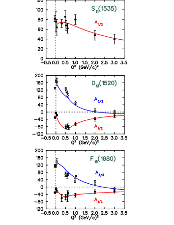
Figure 13: The helicity amplitudes $A_{1/2}^{p}$ and $A_{3/2}^{p}$ for the resonances $S_{11}$(1535), $D_{13}(1520)$, and $F_{15}(1680)$ as functions of $Q^{2}$. See text and Ref. $\!{}^{{\bf?}}$.

The existing information on some of the higher resonances is shown in Fig. 13. For our discussion in the next chapter it is important to note:

1. Because of its quantum numbers $J^{P}=\frac{1}{2}^{-}$, the resonance $S_{11}$(1535) is only excited via the $A_{1/2}$ amplitude. As function of $Q^{2}$, this amplitude drops much slower than any other resonance of the nucleon. With a resonance position very close to $\eta$ production threshold, the $S_{11}$(1535) has an $\eta$ branching ratio of about 50 %, while this ratio is of the order of 1 % or less for all other resonances.

2. The resonances $D_{13}$(1520) and $F_{15}$(1680) carry most of the electric dipole and quadrupole strengths, respectively. For real photons $(Q^{2}=0)$ their helicity amplitudes $A_{1/2}^{p}$ are nearly zero, but already at $Q^{2}\approx 0.5$ (GeV/c)² $A_{1/2}^{p}$ and $A_{3/2}^{p}$ are of equal importance, and in accordance with pQCD, $A_{3/2}^{p}$ decreases rapidly for $Q^{2}\rightarrow\infty$.

7 SUM RULES

As has been stated in Eq. (57), the GDH sum rule connects the integral

$$I=\int_{\nu_{0}}^{\infty}\frac{\sigma_{1/2}(\nu)-\sigma_{3/2}(\nu)}{\nu}d\nu$$ (74)

with the anomalous magnetic moment.

On the basis of the pion-nucleon multipoles and certain assumptions for the higher channels, various authors have estimated this integral. As shown in Table 4, the absolute value of the proton integral $I_{p}$ has been consistently overpredicted, while the neutron integral $I_{n}$ comes out too small. This has the consequence that not even the sign of the isovector combination $I_{p}-I_{n}$ agrees with the sum rule value. This apparent discrepancy has led to speculations that the GDH integral should not converge for various reasons, e.g. due to a generalized current algebra, because of fixed axial vector poles or influences of the Higgs particle. None of these arguments is too convincing at present. In fact one should realize that the GDH integrand is an oscillating function of photon energy, with multipole contributions of alternating sign. Therefore, little details matter and a stable result requires very exact data. Comparing again the results obtained with the SAID $\!{}^{{\bf?}}$ and HDT $\!{}^{{\bf?}}$ multipoles, the generally accepted threshold value of $E_{0^{+}}$ reduces the “discrepancy” with the sum rule value by about $25\%$ (see Table 4 and Ref. $\!{}^{{\bf?}}$).

Table 4: Predictions for the GDH integral for proton $(I^{p}$), neutron $(I^{n}$), and the difference $I^{p}-I^{n}$ in units of $\mu$b. With the exception of Ref. $\!{}^{{\bf?}}$, the two-pion contribution has been taken from Ref. $\!{}^{{\bf?}}$.

	$I^{p}$	$I^{n}$	$I^{p}-I^{n}$
GDH	-205	-233	28
Ref. $\!{}^{{\bf?}}$	-261	-183	-78
Ref. $\!{}^{{\bf?}}$	-260	-157	-103
Ref. $\!{}^{{\bf?}}$	- 223
Ref. $\!{}^{{\bf?}}$	- 289	-160	- 129
Ref. $\!{}^{{\bf?}}$	-261	-180	-81

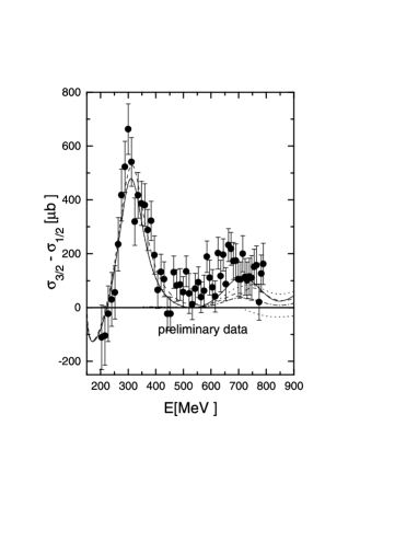
Figure 14: The difference of the helicity cross section, $\sigma_{3/2}-\sigma_{1/2}$, as function of the $lab$ energy $\nu=E$ of the photon. The theoretical predictions of Refs. $\!{}^{{\bf?},{\bf?}}$ are compared to the preliminary data of the 1998 MAMI experiment⁵⁷.

The first direct measurement of the helicity cross sections was recently performed at MAMI in the energy region 200 MeV $<\nu<800$ MeV $\!{}^{{\bf?}}$. The experiment will be extended to the higher energies at ELSA. Some preliminary results are shown in Fig. 14, which contains only 5 % of the data taken in the 1998 run. The figure shows the importance of charged pion production near threshold (multipole $E_{0+}$), and the dominance of the multipole $M_{1+}^{3/2}$ in the $\Delta$ resonance region. At yet higher energies the data lie above the prediction for one-pion production, which indicates considerable two-pion contributions. These data establish that the forward spin polarizability should be $\gamma_{0}\approx-0.8\cdot 10^{-4}$ fm⁴. Furthermore the preliminary data saturate the GDH sum rule at $\nu\approx 800$ MeV if one accepts our predictions $\!{}^{{\bf?}}$ for the energy range between threshold and 200 MeV. However, more data are urgently required at energies both below 200 MeV and above 800 MeV.

In view of the difficulty to obtain even the proper sign for the proton-neutron difference from the older data (see Table 4), it is of considerable interest to measure the GDH for the neutron. However, such investigations are difficult due to nuclear binding effects. While it is generally assumed that ²H and ³He are good neutron targets, the sum rule requires to integrate over all regions of phase space and not only the region of quasifree kinematics. In fact there exists a GDH sum rule for systems of any spin, and hence every nucleus should have a well-defined value for the GDH integral. With the definition of Table 4, one finds the small value $I(^{2}$H$)=-0.65~{}\mu$b due to the fact that the deutron lies very close to the Schmidt line. However, a loosely bound system of neutron and proton would be expected to have $I_{p}+I_{n}=-438~{}\mu$b, which differs by 3 orders of magnitude from the deuteron value! Obviously the large contributions from pion production have to be canceled by binding effects in the deuteron. As has been shown by Arenhövel and collaborators $\!{}^{{\bf?}}$, such contribution is mainly due to the transition from the ³S₁ ground state of ²H to the ¹S₀ resonance at 68 keV. Weighted with the inverse power of excitation energy, the absorption cross section for this low-lying resonance cancels the huge cross sections due to pion production. We note that the opposite sign of the two contributions is due to the fact that the spins of the 3 quarks become aligned by the transition $N\rightarrow\Delta$, while the nucleon spins are parallel in the deuteron $(^{3}$S₁) but antiparallel in the ¹S resonance. However, in addition to this low lying resonance, there are also sizeable sum rule contributions by break-up reactions $\gamma+d\rightarrow n+p$ in the range below and above pion threshold. Such effects are usually triggered by meson exchange currents (the virtual pions below or the real pions above threshold are reabsorbed by the other nucleon) or isobaric currents (a $\Delta$ is produced but decays by final state interaction without emitting a pion). In addition there are also contributions of coherent $\pi^{0}$ production, i.e. $\gamma+d\rightarrow\pi^{0}+d$. It is general to all these processes that they cannot occur on a free nucleon, though they are certainly driven by pion production and nucleon resonances. This leads to the serious question: Which part of the GDH integral is nuclear structure and hence should be subtracted, and how should one divide the rest into the contributions of protons and neutrons? The problem is not restricted to the deuteron but quite general. For example the “neutron target” ³He has the same sum rule as the nucleon except that one has to replace $e,\ m$ and $\kappa$ of the nucleon by the charge $(Q=2e)$, mass $(M\approx 3m_{N})$ and anomalous magnetic moment of ³He. The result is $I(^{3}$He$)=-496~{}\mu$b, while we naively expect $I_{n}=-233~{}\mu$b, because the spins of the two protons are antiparallel and hence should not contribute to the helicity asymmetry.

These considerations can be generalized to virtual photons by electron scattering. While the coincidence cross section for the reaction $\vec{e}+\vec{p}\rightarrow e^{\prime}+N+\pi$ contains 18 different response functions $\!{}^{{\bf?}}$, only 4 responses remain after integration over the angles of pion emission, which is exactly the result of Eq. (17). The 4 partial cross sections can in principle be separated by a super-Rosenbluth plot if one varies the polarizations. These are the transverse polarizations $\varepsilon$ of the virtual photon, the polarization $P_{e}$ of the electron ($\pm 1$ for the relativistic case), and the nucleon’s polarization in the scattering plane of the electron, with components $P_{z}$ in the direction and $P_{x}$ perpendicular to the virtual photon momentum.

The multipole content of one-pion production to the partial cross sections is $\!{}^{{\bf?},{\bf?}}$

$$\sigma_{T}^{(1\pi)} = 4\pi\frac{|{\bf k}_{\pi}^{cm}|}{k^{cm}}\sum_{l}\frac{1}{2}(l+1)^{2}$$

$$\cdot[(l+2)(|E_{l+}|^{2}+|M_{l+1,-}|^{2})+l(|M_{l+}|^{2}+|E_{l+1,-}|^{2})]$$

$$= 4\pi\frac{|{\bf k}_{\pi}^{cm}|}{k^{cm}}\{|E_{0+}|^{2}+2|M_{1+}|^{2}+6|E_{1+}|^{2}+|M_{1-}|^{2}+2|E_{2-}|^{2}\pm\ ...\}\ ,$$

$$\sigma_{L}^{(1\pi)} = 4\pi\frac{|{\bf k}_{\pi}^{cm}|}{k^{cm}}\left(\frac{Q}{\omega^{cm}}\right)^{2}\sum_{l}\frac{1}{2}(l+1)^{3}[|L_{1+}|^{2}+|L_{l+1,-}|^{2}]$$

$$= 4\pi\frac{|{\bf k}_{\pi}^{cm}|}{k^{cm}}\left(\frac{Q}{\omega^{cm}}\right)^{2}\left\{|L_{0+}|^{2}+8|L_{1+}|^{2}+|L_{1-}|^{2}+8|L_{2-}|^{2}\pm\ ...\right\}\ ,$$

$$\sigma_{TT^{\prime}}^{(1\pi)} = 4\pi\frac{|{\bf k}_{\pi}^{cm}|}{k^{cm}}\sum_{l}\frac{1}{2}(l+1)[-(l+2)(|E_{l+}|^{2}+|M_{l+1,-}|^{2})$$

$$+l(|M_{l+}|^{2}+|E_{l+1,-}|^{2})-2l(l+2)(E_{l+}^{\ast}M_{l+}-E^{\ast}_{l+1,-}M_{l+1,-})]$$

$$= 4\pi\frac{|{\bf k}_{\pi}^{cm}|}{k^{cm}}\{-|E_{0+}|^{2}+|M_{1+}|^{2}-6E_{1+}^{\ast}M_{1+}-3|E_{1+}|^{2}+|E_{2-}|^{2}\pm\ ...\}\,$$

$$\sigma_{LT^{\prime}}^{(1\pi)} = 4\pi\frac{|{\bf k}_{\pi}^{cm}|}{k^{cm}}\left(\frac{Q}{\omega^{cm}}\right)\sum_{l}\frac{1}{2}(l+1)^{2}$$

$$\cdot[-L_{l+}^{\ast}((l+2)E_{l+}+lM_{l+})+L_{l+1,-}^{\ast}(lE_{1+,-}+(l+2)M_{l+1,-})]$$

$$= 4\pi\frac{|{\bf k}_{\pi}^{cm}|}{k^{cm}}\left(\frac{Q}{\omega^{cm}}\right)\{-L_{0+}^{\ast}E_{0+}-2L_{l+}^{\ast}(M_{1+}+3E_{1+})$$

$$+L_{1-}^{\ast}M_{1-}+L_{2-}^{\ast}E_{2-}\pm\ ...\}\ .$$

Since the partial wave decomposition is defined in the hadronic $cm$ frame, the appropriate $cm$ values of the kinematical observables have to be used in these equations, in particular the $cm$ momentum and the $cm$ energy of the virtual photon, $k^{cm}=\frac{m}{W}k$ and $\omega^{cm}=\frac{1}{W}\sqrt{m^{2}\nu^{2}-Q^{2}(W^{2}-m^{2})}$ respectively. We note that $\omega^{cm}$ has a zero if $W=\sqrt{m^{2}+Q^{2}}$, which is compensated by a corresponding zero in the longitudinal multipole. This situation can be avoided by using the “scalar” multipoles (rather to be called “Coulomb” or “time-like” multipoles!),

$$S_{l\pm}=\frac{k^{cm}}{\omega^{cm}}L_{l\pm}\ .$$ (79)

While $\sigma_{T}$ and $\sigma_{L}$ are the sum of squares of transverse $(E_{l\pm},M_{l\pm})$ and longitudinal $(L_{l\pm})$ multipoles respectively, the interference structure functions $\sigma^{\prime}_{TT}=(\sigma_{3/2}-\sigma_{1/2})/2$ and $\sigma^{\prime}_{LT}$ contain multipole contributions of alternating sign. The multipoles involved are now functions of energy and momentum transfer, ${\cal M}_{l\pm}={\cal M}_{l\pm}(\nu,Q^{2})$.

The 4 cross sections are related to the familiar structure functions of deep inelastic lepton scattering,

$$\{\sigma_{T}\ ,\sigma_{L}\ ;\ \sigma^{\prime}_{LT}\ ,\sigma^{\prime}_{TT}\}\Longrightarrow\{F_{1}\ ,F_{2}\ ;G_{1}\ ,G_{2}\}\ .$$ (80)

In the Bjorken scaling region, the 2 arguments $\nu$ and $Q^{2}$ of these functions can be replaced by the scaling variable $x=Q^{2}/2m\nu$, which leads to the definition of quark distribution functions. For the spin structure functions $G_{1}$ and $G_{2}$ we find

$$g_{1}(\nu,Q^{2}) = \frac{\nu}{m}\ G_{1}(\nu,Q^{2})\rightarrow\ g_{1}(x)=\frac{1}{2}\sum e^{2}_{i}(f_{i}^{\uparrow}-f_{i}^{\downarrow})$$

$$g_{2}(\nu,Q^{2}) = \frac{\nu^{2}}{m^{2}}\ G_{2}(\nu,Q^{2})\rightarrow g_{2}(x)=\frac{1}{2}\sum e^{2}_{i}(f_{i}^{\rightarrow}-f_{i}^{\leftarrow})\ ,$$ (81)

where the arrows indicate the different directions of the quark spins. With these definitions we can express a set of generalized sum rules in terms of both the quark spin functions of Eq. (7) and the cross sections of Eq. (79), e.g.

$$I_{1}(Q^{2}) = \int_{\nu_{0}}^{\infty}\frac{d\nu}{\nu}\ G_{1}(\nu,Q^{2})=\frac{2m}{Q^{2}}\int_{0}^{x_{0}}dx\ g_{1}(x,Q^{2})\rightarrow\frac{2m^{2}}{Q^{2}}\Gamma$$ (82)

$$= \frac{m^{2}}{2\pi e^{2}}\int^{\infty}_{\nu_{0}}d\nu\ (1-x)\ \left(\sigma_{1/2}-\sigma_{3/2}+2\frac{Q}{\nu}\sigma^{\prime}_{LT}\right)\ ,$$

$$I_{2}(Q^{2}) = \frac{1}{m}\int^{\infty}_{\nu_{0}}d\nu\ G_{2}(\nu,Q^{2})=\frac{2m^{2}}{Q^{2}}\int^{x_{0}}_{0}dx\ g_{2}(x,Q^{2})$$ (83)

$$= \frac{m^{2}}{2\pi e^{2}}\int^{\infty}_{\nu_{0}}d\nu\ (1-x)\ \left(-\sigma_{1/2}+\sigma_{3/2}+2\frac{\nu}{Q}\sigma^{\prime}_{LT}\right)\ ,$$

with $\nu_{0}$ and $x_{0}$ the lowest threshold for inelastic reactions.

Eq. (82) is a possible generalization of the GDH sum rule, because $I_{1}(0)=-\kappa^{2}/4$. However, a large variety of generalized GDH sum rules can be obtained by adding different fractions of the interference term $\frac{Q}{\nu}\sigma^{\prime}_{LT}$, which vanishes both in the real photon limit, $Q^{2}\rightarrow 0$, and in the asymptotic region, $Q^{2}\rightarrow\infty$. The most obvious choice would be to simply drop this term in Eq. (82). As it stands, however, the definition of $I_{1}$ is the natural definition of an integral over the spin structure function $g_{1}$. In particular it has the asymptotic behaviour indicated in Eq. (82), with $\Gamma$ a constant. The fact that the experimental value of $\Gamma$ differed from earlier predictions $\!{}^{{\bf?}}$ led to the “spin crisis” and taught us that less than half of the nucleon’s spin is carried by the quarks $\!{}^{{\bf?}}$.

The integral Eq. (83) for the second spin structure functions $G_{2}$ shows distinct differences in comparison with Eq. (82). First, the helicity cross sections $\sigma_{1/2}$ and $\sigma_{3/2}$ appear with different sign. This has the consequence that in the sum $I_{1+2}=I_{1}+I_{2}$ only the longitudinal-transverse contribution $\sigma^{\prime}_{LT}$ remains. Second, the latter contribution now appears as $\frac{\nu}{Q}\sigma^{\prime}_{LT}$, which is finite in the real-photon limit, $Q^{2}\rightarrow 0$. While the generalized GDH integral of Eq. (82) ist not a sum rule, i.e. not related to another observable except for the real photon point, the Burkhardt-Cottingham (BC) sum rule predicts that $I_{2}(Q^{2})$ can be expressed by the magnetic $(G_{M})$ and electric $(G_{E})$ Sachs form factors at each momentum transfer $\!{}^{{\bf?}}$,

$$I_{2}(Q^{2})=\frac{1}{4}G_{M}(Q^{2})\frac{G_{M}(Q^{2})-G_{E}(Q^{2})}{1+Q^{2}/4m^{2}}\ .$$ (84)

According to Eq. (84) the integral $I_{2}$ approaches the value $\kappa\mu/4$ for real photons $(Q^{2}=0)$ and drops with $Q^{-10}$ for $Q^{2}\rightarrow\infty$. As a result the sum $I_{1+2}(0)$ should take the value $\kappa(\mu-1)/4$, i.e. $\kappa^{2}/4$ and 0 for proton and neutron respectively. However, there are strong indications that the BC integrand gets large contributions at higher energies, which in fact will affect its convergence. At least for the proton, however, the “sum rule” seems to work quite well if we restrict ourselves to the resonance region.

In the case of the proton, the GDH sum rule predicts $\Gamma_{1}<0$ for small $Q^{2}$, while all experiments for $Q^{2}>1$ (GeV/c)² yield positive values. Clearly, the value of the sum rule has to change rapidly at low $Q^{2}$, with some zero-crossing at $Q^{2}_{0}<1$ (GeV/c)². This evolution of the sum rule was first parametrized by Anselmino et al. $\!{}^{{\bf?}}$ in terms of vector meson dominance. Burkert, Ioffe and others $\!{}^{{\bf?}}$ refined this model considerably by treating the contributions of the resonances explicitly. Soffer and Teryaev $\!{}^{{\bf?}}$ suggested that the rapid fluctuation of $I_{1}$ should be analyzed in conjunction with $I_{2}$, because $I_{1}+I_{2}$ is known for both $Q^{2}=0$ and $Q^{2}\rightarrow\infty$. Though this sum is related to the practically unknown longitudinal-transverse interference cross section $\sigma^{\prime}_{LT}$ and therefore not yet determined directly, it can be extrapolated smoothly between the two limiting values of $Q^{2}$. The rapid fluctuation of $I_{1}$ then follows by subtraction of the BC value of $I_{2}$. We also refer the reader to a recent evaluation of the $Q^{2}$-dependence of the GDH sum rule in a constituent quark model $\!{}^{{\bf?}}$, and to a discussion of the constraints provided by chiral perturbation theory at low $Q^{2}$ and twist-expansions at high $Q^{2}$ (see Ref. $\!{}^{{\bf?}}$).

Figure 15: The integrals $I_{1}$ and $I_{2}$ defined by Eqs. (82) and (83) as functions of $Q^{2}$ in the resonance region, integrated up to $W_{max}=2$ GeV. Upper figure: Dashed, dotted and solid curves are calculations obtained with $1\pi,1\pi+\eta$, and $1\pi+\eta+n\pi$ contributions, and data from Ref. $\!{}^{{\bf?}}$. Lower figure: The full and dashed lines are our predictions $\!{}^{{\bf?}}$ with and without $\sigma^{\prime}_{LT}$ [see Eq. (83)], the dash-dotted line is obtained for the estimate $\sigma^{\prime}_{LT}=\sqrt{\sigma_{L}\sigma_{T}}$, and the dotted line is the sum rule prediction of Ref. $\!{}^{{\bf?}}$. All calculations for $I_{2}$ include $1\pi+\eta+n\pi$ contributions.

In Fig. 15 we give our predictions $\!{}^{{\bf?}}$ for the integrals $I_{1}(Q^{2})$ and $I_{2}(Q^{2})$ in the resonance region, i.e. integrated up to $W_{max}=2\,GeV$. As can be seen, our model is able to generate the dramatic change in the helicity structure quite well. While this effect is basically due to the single-pion component predicted by the UIM, the eta and multipion channels are quite essential to shift the zero-crossing of $I_{1}$ from $Q^{2}=0.75\,(GeV/c)^{2}$ to 0.52 $(GeV/c)^{2}$ and 0.45 $(GeV/c)^{2}$, respectively. This improves the agreement with the SLAC data $\!{}^{{\bf?}}$. However, some differences remain. Due to a lack of data in the $\Delta$ region, the SLAC data are likely to underestimate the $\Delta$ contribution and thus to overestimate the $I_{1}$ integral or the corresponding first moment $\Gamma_{1}$. A few more data points in the $\Delta$ region would be very useful in order to clarify the situation, and we are looking forward to the results of the current experiments at Jefferson Lab $\!{}^{{\bf?}}$.

Concerning the integral $I_{2}$, our results are in good agreement with the predictions of the BC sum rule (see Fig. 15, lower part). The remaining differences are of the order of $10~{}\%$ and should be attributed to contributions beyond $W_{\rm max}=2$ GeV and the scarce experimental data for $\sigma^{\prime}_{LT}$.

We recall at this point that the results mentioned above refer to the proton. Unfortunately, we find some serious problems for the neutron, for which our model predicts both $I_{1}(0)$ and $I_{2}(0)$ larger than expected from the sum rules. This has the consequence that our prediction for $I_{1+2}(0)$ has a relatively large positive value while it should vanish by sum rule arguments. The reason for this striking discrepancy could well be due to the discussed problems with “neutron targets”. On the other hand it could also be an indication of sizeable contributions at the higher energies, which could possibly cancel for the proton but add in the case of the neutron. In this context it is interesting to note that a recent parametrization of deep inelastic scattering predicts sizeable high-energy contributions with different signs for proton and neutron $\!{}^{{\bf?}}$.

A more general argument is that the convergence of sum rules cannot be given for granted, and thus the good agreement of our model with the BC sum rule could be accidental and due to a particular model prediction for the essentially unknown longitudinal-transverse interference term. As can be seen from Fig. 15, the contribution of $\sigma_{LT^{\prime}}$ is quite substantial for $I_{2}$ even at the real photon point due to the factor $\nu/Q$ in Eq. (83). This contribution, however, is constrained by the positivity relation $|\sigma^{\prime}_{LT}|\leq\sqrt{\sigma_{L}\sigma_{T}}$. The dash-dotted line shows the integral for the upper limit of this inequality and a similar effect would occur for the lower limit. The surprisingly large upper limit can be understood in terms of multipoles. In a realistic description of the integrated cross section $\sigma_{LT^{\prime}}$, the large $M_{1+}$ multipole can only interfer with the small $L_{1+}$ multipole. The upper and lower limits of the positivity relation overestimate the structure function considerably due to an unphysical “interference” between $s$ and $p$ waves.

8 SUMMARY

The new generation of electron accelerators with high energy, intensity and duty-factor has made it possible to perform new classes of coincidence experiments involving polarization observables. These investigations have already provided new data with unprecedented precision, and they will continue to do so for the years to come. Some of the interesting topics and challenging questions are

• a full separation of the electric and magnetic form factors of neutron and proton by double-polarization experiments,

• the search for strange quarks in the nucleon by parity-violating electron scattering,

• new and more precise information on the scalar and vector polarizabilities of the nucleon by a combined analysis of Compton scattering and photoproduction as well as extensions to generalized polarizabilities via virtual Compton scattering,

• the threshold amplitudes for the production of Goldstone bosons and tests of chiral field theories,

• the quadrupole strength for $\Delta_{1232}$ excitation as a measure of tensor correlations among the constituents,

• photo- and electroexcitation of the higher resonances, e.g. the $N^{\ast}_{1440}$ (Why does the Roper occur at such a low excitation energy? Where is its Coulomb monopole strength?), the $N^{\ast}_{1535}$ (Is it really a resonance or a threshold effect of $\eta$ production?), and the helicity structure of the main dipole $(N^{\ast}_{1520})$ and quadrupole ($N^{\ast}_{1680})$ resonances for both proton and neutron,

• investigations of individual decay channels including energy and angular distributions in order to find out how much of the excitation strength is actually due to resonances as opposed to background and threshold effects, and more generally the question how to extract the “intrinsic” quark structure from the experimental data, which necessarily contain the hadronization in terms of mesons,

• ongoing experiments to determine the helicity structure of photo- and electroproduction in the resonance region by use of double-polarization observables, which in turn are related to deep inelastic scattering and the quark spin structure by means of sum rules and related integrals over the excitation spectrum.

Our present understanding of nonperturbative QCD is still in a somewhat deplorable phenomenological state. The ongoing experimental activities will change that situation within short by providing new and detailed information on low-energy QCD in general and the nucleon’s structure in particular. This rich phenomenology will without doubt challenge the theoretical approaches and, as is strongly to be hoped, eventually pave the way for a more quantitative understanding of nonperturbative QCD.

References

TESTS AND PROBLEMS

1. KINEMATICS

2. Prove that $s+t+u=m_{1}^{2}+m_{2}^{2}+m_{3}^{2}+m_{4}^{2}$, for the reaction $p_{1}+p_{2}\rightarrow p_{3}+p_{4}$.

3. Calculate the threshold energy in the lab frame for the reactions

   • $p(\gamma,\gamma^{\prime})p^{\prime}$

   • $p(\gamma,\pi)p^{\prime}$

   • replace the incident real photon by a virtual one with
     $m_{\gamma^{\ast}}^{2}=-Q^{2}<0$

4. Which energy should an accelerator have to electroproduce a $K^{+}$ at $Q^{2}=1$ (GeV/c)²? How much energy would you like to have before you schedule such an experiment?

5. In case of the reaction $p_{1}+p_{2}\rightarrow p_{3}+p_{4}$ with 4 scalar particles, how many Lorentz scalars and vectors can be constructed? How many are independent?

6. Find the kinematical limits for Compton scattering in the s-channel. Use $\nu=(s-u)/4M$ and $t$ as orthogonal coordinates, and relate them in the $cm$ frame for forward and backward scattering. What about the other parts of the hyperbola of Fig. 3?

7. FORM FACTORS

8. Evaluate the vector current $J_{u}=\bar{u}_{p^{\prime}}(F_{1}\gamma_{\mu}+\frac{i\sigma_{\mu\nu}q^{\nu}}{2m}F_{2})u_{p}$ in the Breit frame, $\vec{p}=-\frac{1}{2}\vec{q}$ and $\vec{p}\ ^{\prime}=+\frac{1}{2}\vec{q}$, and identify the Sachs form factors $G_{E}$ and $G_{M}$ of Eq. (23).

9. The electric Sachs form factor of the proton can be approximated by the dipole form $G_{E}^{p}=(1+(Q/.84$ GeV)${}^{2})^{-2}=G_{D}(Q^{2})$. Calculate the charge distribution by a Fourier transform according to Eq. (25).

10. STRANGENESS

11. Derive the structure of the Lorentz tensor $W_{\mu\nu}=J_{\mu}J_{\nu}^{\ast}$, constructed from a general vector current $J_{\mu}$ for an unpolarized fermion. Use independent 4-momenta $q_{\mu}=p_{2\mu}-p_{1\mu}$ and $P_{\mu}=\frac{1}{2}(p_{1\mu}+p_{2\mu})$, and impose current conservation.

12. In the case of $\vec{e}+p\rightarrow e^{\prime}+p^{\prime}$, there also appears an antisymmetric tensor $\eta_{\mu\nu}^{({\cal{A}})}=\frac{i}{2m^{2}}\epsilon_{\mu\nu\alpha\beta}q^{\alpha}P^{\beta}$ with a $\pm$ sign in front depending on the helicity of the electron. Why does this term not contribute to the cross section derived from photon exchange? What would be required to see this term?

13. A simple model of the proton says that part of the time it appears as a neutron surrounded by a $\pi^{+}$ cloud. If this system has orbital momentum $l=l_{z}=1$, with which probability should it occur in order to describe the anomalous magnetic moment $\kappa_{p}$ of the proton?

14. Estimate the contribution of $\Lambda^{\circ}K^{+}$ configurations to the strangeness form factors of Eq. (32) following the procedure of No 10. Which sign does the strangeness magnetic moment $\mu^{s}$ carry according to the model? What about the strangeness radius $<r^{2}>_{s}$?

15. COMPTON SCATTERING

16. Derive an upper limit for the electric polarizability of proton and neutron in a two-body model as in No 10. Use the definition of Eq. (45) and note that the excitation spectrum lies at $E_{n}-E_{0}>m_{\pi}$. Express the result in terms of the radius $<r^{2}>_{E}^{n,p}$. How general is the result?

17. A generic model of a polarizable system is the following (see Ref. $\!{}^{{\bf?}}$): Two objects with masses $M_{1,2}$ and charges $Q_{1,2}$ are bound by a spring (oscillator frequency $\omega_{0}^{2}=C/\mu$, $C=$ Hooke’s constant, $\mu=$ reduced mass). An electric $\vec{E}=\vec{E}_{0}e^{i\omega t}$ induces a dipole moment $\vec{D}=\alpha(\omega)\vec{E}_{0}$.

    • Determine $\alpha(\omega)$ and consider the cases of (I) equal particles, (II) $M_{2}\rightarrow\infty$, $Q_{2}\rightarrow 0$.

    • If $Q=Q_{1}+Q_{2}\neq 0$, the system will be accelerated even in the limit $\omega\rightarrow 0$. Calculate $\vec{D}^{\bullet\bullet}$ for the $cm$ coordinate.

    • Calculate $\vec{D}^{\bullet\bullet}$ for the relative coordinate.

    • Classical antenna theory says that the cross section is

      $$\frac{d\sigma}{d\Omega}=|f(\omega)|^{2}\sim\left(\frac{|\vec{D}^{\bullet\bullet}|}{|\vec{E}|}\right)^{2}\ .$$

      Compare this result with Eq. (48) and discuss the scattering amplitude $f$ and the cross section for $\omega=0$, $\omega\ll\omega_{0}$, $\omega\approx\omega_{0}$ and $\omega\gg\omega_{0}$. Which kind of scattering occurs for $Q=0$?

18. Estimate the polarizability for the following systems, approximated by 2-body configurations, using the result of No 13 (see Ref. $\!{}^{{\bf?}}$).

    • H atom = $p+e^{-}$ ,     $\hbar\omega_{0}\sim 10$ eV

    • deuteron = $p+n$ ,    $\hbar\omega_{0}\sim 4.5$ eV

    • ${}^{208}Pb=82p+126n$ , $\hbar\omega_{0}\sim 14$ eV

    • $p=2u+1d$ ,            $\hbar\omega_{0}\sim 500$ eV

    • $n=1u+2d$ ,           $\hbar\omega_{0}\sim 500$ eV

19. PION PHOTOPRODUCTION

20. Threshold pion production is given by the s-wave multipoles $E_{0+}$. Estimate these multipoles for the 4 physical channels $\gamma+{\cal{N}}\rightarrow\pi+{\cal{N}}$ by evaluating the squares of the electric dipole moments of the $\pi{\cal{N}}$ configuration. Compare these results with Table 3.

21. Which multipoles connect the ${\cal{N}}$ with the following resonances:
    $P_{33}(1232),\ J^{p}=\frac{3}{2}^{+}$; $P_{11}(1440),\ J^{p}=\frac{1}{2}^{+};\\ D_{13}(1520),\ J^{p}=\frac{3}{2}^{-};\ S_{11}(1535)$, $J^{p}=\frac{1}{2}^{-};\\ F_{15}(1680),\ J^{p}=\frac{5}{2}^{+}$.
    See Eq. (67) and the text following that equation.

22. SUM RULES

23. The integrand of the GDH sum rule has the multipole decomposition of Eq. (76). Draw a figure of the GDH integrand for the 4 physical channels as function of $\omega$, using the result of No. 16 and the information given in Section 6.

24. A possible generalization $I_{GDH}$ of the GDH integral is obtained from Eq. (83) by dropping the term in $\sigma_{LT}^{\prime}$. Discuss the sign of $I_{GDH}$ for $Q^{2}\Rightarrow 0$ and $Q^{2}\Rightarrow\infty$. Give qualitative arguments why the sign change takes place already at relatively small $Q^{2}$.

References

-
[1]
For a general introduction to QCD see
E. S. Abers and B. W. Lee, Phys. Rep. 9 (1973) 1; W. Marciano and H. Pagels, Phys. Rep. 36 (1978) 137; G. Altarelli, Phys. Rep. 81 (1982) 1; H. Georgi, Weak Interactions and Modern Particle Theory, Benjamin/Cummings (1984). - [2] J. Gasser and H. Leutwyler, Ann. Phys. (N.Y.) 158 (1984) 142, and Nucl. Phys. B 250 (1985) 465.
- [3] V. Bernard et al., Int. J. Mod. Phys. E 4 (1995) 193.
- [4] D. Drechsel, Prog. Part. Nucl. Phys. 34 (1995) 181.
- [5] D. Drechsel and L. Tiator, J. Phys. G: Nucl. Part. Phys. 18 (1992) 449.
- [6] R. G. Sachs, Phys. Rev. 126 (1962) 2256.
- [7] N. Isgur, Phys. Rev. Lett. 83 (1999) 272.
- [8] P. Bosted et al., Phys. Rev. Lett. 68 (1992) 3841; A. F. Sill et al., Phys. Rev. D 48 (1993) 29.
- [9] R. G. Arnold et al., Phys. Rev C 23 (1981) 363.
- [10] H.-W. Hammer, U.-G. Meißner, and D. Drechsel, Phys. Lett. B 385 (1996) 343.
- [11] R. G. Arnold et al., Phys. Rev. Lett. 57 (1986) 174.
- [12] M. K. Jones et al., nucl-ex/9910005.
- [13] S. Kopecky et al., Phys. Rev. C 56 (1997) 2229.
- [14] W. Bartel et al., Nucl. Phys. B 58 (1973) 429.
- [15] S. Platchkov et al., Nucl. Phys. A 510 (1990) 740.
- [16] M. Ostrick et al., Phys. Rev. Lett. 83 (1999) 276; C. Herberg et al., Eur. Phys. Journ. A 5 (1999) 131; D. Rohe et al., Phys. Rev. Lett. 83 (1999) 4257; J. Becker et al., Eur. Phys. Journ. A 6 (1999) 329, and references given therein.
- [17] H. Arenhövel, Phys. Lett. B 199 (1987) 13; Z. Phys. A 331 (1988) 509; and private communication.
- [18] D. H. Lu, A. W. Thomas, and A. G. Williams, Phys. Rev. C 57 (1998) 2628.
- [19] H. Schmieden, private communication.
- [20] L. Hand, D. I. Miller, and R. Wilson, Rev. Mod. Phys. 35 (1963) 335.
- [21] G. G. Simon, Ch. Schmitt, F. Borkowski, and V. H. Walther, Nucl. Phys. A 333 (1980) 381.
- [22] S. G. Karshenboim, Phys. Lett. A 225 (1997) 97 and references given therein.
- [23] R. Rosenfelder, nucl-th/9912031.
- [24] J. Ellis and R. L. Jaffe, Phys. Rev. D 9 (1974) 1444 and D 10 (1974) 1669.
- [25] J. Ellis and M. Karliner, Phys. Lett. B 341 (1995) 397.
- [26] J. Gasser, H. Leutwyler, and M. E. Sainio, Phys. Lett. B 253 (1991) 252.
- [27] B. Borasoy and U.-G. Meißner, Ann. Phys. 254 (1997) 192.
-
[28]
M. J. Musolf and T. W. Donnelly, Nucl. Phys. A
435 (1992) 509;
M. J. Musolf et al., Phys. Rept. 239 (1994) 1. - [29] C.Y.Prescott et al., Phys. Lett. 77B (1978) 1; W. Heil et al., Nucl. Phys. B 327 (1989) 1; P. A. Souder et al., Phys. Rev. Lett. 65 (1990) 65.
- [30] M. J. Musolf, H.-W. Hammer, and D. Drechsel, Phys. Rev. D 55 (1997) 2741.
- [31] R. L. Jaffe, Phys. Lett. B 229 (1989) 275.
- [32] B. Mueller et al. (SAMPLE collaboration), Phys. Rev. Lett. 78 (1997) 3824.
- [33] T. R. Hemmert, U.-G. Meißner, and S. Steininger, Phys. Lett. B (1998).
- [34] K. A. Aniol et al. (HAPPEX collaboration), Phys. Rev. Lett. 82 (1999) 1096.
- [35] M. Pitt, in Proc. “Baryons ’98”, eds. D. W. Menze and B. Metsch, World Scientific (1999).
- [36] D. B. Leinweber and A. W. Thomas, hep-lat/9912052.
- [37] D. Beck et al., JLab proposal E91-017; E. J. Beise et al., JLab proposal E91-004; D. von Harrach et al., MAMI proposal A4/1-93.
- [38] A. Nathan, Proc. 8th Students’ Workshop on Electromagnetic Interactions, Bosen (1991) p. 167.
- [39] A. L’vov, V. A.Petrun’kin, and M. Schumacher, Phys. Rev. C 55 (1997) 359.
- [40] T.R. Hemmert, B. R. Holstein, J. Kambor, and G. Knöchlein, Phys. Rev. D 57 (1998) 5746.
-
[41]
F.E. Low, Phys. Rev. 96 (1954) 1428;
M. Gell-Mann and M.L. Goldberger, Phys. Rev. 96 (1954) 1433. - [42] A. M. Baldin, Nucl. Phys. 18 (1960) 310.
-
[43]
S. B. Gerasimov, Yad. Fiz. 2 (1965) 598
[Sov. J. Nucl. Phys. 2 (1966) 430];
S. D. Drell and A. C. Hearn, Phys. Rev. Lett. 16 (1966) 908. - [44] M. Gell-Mann, M.Goldberger, and W. Thirring, Phys. Rev. 95 (1954) 1612.
- [45] F.J. Federspiel et al., Phys. Rev. Lett. 67 (1991) 1511; A. Zieger et al., Phys. Lett. B 278 (1992) 34; E.L. Hallin et al., Phys. Rev. C 48 (1993) 1497.
- [46] B.E. MacGibbon et al., Phys. Rev. C 52 (1995) 2097.
- [47] C. Molinari et al., Phys. Lett. B 371 (1996) 181; J. Peise et al., Phys. Lett. B 384 (1996) 37.
- [48] J. Tonnison et al., Phys. Rev. Lett. 80 (1998) 4382.
- [49] V. Bernard, N. Kaiser and U.-G. Meißner, Phys. Rev. Lett. 67 (1991) 1515.
- [50] V. Bernard et al., Phys. Lett. B 319 (1993) 269 and Z. Phys. A 348 (1994) 317.
- [51] T. R. Hemmert, B. R. Holstein and J. Kambor, Phys. Rev. D 55 (1997) 5598.
- [52] D. Drechsel, G. Krein, and O. Hanstein, Phys. Lett. B 420 (1998) 248.
- [53] A. I. L’vov and A.M. Nathan, Phys. Rev. C 59 (1999) 1064.
- [54] M. Damashek and F. J. Gilman, Phys. Rev. D 1 (1970) 1319.
- [55] D. Babusci, G. Giordano, and G. Matone, Phys. Rev. C 57 (1998) 291.
- [56] A. M. Sandorfi, C. S. Whisnant, and M. Khandaker, Phys. Rev. D 50 (1994) R6681.
- [57] R. A. Arndt, I. I. Strakovsky, and R. L. Workman, Phys. Rev. C 53 (1996) 430, solution SP97K.
- [58] O. Hanstein, D. Drechsel, and L. Tiator, Nucl.Phys. A 632 (1998) 561.
- [59] V. Bernard, N. Kaiser, and U.-G. Meißner, Nucl. Phys. B 383 (1992) 442.
- [60] H. J. Arends, in Proceedings of Baryons ’98, eds. D. W. Menze and B. Ch. Metsch, World Scientific (Singapore).
- [61] A2 Collaboration at MAMI: J. Ahrens, private communication; V. Olmos de L on, private communication; F. Wissmann, private communication.
- [62] D. Drechsel, M. Gorchtein, B. Pasquini, and M. Vanderhaeghen, Phys. Rev. C 61 (1999) 015204.
- [63] G. F. Chew et al., Phys. Rev. Lett. 106 (1957) 1345.
-
[64]
P. de Baenst, Nucl. Phys. B 24 (1970) 633;
I.A. Vainshtein and V.I. Zakharov, Nucl. Phys. B 36 (1992) 589. - [65] V. Bernard et al., Phys. Lett. B 378 (1996) 337 and B 383 (1996) 116.
- [66] O. Hanstein, D. Drechsel, and L. Tiator, Phys. Lett. B 399 (1997) 13 .
- [67] M. I. Adamovich, Proc. P.N. Lebedev Phys. Inst. 71 (1976) 119.
- [68] M. Fuchs et al., Phys. Lett. B 368 (1996) 20.
- [69] J.C. Bergstrom et al., Phys. Rev. C 53 (1996) 1052.
- [70] V. Bernard, J. Gasser, and U.-G. Meißner, Phys. Lett. B 268 (1991) 291.
- [71] R. Beck et al., Phys. Rev. Lett. 65 (1990) 1841.
- [72] N. Isgur and G. Karl, Phys. Rev. D 18 (1978) 4187; N. Isgur et al., Phys. Rev. D 25 (1982) 2394.
- [73] S. Théberge, A. W. Thomas, and G. A. Miller, Phys. Rev. D 22 (1980) 2838.
- [74] G. Kälbermann and J. M. Eisenberg, Phys. Rev. D 28 (1983) 66.
- [75] A. J. Buchmann, E. Hernandez, and A. Faessler, Phys. Rev. C 55 (1997)448; A. Buchmann et al., Phys. Rev. C 58 (1998) 1.
- [76] K. Bermuth et al., Phys. Rev. D 37 (1988) 89.
- [77] R. Beck et al., Phys. Rev. Lett. 78 (1997) 606.
- [78] C. M. Becchi and G. Morpurgo, Phys. Lett. 17 (1965) 352.
- [79] D. Drechsel, O. Hanstein, S. S. Kamalov, and L. Tiator, Nucl. Phys. A 645 (1999) 145.
- [80] P. Stoler, in Proceedings of Baryons ’98, eds. D. W. Menze and B. Ch. Metsch, World Scientific (Singapore).
- [81] R. Gothe, in Proceedings of Baryons ’98, eds. D. W. Menze and B. Ch. Metsch, World Scientific (Singapore); P. Bartsch, ibid.; M. Distler, ibid.
- [82] I. Karliner, Phys. Rev. D 7 (1973) 2717.
- [83] R. L. Workman and R. A. Arndt, Phys. Rev. D 45 (1992) 1789.
- [84] B. Burkert and Z. Li, Phys. Rev. D 47 (1993) 46.
-
[85]
MAID, an interactive program for pion
electroproduction,
available via www.kph.uni-mainz.de/T/maid. - [86] H. Arenhövel et al., Phys. Lett. B 407 (1997) 1.
- [87] D. Drechsel, S. S. Kamalov, G. Krein, and L. Tiator, Phys. Rev. D 59 (1999) 094021.
-
[88]
G. Baum et al. (E130 Collaboration), Phys. Rev.
Lett. 51 (1983) 1135;
J. Ashman et al. (EMC Collaboration), Nucl. Phys. B 238 (1989) 1. - [89] H. Burkhardt and W. N. Cottingham, Ann. Phys. (N.Y.) 56 (1970) 453.
- [90] M. Anselmino, B. L. Ioffe, and E. Leader, Yad. Fiz. 49 (1989) 136 [Sov. J. Nucl. Phys. 49 (1989) 136].
- [91] V. D. Burkert and B. L. Ioffe, Phys. Lett. B 296 (1992) 223; V.D. Burkert and Zh. Li, Phys. Rev. D 47 (1993) 46; B. L. Ioffe, Yad. Fiz. 60 (1997) 1797 [Phys. At. Nucl. 60 (1997) 1558].
- [92] J. Soffer and O. Teryaev, Phys. Rev. Lett. 70 (1993) 3373.
- [93] W. X. Ma, D. H. Lu, and A. W. Thomas, Nucl. Phys. A 635 (1998) 497.
- [94] X. Ji and J. Osborne, hep-ph/9905410.
- [95] K. Abe et al. (E143 Collaboration), Phys. Rev. D 58 (1998) 112003.
- [96] V. D. Burkert et al., JLab proposal 91-023; S. E. Kuhn et al., JLab proposal 93-009; J.-P. Chen et al., JLab proposal 97-110.
- [97] N. Bianchi and E. Thomas, Phys. Lett. B 450 (1999) 439.