Preserving the gauge invariance of meson production currents
in the presence of explicit final-state interactions

Abstract

A comprehensive formalism is developed to preserve the gauge invariance of currents describing the photo- or electroproduction of mesons off the nucleon when the final-state interactions of mesons and nucleons is taken into account explicitly. Replacing exchange currents by auxiliary currents, it is found that all contributions due to explicit final-state interactions are purely transverse and do not contain a Kroll–Ruderman-type contact current. The relation of the present formulation to tree-level-type prescriptions is shown.

I Introduction

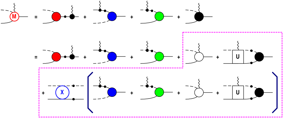
FIG. 1.: Meson production current $M^{\mu}$. Time proceeds from right to left. The first line, which sums up the $s$-, $u$-, and $t$-channel diagrams and the interaction current $M^{\mu}_{\rm int}$ (right-most diagram), is referred to as the tree-level. The dynamical content of $M^{\mu}_{\rm int}$, including the final-state interaction mediated by the nonpolar $\pi N$ amplitude $X$ (see Fig. 2), is explicitly shown by the diagrams enclosed in the dashed box. The diagram element labelled $U$ subsumes all exchange currents $U^{\mu}$ contributing to the process. The diagram with open circle depicts the bare current $m^{\mu}_{\rm bare}$.

Gauge invariance is one of the central issues when attempting to describe how photons interact with hadronic systems. Concentrating on the simplest case—pion photoproduction with real or virtual photons, gauge invariance can easily be shown to follow if the $\pi N$ and $\gamma N$ problems are treated completely and consistently on an equal footing [1, 2, 3, 4]. In practice, however, one often needs to revert to some approximate treatment of one or more of the contributing reaction mechanisms and this usually leads to a violation of gauge invariance. To restore it, the neglected reaction mechanisms must be approximated by auxiliary currents constructed such that the gauge-invariance-violating contributions to the four-divergence of the total production amplitude are cancelled. Such a procedure cannot be unique, of course, since one may always add arbitrary transverse currents without affecting the four-divergence.

At the tree-level, where one does not resolve the internal mechanisms entering the interaction current (cf. Fig. 1), various recipes exist to preserve gauge invariance. The simplest case concerns the choice of bare vertices with pseudovector coupling for the $\pi NN$ vertex, where the corresponding Kroll–Ruderman contact current [5] follows from the minimal substitution procedure. The case of extended nucleons, whose internal structure is described in terms of (phenomenological) form factors, is treated in Refs. [4, 6, 7, 8, 9].

In the present work, we want to go beyond the tree level and investigate how one can preserve gauge invariance if the internal structure of the interaction current is taken into account explicitly. The reaction mechanisms that enter the interaction current are summarized within the dashed box in Fig. 1. Specifically, we are interested in preserving gauge invariance in the explicit presence of hadronic final-state interactions. This is achieved by introducing auxiliary currents which cancel the gauge-invariance-violating contributions. In particular, we show how one may exploit the constraints following from the generalized Ward–Takahashi identities to construct these currents.

The present discussion is restricted to nucleons and pions only to facilitate the presentation. We do not include here possible resonances or other transition mechanisms since their couplings to the electromagnetic field are transverse and have no bearing on the question of gauge invariance. None of these restrictions are essential, however, and one may easily adapt the present formalism to accommodate more complex situations.

II Gauge Invariance

The pion photoproduction current of the nucleon is shown in Fig. 1 [4]. According to the diagrams in the first line of this figure, the total current $M^{\mu}$ may be broken up into four main contributions: The three Born terms due to the $s$-, $u$-, and $t$-channel currents stemming from the photon coupling to the three external legs of the $\pi NN$ vertex, and the interaction current $M^{\mu}_{\rm int}$ where the photon attaches itself to an internal leg of the $\pi NN$ vertex, i.e.,

$$M^{\mu}=M^{\mu}_{s}+M^{\mu}_{u}+M^{\mu}_{t}+M^{\mu}_{\rm int}\;.$$ (1)

While the first three contributions are relatively straightforward, the last one—as it is shown in the last two lines of Fig. 1—explicitly involves the full complexity of the internal reaction dynamics of the underlying $\pi N$ scattering problem summarized in Fig. 2.

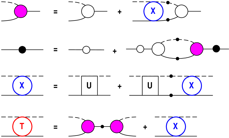
FIG. 2.: Pion-nucleon scattering with fully dressed hadrons. The full $\pi N$-amplitude is denoted by $T$, with $X$ subsuming all of its nonpolar (i.e., non-$s$-channel) contributions. The latter satisfies the Bethe–Salpeter-type integral equation depicted in the third line here, where the driving term $U$ sums up all nonpolar irreducible contributions to $\pi N$-scattering, i.e., all irreducible contributions which do not contain an $s$-channel pole (see Ref. [4] for full details). Diagram elements with open, unlabeled circles describe bare quantities.

For gauge invariance of the total current $M^{\mu}$ to hold true, its four-divergence must satisfy a generalized Ward–Takahashi identity [2, 3, 4]

$$k_{\mu}M^{\mu} = -[F_{s}\tau]S_{p+k}Q_{i}S^{-1}_{p}+S^{-1}_{p^{\prime}}Q_{f}S_{p^{\prime}-k}[F_{u}\tau]$$ (3)

$${}+\Delta^{-1}_{q}Q_{\pi}\Delta_{q-k}[F_{t}\tau]\;,$$

where $p$ and $k$ are the four-momenta of the incoming nucleon and photon, respectively, and $p^{\prime}$ and $q$ are the four-momenta of the outgoing nucleon and pion, respectively, related by momentum conservation $p^{\prime}+q=p+k$. $S$ and $\Delta$ are the propagators of the nucleons and pions, respectively, with their subscripts denoting the available four-momentum for the corresponding hadron; $Q_{i}$, $Q_{f}$, and $Q_{\pi}$ are the initial and final nucleon and the pion charge operators, respectively. $[F_{x}\tau]$ denotes the $\pi NN$ vertex (including coupling and isospin operators), with the subscript $x$ labeling the kinematic situation appropriate for the $s$-, $u$-, or $t$-channel diagrams appearing in Fig. 1. The vertex isospin $\tau$ does not commute with the charge operators and $\tau Q_{i}-Q_{f}\tau-Q_{\pi}\tau=0$ describes charge conservation at the vertex in a symbolic manner.

Equation (3) is easily obtained from Eq. (1) upon using the Ward–Takahashi identities [1] for the nucleon and pion currents,

$$k_{\mu}J^{\mu}_{\sc n} = S^{-1}_{p_{\sc n}+k}Q_{\sc n}-Q_{\sc n}S^{-1}_{p_{\sc n}}\;,$$ (5)

$$k_{\mu}J^{\mu}_{\pi} = \Delta^{-1}_{q_{\pi}+k}Q_{\pi}-Q_{\pi}\Delta^{-1}_{q_{\pi}}\;,$$ (6)

where $p_{\sc n}$ and $q_{\pi}$ are the respective initial hadron momenta of the electromagnetic vertices, and using the fact that for gauge invariance to be true the interaction current must obey [2, 4]

$$k_{\mu}M^{\mu}_{\rm int}=-[F_{s}\tau]Q_{i}+Q_{f}[F_{u}\tau]+Q_{\pi}[F_{t}\tau]\;.$$ (7)

A Preserving gauge invariance

As alluded to above, the preceding relations can easily be shown to be true if the $\pi N$ and $\gamma N$ problems are treated consistently on an equal footing [3, 4]. In practical applications, however, approximations are inevitable which usually violate the gauge invariance.

To see how one may preserve gauge invariance in such a situation, let us explicitly write the four-divergence of the interaction current using the relevant parts of Fig. 1 as guidance. One finds

$$k_{\mu}M^{\mu}_{\rm int} = k_{\mu}m^{\mu}_{\rm bare}+k_{\mu}U^{\mu}G_{0}[F\tau]$$ (10)

$${}+XG_{0}\Big{\{}k_{\mu}J^{\mu}_{\sc n}S_{p_{\sc n}-k}[F_{u}\tau]+k_{\mu}J^{\mu}_{\pi}\Delta_{q_{\pi}-k}[F_{t}\tau]$$

$${}\quad\quad+k_{\mu}m^{\mu}_{\rm bare}+k_{\mu}U^{\mu}G_{0}[F\tau]\Big{\}}\;,$$

where $G_{0}=S_{p_{\sc n}}\Delta_{q_{\pi}}$ denotes the product of the intermediate nucleon and pion propagators, with respective four-momenta $p_{\sc n}$ and $q_{\pi}$ denoting the integration variables, and $X$ is the nonpolar $\pi N$ amplitude (see Fig. 2) which mediates the hadronic final-state interaction; $U^{\mu}$ subsumes all exchange currents and $m^{\mu}_{\rm bare}$ is the bare contact current.

For gauge invariance to hold true, the bare current must satisfy the condition [4]

$$k_{\mu}m^{\mu}_{\rm bare}=-[f_{s}\tau]Q_{i}+Q_{f}[f_{u}\tau]+Q_{\pi}[f_{t}\tau]\;,$$ (11)

where $[f_{x}\tau]$ denotes the bare $\pi NN$ vertex the same way the notation $[F_{x}\tau]$ was used above for the dressed vertex. This is the analog of Eq. (7) for the bare current; it is usually satisfied as a matter of course. One of the simplest nontrivial examples is the case of pure pseudovector coupling without form factors, where $m^{\mu}_{\rm bare}$ is the Kroll–Ruderman contact current [5]; see Eq. (27).

Combining now Eq. (10) with the necessary condition (7), and making use of Eq. (11) in the Born terms, produces

$$0 = \Big{(}[F_{s}\tau]-[f_{s}\tau]\Big{)}Q_{i}-Q_{f}\Big{(}[F_{u}\tau]-f_{u}\tau]\Big{)}$$ (15)

$${}-Q_{\pi}\Big{(}[F_{t}\tau]-[f_{t}\tau]\Big{)}+k_{\mu}U^{\mu}G_{0}[F\tau]$$

$${}+XG_{0}\Big{\{}k_{\mu}J^{\mu}_{\sc n}S_{p_{\sc n}-k}[F_{u}\tau]+k_{\mu}J^{\mu}_{\pi}\Delta_{q_{\pi}-k}[F_{t}\tau]$$

$${}\quad\quad+k_{\mu}m^{\mu}_{\rm bare}+k_{\mu}U^{\mu}G_{0}[F\tau]\Big{\}}$$

as a necessary off-shell requirement for gauge invariance to be satisfied.

In other words, as long as the basic Ward–Takahashi identities (2) for the hadron currents are true, any approximation of the full reaction mechanisms constructed in such a manner that the condition (15) is satisfied will also preserve gauge invariance as a matter of course.

In view of the arbitrariness of transverse contributions, there are of course infinitely many ways this can be achieved. The prescription we give in the following applies to the simplifying assumption that one completely omits the explicit treatment of exchange currents $U^{\mu}$. However, even if they are taken into account in some partial manner, it is a straightforward exercise to adapt the following formulation to accommodate such situations.

Omitting explicit exchange currents, we maintain gauge invariance by constructing auxiliary currents $j^{\mu}_{0}$ and $j^{\mu}_{1}$ which provide the same effect as the exchange currents $U^{\mu}$ as far as the preservation of gauge invariance is concerned.

To this end, we make the replacements

$$U^{\mu}G_{0}[F\tau] \longrightarrow j^{\mu}_{0}+\Delta j^{\mu}_{0}\;,$$ (17)

$$XG_{0}U^{\mu}G_{0}[F\tau] \longrightarrow j^{\mu}_{1}+\Delta j^{\mu}_{1}\;,$$ (18)

and demand that $j^{\mu}_{0}$ and $j^{\mu}_{1}$ satisfy

$$k_{\mu}j^{\mu}_{0} = -\Big{(}[F_{s}\tau]-[f_{s}\tau]\Big{)}Q_{i}+Q_{f}\Big{(}[F_{u}\tau]-[f_{u}\tau]\Big{)}$$ (20)

$${}+Q_{\pi}\Big{(}[F_{t}\tau]-[f_{t}\tau]\Big{)}$$

and

$$k_{\mu}j^{\mu}_{1} = -XG_{0}\Big{\{}k_{\mu}J^{\mu}_{\sc n}S_{p_{\sc n}-k}[F_{u}\tau]+k_{\mu}J^{\mu}_{\pi}\Delta_{q_{\pi}-k}[F_{t}\tau]$$ (22)

$${}\quad\quad+k_{\mu}m^{\mu}_{\rm bare}\Big{\}}\;.$$

Clearly, if these conditions are met, then

$$k_{\mu}\left(\Delta j^{\mu}_{0}+\Delta j^{\mu}_{1}\right)=0\;,$$ (23)

i.e., $\Delta j^{\mu}_{0}+\Delta j^{\mu}_{1}$ is purely transverse. Without explicit treatment of exchange currents, these contributions are inaccessible and will be dropped. The resulting production current,

$$M^{\mu} = M^{\mu}_{s}+M^{\mu}_{u}+M^{\mu}_{t}+m^{\mu}_{\rm bare}+j^{\mu}_{0}$$ (25)

$${}+XG_{0}\Big{\{}M^{\mu}_{u}+M^{\mu}_{t}+m^{\mu}_{\rm bare}\Big{\}}+j^{\mu}_{1}\;,$$

will then satisfy the generalized Ward–Takahashi identity (3) and therefore it will be gauge invariant.

To be more specific as to how to implement the conditions (20) and (22), allowing for a mixture of pseudoscalar and pseudovector couplings, let us write the dressed $\pi NN$ vertex as

$$F=g_{\rm ps}\gamma_{5}G_{\rm ps}+g_{\rm pv}\frac{\gamma_{5}q\!\!\!/_{\pi}}{2m}G_{\rm pv}\;,$$ (26)

where the indices ps and pv stand for pseudoscalar and pseudovector contributions, respectively; $G_{\rm ps}$ and $G_{\rm pv}$ denote the corresponding normalized form factors (with their strength parameters $g_{\rm ps}$ and $g_{\rm pv}$ adding up to the physical coupling constant, $g_{\pi NN}=g_{\rm ps}+g_{\rm pv}$), $q_{\pi}$ is the four-momentum of the pion, and $m$ the nucleon mass. The bare vertex $f$ is given by the same equation with all $G$’s removed, and the corresponding bare current,

$$m^{\mu}_{\rm bare}=-g_{\rm pv}\frac{\gamma_{5}\gamma^{\mu}}{2m}Q_{\pi}\tau\;,$$ (27)

is just the usual Kroll–Ruderman contact term [5].

Equation (20) now reads explicitly

$$k_{\mu}j^{\mu}_{0} = -\gamma_{5}\Big{(}G_{s}-g\Big{)}\tau Q_{i}$$ (32)

$${}+\gamma_{5}\Big{(}G_{u}-g\Big{)}Q_{f}\tau$$

$${}+\gamma_{5}\Big{(}G_{t}-g\Big{)}Q_{\pi}\tau$$

$${}-g_{\rm pv}\gamma_{5}\frac{k\!\!\!/}{2m}\Big{(}G_{{\rm pv},s}\tau Q_{i}-G_{{\rm pv},u}Q_{f}\tau\Big{)}$$

$${}-k_{\mu}m^{\mu}_{\rm bare}\;,$$

where

$$G_{x}=g_{\rm ps}G_{{\rm ps},x}+g_{\rm pv}\frac{p\!\!\!/-p\!\!\!/^{\prime}}{2m}G_{{\rm pv},x}$$ (33)

(with $x=s$, $u$, $t$) denotes the kinematic situations in which the vertex functions $G_{\rm ps}$ and $G_{\rm pv}$ appear; $g$ is given by the same equation with all $G$’s removed.

Note that all the terms containing $g$ in Eq. (32) add up to zero. We may therefore replace $g$ by an arbitrary function $\widehat{F}$ with impunity. Furthermore, using the Mandelstam variables $s=(p+k)^{2}$, $u=(p^{\prime}-k)^{2}$, and $t=(q-k)^{2}$, we may then rewrite the resulting equation as

$$k_{\mu}j^{\mu}_{0} = k_{\mu}\Bigg{\{}-\frac{(2p+k)^{\mu}}{s-p^{2}}\gamma_{5}\Big{(}G_{s}-\widehat{F}\Big{)}\tau Q_{i}$$ (38)

$${}\quad\quad-\frac{(2p^{\prime}-k)^{\mu}}{u-p^{\prime 2}}\gamma_{5}\Big{(}G_{u}-\widehat{F}\Big{)}Q_{f}\tau$$

$${}\quad\quad-\frac{(2q-k)^{\mu}}{t-q^{2}}\gamma_{5}\Big{(}G_{t}-\widehat{F}\Big{)}Q_{\pi}\tau$$

$${}\quad\quad-g_{\rm pv}\frac{\gamma_{5}\gamma^{\mu}}{2m}\Big{(}G_{{\rm pv},s}\tau Q_{i}-G_{{\rm pv},u}Q_{f}\tau\Big{)}$$

$${}\quad\quad-m^{\mu}_{\rm bare}\Bigg{\}}\;,$$

which allows us to put

$$j^{\mu}_{0} = -\frac{(2p+k)^{\mu}}{s-p^{2}}\gamma_{5}\Big{(}G_{s}-\widehat{F}\Big{)}\tau Q_{i}$$ (42)

$${}-\frac{(2p^{\prime}-k)^{\mu}}{u-p^{\prime 2}}\gamma_{5}\Big{(}G_{u}-\widehat{F}\Big{)}Q_{f}\tau$$

$${}-\frac{(2q-k)^{\mu}}{t-q^{2}}\gamma_{5}\Big{(}G_{t}-\widehat{F}\Big{)}Q_{\pi}\tau$$

$${}-g_{\rm pv}\frac{\gamma_{5}\gamma^{\mu}}{2m}\Big{(}G_{{\rm pv},s}\tau Q_{i}-G_{{\rm pv},u}Q_{f}\tau\Big{)}-m^{\mu}_{\rm bare}\;.$$

Comparing with Eq. (25), note that the last two terms of this gauge-invariance-preserving current cancel the bare Kroll–Ruderman term and replace it by a dressed one, where instead of the pion charge $Q_{\pi}\tau$, there is now a dressing term $G_{{\rm pv},s}\tau Q_{i}-G_{{\rm pv},u}Q_{f}\tau$. This dressing term expresses the pion charge in terms of the nucleon charges modified by hadronic form factors, and, in general, it will be non-zero even if the pion is uncharged.

We emphasize that the transition from Eq. (32) to (42) is not unique, of course, since one may add a divergence-free current to $j^{\mu}_{0}$ without changing the necessary condition (32). In fact, the replacement of $g$ by $\widehat{F}$ amounts to the addition of such a transverse current (which in turn may be understood as a phenomenological way of getting a handle on the neglected transverse current $\Delta j^{\mu}_{0}+\Delta j^{\mu}_{1}$). At this stage, $\widehat{F}$ is completely undetermined. Below, when considering the relationship of the present results to existing tree-level approaches, we will discuss some specific choices.

We also note that the terms appearing in Eq. (42) do not introduce any new singularities into the amplitude. This is easily illustrated for the example of the $s$-channel pole diagram $M^{\mu}_{s}$, viz.

$$M^{\mu}_{s} = [F_{s}\tau]\frac{p\!\!\!/+k\!\!\!/+m}{s-m^{2}}\gamma^{\mu}Q_{i}+M^{\mu}_{{\sc t},s}$$ (43)

$$= \gamma_{5}G_{s}\frac{(2p+k)^{\mu}}{s-m^{2}}\tau Q_{i}+g_{\rm pv}\frac{\gamma_{5}k\!\!\!/}{2m}G_{{\rm pv},s}\frac{(2p+k)^{\mu}}{s-m^{2}}\tau Q_{i}$$ (45)

$${}+\gamma_{5}G_{s,q\!\!\!/}\frac{k^{\mu}-\gamma^{\mu}k\!\!\!/}{s-m^{2}}\tau Q_{i}+M^{\mu}_{{\sc t},s}\;,$$

where $G_{s,q\!\!\!/}$ is given by Eq. (33) with $p\!\!\!/-p\!\!\!/^{\prime}$ replaced by $q\!\!\!/$; $M^{\mu}_{{\sc t},s}$ splits off the transverse part of the electromagnetic nucleon current given in Eq. (50) below. The decomposition given here makes it immediately obvious that the effect of adding the $s$-channel term, with $p^{2}=m^{2}$, of Eq. (42) to this expression is to replace $G_{s}$ in the first term here by $\widehat{F}$. The same happens also for the $u$- and $t$-channel diagrams. In other words, apart from providing a dressed Kroll–Ruderman term, the effect of the gauge-invariance preserving current (42) is to provide a common form factor $\widehat{F}$ for some (but not all) of the contributions originally containing individual form factors $G_{s}$, $G_{u}$, and $G_{t}$, without changing the original singularities of the Born diagrams.

Next, to construct the current $j^{\mu}_{1}$, we recall that the gauge-invariant nucleon and pion currents appearing in the $u$- and $t$-channel terms of the final-state interaction contribution are given by

$$J^{\mu}_{\sc n} = \gamma^{\mu}Q_{\sc n}+J^{\mu}_{{\sc t},{\sc n}}\;,$$ (47)

$$J^{\mu}_{\pi} = (2q_{\pi}-k)^{\mu}Q_{\pi}+J^{\mu}_{{\sc t},\pi}\;,$$ (48)

respectively, with transverse pieces which follow from demanding the validity of the Ward–Takahashi identities (2), i.e.,

$$J^{\mu}_{{\sc t},{\sc n}} = \left(\gamma^{\mu}-k^{\mu}\frac{k\!\!\!/}{k^{2}}\right)Q_{\sc n}(F_{1}-1)+i\frac{\sigma^{\mu\nu}k_{\nu}}{2m}\kappa F_{2}\;,$$ (50)

$$J^{\mu}_{{\sc t},\pi} = \left[(2q_{\pi}-k)^{\mu}-k^{\mu}\frac{k\cdot(2q_{\pi}-k)}{k^{2}}\right]Q_{\pi}(F_{\pi}-1)\;,$$ (51)

where $F_{1}$ and $F_{2}$ respectively are the electromagnetic Dirac and Pauli form factors of the nucleon, with $\kappa$ being its anomalous magnetic moment, and $F_{\pi}$ is the electromagnetic form factor of the pion. Their four-divergence is given by

$$k_{\mu}J^{\mu}_{\sc n} = k_{\mu}\gamma^{\mu}Q_{\sc n}\;,$$ (54)

$$k_{\mu}J^{\mu}_{\pi} = k_{\mu}(2q_{\pi}-k)^{\mu}Q_{\pi}\;.$$ (55)

Inserting this into Eq. (22), we may then extract the gauge-invariance-preserving current as

$$j^{\mu}_{1} = -XG_{0}\Big{\{}\gamma^{\mu}Q_{\sc n}S_{p_{\sc n}-k}[F_{u}\tau]$$ (57)

$${}\quad\quad+(2q_{\pi}-k)^{\mu}Q_{\pi}\Delta_{q_{\pi}-k}[F_{t}\tau]+m^{\mu}_{\rm bare}\Big{\}}\;.$$

Its effect on the final-state interaction part of the production amplitude (25) is seen to simply cancel the bare current and to reduce the $u$- and $t$-channel contributions to their respective transverse pieces, i.e.,

$$XG_{0}\Big{(}M^{\mu}_{{\sc t},u}+M^{\mu}_{{\sc t},t}\Big{)} = XG_{0}\Big{\{}M^{\mu}_{u}+M^{\mu}_{t}+m^{\mu}_{\rm bare}\Big{\}}+j^{\mu}_{1}$$ (58)

$$= {}XG_{0}\Big{\{}J^{\mu}_{{\sc t},{\sc n}}S_{p_{\sc n}-k}[F_{u}\tau]$$ (60)

$${}\quad\quad+J^{\mu}_{{\sc t},\pi}\Delta_{q_{\pi}-k}[F_{t}\tau]\Big{\}}\;.$$

The entire contribution from the final-state interaction, therefore, is purely transverse.

B Relation to Ohta’s and Haberzettl’s tree-level prescriptions

To make the connection with tree-level approaches, we need to switch off all final-state interactions and put $X=0$ in Eqs. (22) and (25). The conditions to be satisfied, therefore, are Eq. (20) and Eq. (22) in the form

$$k_{\mu}j^{\mu}_{1}=0\;.$$ (61)

In other words, simply putting $j^{\mu}_{1}=0$ satisfies all gauge-invariance constraints at the tree level.

Both Ohta’s [7] and Haberzettl’s [4, 9] prescriptions for preserving gauge invariance can be understood as different choices for the function $\widehat{F}$ in Eq. (42).

Ohta’s approach, based on a particular application of the minimal substitution procedure, finds

$$\widehat{F}=g_{\rm ps}G_{\rm ps}(q,p^{\prime},p)+g_{\rm pv}\frac{p\!\!\!/-p\!\!\!/^{\prime}}{2m}G_{\rm pv}(q,p^{\prime},p)\;,$$ (62)

where the external hadron momenta of the photoproduction current—a four-point function—appear here as the momenta of the $\pi NN$ vertex—a three-point function. Since the momenta satisfy $q+p^{\prime}=p+k$, this mismatch corresponds to an unphysical region of the $\pi NN$ vertex (which leads to the problems discussed in Ref. [10]). Only in the infrared limit of $k=0$, this mismatch is resolved and then this choice prevents the current (42) from being singular at $k=0$.

In Haberzettl’s prescription, the function $\widehat{F}$ is a linear combination of the three kinematical situations in which the $\pi NN$ vertices appear in the Born terms, i.e., [cf. Eq. (33)]

$$\widehat{F}=a_{s}G_{s}+a_{u}G_{u}+a_{t}G_{t}\;,$$ (63)

with coefficients constrained by $a_{s}+a_{u}+a_{t}=1$, which may be fixed according to prejudice or used as free fit parameters. In contrast to Ohta’s choice, this does not require any unphysical values for the $\pi NN$ form factors in practical applications, and it also has a well-behaved infrared limit. In direct comparisons to Ohta’s, this prescription is found to provide better agreement with the experimental data [9, 11, 12] .

III Summary and Discussion

In summary, we have treated here the electromagnetic production current for mesons off the nucleon for both real and virtual photons. We used the constraints following from requiring the validity of the generalized Ward–Takahashi identities to construct auxiliary current pieces that ensure that gauge invariance is preserved even if—as it is invariably the case in practical applications—one does not treat the problem completely and consistently. The result for the production current $M^{\mu}$ obtained here in Eqs. (25), (42), and (57) can be summarized by

$$M^{\mu} = M^{\mu}_{s}+M^{\mu}_{u}+M^{\mu}_{t}+j^{\mu}_{\sc gip}$$ (65)

$${}+XG_{0}\Big{(}M^{\mu}_{{\sc t},u}+M^{\mu}_{{\sc t},t}\Big{)}\;,$$

where the gauge-invariance-preserving current,

$$j^{\mu}_{\sc gip}=j^{\mu}_{0}+m^{\mu}_{\rm bare}\;,$$ (66)

is given via $j^{\mu}_{0}$ of Eq. (42).

As far as the choice of the function $\widehat{F}$ appearing in $j^{\mu}_{0}$ is concerned, the generally better results obtained with Haberzettl’s prescription at the tree-level [9, 11, 12] seem to favor the form given in Eq. (63). We emphasize, however, that other functions are possible and that, in general, as far as gauge invariance is concerned, any current $j^{\mu}_{0}$ that satisfies the necessary condition (32) is permitted here.

The part describing the hadronic final-state interaction due to $X$ does no longer contain the Kroll–Ruderman contact term since it is canceled by the current of Eq. (57). Moreover, what remains is seen to be entirely transverse since the corresponding $u$- and $t$-channel contributions, $M^{\mu}_{{\sc t},u}$ and $M^{\mu}_{{\sc t},t}$, respectively contain only the transverse electromagnetic nucleon and pion operators of Eq. (II A). For real photons, in particular, both $F_{\pi}-1$ and $F_{1}-1$ vanish and therefore $M^{\mu}_{{\sc t},t}=0$, i.e., the $t$-channel does not contribute at all, and the $u$-channel current $M^{\mu}_{{\sc t},u}$ is reduced to the magnetic $\sigma^{\mu\nu}k_{\nu}$ term from Eq. (50).

We emphasize that even though the gauge-invariant production current of Eq. (65) is an approximation to the full dynamics of the problem as summarized in Figs. 1 and 2, it is complete as far as the longitudinal components of the current are concerned. Any additional pieces must be transverse.

Let us repeat once again that the present work was restricted to pions and nucleons merely to simplify the presentation. The concepts developed here are quite general, however. An extension to other baryons and mesons, therefore, is straightforward and easily done along the lines given here. In particular, the fact that the final-state interaction contributions are purely transverse remains true if one takes into account additional intermediate hadrons ($\Delta$, $\rho$, etc.) since, just as was demonstrated here for the nucleons and pions, only the transverse parts of their respective current operators survive in the final-state interaction terms.

Finally, let us point out that the present results remain equally valid whether the form factors $F$ and the final-state amplitude $X$ are obtained via some sophisticated Bethe–Salpeter-type formalism or are based on a simple phenomenological model ansatz. How these elements are obtained does not enter any of the present considerations and therefore has no bearing on the question of gauge invariance.

- [1] J. C. Ward, Phys. Rev. 78, 182 (1950); Y. Takahashi, Nuovo Cimento 6, 371 (1957).
- [2] E. Kazes, Nuovo Cimento 13, 1226 (1959).
- [3] C. H. M. van Antwerpen and I. R. Afnan, Phys. Rev. C 52, 554 (1995).
- [4] H. Haberzettl, Phys. Rev. C 56, 2041 (1997).
- [5] N. M. Kroll and M. A. Ruderman, Phys. Rev. 93, 233 (1954).
- [6] F. Gross and D. O. Riska, Phys. Rev. C 36, 1928 (1987).
- [7] K. Ohta, Phys. Rev. C 40, 1335 (1989).
- [8] S. I. Nagorny et al., Sov. J. Nucl. Phys. 49, 465 (1989); 53, 228 (1991); 55, 1325 (1992).
- [9] H. Haberzettl, C. Bennhold, T. Mart, and T. Feuster, Phys. Rev. C 58, R40, (1998).
- [10] S. Wang and M. K. Banerjee, Phys. Rev. C 54, 2883 (1996).
- [11] T. Feuster and U. Mosel, Phys. Rev. C 59, 460 (1999).
- [12] B. S. Han, M. K. Cheoun, K. S. Kim, and I.-T. Cheon, Los Alamos Eprint nucl-th/9912011.