Pion-nucleon interaction in a covariant hadron-exchange model

Abstract

We develop a relativistic covariant and unitary description of the pion-nucleon interaction in a hadron-exchange model. The model is based on the solution of a dimensionally reduced (quasipotential) Bethe-Salpeter equation for the partial-wave off-shell $\pi N$ scattering amplitudes with the potential consisting of the field-theoretical $s$- and $u$-channel nucleon, Roper, Delta, $D_{13}$, $S_{11}$ exchanges, and the $t$-channel $\rho$ and $\sigma$ meson exchanges. The contributions of the spin-3/2 Delta and $D_{13}$ resonances are treated within the Rarita-Schwinger formalism and different forms of the $\pi N\Delta$ vertex are investigated. The free parameters of the model are fitted to the $\pi N$ phase-shift data of the KH80 and SM95 partial-wave analyses in the region up to 600 MeV pion kinetic energy. The resulting on-shell solution provides a good description of the $\pi N$ scattering lengths, as well as the energy behavior of the S, P, and D partial waves. The sensitivity of the phase shifts on various model-dependent effects is examined.

I Introduction

The $\pi N$ interaction received much attention in the past both theoretically and experimentally in view of its fundamental nature (early literature can be found in Refs. [1, 2]). Current theoretical interest is triggered by the experimental programs being carried out at NIKHEF, MAMI, TJNAF and other intermediate-energy facilities with the purpose to understand the structure of hadrons and their interaction in the confinement region of QCD. To extract most physics from the new high-precision measurements a reliable and accurate knowledge of $\pi N$ and $NN$ interaction is required. Highly successful attempts have been made in describing these interactions in terms of hadronic degrees of freedom over a wide energy region. In particular, the relativistic one-boson-exchange models were successfully applied to the description of $NN$ interaction, and especially during the past decade this theoretical framework has been extended to the $\pi N$ system [3, 4, 5, 6, 7, 8, 9, 10]. Such an extension gives one a capability to study a broad class of reactions, including pion scattering and production on light nuclei in a self-consistent framework. In this paper we report on a relativistic covariant $\pi N$ model using the quasipotential approach and based on an effective interaction characterized by a hadron-exchange potential (some of our results have already been briefly reported [10, 11]).

Although the underlying dynamics of the $\pi N$ interaction is nowadays believed to be governed by QCD, it is practically impossible to resolve it fully in terms of quarks and gluons because of the confinement problem. Much of the present understanding of the $\pi N$ physics at low and intermediate energies remains to be based on dispersion relations [2] and effective chiral Lagrangians [12, 13] in term of the hadron degrees of freedom.

The chiral pion-nucleon Lagrangians are usually extended in two ways: first, by including higher-mass states, such as $\rho$-meson, $\Delta$-isobar, etc.; secondly, by including the higher-derivative terms. Both ways are necessary to extend such a phenomenological description to higher energies: The contributions due to higher-mass states have a clear physical significance, while the higher-derivative terms are needed to examine the effect of unknown short-range physics. The higher-derivative terms play, for instance, a crucial role in the renormalization program of chiral perturbation theory (ChPT). In the hadron-exchange models, a similar role is played by the “strong form factors” which are included in the effective Lagrangian to model the short distance behavior of the potential. Both ChPT and hadron-exchange models thus begin from a similar “extended” chiral Lagrangian but the approach to calculating the $\pi N$ scattering amplitude is somewhat different. In ChPT one usually performs a perturbative field-theoretic calculation maintaining crossing-symmetry and exact agreement with the soft-pion theorems. (For the development of ChPT in application to the $\pi N$ scattering see Ref. [14].) In the hadron-exchange approach one uses the effective Lagrangian to construct the potential which then is resumed via a scattering equation. In this way crossing symmetry is given up in favor of exact unitarity in a given channel space, and possibility of studying nonperturbative phenomena such as dynamical resonances.

In defining a hadron-exchange model one usually specifies three ingredients: effective Lagrangian, potential, and the scattering equation. These ingredients are interrelated in quantum field theory, where one must solve the Bethe-Salpeter (BS) equation and has a well-determined procedure for computing its kernel from a given Lagrangian. The BS kernel consists of all the irreducible graphs and hence can be computed only perturbatively. In this work we shall take the potential to be given by the tree-level graphs, although we do not claim that the used Lagrangian justify any perturbative expansion. On the other hand, the resulting approximation transparently relates to the usual quantum-mechanical picture where the scattering problem is given by a Lippmann-Schwinger type of equation for one-particle exchange potentials. Therefore, one might prefer to view this approach as relativistic quantum-mechanical one rather than some “nonsystematic” truncation of QFT.

The four-dimensional BS equation for the $\pi N$ system (with a one-particle-exchange potential) has been solved by Nieland and Tjon [15], and recently by Lahiff and Afnan [9] in a more realistic setup. Models [3, 5, 7, 10] exploit instead various quasipotential (QP) equations, which can be obtained by a three-dimensional reduction of the BS equation. The use of QP equations provides a technical simplification of the problem, without destroying the Lorentz invariance of the theory. It should be remarked, however, that some of the QP equations can violate charge conjugation symmetry, and because this symmetry is crucial for renormalizing the positive- and negative-energy baryon poles in an equivalent way, the equations which violate it are less preferable. We will employ the equal-time (ET) equation which preserves the full Lorentz covariance, including charge conjugation. This equation will be specified in the next section.

Apart from the technical simplifications, the QP approach can sometimes be motivated by physical arguments. For instance, while the four-dimensional BS equation for $t$-channel (meson-exchange) potential, i.e., the ladder BS equation, has a wrong one-body limit, a number of QP equations with the proper limit can be devised [16, 17, 18, 19]. In the $\pi N$ situation the potential may, in addition to the $t$-channel meson exchanges, contain the $u$-channel baryon exchanges, which spoil the standard one-body limit arguments [20]. The ordinary ET equation is shown to provide an optimal choice in the case when both $t$- and $u$-channel exchanges are present in the force corresponding to the $\pi N$ situation[20].

As for the effective Lagrangian, we use the pseudovector $\pi NN$ coupling, and include $\sigma$, $\rho$ mesons, and all the relevant (for the considered energy region) nucleon resonances as explicit degrees of freedom. The precise form of the Lagrangian and the potential is discussed in Sec. IV. An interesting aspect, which comes in with the nonperturbative modelling, is that for a sufficiently attractive potential the nucleon resonances can be generated dynamically, as quasi-bound states of the $\pi N$ system. In models [15, 21] and quantum hadrodynamics [22] the $\Delta$(1232) is described in this way. Lahiff and Afnan [9] include the $\Delta$ explicitly, but suggest that the Roper resonance can be of dynamical origin. Gross and Surya [5] include the $\Delta$ and the Roper poles, but treat the $S_{11}$ resonance dynamically. In this paper we consider $P_{33}\,\Delta$(1232), $P_{11}\,N^{\ast}$(1450), $D_{13}\,N^{\ast}$(1520), and $S_{11}\,N^{\ast}$(1535) resonances. Within our model, these resonances are all of nondynamical origin, i.e., are included explicitly via an effective Lagrangian description. Of course, the dynamical effects will anyhow contribute to the generation of the resonances seen in the phase-shifts. Thus, an admixture of both “elementary” and “composite” component constitutes the full result. Since the “elementary” fields corresponding to the resonances are included with real masses, the dynamical contributions are fully responsible for generating the width. Our model maintains the elastic $\pi N$ unitarity and therefore only the one-pion decay width of the resonances is generated.

As we have to deal with the spin-3/2 fields of resonances, such as that of the $\Delta$-isobar, we shall address here some of the problems of consistent formulation for relativistic higher-spin fields. Consistent formulations for the free spin-3/2 field have of course been known for a long time. The Rarita-Schwinger formalism [23] based on the vector-spinor field representation became the most popular one. The form of the free spin-3/2 action is uniquely (up to trivial field redefinitions) constrained by requirements of Poincaré invariance and consistent degrees-of-freedom counting. The latter requirement essentially means that the action must have enough symmetries to kill off the unphysical lower-spin components, and maintain only the physical $2s+1$ degrees-of-freedom of the theory. An arbitrarily constructed interaction may violate this consistency and activate the unphysical degrees of freedom. This necessarily leads to a number of pathologies, such as acausal propagations[24, 25], inadmissible quantization[26, 27], violation of Poincaré invariance.

The conventional $\pi N\Delta$ coupling[28, 29, 2] is an example of such pathological interactions. The contribution of the unphysical spin-1/2 components appear in the scattering amplitudes via the dependence on the so-called “off-shell parameter” and “spin-1/2 backgrounds.” On the other hand, a class of consistent $\pi N\Delta$ and $\gamma N\Delta$ couplings has recently been established [30, 31]. Those are essentially all possible couplings that maintain the gauge symmetry of the free massless Rarita-Schwinger action. In the present model we shall use the leading “gauge-invariant” $\pi N\Delta$ coupling, which has the same non-relativistic limit as the conventional one. In Sec. V we study the differences between the conventional and the gauge-invariant $\pi N\Delta$ coupling at the tree-level $\Delta$-exchange contributions. The largest differences are seen first of all in the spin-1/2 partial waves, where the conventional coupling gives the background contributions verse no contribution from the consistent couplings.

The parameters of the effective Lagrangian, including the form factor masses, form the set of model parameters. Some of them, such as the $\pi NN$ coupling constant, the nucleon, and the meson masses, are very well-determined elsewhere and therefore are kept fixed during the fits. The others are fitted to give the best agreement with the $\pi N$ partial-wave analyses [32, 33, 34]. The complete model provides an accurate description of the $S$- and $P$-wave scattering lengths ($\chi^{2}/{\rm datapoint}\simeq 1.4$), as well as the energy behavior of the $S$-, $P$-, and some of the $D$-wave phase-shifts up to 600 MeV pion lab kinetic energy.

In the next section we describe the covariant quasipotential equation for the off-shell $\pi N$ amplitudes, and its partial-wave decomposition. This will specify the equation solved in the model. In Sec. III we briefly discuss the effective Lagrangian used to read off the tree-level potential—the driving force of the equation. The renormalization procedure to treat the s-channel poles is described in Sec. IV. In Sec. V we analyze the effects of the different exchange contributions in the low-energy $\pi N$ data, and then present the results of the complete model emphasizing the effect of the rescattering contributions. Some discussion and concluding remarks are given in Sec. VI. Finally, various appendices contain some technical details of the analysis. In Appendix A we summarize the conventions. Appendix B shows some details of the partial-wave and isospin decomposition of the off-shell $\pi N$ amplitudes. Appendix C provides explicit expressions for various hadron-exchange contributions to the off-shell $\pi N$ potential. Amplitudes for higher-spin baryon exchange are discussed in Appendix D.

II Quasipotential approach

The fully off-shell relativistic $\pi N$ scattering amplitude in the space of the nucleon helicity spinors is described by sixteen scalar amplitudes: one for each combination of the helicity and $\rho$-spin of the initial and final nucleon. Parity conservation reduces the number of independent scalar amplitudes to eight. As a suitable covariant representation which expresses the off-shell amplitude in terms of eight invariants we choose the following:

$$T_{\lambda^{\prime}\lambda}^{\rho^{\prime}\rho}(p^{\prime},k^{\prime};p,k)=\bar{u}_{\lambda^{\prime}}^{\rho^{\prime}}(\vec{p}^{\prime})\,(1,p\!\!\!/^{\prime})\left[\left(\begin{array}[]{cc}A_{11}&A_{12}\\ A_{21}&A_{22}\end{array}\right)+P\!\!\!\!/\left(\begin{array}[]{cc}B_{11}&B_{12}\\ B_{21}&B_{22}\end{array}\right)\right]\left(\begin{array}[]{c}1\\ p\!\!\!/\end{array}\right)\,u_{\lambda}^{\rho}(\vec{p}),$$ (1)

where $A_{ij}$ and $B_{ij}$ are the eight scalar functions of invariants formed by the momenta, i.e., $p^{2}$, $p\cdot p^{\prime}$, etc. The four-momenta of the initial (final) nucleon and pion are given by $p$ and $k$ ($p^{\prime}$ and $k^{\prime}$), respectively, while $P$ is the conserved total four-momentum of the system:

$$P=p+k=p^{\prime}+k^{\prime}\,.$$

Due to the momentum conservation only three of the external momenta are independent, below we usually work with $p$, $p^{\prime}$ and $P$. Furthermore, $u_{\lambda}^{\rho}$ are the nucleon helicity spinors, where $\lambda=\pm\mbox{{$\frac{1}{2}$}}$ and $\rho=\pm 1$ ($\lambda^{\prime}$ and $\rho^{\prime}$) are the initial (final) helicity and $\rho$-spin of the nucleon, respectively.

For the on-shell situation ($p^{2}={p^{\prime}}^{2}=m_{N}^{2}$, $k^{2}={k^{\prime}}^{2}=m_{\pi}^{2}$) the amplitude reduces to the standard form [35]:

$$T_{\lambda^{\prime}\lambda}(p^{\prime},p;P)=\bar{u}_{\lambda^{\prime}}^{(+)}(\vec{p}^{\prime})\,\left[\hat{A}(s,t)+\mbox{{$\frac{1}{2}$}}\gamma\cdot(k^{\prime}+k)\,\hat{B}(s,t)\right]\,u_{\lambda}^{(+)}(\vec{p}),$$ (2)

[$s=P^{2},\,t=(p-p^{\prime})^{2},\,u=(p-k^{\prime})^{2}$ are the Mandelstam invariants]. We find from Eqs. (1) and (2)

$$\hat{B} = B_{11}+m_{N}(B_{12}+B_{21})+m_{N}^{2}B_{22},$$ (3)

$$\hat{A} = m_{N}\hat{B}+A_{11}+m_{N}(A_{12}+A_{21})+m_{N}^{2}A_{22}.$$ (4)

Our starting point for the $\pi N$ amplitude is the Bethe-Salpeter (BS) equation, schematically shown in Fig. 1,

$$T(p^{\prime},p)=V(p^{\prime},p)+i\int\!\frac{{\rm d}^{4}q}{4\pi^{3}}\,V(p^{\prime},q)\,G(q)\,T(q,p),$$ (5)

where $V$ is the potential, $G$ is the $\pi N$ propagator; the dependence on the total momentum $P$ is omitted. If $q$ is the relative four-momentum of the intermediate $\pi N$ state, the $\pi N$ propagator takes the following form:

$$G(q)=\frac{1}{(\beta P-q)^{2}-m_{\pi}^{2}+i\varepsilon}\,\frac{(\alpha P+q)\cdot\gamma+m_{N}}{(\alpha P+q)^{2}-m_{N}^{2}+i\varepsilon},$$ (6)

where

$$\alpha\equiv\alpha(s)=p\cdot P/s=(s+m_{N}^{2}-m_{\pi}^{2})/2s,$$ (7)

$$\beta\equiv\beta(s)=k\cdot P/s=(s-m_{N}^{2}+m_{\pi}^{2})/2s.$$ (8)

In approximating the BS equation one often simplifies the singularity structure of the kernel $VG$, such that the temporal integration can easily be done. This procedure is called three-dimensional (3D) reduction while the resulting equation is a quasipotential (QP) equation. For instance, in the reduction to the spectator equation [16, 5] all the poles of $V$ and the negative-energy pole of $G$ in the $q_{0}$ plane are neglected.

As we have recently emphasized [10, 11], the danger of doing a 3D reduction via approximating the pole structure is that the charge conjugation symmetry can be destroyed. In particular, in our naive interpretation of the spectator equation this symmetry is violated, essentially because of an asymmetric treatment of the positive- and negative-energy states. Gross has recently presented an interpretation of the spectator prescription which is consistent with the charge conjugation symmetry [36].

The equal-time (ET) reductions (see, e.g. [37]), such as Salpeter’s instantaneous approximation [38], preserve charge conjugation symmetry. In these reductions one effectively removes the $q_{0}$ poles from the potential while treating exactly the poles of the two-particle propagator $G$. To remove the potential poles one fixes the relative-energy variable $q_{0}$ in some way. Most frequently the constraint $q_{0}=0$, or its covariantized form: $P\cdot q=0$, is used.

We will be using the ET type of approach. To implement the constraint $P\cdot q=0$, we may impose the condition that the interaction is insensitive to the off-shellness along the direction defined by an unit four-vector $n_{\mu}$. For the two-body case this means that $V$ and $T$ entering the scattering equation depend on the projections of the relative four-vectors onto a 3D hyperplane orthogonal to $n_{\mu}$. Defining the projection operator,

$$O_{\mu\nu}={\rm g}_{\mu\nu}-n_{\mu}n_{\nu},$$ (9)

we write the corresponding equation as follows:

$$T(\tilde{l}^{\prime},\tilde{l})=V(\tilde{l}^{\prime},\tilde{l})+i\int\,\frac{{\rm d}^{4}q}{4\pi^{3}}\,V(\tilde{l}^{\prime},\tilde{q})\,G(q)\,T(\tilde{q},\tilde{l}),$$ (10)

where $l,\,l^{\prime},\,q$ are the relative momenta of the initial, final, and intermediate $\pi N$ state, respectively; $\tilde{l}_{\mu}=O_{\mu\nu}l^{\nu}$, and similarly for $\tilde{l}^{\prime},\,\tilde{q}$.

Equation (10) is manifestly covariant. On the other hand, it can easily be reduced to the 3D form. For instance, we can choose the frame where $n=(1,0,0,0)$, and therefore $V$ and $T$ are independent of the 0-th component of relative momenta (since any scalar product will depend only on the spatial components, e.g., $\tilde{q}\cdot\gamma=-\vec{q}\cdot\vec{\gamma}$). The integration over $q_{0}$ in Eq. (10) can now be readily done leading to the 3D equation. To prevent the dependence of the $S$-matrix on $n$, one may choose $n$ along some physical four-momentum, for instance along the total momentum: $n_{\mu}=P_{\mu}/\sqrt{P^{2}}.$ Then the reduction is possible in the center-of-mass system (CMS) where $P=(P_{0},0,0,0)$.

In the ET approach, the two-particle propagator is sometimes modified to include approximately the crossed graphs [18, 39], thus providing the correct one-body limit of the equation in the case of $t$-channel type of potential. We however do not apply such modifications here, because they actually worsen the predictions for the $\pi N$ case where the $u$-channel exchanges are present [20].

Because of rotational invariance and parity conservation it is convenient to partial-wave decompose Eqs. (5) and (10) (see Appendix B). Let

$$T_{\lambda^{\prime}\lambda}^{\rho^{\prime}\rho}(p^{\prime},p)=\sum\nolimits_{J}(J+\mbox{{$\frac{1}{2}$}})D^{J}_{\lambda^{\prime}\lambda}(\Omega_{p^{\prime}p})\,T_{\lambda^{\prime}\lambda}^{J\rho^{\prime}\rho}(p_{0}^{\prime},{\rm p}^{\prime},p_{0},{\rm p};P_{0}),$$ (11)

where $\Omega_{p^{\prime}p}$ is the solid angle between $\vec{p}^{\prime}$ and $\vec{p}$. Furthemore, in the CMS, using Eq. (1) and the Dirac equation

$$(p\!\!\!/-\rho m_{N})\,u_{\lambda}^{\rho}(\vec{p})=(p_{0}-\rho E_{p})\gamma_{0}\,u_{\lambda}^{\rho}(\vec{p}),$$ (12)

the off-shell amplitudes can be written as

$$T_{\lambda^{\prime}\lambda}^{\rho^{\prime}\rho}(p^{\prime},p;P_{0})=\bar{u}_{\lambda^{\prime}}^{\rho^{\prime}}(\vec{p}^{\prime})\,\left[\gamma_{+}\,T_{+}^{\rho^{\prime}\rho}(p^{\prime},p;P)+\gamma_{-}\,T_{-}^{\rho^{\prime}\rho}(p^{\prime},p;P_{0})\right]\,u_{\lambda}^{\rho}(\vec{p}),$$ (13)

where $\gamma_{\pm}=\mbox{{$\frac{1}{2}$}}(I\pm\gamma_{0})$, and $T_{\pm}^{\rho^{\prime}\rho}$ are eight scalar amplitudes with definite parity $\pm$.

In doing so we in particular find for the case of the ET equations, that the parity-conserving amplitudes $T_{r}^{J}$ satisfy

$$T_{r}^{J\rho^{\prime}\rho}=V_{r}^{J\rho^{\prime}\rho}+\frac{1}{\pi}\!\int\limits_{0}^{\infty}\!{\rm d}q\,{q}^{2}\sum_{\rho^{\prime\prime}}G^{(\rho^{\prime\prime})}_{ET}\,V_{r}^{J\rho^{\prime}\rho^{\prime\prime}}\,T_{r}^{J\rho^{\prime\prime}\rho},$$ (14)

where

$$G_{ET}^{(\rho)}(|\vec{q}|;P_{0}) = 2i\!\int\limits_{-\infty}^{\infty}\!\frac{{\rm d}q_{0}}{2\pi}\,G^{(\rho)}(q,q_{0};P_{0})$$ (15)

$$= -\rho\left\{\omega_{q}(-\rho P_{0}+E_{q}+\omega_{q}-i\epsilon)\right\}^{-1}.$$ (16)

In this work we will be focusing on solving this equation for a one-particle-exchange $\pi N$ potential, see Fig. 2, where the potential is regulated by form factors. In the next section we describe the $\pi N$ interaction used in this study.

III Effective Lagrangian and the $\pi N$ potential

In the following we specify the interaction Lagrangian of $\pi$, $\rho$, $\sigma$, $N$ and isobar fields, used to construct the hadron-exchange force depicted in Fig. 2 and written out in Appendix C. The field representation and the corresponding free Lagrangian is chosen according to the spin and isospin of the particle. Thus, the pion is described by scalar isovector multiplet $\pi^{a}=(\pi^{+},\pi^{0},\pi^{-})$, the sigma-meson is a scalar isoscalar field $\sigma$, the $\Delta$(1232) is represented by a vector-spinor isoquadruplet $\Delta_{\mu}=(\Delta_{\mu}^{++},\Delta_{\mu}^{+},\Delta_{\mu}^{0},\Delta_{\mu}^{-})$, and so on.

A Nucleon and meson exchanges

The $\pi NN$ interaction Lagrangian is taken in accordance with the chirally-symmetric $\sigma$ models[12, 13]. In Weinberg’s nonlinear realization the $\pi N$ scattering amplitude to the leading order is given by the nucleon Born term with the pseudovector coupling plus the Weinberg-Tomozawa contact term [41, 42]. The pseudovector coupling reads

$${\mathcal{L}}_{\pi NN}^{{\rm(PV)}}=\frac{f_{\pi NN}}{m_{\pi}}\,\bar{N}\gamma_{\mu}\gamma_{5}\tau_{a}N\,\partial_{\mu}\pi^{a},$$ (17)

where $f_{\pi NN}$ is the pseudovector $\pi NN$ coupling constant (the pseudoscalar coupling constant: $g_{\pi NN}=2f_{\pi NN}\,(m_{N}/m_{\pi})$ will also be used below). The Weinberg-Tomozawa contact term can be represented as a $\rho$-meson exchange with the following interaction:

$${\mathcal{L}}_{\rho NN} = g_{\rho NN}\,\bar{N}\frac{\tau_{a}}{2}\left(\gamma_{\mu}\rho^{\mu}_{a}+\frac{i\kappa_{\rho}}{2m_{N}}\sigma_{\mu\nu}\,\partial^{\mu}\rho^{\nu}_{a}\right)N,$$ (18)

$${\mathcal{L}}_{\rho\pi\pi} = g_{\rho\pi\pi}\,\varepsilon_{abc}\,\rho^{\mu}_{a}\pi_{b}\,\partial_{\mu}\pi_{c},$$ (19)

provided the $\rho$ coupling, $g_{\rho}^{2}=g_{\rho NN}g_{\rho\pi\pi}$, is fixed by the KSRF relation [43]: $g_{\rho}=m_{\rho}/(\sqrt{2}f_{\pi})$, where $f_{\pi}\simeq 93$ MeV. There is also the second form of the KSRF relation[28]: $g_{\rho}=\sqrt{2}\,m_{\rho}f_{\pi NN}/(m_{\pi}g_{\rm A})$, $g_{\rm A}\simeq 1.26$, obtained from the first one by using the Goldberger-Triemann relation for $f_{\pi}$. It should be remarked that the Weinberg-Tomozawa contact term is equivalent to the $\rho$-exchange only at threshold and provided $g_{\rho}$ is fixed by KSRF relation while $\kappa_{\rho}=0$. The energy dependence is different, but not significantly in the considered energy region.

Since we use the pseudovector $\pi NN$ coupling, the $\sigma$-meson is in principle not needed from the standpoint of chiral symmetry. Nevertheless, a $\sigma$ exchange can be used to model the isoscalar contribution of the correlated two-pion exchange. In order to keep the agreement with the soft-pion theorem, a derivative coupling to the pion is used, i.e.,

$${\mathcal{L}}_{\sigma NN} = g_{\sigma NN}\,\sigma\bar{N}N,$$ (20)

$${\mathcal{L}}_{\sigma\pi\pi} = -\frac{g_{\sigma\pi\pi}}{2m_{\pi}}\,\sigma\,\partial_{\mu}\pi_{i}\,\partial^{\mu}\pi_{i}\,,$$ (21)

where the sign of the $\sigma\pi\pi$-coupling is chosen in accordance with the correlated two-pion exchange analysis[6], and is different from the one used in [3]. This interaction leads to the following on-shell potential:

$$V_{\sigma}=\frac{g_{\sigma NN}g_{\sigma\pi\pi}}{8\pi m_{\pi}}\frac{t-2m_{\pi}^{2}}{m_{\sigma}^{2}-t}.$$ (22)

To control the effect of the $\sigma$-exchange on the scattering length we introduce a free parameter $c_{\sigma}$ in the following way:

$$V_{\sigma}=\frac{g_{\sigma NN}g_{\sigma\pi\pi}}{8\pi m_{\pi}}\frac{t-2(1-c_{\sigma})m_{\pi}^{2}}{m_{\sigma}^{2}-t}.$$ (23)

For $c_{\sigma}=1$ the $\sigma$ contribution to the $S$-wave scattering lengths vanishes. Note that this modification amounts to adding the following term to the Lagrangian:

$${\mathcal{L}}_{\sigma\pi\pi}^{\prime}=\frac{g_{\sigma\pi\pi}}{2}\,c_{\sigma}m_{\pi}\sigma\,\pi_{i}^{2}\,.$$ (24)

B $\Delta$-isobar exchange and higher resonances

The coupling of the spin-3/2 $\Delta$ field to the pion and the nucleon is conventionally described by the following Lagrangian (see, e.g., Ref. [2]):

$${\mathcal{L}}_{\pi N\Delta}=\frac{f_{\pi N\Delta}}{m_{\pi}}\,\bar{\Delta}^{\mu}\left[{\rm g}_{\mu\nu}-(z+\mbox{{$\frac{1}{2}$}})\gamma_{\mu}\gamma_{\nu}\right]T_{a}\,N\,\partial_{\nu}\pi^{a}+\mbox{H.c.},$$ (25)

where $z$ is the off-shell parameter, $T_{a}$ is the isospin-$\mbox{{$\frac{1}{2}$}}\rightarrow\mbox{{$\frac{3}{2}$}}$ transition operator.

As remarked in the Introduction, this coupling involves the spin-1/2 sector of the Rarita-Schwinger field, and give rise to an unphysical spin-1/2 background. The latter effect can in principle be removed by inserting the spin-3/2 projection operator “by hand” in either the vertex or the propagator. For instance, Gross and Surya [5] have chosen this option. However, because of the nonlocal nature of the projection operators their use is problematic: unphysical singularities occur at $s=0$ and $u=0$ for the $s$- and $u$-channel contribution, respectively. In Ref. [5] this problem is actually not met because the $s=0$ point is well below the threshold, while the $u$-graph vanishes in the approximation of that model. If the $u$-channel $\Delta$ exchange is present, one usually prefers to keep the background and fit the off-shell parameter [3, 9, 10, 44, 45].

We shall also study the following $\pi N\Delta$ coupling [30, 31]:

$${\mathcal{L}}_{\rm\pi N\Delta}^{{\rm(GI)}}=\frac{f_{\pi N\Delta}}{m_{\pi}m_{\Delta}}\,\varepsilon^{\mu\nu\alpha\beta}\,(\partial_{\mu}\bar{\Delta}_{\nu})\gamma_{5}\gamma_{\alpha}\,T_{a}\,N\,\partial_{\beta}\pi^{a}+\mbox{H.c.},$$ (26)

referred to as gauge-invariant (GI) $\pi N\Delta$ coupling. Being invariant under the Rarita-Schwinger gauge transformation:

$$\Delta_{\mu}(x)\rightarrow\Delta_{\mu}(x)+\partial_{\mu}\epsilon(x),$$

where $\epsilon(x)$ is a spinor field, this coupling does not involve the spin-1/2 components of the $\Delta$ field. As a consequence, the spin-1/2 backgrounds are totally absent from the corresponding $\Delta$-exchange amplitudes.

We include also the $s$- and $u$-channel graphs of $P_{11}$ (Roper), $S_{11}$, and $D_{13}$ resonances. At low energies the contribution of these resonances is marginal, but they are important for the proper description at higher energies. The first two particles are treated same as the nucleon but with different masses, coupling parameters, and, in the case of $S_{11}$, parity. The $D_{13}$ is treated in the same way as the $\Delta$ (the same propagator and interaction vertex), but with different isospin, parity and mass. Exchanges of even higher spin resonances can in principle be easily included in our model via the amplitude obtained in Appendix D.

C Cutoff form factors

The high-energy behavior of the hadron-exchange field-theoretic potential is usually regulated using the off-shell form factors introduced in the vertices. We have introduced them for each of the particle in the vertex. For the pion we use the monopole form factor:

$$f_{\pi}(k^{2})=\frac{{\it\Lambda}_{\pi}^{2}-m_{\pi}^{2}}{{\it\Lambda}_{\pi}^{2}-k^{2}}.$$ (27)

For the $\sigma$- and $\rho$-meson we use the one-boson-exchange form factor:

$$f_{\sigma,\rho}(t)=\frac{{\it\Lambda}_{\sigma,\rho}^{2}}{{\it\Lambda}_{\sigma,\rho}^{2}-t}.$$ (28)

For the baryons we use the form factor of Ref. [3]:

$$f_{B}(p^{2})=\left(\frac{n{\it\Lambda}_{B}^{4}}{n{\it\Lambda}_{B}^{4}+(p^{2}-m_{B}^{2})^{2}}\right)^{n}$$ (29)

with $n=2$.

In addition, for each pion we introduce the following cutoff:

$$f_{Regge}(q,s)=\frac{{\it\Lambda}_{\pi}^{4}}{{\it\Lambda}_{\pi}^{4}+s\vec{q}^{2}}.$$ (30)

This function is motivated by considering the effect of the higher-mass states on the high-energy behavior of the $\pi N$ propagator $G$. If we were to include not only the pion and the nucleon but all the states lying on the infinitely rising Regge trajectories, at very high energies their effect factorizes in the form of function like Eq. (30) [46]. The energy dependence and the absence of singularities distinguish this cutoff from the usual ones, such as the monopole form. We take the same value ${\it\Lambda}_{\pi}$ for the $f_{\pi}$ and $f_{Regge}$ cutoff masses. These two form factors do not affect the on-shell potential, because no pion exchanges appear in the Born graphs.

It is important to realize that the final results depend on the off-shell form factors, even after the renormalization is applied. The physical meaning of such form factors is usually given in analogy with that of the electromagnetic form factors. They thus reflect the extension of the hadrons, and in principle should be calculated from the underlying theory.

Our fit to the $\pi N$-scattering phases will determine the values of the cutoff masses. They are given in Table V together with the rest of the model parameters. Using these values, in Fig. 3 we have plotted the form factors which affect the loop contributions. Their dependence on the loop momentum is shown, while the 0-th component is fixed by the equal-time constraint and the energy is fixed at threshold.

The actual cutoff of the model is given by the solid line in the figure. As one can see, it is rather soft: it starts off as a monopole with the mass about 0.8 GeV, and is even softer above $q^{2}=0.5$ GeV². At higher energy it becomes softer as well, because $f_{Regge}$ is energy-dependent. However, the latter effect is small as can be seen from Fig. 4, where the energy dependence of $f_{Regge}$ is shown over the region of our $\pi N$ fit. The energy dependence of $f_{N}(s)$ and $f_{\Delta}(s)$ is shown there as well.

IV Renormalization

Since there are s-channel singularities in the considered potential, we have to carry out a renormalization procedure. We adopt the scheme in which the Lagrangian is expressed in terms of the physical parameters and no “bare” parameters appear. Then, in principle, the counter-terms should be subtracted and fixed by the renormalization conditions. To perform such a renormalization procedure it is convenient to work with the one-particle-irreducible Green functions. One can separate the potential into two terms $V=V_{s}+V_{u}$, where

$$V_{s}(p^{\prime},p)=\sum_{B}{\it\Gamma}_{B}(p^{\prime})\,S_{B}(P){\it\Gamma}_{B}(p)$$ (31)

represents the $s$-channel baryon exchanges (pole terms), while $V_{u}$ contains the rest of the graphs (nonpole terms). Since $V_{s}G$ is a separable kernel, we can explicitly resum these contributions, and find that the resulting amplitude can equivalently be written as

$$T(p^{\prime},p)=\sum_{BB^{\prime}}{\it\Gamma}_{B^{\prime}}^{\ast}(p^{\prime})\,S_{BB^{\prime}}^{\ast}(P)\,{\it\Gamma}_{B}^{\ast}(p)+T_{u}(p^{\prime},p),$$ (32)

where

$${\it\Gamma}_{B}^{\ast}(p) = {\it\Gamma}_{B}(p)+i\int\!\frac{{\rm d}^{4}q}{4\pi^{3}}\,{\it\Gamma}_{B}(q)\,G(q)\,T_{u}(q,p),$$ (33)

$$(S_{BB^{\prime}}^{\ast})^{-1} = (S_{B}^{\ast})^{-1}\delta_{BB^{\prime}}-{\it\Sigma}_{BB^{\prime}},$$ (34)

$${\it\Sigma}_{BB^{\prime}} = i\int\!\frac{{\rm d}^{4}q}{4\pi^{3}}{\it\Gamma}_{B}(k)\,G(k)\,{\it\Gamma}_{B^{\prime}}^{\ast}(q),$$ (35)

and $T_{u}$ satisfies the following integral equation,

$$T_{u}(p^{\prime},p)=V_{u}(p^{\prime},p)+i\int\!\frac{{\rm d}^{4}q}{4\pi^{3}}\,V_{u}(p^{\prime},q)\,G(q)\,T_{u}(q,p).$$ (36)

The full amplitude is thus written in terms of the irreducible Green functions: $S^{\ast},{\it\Gamma}^{\ast}$ and $T_{u}$. The diagrammatic form of this representation is given in Fig. 5.

A Baryon mixing

Note that the dressed baryon propagator, Eq. (34), is in general nondiagonal. In other words, the baryons can mix. Of course this mixing happens only among the baryons with the same “good” quantum numbers, such as spin and isospin. Parity is also conserved, nevertheless the mixing of baryons with the same spin, isospin and opposite parity may occur due to the negative-energy state propagation.

To perform the renormalization we need first to diagonalize the propagator. Since it is a complex symmetric matrix, we diagonalize it using a complex orthogonal transformation $\mathcal{O}$ ($\mathcal{O}\mathcal{O}^{T}=\mathcal{O}^{T}\mathcal{O}=$1). The full solution can obviously be written in the diagonal form as follows:

$$T=\sum_{B}\left({\it\Gamma}^{\ast}{\mathcal{O}}\right)_{B}\,\left({\mathcal{O}^{T}}S^{\ast}{\mathcal{O}}\right)_{B}\,\left({\mathcal{O}^{T}}{\it\Gamma}^{\ast}\right)_{B}+T_{u},$$ (37)

In our model we include only two baryons with the same spin and isospin (nucleon and $N^{\ast}$). For this case the propagator is diagonalized by a 2$\times$2 complex orthogonal matrix which can be parametrized as usual by one complex variable,

$$\mathcal{O}=\left(\begin{array}[]{cc}\cos\chi&\sin\chi\\ -\sin\chi&\cos\chi\end{array}\right),$$ (38)

where in this way we introduce the $NN^{\ast}$ mixing angle $\chi$.

Furthermore, since we use the same Feynman rules for the nucleon and $N^{\ast}$, their dressed vertices are equal up to the coupling constants. Therefore for the $NN^{\ast}$ self-energy matrix one can write

$$\left(\begin{array}[]{cc}{\it\Sigma}_{NN}(P)&{\it\Sigma}_{NN^{\ast}}(P)\\ {\it\Sigma}_{NN^{\ast}}(P)&{\it\Sigma}_{N^{\ast}N^{\ast}}(P)\end{array}\right)=\left(\begin{array}[]{cc}g_{\pi NN}^{2}&g_{\pi NN}g_{\pi NN^{\ast}}\\ g_{\pi NN}g_{\pi NN^{\ast}}&g_{\pi NN^{\ast}}^{2}\end{array}\right){\it\Sigma}(P),$$ (39)

while for the vertex

$$\left(\begin{array}[]{c}{\it\Gamma}_{N}^{\ast}\\ {\it\Gamma}_{N^{\ast}}^{\ast}\end{array}\right)=\left(\begin{array}[]{c}g_{\pi NN}\\ g_{\pi NN^{\ast}}\end{array}\right){\it\Gamma}^{\ast}.$$ (40)

The propagator is then diagonalized by the orthogonal transformation (38) with

$$\chi(P)=\frac{1}{2}\,{\rm arctg}\left\{2\left(\frac{g_{\pi NN}}{g_{\pi NN^{\ast}}}-\frac{g_{\pi NN^{\ast}}}{g_{\pi NN}}-\frac{m_{N^{\ast}}-m_{N}}{g_{\pi NN}g_{\pi NN^{\ast}}{\it\Sigma}(P)}\right)^{-1}\right\}.$$ (41)

The corresponding eigenvalues are clearly

$$S_{N}(P) = \left[P\!\!\!\!/-m_{N}-{\it\Sigma}_{N}(P)-i\epsilon\right]^{-1},$$ (42)

$$S_{N^{\ast}}(P) = \left[P\!\!\!\!/-m_{N^{\ast}}-{\it\Sigma}_{N^{\ast}}(P)-i\epsilon\right]^{-1},$$ (43)

where

$${\it\Sigma}_{N} = \left(g_{\pi NN}\cos\chi+g_{\pi NN^{\ast}}\sin\chi\right)^{2}{\it\Sigma}+(m_{N^{\ast}}-m_{N})\sin^{2}\chi,$$ (44)

$${\it\Sigma}_{N^{\ast}} = \left(g_{\pi NN^{\ast}}\cos\chi-g_{\pi NN}\sin\chi\right)^{2}{\it\Sigma}-(m_{N^{\ast}}-m_{N})\sin^{2}\chi.$$ (45)

The vertices are rotated according to

$${\it\Gamma}_{N}^{\ast}=(g_{\pi NN}\cos\chi+g_{\pi NN^{\ast}}\sin\chi)\,{\it\Gamma}^{\ast},$$ (46)

$${\it\Gamma}_{N^{\ast}}^{\ast}=(g_{\pi NN^{\ast}}\cos\chi-g_{\pi NN}\sin\chi)\,{\it\Gamma}^{\ast}.$$ (47)

B Self-energy

Let us consider the mass renormalization using the counter-term method. The counter terms can be read off directly from the free Lagrangian. For the spin-1/2 case, for instance, they are given by $Z_{2}(m_{0}-m)+(1-Z_{2})(P\!\!\!\!/-m)$, where $m_{0}$ is the bare mass, and $Z_{2}$ is the field renormalization constant. The renormalized spin-1/2 baryon propagator is defined as

$${\bf S}(P\!\!\!\!/)=\left[P\!\!\!\!/-m-{\it\Sigma}^{ren}(P\!\!\!\!/)-i\varepsilon\right]^{-1},$$ (48)

where ${\it\Sigma}^{ren}(P\!\!\!\!/)={\it\Sigma}(P\!\!\!\!/)-Z_{2}(m_{0}-m)-(1-Z_{2})(P\!\!\!\!/-m)$.

In the CMS, $P=(P_{0},\,\vec{0})$, the self-energy can be written as

$${\it\Sigma}^{ren}(P_{0})={\it\Sigma}_{+}^{ren}(P_{0})\gamma_{+}+{\it\Sigma}_{-}^{ren}(P_{0})\gamma_{-},$$ (49)

and a similar decomposition holds for the propagator,

$${\bf S}(P_{0})={\bf S}^{(+)}(P_{0})\gamma_{+}+{\bf S}^{(-)}(P_{0})\gamma_{-}$$ (50)

where $\gamma_{\pm}=(I\pm\gamma_{0}),$ and

$$\begin{array}[]{l}{\bf S}^{(+)}(P_{0})=\left[P_{0}-m-{\it\Sigma}_{+}^{ren}(P_{0})-i\varepsilon\right]^{-1},\\ {\bf S}^{(-)}(P_{0})=-\left[P_{0}+m+{\it\Sigma}_{-}^{ren}(P_{0})+i\varepsilon\right]^{-1}.\end{array}$$ (51)

Obviously, $\gamma_{+}$ and $\gamma_{-}$ act as the projection operators onto the positive and negative energy-states, hence ${\bf S}^{(+)}$ corresponds to the positive and ${\bf S}^{(-)}$ to the negative energy-state propagations.

The renormalization condition at the pole position is given by

$$\begin{array}[]{l}\left.(P_{0}-m)\,{\bf S}^{(+)}(P_{0})\right|_{P_{0}=m}=1,\\ \left.(P_{0}+m)\,{\bf S}^{(-)}(P_{0})\right|_{P_{0}=-m}=1.\end{array}$$ (52)

Expanding ${\it\Sigma}_{+}(P_{0})$ near $P_{0}=m$, and ${\it\Sigma}_{-}(P_{0})$ near $P_{0}=-m,$ we find that the renormalization condition requires

$$Z_{2}(m_{0}-m) = {\it\Sigma}_{+}(m)={\it\Sigma}_{-}(-m),$$ (53)

$$1-Z_{2} = \left.\frac{\partial{\it\Sigma}_{+}(P_{0})}{\partial P_{0}}\right|_{P_{0}=m}=-\left.\frac{\partial{\it\Sigma}_{-}(P_{0})}{\partial P_{0}}\right|_{P_{0}=-m}.$$ (54)

As emphasized earlier [10], the above described procedure breaks down if the self-energy is computed using a quasipotential formulation which violates charge conjugation symmetry, since in that case ${\it\Sigma}_{+}(P_{0})\neq{\it\Sigma}_{-}(-P_{0})$. The self-energy of the spin-3/2 baryons can be renormalized similarly, since the spin-3/2 baryon contribution to the spin-3/2 partial-waves can always be factorized into vertices and a spin-1/2 propagator, see Eq. (D13).

C The renormalized vertex and the amplitudes

In the adopted renormalization scheme we require (i) the (real part of) renormalized baryon self-energy ${\it\Sigma}^{ren}_{\pm}(P_{0})$ and its first derivative vanish at the pole position $P_{0}=\pm m$; (ii) the (real part of) renormalized vertex $\pi N\rightarrow$baryon vertex is equal to the undressed vertex at the renormalization scale $\mu$ defined as the point where all three particles are on the mass-shell, $\mu$: $k^{2}=m_{\pi}^{2},\,p^{2}=m_{N}^{2},\,P^{2}=m^{2}$.

For the vertex we use the multiplicative renormalization since it maintains unitarity in a simple way. The renormalized vertex is thus defined as

$${\bf\Gamma}(p;P)=Z_{1}{\it\Gamma}^{\ast}(p;P),$$ (55)

where $Z_{1}$ is the coupling constant renormalization factor which is readily determined from condition (ii):

$$Z_{1}={\bf\Gamma}(\mu)/{\it\Gamma}^{\ast}(\mu).$$ (56)

In the case of the $NN^{\ast}$-mixing we renormalize the (scalar) function $\Sigma$ in Eq.  (39) at the point associated with the nucleon. This procedure clearly yields the proper physical nucleon mass pole in the corresponding baryon propagator. Adopting this subtraction procedure the $N^{\ast}$ mass and coupling constant at the nucleon mass position can then be extracted. In the various tables the values of these parameters found in the fits are quoted.

After the partial-wave decomposition, the renormalized solution of the ET equation for a given isospin $I$ and total spin $J$ and parity $r$ reads as follows (for brevity the external momenta are omitted):

$$T_{r}^{J\rho^{\prime}\rho} = \sum_{\pi}{{\bf\Gamma}}_{r}^{\rho^{\prime}}\,{\bf S}^{(r\eta_{B})}\,{\bf\Gamma}_{r}^{\rho}\,\delta_{J_{B}J}\,\delta_{I_{B}I}+T_{u,r}^{J\rho^{\prime}\rho},$$ (57)

$$T_{u,r}^{J\rho^{\prime}\rho} = V_{u,r}^{J\rho^{\prime}\rho}+\frac{1}{\pi}\int\limits_{0}^{\infty}\!{\rm d}q\,q^{2}\sum_{\rho^{\prime\prime}}V_{u,r}^{J\rho^{\prime}\rho^{\prime\prime}}(q)\,G^{(\rho^{\prime\prime})}_{ET}(q)\,T_{u,r}^{J\rho^{\prime\prime}\rho}(q),$$ (58)

$${\bf\Gamma}_{r}^{\rho} = Z_{1}\left({\it\Gamma}_{r}^{\rho}+\frac{1}{\pi}\int\limits_{0}^{\infty}\!{\rm d}q\,q^{2}\sum_{\rho^{\prime}}{\it\Gamma}_{r}^{\rho^{\prime}}(q)\,G^{(\rho^{\prime})}_{ET}(q)\,T_{u,r}^{J\rho^{\prime}\rho}(q)\right),$$ (59)

$${\it\Sigma}_{r} = Z_{1}\frac{1}{\pi}\int\limits_{0}^{\infty}\!{\rm d}q\,q^{2}\sum_{\rho}{\it\Gamma}_{r}^{\rho}(q)\,G^{(\rho)}_{ET}(q)\,{\bf\Gamma}_{r}^{\rho}(q),$$ (60)

where $J_{B},\,I_{B}$ and $\eta_{B}$ are the baryon spin, isospin and parity, respectively. The renormalized propagator is

$${\bf S}^{(\pm)}(P_{0})=\left[\pm P_{0}-m-{\it\Sigma}_{\pm}^{ren}(P_{0})+i\varepsilon\right]^{-1},$$ (61)

where the renormalized self-energy is given in terms of ${\it\Sigma}$ of Eq. (60) [with Eq. (45) in the case of $NN^{\ast}$-mixing] as follows:

$${\it\Sigma}_{\pm}^{ren}(P_{0}) = {\it\Sigma}_{\pm}(P_{0})-{\it\Sigma}_{\pm}(\pm m)$$ (62)

$$- (P_{0}\mp m)\left.\frac{\partial{\it\Sigma}_{\pm}(P_{0})}{\partial P_{0}}\right|_{P_{0}=\pm m}.$$ (63)

V Results

Having described the equation for the off-shell $\pi N$ amplitudes, its renormalization, and the driving force, we now turn to discussing the outcome of such modeling. For this let us first give an explicit relation between the on-shell amplitudes $T^{J\,+\,+}_{r}$ and the phase parameters.

We introduce the standard on-shell $\pi N$ amplitudes $f_{l\pm}$, where $l=J-\mbox{{$\frac{1}{2}$}}r$ is the angular momentum and $r$ is the parity of the state. In the normalization according to

$$f_{l\pm}=\frac{\eta_{l\pm}e^{2i\delta_{l\pm}}-1}{2i},$$ (64)

where $\delta_{l\pm}$ is the phase shift and $\eta_{l\pm}$ is the inelasticity, we can identify

$$f_{l\pm}=\hat{q}\,\frac{s+m_{N}^{2}-m_{\pi}^{2}}{2s}\,T^{J\,+\,+}_{r}(\hat{E},\hat{q},\hat{E},\hat{q};P_{0}),$$ (65)

where

$$\hat{q}=\sqrt{[s-(m_{N}-m_{\pi})^{2}]\,[s-(m_{N}+m_{\pi})^{2}]/4s},$$ (66)

and $\hat{E}=\sqrt{m_{N}^{2}+\hat{q}^{2}}$ is the energy of the nucleon in the CMS.

At very low energies the partial-wave amplitudes are dominated by the threshold behavior: $\hat{q}^{2l+1}$, and their real and imaginary parts are related by elastic unitarity. Therefore, it is sometimes more useful to study [40]

$${{\mathcal{M}}}_{lJ}(\hat{q}^{2})=\left(\frac{m_{\pi}}{\hat{q}}\right)^{2l+1}\,\mbox{Re}f_{l\pm},$$ (67)

instead of $f_{l\pm}$ itself or the phase shifts. Note that, at $\hat{q}^{2}=0$, ${{\mathcal{M}}}_{lJ}$ is equal to the corresponding scattering length defined as

$$a_{lJ}\equiv\lim_{\hat{q}\rightarrow 0}[\hat{q}^{-2l-1}\,f_{l\pm}(\hat{q})].$$ (68)

The $\pi N$ effective-range parameters $b_{lJ}$ can also be determined in terms of ${\mathcal{M}}$:

$$b_{lJ}=\frac{\partial}{\partial\hat{q}^{2}}\left.{{\mathcal{M}}}_{lJ}(\hat{q}^{2})\right|_{\hat{q}=0}\,.$$ (69)

Instead of using this formula, we will be presenting the plot of ${{\mathcal{M}}}$ as a function of $\hat{q}^{2}$. The slope of these “effective-range plots” at small $\hat{q}$ indicates the values for the effective-range parameters. In the partial waves that support a resonance (e.g., $P_{11}$, $P_{33}$) it is more appropriate to study another effective-range expansion:

$$\hat{q}^{2l+1}\cot\delta_{l\pm}=\frac{1}{a_{lJ}}+\frac{1}{2}r_{lJ}\,\hat{q}^{2}+\cdots,$$ (70)

nontheless, we only will address threshold parameters $a$ and $b$ for all partial waves.

A The $K$-matrix approximation

In this subsection we focus on the K-matrix approximation to the full scattering problem. Results of the full model are discussed in the next subsection. In the K-matrix approximation $\pi N$ amplitude is given by the lowest order $K$-matrix expression:

$$f_{l\pm}=\frac{K_{l\pm}}{1-iK_{l\pm}},$$ (71)

where $K_{l\pm}=\hat{q}\,\alpha(s)\,V_{\pm}^{J},\,\,l=J\mp\mbox{{$\frac{1}{2}$}}$, and $V_{r}^{J}$ is the partial-wave potential [obtained from the potential by means of Eqs. (13) and (B12)]. Equation (71) clearly satisfies elastic unitarity, but the principal value of the loop integrals is neglected.

This approximation is considered to be good, at least at low energy, and has been frequently used, see e.g. [44, 45] for most recent applications to the $\pi N$ scattering. At low energies, indeed, the soft-pion theorems dictate that the Born graphs dominate, implying for the potential modelling that the rescattering effects should be relatively small. When the latter is true, considering the K-matrix approximation may allow us to make a preliminary adjustment of some model parameters without going to the full calculations. We in particular would like to examine the effect of using different $\pi N\Delta$ couplings in the $\Delta$ exchange contribution.

As is well known, the S-wave scattering lengths are well reproduced by the Born-level nucleon and $\rho$-meson exchanges alone [41, 42]. Taking $g_{\pi NN}^{2}/4\pi=13.6$ and $g_{\rho}^{2}/4\pi=3.0$, we plot in Fig. 6 the contribution of these three graphs ($s$- plus $u$-channel nucleon exchange plus $t$-channel $\rho$ exchange) to ${\mathcal{M}}_{lJ}$ for all the $S$ and $P$ partial waves. The figure shows that the $S$-wave scattering lengths are indeed reproduced. However, the energy dependence of the $S$ waves is not well described. In fact, the slopes of the effective-range plots have a wrong sign. Furthermore, the $P$ waves are not reproduced at all. Similar picture occurs if the contact term is used instead of the $\rho$ exchange.

Looking at the ratio of the $S$-wave lengths it is certainly plausible that they should be dominated by some isovector contribution, such as the $\rho$-meson exchange. Therefore, it would be interesting to find a simple mechanism which accounts for both the $P$ waves and the energy behavior of the $S$ waves, and, at the same time, does not affect the $S$-wave scattering length. Since $P_{33}$ has the largest discrepancy, we study first the effect of the $\Delta$-isobar exchange.

In Fig. 7 we show the calculations performed with the two different choices of the off-shell parameter:

$$\begin{array}[]{ll}z=-\mbox{{$\frac{1}{4}$}}&\mbox{(Peccei choice \cite[cite]{[\@@bibref{Number}{Pec68}{}{}]})},\\ z=\mbox{{$\frac{1}{2}$}}&\mbox{(NEK choice \cite[cite]{[\@@bibref{Number}{Nat71}{}{}]})},\end{array}$$

and $f_{\pi N\Delta}^{2}/4\pi=0.36$. The nucleon and $\rho$ coupling constants are kept the same as in the previous calculation, with $\kappa_{\rho}=3.7$.

One can see that, as far as $P_{33}$ is concerned, the $\Delta$ contribution is very plausible for both choices of $z$. The large difference between the choices clearly shows up in the spin-1/2 partial waves, where the $\Delta$ exchange produces a significant background contribution controlled by the off-shell parameter.

In particular, Peccei’s choice affects substantially the $S$ waves, and hence spoils the scenario where those are dominated by the $\rho$-exchange. The $P$ waves look much better, which could be due to the remarkable fact that, for this particular choice, the $s$-channel $\Delta$-exchange graph gives only a tiny contribution to the spin-1/2 $P$ waves. The NEK choice, in contrast, does not affect the $S$ waves at threshold and gives a large effect in the $P$ waves.

Clearly, Peccei’s choice could be favorable phenomenologically as long as the missing strength in the $S$ waves is somehow explained; for instance, by an isoscalar meson exchange. We believe such a scenario is realized in most of the models which use coupling (25) and describe the scattering lengths correctly. However, apparently it is not possible to describe simultaneously the $S$- and $P$-wave scattering lengths in the tree-level model with only the $\rho$, $N$ and $\Delta$ exchanges.

The GI $\pi N\Delta$ coupling Eq. (26), in combination with the usual Rarita-Schwinger propagator, leads to the $\Delta$-exchange amplitude with only spin-3/2 contributions (omitting the isospin-dependent factor):

$$V_{\Delta,\,s{\rm-exch}}=\frac{f_{\pi N\Delta}^{2}}{4\pi m_{\pi}^{2}}\left(\frac{s}{m_{\Delta}^{2}}\right)\frac{P\!\!\!\!/+m_{\Delta}}{s-m_{\Delta}^{2}}\,{\mathscr{P}}^{3/2}_{\alpha\beta}(P)\,{k^{\prime}}^{\alpha}k^{\beta},$$ (72)

$$V_{\Delta,\,u{\rm-exch}}=\frac{f_{\pi N\Delta}^{2}}{4\pi m_{\pi}^{2}}\left(\frac{u}{m_{\Delta}^{2}}\right)\frac{p\!\!\!/_{u}+m_{\Delta}}{u-m_{\Delta}^{2}}\,{\mathscr{P}}^{3/2}_{\alpha\beta}(p_{u})\,{k}^{\alpha}{k^{\prime}}^{\beta},$$ (73)

where $p_{u}=P-k-k^{\prime}$, and

$${\mathscr{P}}^{3/2}_{\alpha\beta}={\rm g}_{\alpha\beta}-\mbox{{$\frac{1}{3}$}}\gamma_{\alpha}\gamma_{\beta}-\frac{1}{3p^{2}}(p\!\!\!/\gamma_{\alpha}p_{\beta}+p_{\alpha}\gamma_{\beta}p\!\!\!/)$$

is the spin-3/2 projection operator.

A calculation using this amplitude is shown in Fig. 7, in comparison with analogous calculations using the conventional coupling with Peccei and NEK choices of the off-shell parameter. First of all we remark that the $\Delta$ contribution to the spin-1/2 partial-waves comes from the $u$-graph only, and not from the spin-1/2 components. From the figure we can see that the GI and NEK coupling produce similar contributions to the $S$-waves, but largely different results in the spin-1/2 $P$-waves. The resonant $P_{33}$ wave comes out very much alike for both GI and conventional couplings, the main difference being $(s/m_{\Delta}^{2})$ factor in front of the GI amplitude. Hence, at threshold the GI result is factor of $(m_{N}+m_{\pi})^{2}/m_{\Delta}^{2}\simeq 0.76$ smaller than the conventional result (modulo small contributions from the $u$-channel graph, which for instance are responsible for the difference between the Peccei and NEK choice in the $P_{33}$ wave). Despite that, after a readjustment of parameters the GI invariant coupling usually gives a better description of the scattering lengths, see calculations presented by Tables I and II (note that here the NEK choice has been used with $\kappa_{\rho}=0$, as is suggested in the original paper [29] and indeed gives a better fit than with $\kappa_{\rho}=3.7$). The problem with the wrong energy behavior of the $S$ waves, however, applies to all these calculations. To correct for this a scalar $\sigma$-meson exchange is needed in the $\pi N$ force.

Inclusion of the $\sigma$-exchange allows us to fit the scattering lengths to practically arbitrary accuracy, independently of whether we use the conventional (model A) or the GI coupling (model B), see Tables III and IV. Since we have fixed $c_{\sigma}=1$, and thus do not allow the $\sigma$ to affect the $S$-waves, the best fit of the off-shell parameter give the NEK value which also has vanishing $S$-wave contribution. The $S$-wave lengths are therefore explained in both models A and B in exactly the same way: by $\rho$ and nucleon exchanges alone. The small difference between the NEK and GI coupling in $P_{33}$ (see Fig. 7) is apparently compensated by the difference in $f_{\pi N\Delta}$. The large differences in the other three partial-waves has mostly been removed by taking a different value for $\kappa_{\rho}$. This example shows that if the potential is general enough, the spin-1/2 backgrounds of the $\Delta$ can possibly be reshuffled into other contributions.

B Full calculations

We solve the ET equation, Eq. (14), by Padé approximants following the procedure described in Refs. [15, 47]. Writing the equation as

$$T=V+VGT,$$ (74)

we begin by performing several iterations of the potential, and hence find the first few terms in the expansion of the amplitude:

$$T=\sum_{n=0}^{\infty}T^{(n)}=V+\sum_{n=1}^{\infty}V(GV)^{n}.$$ (75)

The solution is then sought in the form of the Padé approximant. For the equal-time equation with the model potential the solution accurately converges by performing just six iterations.

We have fitted the on-shell solution to the KH80 [33] and SM95 [32] $\pi N$ scattering partial-wave analyses, in the region from the threshold up to 600 MeV pion kinetic energy in the lab. The resulting fit is shown by the solid lines in Fig. 8. The determined coupling constants and masses are given in Table V.

The dashed line in the $S_{11}$ phase-shift of Fig. 8 indicates the calculation without the $s$-channel $S_{11}$ resonance graph. This graph contributes also to the $P_{11}$ wave but calculation with or without it produce practically identical results. The $S_{11}$ resonance pole is thus relevant only for the $S_{11}$ wave above 400 MeV.

Up to 350 MeV the agreement of the model with the partial-wave data is very good as can be seen in Fig. 9. At energies exceeding 350 MeV inelastic channels become important. Since we have not considered any inelastic mechanisms, some discrepancies seen in Fig. 8 at higher energies are not surprising.

In fitting we have paid careful attention to the low-energy behavior, particularly to the correct shape of the “effective-range plot”, ${{\mathcal{M}}}_{l\pm}(\hat{q}^{2})$, defined in Eq. (67). The model description of these plots is shown in Fig. 10. The scattering lengths can be read off these plots at $\hat{q}=0$. The $\chi$-square value for the scattering lengths with respect to the SM95 analysis is $1.4$.

To give a feeling about the size of the rescatterings in the model, the dashed lines in the figures indicate the results of the calculation where the principal part of the rescattering integrals is neglected, i.e., the $K$-matrix approximation. Unlike in the $K$-matrix calculations of the previous subsection, here the form factors are included, and the same set of parameters is used as in the full calculation.

The large difference between the full and the $K$-matrix calculation in the waves where the baryon pole contributions are present indicates, therefore, that the “dressing” and renormalization of the pole contributions has a significant effect. The effect of the rescatterings in the nonresonant waves, such as $S_{31}$, $P_{31}$, etc., which have contribution only from the $T_{u}$ term, is smaller. We also observed that the “attractive waves” (which have positive scattering length) receive comparably large and positive rescattering contributions at threshold.

For the resonant waves the $T_{u}$ contribution may lead to significant shifts of the resonance position. For instance, the $\Delta$-pole in the P₃₃ is located at $\sqrt{s}=m_{\Delta}=1.252$ GeV, while inclusion of $T_{u}$ leads to the physical $P_{33}$ wave which resonates at $\sqrt{s}=1.232$ GeV. In the $K$-matrix approximation the resonance always occurs at the pole position. To describe $P_{33}$ in this approximation one is to use $m_{\Delta}=$1.232 GeV.

By readjusting the parameters we are able to reproduce the phase-shifts in the $K$-matrix approximation up to 350 MeV, see Fig. 11. The values of the parameters are given in Table VI. Note, however, that using the full model we could achieve the fit of a better quality and up to higher energies.

The ($s$-channel) baryon pole terms are modified by the vertex and self-energy corrections. As has been seen from comparing the full and $K$-matrix calculation, such a “dressing” may have appreciable effects, especially in the resonance $P_{11}$ and $P_{33}$ waves. In Fig. 12 we plot the real and imaginary part of the nucleon and the $\Delta$ isobar self-energies. From the figure we can see that the energy dependence is indeed significant. The same is observed for the $NN^{\ast}$ mixing angle plotted in Fig. 13. The renormalization of the pole terms produces the values of the renormalization constants given in Table VII.

The vertex corrections are studied using the dynamical form factor defined as follows:

$$F^{\rho}(q^{2},s)={\bf\Gamma}^{\rho}(q^{2},s)/{\it\Gamma}^{\rho}(q^{2},s),$$ (76)

where ${\it\Gamma}^{\rho}$ is the undressed off-shell vertex, and ${{\bf\Gamma}}^{\rho}$ is the renormalized off-shell vertex, see Eq. (59). Note that the coupling constants and the cutoff form factors are cancelling out in the expression (76), since they are the same for both of the vertices. The dynamical form factors are thus equal to unity at the renormalization point.

The model prediction for $\pi NN$, $\pi N\Delta$ and $\pi ND_{13}$ form factors is given in Fig. 14 as a function of the off-shell 3-momentum $\vec{q}^{2}$ for $\sqrt{s}=m_{N}+m_{\pi}$, and in Fig. 15 as the function of energy for the on-shell situation, $|\vec{q}|=\hat{q}$. According to these figures the rescatterings have much larger effect on the energy dependence then on the off-shell behavior of the $\pi N$ state.

Recently, the $\pi NN$ form factor has been studied by Saito and Afnan [48], and by Schültz, Haidenbauer and Holinde [49] in a similar modelling. In the latter work the $\pi N\Delta$ form factor has been studied as well. To compare with the results presented in [49], we need to multiply our dynamical form factor by the off-shell form factor given in Fig. 3 (solid line). We then can see that the resulting $\pi NN$ form factor of our model agrees in the main features with that of model [49]. It is therefore less soft than the form factor found in Ref. [48]. This allows the rescattering contributions to play a bigger role.

VI Discussion and conclusion

Throughout the calculation we have been fixing the $\pi NN$ coupling constant to the value advised by the Nijmegen group [50]: $f_{\pi NN}^{2}/4\pi=0.0757$. Our fits were not very sensitive to the increase of the coupling towards more traditional value of 0.078.

The value of $g_{\rho}$ comes out close to the one inferred by the $\rho$-meson decay width: $g_{\rho}^{2}/4\pi\simeq 2.8$. It is also consistent with the KSFR relation (Sec. IV A), which gives 2.78 in its first form, and 2.94 in the second form. The small value of $\kappa_{\rho}$ has been mainly dictated by the simultaneous fit to $S_{31}$ and $P_{31}$ waves at the higher energy scale. At low energies the change in $\kappa_{\rho}$ affects mostly the $P_{11}$ channel, as can be seen from Fig. 10 where the dash-dotted line represents the calculation with the vector meson dominance value: $\kappa_{\rho}=3.7$.

Comparing Tables V and VI we see that, depending on whether the rescattering contributions are included or not, very different values of the $\Delta$-isobar masses and coupling strengths are needed to obtain correct phase shifts. This indicates how the dynamical component due to $\pi N$ loops may play a significant role in the generation of the observed $\Delta$(1232) resonance. That is in addition to the “elementary” component due to the formation of the three-quark state.

In comparing with other relativistic models we can comment that our major difference with the model of Pearce and Jennings [3] resides in the $\Delta$-isobar and $\sigma$-meson contributions. For the $\Delta$, they use the conventional coupling, and for the $\sigma\pi\pi$ coupling they use Eq. (21) with the opposite sign and without the additional $c_{\sigma}$ term Eq. (24). The $\sigma$ contribution is thus attractive in their case and can account for the discrepancy in the $S$-waves which appears due to the $\Delta$ background. Although it probably gives rise to problems at higher energies, which is indicated by the very soft cutoff form factor for the $\sigma$, with cutoff mass ${\it\Lambda}_{\sigma}=0.5$ GeV, used in [3].

Gross and Surya [5] made a static approximation of all the $t$- and $u$- channel graphs. Their approximation leads to separability of the potential and hence the complexity of solving the integral equation numerically is avoided. It also simplifies considerably the subsequent photoproduction analysis, since the meson- and isobar-exchange currents have a form of contact terms. On the other hand, the spin-3/2 (and higher) waves, such as $P_{33}$ and $D_{13}$, receive contributions only from the $s$-channel exchanges of corresponding resonances, which in particular leads to overestimates of the resonance coupling parameters. Also, the static (zero-range) approximation of the $u$-exchange potential can be justified only at low energy, because in principle the range of such a potential rapidly increases from $1/\sqrt{2mm_{\pi}}$ (where $m$ is the exchanged particle mass) at threshold till $1/m_{\pi}$ at high energy. We observed that already at 100 MeV pion kinetic energy the solution of the integral equation for the static or exact $u$-exchange potential differ significantly. In contrast, the range of the $t$-exchange potential is determined only by the exchange mass, and if that mass is heavy enough the static approximation may be applicable. Another difference comes from the fact that Gross and Surya use the admixture of pseudoscalar and pseudovector coupling for the $\pi NN$ vertex. Consequent differences, motivated by the consistency with the soft-pion limit, appear in the form of the $\rho$ and $\sigma$ couplings.

Lahiff and Afnan [9] do not include resonances beyond the $\Delta$(1232) but apart from that they use an interaction, which is very similar to ours. They have as well compared the conventional versus gauge-invariant $\pi N\Delta$ coupling. However, in contrast to us, they preferred the former one, particularly because the spin-1/2 background adds a significant attraction in the $P_{11}$ channel, which helps to simulate partially the Roper-resonance behavior. We include this resonance explicitly and hence the spin-1/2 background is not necessary for fitting $P_{11}$ phase shift.

Including the $\Delta$ and $D_{13}$ resonance in the Lagrangian via the relativistic spin-3/2 fields, we have used couplings which do not involve the spin-1/2 sector of the Rarita-Schwinger theory, and therefore no “spin-1/2 backgrounds” associated with these particles appear in the $S$-matrix. We do not need these backgrounds to obtain a proper description of the data. On a simple example (see Tables III and IV) we have seen that, even when these backgrounds may sometimes seem relevant for the description, their role can be taken by other mechanisms, hopefully with more sensible physical interpretation.

Although the presented model improves in some aspects previous relativistic analyses based on the potential approach, the difficulty of controlling the chiral symmetry constraint is present here as well. We do begin with a Lagrangian, and thus the driving force, consistent with chiral symmetry, but this consistency can in principle be spoiled by rescatterings, particularly because of the loss of crossing symmetry. However, numerical checks (see, e.g., Ref. [3]) indicate that the amount of violation of the soft-pion theorems is usually negligible in the potential modeling. Especially if to take into account that the prime objection of such models is to describe the $\pi N$ physics at intermediate energies where unitarity aspects take the leading role. It would, of course, be anyhow important to build the chiral constraint more precisely into the nonperturbative $\pi N$ models.

In conclusion, we have obtained a description of the $\pi N$ force in a relativistic dynamical model based on the covariant equal-time (quasipotential) equation for a hadron-exchange potential. The good quality of our fits in the region up to 600 MeV pion kinetic energy suggests the used force and the relativistic approach may be considered reasonable, even though this model still lacks inelastic mechanisms which can become important in $S_{11}$ and $P_{11}$ channels above 400 MeV. It is clearly of interest to study the model predictions in other processes, such as pion photoproduction and Compton scattering in the $\pi N$ system.

A Conventions

Metric ${\rm g}_{\mu\nu}={\rm diag}(+1,-1,-1,-1)$; Levy-Cevita symbols: $\varepsilon^{0123}=1$, $\varepsilon^{0ijk}=\varepsilon^{ijk}$.

Pauli spinors: in the direction $\theta,\,\varphi$ are given by

$$\chi_{\lambda}(\theta,\varphi)=\sum_{\lambda^{\prime}=-1/2}^{1/2}d^{1/2}_{\lambda\lambda^{\prime}}(\theta)\,e^{i(\lambda-\lambda^{\prime})\varphi}\,\chi_{\lambda^{\prime}}(0),$$

where $\chi^{\dagger}_{1/2}(0)=(1,0)$, $\chi^{\dagger}_{-1/2}(0)=(0,1)$, and $d^{J}_{\lambda\lambda^{\prime}}(\theta)$ are the Wigner $d$-functions.

Positive- and negative-energy helicity spinors:

$$u_{\lambda}^{(+)}(\vec{p}) = \left[\begin{array}[]{c}N_{+}\\ 2\lambda N_{-}\end{array}\right]\otimes\chi_{\lambda}(\theta,\varphi),$$ (A3)

$$u_{\lambda}^{(-)}(\vec{p}) = \left[\begin{array}[]{c}-2\lambda N_{-}\\ N_{+}\end{array}\right]\otimes\chi_{\lambda}(\theta,\varphi),$$ (A6)

where $N_{\pm}=\sqrt{(E_{p}\pm m)/2E_{p}}$, $E_{p}=\sqrt{m^{2}+{\rm p}^{2}}$, and ${\rm p}$, $\theta$, $\varphi$ are the spherical coordinates of $\vec{p}$. The helicity spinors satisfy the following orthogonality and completeness conditions:

$$u_{\lambda}^{\rho\dagger}(\vec{p})\,u_{\lambda^{\prime}}^{\rho^{\prime}}(\vec{p})=\delta_{\rho\rho^{\prime}}\delta_{\lambda\lambda^{\prime}},$$ (A7)

$$\sum_{\rho=\pm}\sum_{\lambda}u_{\lambda}^{\rho}(\vec{p})\,u_{\lambda}^{\rho\dagger}(\vec{p})=1.$$ (A8)

B Partial-wave off-shell $\pi N$ amplitudes

The partial-wave reduction is done in the CMS, where the total four-momentum $P=(P_{0},\vec{0})$. Using the orthonormality and completeness of the nucleon helicity spinors (see Appendix A), we write the BS equation for the helicity amplitudes:

$$T_{\lambda^{\prime}\lambda}^{\rho^{\prime}\rho}(p^{\prime},p)=V_{\lambda^{\prime}\lambda}^{\rho^{\prime}\rho}(p^{\prime},p)+i\sum_{\rho^{\prime\prime}\lambda^{\prime\prime}}\int\frac{{\rm d}^{4}q}{4\pi^{3}}\,V_{\lambda^{\prime}\lambda^{\prime\prime}}^{\rho^{\prime}\rho^{\prime\prime}}(p^{\prime},q)\,G^{(\rho^{\prime\prime})}(q)\,T_{\lambda^{\prime\prime}\lambda}^{\rho^{\prime\prime}\rho}(q,p),$$ (B1)

where we have assumed that the $\pi N$ propagator is diagonal in the helicity basis, i.e.,

$$\bar{u}^{\rho^{\prime}}_{\lambda^{\prime}}(\vec{q})\gamma_{0}G(q)\gamma_{0}u^{\rho^{\prime\prime}}_{\lambda^{\prime\prime}}(\vec{q})=\delta_{\lambda^{\prime}\lambda^{\prime\prime}}\,\delta_{\rho^{\prime}\rho^{\prime\prime}}\,G^{(\rho^{\prime\prime})}(q),$$ (B2)

which is true in the CMS. Eq. (B1) yields (omitting the momenta)

$$T_{\lambda^{\prime}\lambda}^{J\rho^{\prime}\rho}=V_{\lambda^{\prime}\lambda}^{J\rho^{\prime}\rho}+\frac{i}{\pi^{2}}\!\int\limits_{-\infty}^{\infty}\!{\rm d}q_{0}\int\limits_{0}^{\infty}\!{\rm d}q\,{q}^{2}\,\sum_{\rho^{\prime\prime}\lambda^{\prime\prime}}G^{(\rho^{\prime\prime})}\,V_{\lambda^{\prime}\lambda^{\prime\prime}}^{J\rho^{\prime}\rho^{\prime\prime}}\,T_{\lambda^{\prime\prime}\lambda}^{J\rho^{\prime\prime}\rho},$$ (B3)

where

$$X_{\lambda^{\prime}\lambda}^{\rho^{\prime}\rho}(p^{\prime},p;P_{0})=\sum_{J=1/2}^{\infty}(J+\mbox{{$\frac{1}{2}$}})\,X_{\lambda^{\prime}\lambda}^{J\rho^{\prime}\rho}({p}_{0}^{\prime},{\rm p}^{\prime},p_{0},{\rm p};P_{0})\,d^{J}_{\lambda^{\prime}\lambda}(\theta),$$ (B4)

$$X_{\lambda^{\prime}\lambda}^{J\rho^{\prime}\rho}({p}_{0}^{\prime},{\rm p}^{\prime},p_{0},{\rm p};P_{0})=\int_{-1}^{1}\!{\rm d}(\cos\theta)\,X_{\lambda^{\prime}\lambda}^{\rho^{\prime}\rho}(p^{\prime},p;P_{0})\,d^{J}_{\lambda^{\prime}\lambda}(\theta),$$ (B5)

with $X=V$ or $T$. We have chosen the 3-vectors $\vec{p}$ and $\vec{p}^{\prime}$ to lie in the $XZ$-plane (hence $\varphi=\varphi^{\prime}=0$), and $\theta$ is the center-of-mass scattering angle.

Parity conservation infers the following symmetry for the partial-wave helicity amplitudes:

$$T_{\lambda^{\prime}\lambda}^{J\rho^{\prime}\rho}(p_{0}^{\prime},{\rm p}^{\prime},p_{0},{\rm p};P_{0})=\rho^{\prime}\rho\,T_{-\lambda^{\prime},\,-\lambda}^{J\rho^{\prime}\rho}(p_{0}^{\prime},{\rm p}^{\prime},p_{0},{\rm p};P_{0}).$$ (B6)

These relations reduce the number of independent amplitudes from sixteen to eight. Time-reversal invariance implies

$$T_{\lambda^{\prime}\lambda}^{J\rho^{\prime}\rho}(p_{0}^{\prime},{\rm p}^{\prime},p_{0},{\rm p};P_{0})=4\lambda^{\prime}\lambda\,T_{\lambda\lambda^{\prime}}^{J\rho^{\prime}\rho}(p_{0}^{\prime},{\rm p}^{\prime},p_{0},{\rm p};P_{0}),$$ (B7)

which obviously does not give any new relations.

It is convenient to introduce the partial-wave state with definite parity $r$ in terms of the partial-wave helicity state [51, 52]:

$$\left.|J,r,\rho\right>=\frac{\left.|J,\rho,\lambda\right>+r\rho\left.|J,\rho,-\lambda\right>}{\sqrt{2}}.$$ (B8)

The BS equation for the parity-conserving amplitudes takes the form

$$T_{r}^{J\rho^{\prime}\rho}=V_{r}^{J\rho^{\prime}\rho}+\frac{i}{\pi^{2}}\!\int\limits_{-\infty}^{\infty}\!{\rm d}q_{0}\int\limits_{0}^{\infty}\!{\rm d}q\,{q}^{2}\,\sum_{\rho^{\prime\prime}}G^{(\rho^{\prime\prime})}\,V_{r}^{J\rho^{\prime}\rho^{\prime\prime}}\,T_{r}^{J\rho^{\prime\prime}\rho},$$ (B9)

where $r$ denotes parity. Note the simplification: Eq. (B9) has two less coupled channels than Eq. (B3). The partial-wave decomposition of the ET equation (10) proceeds in the same way. In addition we use in this case the fact that in the CMS $V$ and $T$ are independent of $q_{0}$. The resulting equations are given by Eq. (14).

The amplitudes (13) are related in a simple way to the parity-conserving partial-wave amplitudes of Jacob and Wick [51]. Starting from representation Eq. (13), we first reduce the spinor algebra to the subspace of Pauli spinors $\chi_{\lambda}(\theta)$ and use

$$\chi^{\dagger}_{\lambda^{\prime}}(\theta^{\prime})\,\chi_{\lambda}(\theta)=d^{1/2}_{\lambda^{\prime}\lambda}(\theta^{\prime}-\theta).$$ (B10)

With the aid of Eqs. (B5), (B8) and the identity

$$d^{1/2}_{\lambda^{\prime}\lambda}(\theta)\,d^{J}_{\lambda^{\prime}\lambda}(\theta)=\frac{1}{2}\left(P_{J-\mbox{{$\frac{1}{2}$}}}(\cos\theta)+4\lambda\lambda^{\prime}\,P_{J+\mbox{{$\frac{1}{2}$}}}(\cos\theta)\right),$$ (B11)

we find the sought expression for the partial-wave amplitude $T_{r}^{J\rho^{\prime}\rho}$ with definite parity $r$ in terms of $T_{\pm}$:

$$T_{r}^{J\rho^{\prime}\rho}=\frac{1}{2}\int_{-1}^{1}\!{\rm d}(\cos\theta)\,\left[T_{r}^{\rho^{\prime}\rho}(\theta)\,P_{J-\mbox{{$\frac{1}{2}$}}}(\cos\theta)\,R^{\rho^{\prime}\rho}_{r}+T_{-r}^{\rho^{\prime}\rho}(\theta)\,P_{J+\mbox{{$\frac{1}{2}$}}}(\cos\theta)\,R^{\rho^{\prime}\rho}_{-r}\right],$$ (B12)

where the dependence on external momenta is omitted for brevity and only the dependence on the scattering angle is exhibited. The factors

$$R^{\rho^{\prime}\rho}_{r}=\left\{\begin{array}[]{lc}\rho\rho^{\prime}N_{\rho}N_{\rho^{\prime}}^{\prime},&r=+\\ -N_{-\rho}N_{-\rho^{\prime}}^{\prime},&r=-\end{array}\right.$$ (B15)

$$N_{\pm}=\frac{E_{p}\pm m_{\rm N}}{2E_{p}},\,\,\,\,\,N_{\pm}^{\prime}=\frac{E_{p^{\prime}}\pm m_{\rm N}}{2E_{p^{\prime}}},$$ (B16)

arise from the helicity spinors.

Now we can write down the relations due to the charge conjugation symmetry. It relates the amplitudes of positive energy with those of negative energy and opposite parity:

$$T_{r}^{J(\rho^{\prime},\rho)}({p}_{0}^{\prime},{\rm p}^{\prime},p_{0},{\rm p};P_{0})=T_{-r}^{J(-\rho^{\prime},-\rho)}(-{p}_{0}^{\prime},{\rm p}^{\prime},-p_{0},{\rm p};-P_{0}).$$ (B17)

Needless to say, these relations will only hold in the quasipotential formulations which satisfy the charge conjugation symmetry.

The isospin decomposition of the $\pi N$ amplitude is carried out as follows. If we denote $\chi_{N}$ and $\phi_{\pi}^{a}$ as the isospin states of the nucleon and pion, respectively, then

$$T = {\phi^{\prime}}_{\pi}^{a}\chi_{N}^{\prime}\left[\delta_{ab}\,T^{(+)}+i\varepsilon_{abc}\tau_{c}\,T^{(-)}\right]\chi_{N}\phi_{\pi}^{b}$$ (B18)

$$= {\phi^{\prime}}_{\pi}^{a}\chi_{N}^{\prime}\left[\mbox{{$\frac{1}{3}$}}\tau_{a}\tau_{b}\,T^{1/2}+(\delta_{ab}-\mbox{{$\frac{1}{3}$}}\tau_{a}\tau_{b})\,T^{3/2}\right]\chi_{N}\phi_{\pi}^{b},$$ (B19)

where $\tau_{a}$ ($a=1,2,3$) are the isospin Pauli matrices, satisfying $\mbox{{$\frac{1}{2}$}}[\tau_{a},\tau_{b}]=i\varepsilon_{abc}\tau_{c}.$ Evidently,

$$T^{(+)}=\mbox{{$\frac{1}{3}$}}(T^{1/2}+2T^{3/2}),\,\,\,\,T^{(-)}=\mbox{{$\frac{1}{3}$}}(T^{1/2}-T^{3/2}).$$ (B20)

C The off-shell $\pi N$ potential

According to Eq. (1) the off-shell $\pi N$ amplitude can completely be specified by the scalar $2\times 2$ matrices $A$ and $B$. Here we give the expressions for these matrices corresponding to the tree-diagram potential in Fig. 2. Also the isospin factors, ${\cal F}(I)$, are given.

1 Baryon-exchange graphs

For the isospin-1/2 baryon: ${\cal F}(\mbox{{$\frac{1}{2}$}})=-1$, ${\cal F}(\mbox{{$\frac{3}{2}$}})=2$.

For the isospin-3/2 baryon: ${\cal F}(\mbox{{$\frac{1}{2}$}})=2$, ${\cal F}(\mbox{{$\frac{3}{2}$}})=\mbox{{$\frac{1}{2}$}}$.

(a) The $u$-channel exchange of a baryon with spin $\frac{1}{2}$, mass $m$ and parity $\eta$, using the (pseudo-)scalar vs (pseudo-)vector admixture coupling, cf. Ref. [5], specified by parameter $\lambda$ [$\lambda=0$ corresponds to pure (pseudo-)vector and is used in the text]:

$$A^{I} = \frac{g_{\pi NB}^{2}}{4\pi}\frac{1}{u-m^{2}}\left[\lambda\left(\begin{array}[]{cc}m&\eta\\ \eta&0\end{array}\right)+\frac{\lambda(1-\lambda)}{2m}\left(\begin{array}[]{cc}-2\eta u+\eta(p^{2}+{p^{\prime}}^{2})&-m\\ -m&2\eta\end{array}\right)\right.$$ (C8)

$$+\left.\frac{(1-\lambda)^{2}}{4m^{2}}\left(\begin{array}[]{cc}m(u-p^{2}-{p^{\prime}}^{2})&\eta(p^{2}+{p^{\prime}}^{2})\\ \eta(p^{2}+{p^{\prime}}^{2})&-m\end{array}\right)\right]{\cal F}(I),$$

$$B^{I} = \frac{g_{\pi NB}^{2}}{4\pi}\frac{1}{u-m^{2}}\left[\lambda\left(\begin{array}[]{cc}-\eta&0\\ 0&0\end{array}\right)+\frac{\lambda(1-\lambda)}{2m}\left(\begin{array}[]{cc}2m&-\eta\\ -\eta&0\end{array}\right)\right.$$ (C16)

$$+\left.\frac{(1-\lambda)^{2}}{4m^{2}}\left(\begin{array}[]{cc}-\eta u&m\\ m&1\end{array}\right)\right]{\cal F}(I).$$

(b) The $\Delta$ exchange using the conventional coupling, Eq. (25):

$$A^{I} = \frac{f_{\pi N\Delta}^{2}}{4\pi m_{\pi}}\frac{1}{u-m^{2}}\left\{A_{P\mbox{{$\frac{3}{2}$}}}\right.$$ (C17)

$$+ \frac{2}{3m^{2}}\left[a^{2}\left(\begin{array}[]{cc}0&p^{\prime}\cdot p_{u}-\bar{P}_{22}-{p^{\prime}}^{2}\\ p\cdot p_{u}-\bar{P}_{22}-{p}^{2}&0\end{array}\right)\right.$$ (C20)

$$- 2azm\left(\begin{array}[]{cc}\bar{P}_{22}-({p^{\prime}}^{2}p+p^{2}p^{\prime})\cdot p_{u}/u&0\\ 0&1-(p+p^{\prime})\cdot p_{u}/u\end{array}\right)$$ (C23)

$$+ m(\mbox{{$\frac{1}{2}$}}-2az)\left(\begin{array}[]{cc}({p^{\prime}}^{2}k+p^{2}k^{\prime})\cdot p_{u}/u-(k+k^{\prime})\cdot p_{u}-2P_{22}&0\\ 0&(k+k^{\prime})\cdot p_{u}/u\end{array}\right)$$ (C26)

$$+ a(1+a)\left(\begin{array}[]{cc}0&k^{\prime}\cdot p_{u}+2P_{22}\\ k\cdot p_{u}+2P_{22}&0\end{array}\right)$$ (C29)

$$- \left.\left.(1+a)^{2}P_{22}\left(\begin{array}[]{cc}0&1\\ 1&0\end{array}\right)-m(1+2az)P_{22}\left(\begin{array}[]{cc}1&0\\ 0&0\end{array}\right)\right]\right\}{\cal F}(I),$$ (C34)

$$B^{I} = \frac{f_{\pi N\Delta}^{2}}{4\pi m_{\pi}}\frac{1}{u-m^{2}}\left\{B_{P\mbox{{$\frac{3}{2}$}}}\right.$$ (C35)

$$+ \frac{2}{3m^{2}}\left[a^{2}\left(\begin{array}[]{cc}\bar{P}_{22}&0\\ 0&1\end{array}\right)-2azm\left(\begin{array}[]{cc}0&p^{\prime}\cdot p_{u}/u\\ p\cdot p_{u}/u&0\end{array}\right)\right.$$ (C40)

$$+ m(\mbox{{$\frac{1}{2}$}}-2az)\left(\begin{array}[]{cc}0&-k\cdot p_{u}/u\\ k^{\prime}\cdot p_{u}/u&0\end{array}\right)-a(1+a)\left(\begin{array}[]{cc}(k^{\prime}+k)\cdot p_{u}+2P_{22}&0\\ 0&0\end{array}\right)$$ (C45)

$$+ \left.\left.(1+a)^{2}P_{22}\left(\begin{array}[]{cc}1&0\\ 0&0\end{array}\right)\right]\right\}{\cal F}(I),$$ (C48)

where

$$a=-z-\mbox{{$\frac{1}{2}$}},$$ (C49)

$$P_{22}=(k^{\prime}\cdot p_{u})(k\cdot p_{u})/u,\,\,\,\,\bar{P}_{22}=(p^{\prime}\cdot p_{u})(p\cdot p_{u})/u,$$ (C50)

$$p_{u}=p-k^{\prime}=p^{\prime}-k,\,\,\,\,u=p_{u}^{2},$$ (C51)

and $A_{P\mbox{{$\frac{3}{2}$}}}$, $B_{P\mbox{{$\frac{3}{2}$}}}$ are the contributions of the spin-3/2 projection operator.

For half-integer spin the contributions of the spin-$j$ projection operator read

$$A_{Pj} = \frac{(-1)^{j-\mbox{{$\frac{1}{2}$}}}(j-\mbox{{$\frac{1}{2}$}})!}{(2j)!!}(\tilde{k}^{2}\tilde{k^{\prime}}^{2})^{(j-\mbox{{$\frac{1}{2}$}})/2}\,\left[\left(\begin{array}[]{cc}m&1\\ 1&0\end{array}\right)P_{j+\mbox{{$\frac{1}{2}$}}}^{\prime}(x_{u})\right.$$ (C57)

$$\left.+\left(\begin{array}[]{cc}m[\bar{P}_{22}-({p^{\prime}}^{2}p+p^{2}p^{\prime})\cdot p_{u}/u]&\,\,p^{\prime}\cdot p_{u}-\bar{P}_{22}-{p^{\prime}}^{2}\\ p\cdot p_{u}-\bar{P}_{22}-{p}^{2}&0\end{array}\right)P_{j-\mbox{{$\frac{1}{2}$}}}^{\prime}(x_{u})\right],$$

$$B_{Pj} = \frac{(-1)^{j-\mbox{{$\frac{1}{2}$}}}(j-\mbox{{$\frac{1}{2}$}})!}{(2j)!!}(\tilde{k}^{2}\tilde{k^{\prime}}^{2})^{(j-\mbox{{$\frac{1}{2}$}})/2}\,\left[-\left(\begin{array}[]{cc}1&0\\ 0&0\end{array}\right)P_{j+\mbox{{$\frac{1}{2}$}}}^{\prime}(x_{u})\right.$$ (C63)

$$\left.+\left(\begin{array}[]{cc}\bar{P}_{22}&mp^{\prime}\cdot p_{u}/u\\ mp\cdot p_{u}/u&1\end{array}\right)P_{j-\mbox{{$\frac{1}{2}$}}}^{\prime}(x_{u})\right],$$

where $P_{l}^{\prime}(x)$ is the first derivative of the Legendre polynomial, and

$$\tilde{k}=k-\frac{(k\cdot p_{u})}{u}p_{u},\,\,\,\,{\tilde{k}^{\prime}}={k^{\prime}}-\frac{(k^{\prime}\cdot p_{u})}{u}p_{u},\,\,\,\,x_{u}=-\frac{\tilde{k}\cdot\tilde{k}^{\prime}}{(\tilde{k}^{2}\tilde{k^{\prime}}^{2})^{\mbox{{$\frac{1}{2}$}}}}.$$ (C64)

(c) The $\Delta$ exchange using the gauge-invariant coupling (26), according to Eq. (72) gives

$$A^{I} = \frac{f_{\pi N\Delta}^{2}}{4\pi m_{\pi}m}\frac{u}{u-m^{2}}\,A_{P\mbox{{$\frac{3}{2}$}}}\,{\cal F}(I),$$ (C65)

$$B^{I} = \frac{f_{\pi N\Delta}^{2}}{4\pi m_{\pi}m}\frac{u}{u-m^{2}}\,B_{P\mbox{{$\frac{3}{2}$}}}\,{\cal F}(I).$$ (C66)

2 Meson-exchange graphs

For the isoscalar meson: ${\cal F}(\mbox{{$\frac{1}{2}$}})={\cal F}(\mbox{{$\frac{3}{2}$}})=2$.

For the isovector meson: ${\cal F}(\mbox{{$\frac{1}{2}$}})=2$, ${\cal F}(\mbox{{$\frac{3}{2}$}})=-1$.

(a) $\rho$-meson exchange:

$$A^{I} = \frac{g_{\rho\pi\pi}g_{\rho NN}}{4\pi}\frac{1}{m_{\rho}^{2}-t}\,\left(\begin{array}[]{cc}\frac{\kappa_{\rho}}{2m_{N}}(k^{2}+{k^{\prime}}^{2}-2s)&-1\\ -1&-\frac{\kappa_{\rho}}{m_{N}}\end{array}\right)\,{\cal F}(I),$$ (C69)

$$B^{I} = \frac{g_{\rho\pi\pi}g_{\rho NN}}{4\pi}\frac{1}{m_{\rho}^{2}-t}\,\left(\begin{array}[]{cc}2&\frac{\kappa_{\rho}}{m_{N}}\\ \frac{\kappa_{\rho}}{m_{N}}&0\end{array}\right)\,{\cal F}(I).$$ (C72)

(b) $\sigma$-meson exchange:

$$A^{I} = \frac{g_{\sigma\pi\pi}g_{\sigma NN}}{8\pi m_{\pi}}\left[c_{\sigma}\frac{m_{\pi}^{2}}{m_{\sigma}^{2}}-\frac{\mbox{{$\frac{1}{2}$}}(k^{2}+{k^{\prime}}^{2})}{m_{\sigma}^{2}-t}\right]\,\left(\begin{array}[]{cc}1&0\\ 0&0\end{array}\right)\,{\cal F}(I),$$ (C75)

$$B^{I} = 0.$$ (C76)

D $\pi N$ amplitudes for higher-spin baryon exchange

The use of GI couplings of higher-spin baryons [31] allows us to treat exchanges of baryons with any spin in a straightforward way. Taking the point of view that consistent $\pi NN^{\ast}_{j}$ couplings (where by $N^{\ast}_{j}$ we denote the spin-$j$ baryon, $j\geq 3/2$) are those invariant under the appropriate gauge transformations of the $N^{\ast}_{j}$ field, we can write down the following ansatz for the $\pi N$ scattering amplitude through a spin-$j$ baryon tree-level exchange:

$$M(k^{\prime},k;P) = (-1)^{l}\frac{l!}{(2l+1)!!}\,\frac{g^{2}}{p\!\!\!/-m}$$ (D1)

$$\times \left[P_{l+1}^{\prime}(-\hat{k}\cdot\hat{k}^{\prime})+\hat{k}\!\!\!\!/^{\prime}\,\hat{k}\!\!\!\!/\,P_{l}^{\prime}(-\hat{k}\cdot\hat{k}^{\prime})\right]\,\left(P^{2}\sqrt{\tilde{k}^{2}\,\tilde{k^{\prime}}^{2}}\right)^{l},$$ (D2)

where $l=j-\mbox{{$\frac{1}{2}$}}$, $P_{l}^{\prime}(x)$ is the first derivative of the Legendre polynomial, $P$ is the momentum of the exchanged baryon, and

$$\tilde{k}_{\mu}=k_{\mu}-\frac{k\cdot P}{P^{2}}\,P_{\mu},\hskip 28.45274pt\hat{k}_{\mu}=\tilde{k}_{\mu}/\sqrt{\tilde{k}^{2}}.$$ (D3)

This amplitude is actually just the spin-$j$ projection operator contracted with the external pion momenta and multiplied by $g^{2}p^{2l}(p\!\!\!/-m)^{-1}$. Because of the projection operator, the amplitude contains only the spin-$j$ contributions, as we will now demonstrate.

In the CMS $P=(W,\vec{0})$, hence $\tilde{k}=(0,\vec{k})=(0,-\vec{p})$. The $s$-channel helicity amplitude is then written as,

$$M^{\rho^{\prime}\rho}_{\lambda^{\prime}\lambda} = \bar{u}^{\rho^{\prime}}_{\lambda^{\prime}}(\vec{p}^{\prime})\,M(k^{\prime},k;p)\,u^{\rho}_{\lambda}(\vec{p})=C_{j}\,\bar{u}^{\rho^{\prime}}_{\lambda^{\prime}}(p^{\prime})\,\frac{W\gamma_{0}+m}{s-m^{2}}\,\left[P_{l+1}^{\prime}(x_{s})\right.$$ (D4)

$$+ \left.({\rm p}{\rm p}^{\prime})^{-1}(\vec{\gamma}\vec{p}\,^{\prime})(\vec{\gamma}\vec{p})\,P_{l}^{\prime}(x_{s})\right]\,({\rm p}{\rm p}^{\prime}s)^{l}u^{\rho}_{\lambda}(\vec{p}),$$ (D5)

where $x_{s}=\cos\theta,$ $\theta$ is the c.m. scattering angle, $s=W^{2}$, and the constant factors are absorbed in $C_{j}$. Using the Dirac equation, $(\vec{\gamma}\vec{p})\,u^{\rho}_{\lambda}(p)=(\rho E_{p}\gamma_{0}-m_{N})\,u^{\rho}_{\lambda}(p),$ we obtain

$$M^{\rho^{\prime}\rho}_{\lambda^{\prime}\lambda} = C_{j}\,\bar{u}^{\rho^{\prime}}_{\lambda^{\prime}}(p^{\prime})\,\left[\frac{W\gamma_{0}+m}{s-m^{2}}\,P_{l+1}^{\prime}(x_{s})\right.$$ (D6)

$$+ \left.\,\,\frac{-W\gamma_{0}+m}{s-m^{2}}\,\frac{\rho^{\prime}E_{p^{\prime}}\gamma_{0}-m_{N}}{{\rm p}^{\prime}}\frac{\rho E_{p}\gamma_{0}-m_{N}}{{\rm p}}\,P_{l}^{\prime}(x_{s})\right]\,({\rm p}{\rm p}^{\prime}s)^{l}u^{\rho}_{\lambda}(p).$$ (D7)

The contribution of this amplitude to the partial wave with total spin $J$ is given by the corresponding partial-wave amplitude. The latter can be obtained by the procedure of Appendix B, for that we only need to know the following angular integrals:

$$\frac{1}{2}\int_{-1}^{1}\!{\rm d}x\,P_{l}^{\prime}(x)\,P_{L}(x)=\left\{\begin{array}[]{ll}1,&L=l-2n-1\\ 0,&{\rm otherwise}\end{array}\right.,$$ (D8)

where $n$ should be an integer between 0 and $(l-1)/2$. The resulting parity-conserving partial-wave amplitude is then found to be

$$M^{\rho^{\prime}\rho\,J}_{r} = C_{j}\,({\rm p}{\rm p}^{\prime}s)^{l}\times\left\{\begin{array}[]{ll}S^{(+r)}\,R^{\rho^{\prime}\rho}_{r},&J=j,\\ S^{(-r)}\,(R^{\rho^{\prime}\rho}_{-r}+{\cal N}_{-r}^{\prime}{\cal N}_{-r}\,R^{\rho^{\prime}\rho}_{r}),&J=j-1-2n,\\ S^{(+r)}\,(R^{\rho^{\prime}\rho}_{r}+{\cal N}_{r}^{\prime}{\cal N}_{r}\,R^{\rho^{\prime}\rho}_{-r}),&J=j-2-2n,\end{array}\right.$$ (D12)

where ${\cal N}_{\pm}=(\rho E_{p}\pm m_{N})/{\rm p}$, $S^{(\pm)}=(\pm W-m)^{-1}$, and factors $R$ are defined in Eq. (B15). Using the explicit form of $R$, we can see that the lower partial-wave contributions vanish exactly. Thus, amplitude Eq. (D1) has only the highest-spin contribution:

$$M^{\rho^{\prime}\rho\,J}_{r}=\delta_{jJ}\,C_{j}\,({\rm p}{\rm p}^{\prime}s)^{l}S^{(r)}\,R^{\rho^{\prime}\rho}_{r}\,.$$ (D13)

FIG. 1.: Diagrammatic form of a relativistic $\pi N$ scattering equation.

FIG. 2.: The tree-level $\pi N$ potential.

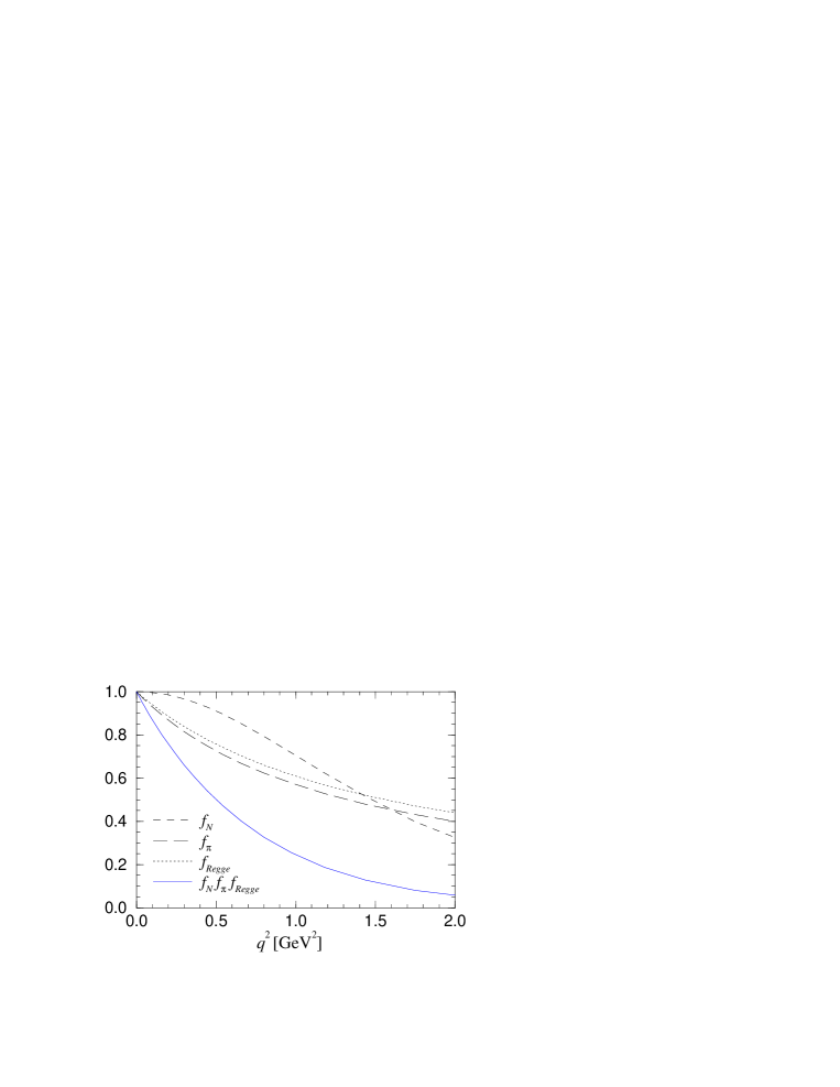
FIG. 3.: Cutoff form factors as a function of the off-shell 3-momentum squared.

FIG. 4.: Cutoff form factors as the function of the pion kinetic energy in the lab.

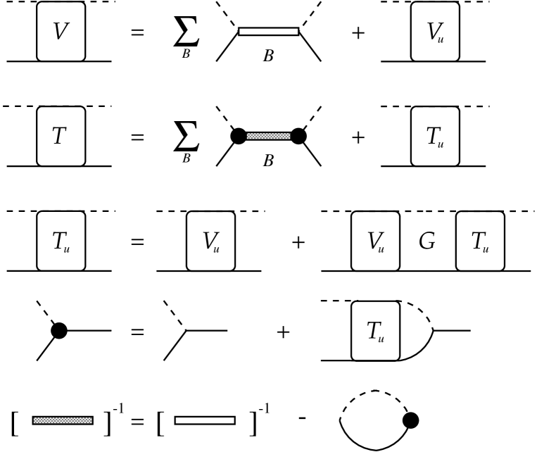
FIG. 5.: Rewriting the equation for the case when the potential can be presented as the sum of separable and non-separable potentials.

FIG. 6.: Effective range plots for the nucleon and $\rho$-meson exchange contribution. Dashed lines: $\kappa_{\rho}=0$ (Weinberg-Tomozawa contact term). Solid lines: $\kappa_{\rho}=3.7$ (vector-meson dominance). The data points are extracted from the KH80 (stars) and SM95 (dots) partial-wave analyses.

FIG. 7.: Effective range plots for the sum of the $N$, $\Delta$ and $\rho$ exchanges with $g_{\pi NN}^{2}/4\pi=13.6$, $g_{\rho}^{2}/4\pi=3$, $\kappa_{\rho}=3.7$, $f_{\pi N\Delta}^{2}/4\pi=0.36$. Dashed lines: Peccei choice; dashed-dotted lines: NEK choice; solid lines: gauge-invariant $\pi N\Delta$ coupling. Results for $S_{11}$, $S_{31}$, and $P_{33}$ waves are shown in bold lines. Data points are same as in Fig. 6.

FIG. 8.: The description of the $S$- and $P$- and $D$-wave $\pi N$ phase-shifts up to 600 MeV. Data points are from the SM95 (triangles) and KH80 (stars) partial-wave analysis. Solid lines represent the model solution. Dotted lines represent the calculation where the principal value part of the rescattering integrals is switched off (i.e., the K-matrix approximation with the same set of parameters). Dashed line for the $S_{11}$ shows the calculation when the pole contribution of the $S_{11}$ resonance is switched off.

FIG. 9.: The description of $\pi N$ phase-shifts up to 350 MeV pion lab kinetic energy. Solid lines represent the full model calculation. Legend for the data points is the same as in Fig. 8.

FIG. 10.: Description of the effective range plots for the $S$- and $P$-waves. Solid lines represent model calculation. Dotted lines are the $K$-matrix approximation with the same set parameters. Dashed-dotted line represent the full calculation with $\kappa_{\rho}=3.7$.

FIG. 11.: Fit of the $K$-matrix approximated model to $\pi N$ phase-shifts up to 350 MeV pion lab kinetic energy.

FIG. 12.: The real and imaginary parts of the self-energies

FIG. 13.: The energy dependence of the $NN^{\ast}$ mixing angle. The numbers near the curve stand for the corresponding value of the pion lab kinetic energy in GeV.

FIG. 14.: The dynamical $\pi NN$, $\pi N\Delta$ and $\pi ND_{13}$ form factors, as a function of the off-shell 3-momentum squared of the $\pi N$ state. The energy of the baryon is fixed at the $\pi N$ threshold.

FIG. 15.: The dynamical half-off-shell form factors for the case when the pion and nucleon are on-shell, as a function of the pion lab kinetic energy.

$l_{2I\,2J}$	$N\rho$ (WT)	$N\rho$ (VMD)	Peccei	NEK	$N\rho\Delta$ (WT)	$N\rho\Delta$ (VMD)	KH80 [33]	KA86 [34]	SM95 [32]
S11	0.171	0.171	0.144	0.171	0.171	0.171	0.173	0.175	0.172
S31	$-0.100$	$-0.100$	$-0.150$	$-0.100$	$-0.100$	$-0.100$	–0.101	–0.100	–0.097
P11	$-0.185$	$-0.145$	$-0.077$	$-0.076$	$-0.127$	$-0.092$	–0.081	–0.078	–0.068
P31	$-0.059$	$-0.079$	$-0.064$	$-0.085$	$-0.043$	$-0.066$	–0.045	–0.043	–0.040
P13	$-0.047$	$-0.064$	$-0.049$	$-0.069$	$-0.032$	$-0.050$	–0.030	–0.030	–0.021
P33	0.101	0.109	0.194	0.197	0.224	0.222	0.214	0.215	0.209
$\chi^{2}$	177	129	35	31	26	15	2.1	1.6	$\times$

TABLE I.: The $S$- and $P$-wave $\pi N$ scattering lengths in different models are compared to the partial-wave analyses. The $\chi^{2}$ represent the chisquare value per point with respect to the SM95 analysis (the analysis error is taken to be the same for all points and is equal to 0.005). Parameters corresponding to different calculations are given in Table II.

parameters	$N\rho$ (WT)	$N\rho$ (VMD)	Peccei	NEK	$N\rho\Delta$ (WT)	$N\rho\Delta$ (VMD)
$g_{\pi NN}^{2}/4\pi$	13.8	13.8	13.8	13.8	13.8	13.8
$g_{\rho NN}g_{\rho\pi\pi}/4\pi$	3.15	3.15	3.4	3.15	3.15	3.15
$\kappa_{\rho}$	0.0	3.7	3.7	0.0	0.0	3.7
$f_{\pi N\Delta}^{2}/4\pi$	$\times$	$\times$	0.31	0.36	0.6	0.55
$z_{\Delta}$	$\times$	$\times$	$-0.25$	0.5	$\times$	$\times$

TABLE II.: Parameters corresponding to calculations of Table I. Values in bold were varied to give a best fit of the scattering lengths.

$l_{2I\,2J}$	$N\rho\Delta\sigma$ (A)	$N\rho\Delta\sigma$ (B)	SM95 [32]
S11	0.170	0.170	0.172
S31	$-0.100$	$-0.100$	$-0.097$
P11	$-0.068$	$-0.069$	$-0.068$
P31	$-0.039$	$-0.039$	$-0.040$
P13	$-0.024$	$-0.023$	$-0.021$
P33	0.209	0.209	0.209
$\chi^{2}$	0.16	0.13	$\times$

TABLE III.: Scattering lengths resulting from the sum of $N$, $\Delta$, $\rho$, and $\sigma$ tree-level exchanges. Parameters corresponding to different models are given in Table IV.

parameters	$N\rho\Delta\sigma$ (A)	$N\rho\Delta\sigma$ (B)
$g_{\pi NN}^{2}/4\pi$	13.8	13.8
$g_{\rho NN}g_{\rho\pi\pi}/4\pi$	3.15	3.15
$\kappa_{\rho}$	0.0	4.6
$f_{\pi N\Delta}^{2}/4\pi$	0.28	0.30
$z_{\Delta}$	0.5	$\times$
$g_{\sigma NN}g_{\sigma\pi\pi}m_{N}/(8\pi m_{\pi})$	2.1	2.0
$c_{\sigma}$	1.0	1.0

TABLE IV.: Parameters corresponding to the calculation in Table III. Values in bold were established by the fit. Model A uses the conventional $\pi N\Delta$ coupling, while model B uses the “gauge-invariant” coupling.

field	coupling constants	masses [GeV]
$N$	$\frac{g_{\pi NN}^{2}}{4\pi}=13.8$ ($f_{\pi NN}^{2}$=0.0757)	$m_{N}=0.9383,\,\,{\it\Lambda}_{N}={\bf 1.8}$
$\pi$		$m_{\pi}=0.139,\,\,{\it\Lambda}_{\pi}={\bf 1.16}$
$N^{\ast}$	$\frac{g_{\pi NN^{\ast}}^{2}}{4\pi}={\bf 2.7}$	$m_{N^{\ast}}={\bf 1.438},\,\,{\it\Lambda}_{N^{\ast}}={\it\Lambda}_{N}$
$\Delta$	$\frac{f_{\pi N\Delta}^{2}}{4\pi}={\bf 0.43}$	$m_{\Delta}={\bf 1.252},\,\,{\it\Lambda}_{\Delta}={\bf 1.5}$
$D_{13}$	$\frac{f_{\pi ND}^{2}}{4\pi}={\bf 0.6}$	$m_{D}={\bf 1.525},\,\,{\it\Lambda}_{D}={\bf 1.7}$
$\rho$	$\frac{g_{\rho NN}g_{\rho\pi\pi}}{4\pi}={\bf 2.85},\,\kappa_{\rho}={\bf 1.8}$	$m_{\rho}={0.77},\,\,{\it\Lambda}_{\rho}={\bf 1.9}$
$\sigma$	$\frac{g_{\sigma NN}g_{\sigma\pi\pi}}{4\pi}\frac{m_{N}}{2m_{\pi}}={\bf 1.0},\,c_{\sigma}={\bf 0.75}$	$m_{\sigma}=0.55,\,\,{\it\Lambda}_{\sigma}={\bf 1.1}$
$S_{11}$	$\frac{f_{\pi NS_{11}}^{2}}{4\pi}={\bf 0.6}$	$m_{S_{11}}={\bf 1.555},\,\,{\it\Lambda}_{S_{11}}={\bf 2.0}$

TABLE V.: The model parameters. The values given in bold were varied during the fit.

field	coupling constants	masses [GeV]
$N$	$\frac{g_{\pi NN}^{2}}{4\pi}={13.8}$ ($f_{\pi NN}^{2}$=0.0757)	$m_{N}={0.9383},\,\,{\it\Lambda}_{N}={\bf 2.2}$
$\pi$		$m_{\pi}={0.139}$
$N^{\ast}$	$\frac{g_{\pi NN^{\ast}}^{2}}{4\pi}={\bf 2.6}$	$m_{N^{\ast}}={\bf 1.47},\,\,{\it\Lambda}_{N^{\ast}}={\it\Lambda}_{N}$
$\Delta$	$\frac{f_{\pi N\Delta}^{2}}{4\pi}={\bf 0.36}$	$m_{\Delta}={\bf 1.232},\,\,{\it\Lambda}_{\Delta}={\bf 2.6}$
$D_{13}$	$\frac{f_{\pi ND}^{2}}{4\pi}={\bf 0.8}$	$m_{D}={\bf 1.525},\,\,{\it\Lambda}_{D}={\bf 1.7}$
$\rho$	$\frac{g_{\rho NN}g_{\rho\pi\pi}}{4\pi}={\bf 3.1},\,\kappa_{\rho}={\bf 2.7}$	$m_{\rho}={0.77},\,\,{\it\Lambda}_{\rho}={\bf 1.3}$
$\sigma$	$\frac{g_{\sigma NN}g_{\sigma\pi\pi}}{4\pi}\frac{m_{N}}{2m_{\pi}}={\bf 1.3},\,c_{\sigma}={\bf 1.0}$	$m_{\sigma}=0.55,\,\,{\it\Lambda}_{\sigma}={\bf 1.9}$

TABLE VI.: The parameters of the $K$-matrix calculation, see Fig. 11.

field	$Z_{1}$	$Z_{2}$	$m_{0}$ [GeV]
$N$	0.63	0.72	1.090
$N^{\ast}$	0.63	0.95	0.960
$\Delta$	0.68	1.01	1.390
$D_{13}$	0.93	1.03	1.512
$S_{11}$	0.97	1.09	1.555

TABLE VII.: The renormalization constants obtained in the model.

REFERENCES

• [1] H. A. Bethe and F. de Hoffmann, Vol. 2, Mesons and Fields, (Peterson & Co., New York, 1956); S. L. Adler and R. F. Dashen, Current Algebra and Application to Particle Physics, (Benjamin, New York, 1968); B. H. Bransden and R. G. Moorhouse, The Pion-Nucleon System, (Princeton U.P., Princeton NJ, 1973); V. De Alfaro, S. Fubini, G. Furlan and C. Rossetti, Currents in Hadron Physics, (North-Holland, Amsterdam, 1973).
• [2] G. Höhler, in Landolt-Börnstein, New Series, Vol. I/9b, edited by H. Shopper (Springer, Berlin-Heidelberg, 1983).
• [3] B. C. Pearce and B. K. Jennings, Nucl. Phys. A528, 655 (1991).
• [4] C. C. Lee, S. N. Yang, and T.-S. H. Lee, J. Phys. G 17, 131 (1991).
• [5] F. Gross and Y. Surya, Phys. Rev. C 47, 703 (1993); 53, 2422 (1996).
• [6] C. Schültz, J. W. Durzo, K. Holinde, and J. Speth, Phys. Rev. C 49, 2671 (1994); C. Schültz, J. W. Durzo, K. Holinde, B. C. Pearce, and J. Speth, ibid. 51, 1374 (1995).
• [7] C. T. Hung, S. N. Yang, and T.-S. H. Lee, J. Phys. G 20, 1531 (1994).
• [8] T. Sato and T.-S. H. Lee, Phys. Rev. C 54, 2660 (1996).
• [9] A. D. Lahiff and I. R. Afnan, Few-Body Syst. Suppl. 10, 147 (1999); Phys. Rev. C 60, 024608 (1999).
• [10] V. Pascalutsa and J. A. Tjon, Nucl. Phys. A631, 534c (1998); Phys. Lett. B435, 245 (1998).
• [11] V. Pascalutsa and J. A. Tjon, Few-Body Syst. Suppl. 10, 105 (1999).
• [12] M. Gell-Mann and M. Lévy, Nuovo Cimento 16, 705 (1960).
• [13] S. Weinberg, Phys. Rev. Lett. 16, 169 (1966); Phys. Rev. 166, 1568 (1967).
• [14] J. Gasser, M. E. Sainio, and A. Svarć, Nucl. Phys. B307, 779 (1988); V. Bernard, N. Kaiser, and U.-G. Meissner, Int. J. Mod. Phys. E4, 193 (1995); A. Datta and S. Pakvasa, Phys. Rev. D 56, 4322 (1997); M. Mojzis, Eur. Phys. J. C2, 181 (1998); N. Fettes, U.-G. Meissner, and S. Steininger, Nucl. Phys. A640, 199 (1998); T. Becher and H. Leutwyler, Eur. Phys. J. C9, 643 (1999).
• [15] H. M. Nieland and J. A. Tjon, Phys. Lett. 27B, 309 (1968); H. M. Nieland, PhD thesis, University of Nijmegen, 1971.
• [16] F. Gross, Phys. Rev. 186, 1448 (1969); Phys. Rev. C 26, 2203 (1982).
• [17] I. T. Todorov, in Properties of the Fundamental Interactions, edited by A. Zichichi (Bologna, Compositori, 1973), Vol. 9, Part C, p. 953.
• [18] V. B. Mandelzweig and S. J. Wallace, Phys. Lett. B197, 469 (1987); S. J. Wallace and V. B. Mandelzweig, Nucl. Phys. A503, 673 (1989).
• [19] E. D. Cooper and B. K. Jennings, Nucl. Phys. A500, 553 (1989).
• [20] V. Pascalutsa and J. A. Tjon, Phys. Rev. C 60, 034005 (1999).
• [21] G. F. Chew and F. E. Low, Phys. Rev. 101, 1570 (1956).
• [22] B. D. Serot and J. D. Walecka, Int. J. Mod. Phys. E6, 515 (1997).
• [23] W. Rarita and J. Schwinger, Phys. Rev. 60, 61 (1941).
• [24] G. Velo and D. Zwanziger, Phys. Rev. 186, 267 (1969).
• [25] L. P. S. Singh, Phys. Rev. D 7, 1256 (1973).
• [26] K. Johnson and E. C. G. Sudarshan, Ann. Phys. (NY) 13, 126 (1961).
• [27] C. R. Hagen, Phys. Rev. D 4, 2204 (1971).
• [28] R. D. Peccei, Phys. Rev. 176, 1812 (1968).
• [29] L. M. Nath, B. Etemadi, and J. D. Kimel, Phys. Rev. D 3, 2153 (1971).
• [30] V. Pascalutsa, Phys. Rev. D 58, 096002 (1998).
• [31] V. Pascalutsa and R. Timmermans, Phys. Rev. C 60, 042201 (1999).
• [32] R. A. Arndt, I. Strakovsky and R. L. Workman, Phys. Rev. C 52, 2120 (1995).
• [33] R. Koch and E. Pietarinen, Nucl. Phys. A336, 331 (1980).
• [34] R. Koch, Nucl. Phys. A448, 707 (1986).
• [35] G. F. Chew, M. L. Goldberger, F. E. Low, and Y. Nambu, Phys. Rev. 106, 1337 (1957).
• [36] F. Gross, preprint JLAB-THY-99-24, nucl-th/9908084.
• [37] J. A. Tjon, in Hadronic Physics with multi-GeV Electrons, Les Houches Series (New Science Publishers, New York, 1990), p. 89.
• [38] E. Salpeter, Phys. Rev. 87, 328 (1952).
• [39] P. C. Tiemeijer and J. A. Tjon, Phys. Rev. C 48, 896 (1993); 49, 494 (1994); P. C. Tiemeijer, Ph.D. thesis, University of Utrecht, 1993.
• [40] G. Höhler and H.M. Staudenmaier, $\pi N$ Newsletter 11, 194 (1995).
• [41] S. Weinberg, Phys. Rev. Lett. 17, 616 (1966); Y. Tomozawa, Nuovo Cimento A 46, 707 (1966).
• [42] S. Weinberg, The Quantum Theory of Fields, (Cambridge U. P., Cambridge, New York, 1996), Vol. 2, Chapter 19.
• [43] K. Kawarabayashi and M. Suzuki, Phys. Rev. Lett. 16, 255 (1966); Riazuddin and Fayyazuddin, Phys. Rev. 147, 1071 (1966).
• [44] T. Feuster and U. Mosel, Phys. Rev. C 58, 457 (1998); 59, 460 (1999).
• [45] A. Yu. Korchin, O. Scholten, and R. Timmermans, Phys. Lett. B438, 1 (1998).
• [46] V. Pascalutsa, Ph.D. thesis, University of Utrecht, 1998, Section 3.5.
• [47] J. Fleischer and J. A. Tjon, Nucl. Phys. B84, 375 (1975); Phys. Rev. D 15, 2537 (1977); 21, 87 (1980).
• [48] T.-Y. Saito and I. R. Afnan, Phys. Rev. C 50, 2756 (1994); Few-Body Systems 18, 101 (1996).
• [49] C. Schültz, J. Haidenbauer, and K. Holinde, Phys. Rev. C 54, 1561 (1996).
• [50] V. Stoks, R. G. E. Timmermans, and J. J. de Swart, Phys. Rev. C 47, 512 (1993); J. J. de Swart, M. C. M. Rentmeester, and R. G. E. Timmermans, $\pi N$ Newsletter 13 (1997) 96.
• [51] M. Jacob and G. C. Wick, Ann. Phys. (NY) 7, 404 (1959).
• [52] J.J. Kubis, Phys. Rev. D 6, 547 (1972).
Refer to caption