EVENT-BY-EVENT PHYSICS IN
RELATIVISTIC HEAVY-ION COLLISIONS

Abstract

Motivated by forthcoming experiments at RHIC and LHC, and results from SPS, a review is given of the present state of event-by-event fluctuations in ultrarelativistic heavy-ion collisions. Fluctuations in particle multiplicities, ratios, transverse momenta, rapidity, etc. are calculated in participant nucleon as well as thermal models. The physical observables, including multiplicity, kaon to pion ratios, and transverse momenta agree well with recent NA49 data at the SPS, and indicate that such studies do not yet reveal the presence of new physics. Predictions for RHIC and LHC energies are given. The centrality dependence with and without a phase transition to a quark-gluon plasma is discussed - in particular, how the physical quantities are expected to display a qualitative different behavior in case of a phase transition, and can be signaled by anomalous fluctuations and correlations in a number of observables.

1 Introduction

The importance of event-by-event physics is evident from the following simple analogy: Stick a sheet of paper out of your window on a rainy day. Keeping it there for a long time - corresponding to averaging - the paper will become uniformly wet and one would conclude that rain is a uniform mist. If, however, one keeps the sheet of paper in the rain for a few seconds only, one observes the striking droplet structure of rain. Incidentally, one has also demonstrated the liquid-gas phase transition! Analyzing many events gives good statistics and may reveal rare events as snow or hail and thus other phase transitions. The statistics of droplet sizes will also tell something about the fragmentation, surface tension, etc. By varying initial conditions as timing and orienting the paper, one can further determine the speed and direction of the rain drops.

Central ultrarelativistic collisions at RHIC and LHC are expected to produce about $\sim 10^{4}$ particles, and thus present one with the remarkable opportunity to analyze, on an event-by-event basis, fluctuations in physical observables such particle multiplicities, transverse momenta, correlations and ratios. Analysis of single events with large statistics can reveal very different physics than studying averages over a large statistical sample of events. The use of Hanbury Brown–Twiss correlations to extract the system geometry is a familiar application of event-by-event physics in nuclear collisions [1] and elsewhere, e.g, in sonoluminoscence [2]. The power of this tool has been strikingly illustrated in study of interference between Bose-Einstein condensates in trapped atomic systems [3]. Fluctuations in the microwave background radiation as recently measured by COBE [4] restrict cosmological parameters for the single Big Bang event of our Universe. Large neutrons stars velocities have been measured recently [5] which indicate that the supernova collapse is very asymmetrical and leads to large event-by-event fluctuations in “kick” velocities during formation of neutron stars.

The tools applied to study these phenomena do, however, vary in order to optimize the analysis and due to limited statistics. The COBE and the interference in Bose-Einstein condensates require study of fluctuations within a single event. The HBT studies in heavy-ion collisions and sonoluminosence requires further averaging over many events in order to obtain sufficient statistics; one has not yet studied fluctuations in source radii event-by-event. Anisotropic flow requires an event-plane reconstruction in each event [6] but again averaging over many events is necessary to obtain a statistically relevant measurement of the flow. The event-by-event fluctuations in heavy-ion collisions (and neutron star kick velocities) go a step further by studying variations from event to event.

Studying event-by-event fluctuations in ultrarelativistic heavy ion collisions to extract new physics was proposed in a series of papers [7, 8, 9], in which the analysis of transverse energy fluctuations in central collisions [10] was used to extract evidence within the binary collision picture for color, or cross-section, fluctuations. More recent theoretical papers have focussed on different aspects of these fluctuations, such as searching for evidence for thermalization [11, 12, 13], correlations between transverse momentum and multiplicity [14], critical fluctuations at the QCD phase transition [15, 16, 17, 18, 19] and other correlations between collective quantities [20].

Intermittency [21] studies of factorial moments of multiplicities are related to event-by-event fluctuations. One of the motivations for intermittency studies was the idea of self-similarity on small scales, an idea borrowed from chaos theories. The factorial moments of particle multiplicities did find approximate power law behavior when the intervals of rapidity and angles were made increasingly smaller, at least until a certain small scale. The power law scaling in nucleus-nucleus collisions was, however, weaker than in proton-proton collisions. This indicated that the stronger correlations in proton-proton collisions were mainly due to resonances, minijets and other short range correlations, but that they were averaged out in nuclear collisions by summing over the many individual participating nucleons. The scaling was not a collective phenomenon and indications of new physics were not found [22]. In more recent event-by-event fluctuation studies the self-similar scaling idea is abandoned. They concentrate on the mean and the variance of the particle multiplicities per event and correlations between different particle species, transverse momentum, azimuthal angle, etc. One directly compares to expectations from proton-proton collisions scaled up by the number of participants. One follows these fluctuations and correlations for heavy-ion collisions as function of centrality and system size searching for anomalous behavior as compared to proton-proton collisions.

Recently NA49 has presented a prototypical event-by-event analysis of fluctuations in central Pb+Pb collisions at 158 GeV per nucleon at the SPS, which produce more than a thousand particles per event [11]. The analysis has been carried out on $\sim$100.000 such events measuring fluctuations in multiplicities, particle ratios, transverse momentum, etc.

Results from the RHIC collider are eagerly awaited [23]. The hope is to observe the phase transition to quark-gluon plasma, the chirally restored hadronic matter and/or deconfinement. This may be by distinct signals of enhanced rapidity and multiplicity fluctuations [24, 17] in conjunction with J/$\Psi$ suppression, strangeness enhancement, $\eta^{\prime}$ enhancement, constant (critical) temperatures vs. transverse enery or rapidity density [25], transverse flow or other collective quantities as function of centrality, transverse energy or multiplicity as will be discussed in detail below.

The purpose of this review is to understand these and other possible fluctuations. We find that the physical observables, including multiplicity, kaon to pion ratios, and transverse momenta agree well with recent NA49 data at the SPS, and indicate that such studies do not yet reveal the presence of new physics. Predictions for RHIC and LHC energies are given. The centrality dependence with and without a phase transition to a quark-gluon plasma is discussed - in particular, how the physical quantities are expected to display a qualitative different behavior in case of a phase transition, and how a first order phase transition could be signaled by very large fluctuations.

2 Phase Transitions and Fluctuations

Lattice QCD calculations find a phase transition in strongly interacting matter which is accompanied by a strong increase of the number of effective degrees of freedom [26, 27]. The Early Universe underwent this transition at a time $t=0.3-0.4(T_{c}/MeV)^{-2}$ seconds. For a hadronic gas melting temperature of $T_{c}=150$ MeV this occurred around $15$ microseconds after the Big Bang. By colliding heavy nuclei we expect to reproduce this transition at sufficiently high collisions energies.

2.1 Order of the QCD phase transition

The nature and order of the transition is not known very well. Lattice calculations can be performed for zero quark and baryon chemical potential only, $\mu_{B}=0$, where they suggest that QCD has a weak first order transition provided that the strange quark is sufficiently light [26, 27], that is for 3 or more massless quark flavors. The transition is due to chiral symmetry restoration and occur at a critical temperature $T_{C}\simeq 150$ MeV. In pure SU(3) gauge theory (that is no quarks, $N_{f}=0$) the transition is a deconfinement transition which is of first order and occurs at a higher temperature $T_{c}\simeq 260$ MeV.

However, when the strange or the up and down quark masses become massive, the QCD transition changes to a smooth cross over. The phase diagram is then like the liquid-gas phase diagram with a critical point above which the transition goes continuously through the vapor phase. For reasonable values for the strange quark mass, $m_{s}\sim 150$ MeV and small up and down quark masses, lattice calculations find either a weak first order transition [26, 27] or a smooth soft cross-over [28]. In case of a weak first order transition, the latent heat and density discontinuities and the signals, that depend on these quantities, will be small.

For exactly two massless flavors, $m_{u,d}=0$ and $m_{s}=\infty$, the transition is second order at small baryon chemical potential. Random matrix theory finds a 2nd order phase transition at high temperatures which, however, change into a 1st order transition above a certain baryon density - the tricritical point. For small up and down quark masses the transition changes to a continuous cross-over at zero baryon chemical potential but remains a first order at large baryon chemical potential. A critical point must therefore exist at small but finite baryon chemical potential which may be searched for in relativistic heavy-ion collisions [17, 18, 19].

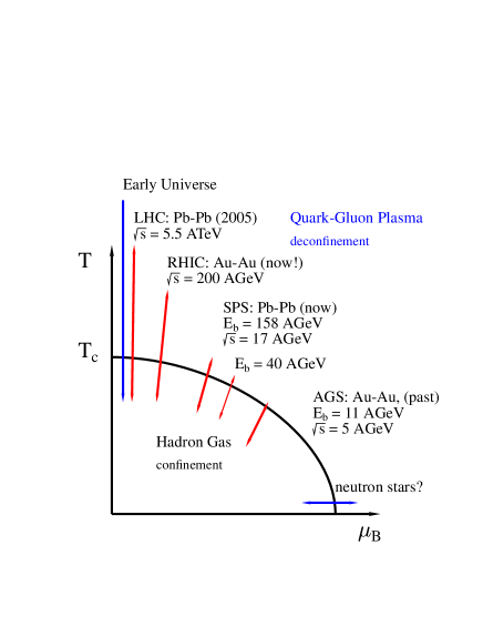
Figure 1: An illustration of the QCD phase diagram, temperature vs. baryon chemical potential. The regions of the phase diagram probed by various high energy nuclear collisions are sketched by arrows. From [29].

2.2 Density, rapidity, temperature and other fluctuations

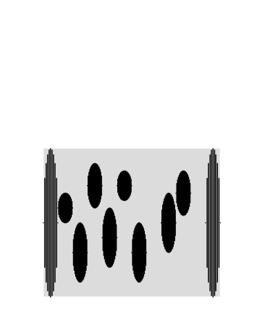
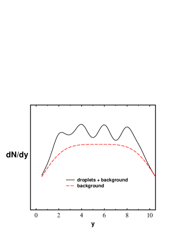
Figure 2: Sketch of droplet formation (top) in a continuous background of hadron vs. $\eta$. The corresponding rapidity distributions (bottom) are shown for the continuous hadronic background with and without droplets (target and projectile fragmentation regions are excluded).

Fluctuations are very sensitive to the nature of the transition. In case of a second order phase transition the specific heat diverges, and this has been argued to reduce the fluctuations drastically if the matter freezes out at $T_{c}$ [15, 16, 17, 18]. For example, the temperature fluctuations have a probability distribution [30]

$$w\sim\exp(-C_{V}(\frac{\Delta T}{T})^{2})\,;$$ (1)

a diverging specific heat near a 2nd order phase transition would then remove fluctuations if matter is in global thermal equilibrium. The implications of such critical phenomena near second order phase transitions and critical points are discussed in detail in [17, 18]. It is found that the expansion of the systems slows the growth of the correlation lengths associated with the critical phenomena and the systems “slows out of equilibrium”, which affects the experimental signatures related to transverse momenta and temperatures.

First order phase transitions are contrarily expected to lead to large fluctuations due to droplet formation [31] or more generally density or temperature fluctuations. These hot droplets will expand and hadronize in contrast to cold static quark matter droplets that may exist in cores of neutron stars [32]. In case of a first order phase transition relativistic heavy ion collisions lead to interesting scenarios in which matter is compressed, heated and undergoes chiral restoration. If the subsequent expansion is sufficiently rapid, matter will pass the phase coexistence curve with little effect and supercool [33, 34]. This suggests the possible formation of “droplets” of supercooled chiral symmetric matter with relatively high baryon and energy densities in a background of low density broken symmetry matter. These droplets can persist until the system reachs the spinodal line and then return rapidly to the now-unique broken symmetry minimum. A large mismatch in density and energy density seems to be a robust prediction for a first order transition at large baryon densities. At high temperatures, which is more relevant for relativistic heavy-ion collisions (see Fig. (1)), the transition is probably at most weakly first order as discussed above.

Density fluctuations may appear both for a first order phase transition and for a smooth cross-over. If the transitions is first order, matter may supercool and subsequently create fluctuations in a number of quantities. Density fluctuations in the form of hot spots or droplets of dense matter with hadronic gas in between is a likely outcome (see Fig. (2)). Even if the transition is a smooth cross-over, the resulting soft equation of state has a small sound speed, $c_{s}^{2}=\partial P/\partial\epsilon$. The equation of state $P(\epsilon)$ has in both cases a flat region that may be hard to distinguish in a finite systems existing for a short time only. We do not know the early non-equilibrium stages of relativistic nuclear collisions and the resulting initial density fluctuations, hot spots, etc. If the system becomes thermalized at some stage, then a smaller $c_{s}^{2}$ is likely to allow for larger density fluctuations since the pressure difference is smaller. Furthermore, in the subsequent expansion the density fluctuations are not equilibrated as fast when $c_{s}^{2}$ is small because the pressure differences, that drive the differential expansion, are small. The dissipation of an initial density fluctuations can be estimated by a stability analysis [35]. Linearizing the hydrodynamic equations in small fluctuations around the Bjorken scaling solution, an entropy fluctuation is typically damped by a factor (see Appendix A for details)

$$\frac{\delta S_{final}}{\delta S_{initial}}\simeq\left(\frac{\tau_{0}}{\tau_{f}}\right)^{|Re[\lambda_{\pm}]|}\,.$$ (2)

Here, a typical formation time is $\tau_{0}\simeq 1$ fm/c and freezeout time $\tau_{f}\simeq 8$ fm/c as extracted from HBT studies [1]. The eigenvalues $\lambda_{\pm}$ depend on the sound speed and the wave length of the rapidity fluctuations. As described in more detail in Appendix A, one of the eigenvalues are small and vanish for $c_{s}=0$. The resulting suppression of an initial density fluctuations during expansion is typically smaller than a factor 0.5. If density fluctuations are enhanced initially due to a softening of the equation of state due to smooth cross over, then they will largely be preserved later on. Yet, such fluctuations will be smaller than for a true first order transition forming supercooled droplets.

Let us assume that hadrons emerge from a collection of density fluctuations or droplets with a Boltzmann distribution with temperature $T$ and from a more or less continous background obeying approximate Bjorken scaling. The resulting particle distribution is

$$\frac{dN}{dyd^{2}p_{t}}\propto\sum_{i}f_{i}\,e^{-m_{t}\cosh(y-\eta_{i})/T}\,+\,{\rm background}\,.$$ (3)

Here, $y$ is the particle rapidity and $p_{t}$ its transverse momentum, $f_{i}$ is the number of particles hadronizing from each droplet i, and

$$\eta_{i}=\frac{1}{2}\log\frac{t_{i}+z_{i}}{t_{i}-z_{i}}=\frac{1}{2}\log\frac{1+v_{i}}{1-v_{i}}\,$$ (4)

is the rapidity of droplet i. The size, number and separation between droplets or density fluctuations will depend on the violent initial conditions. Between droplets a relatively continuous background of hadrons is expected in coexistence. In (3) the droplet is assumed not to expand internally neither longitudinally nor transversely. If it does expand, the emerging hadrons will have a wider distribution of rapidities which will be harder to distinguish from the background.

When $m_{t}/T\gg 1$, we can approximate $\cosh(y-\eta_{i})\simeq 1+\frac{1}{2}(y-\eta_{i})^{2}$ in Eq.(3). The Boltzmann factor determines the width of the droplet rapidity distribution as $\sim\sqrt{T/m_{t}}$. The rapidity distribution will display fluctuations in rapidity event by event when the droplets are separated by rapidities larger than $|\eta_{i}-\eta_{j}|\raisebox{-2.15277pt}{$\stackrel{{\scriptstyle>}}{{\sim}}$}\sqrt{T/m_{t}}$. If they are evenly distributed by smaller rapidity differences, the resulting rapidity distribution (3) will appear flat.

The droplets are separated in rapidity by $|\eta_{i}-\eta_{j}|\sim\Delta z/\tau_{0}$, where $\Delta z$ is the correlation length in the dense and hot mixed phase and $\tau_{0}$ is the invariant time after collision at which the droplets form. Assuming that $\Delta z\sim 1$fm — a typical hadronic scale — and that the droplets form very early $\tau_{0}\raisebox{-2.15277pt}{$\stackrel{{\scriptstyle<}}{{\sim}}$}1$fm/c, we find that indeed $|\eta_{i}-\eta_{j}|\raisebox{-2.15277pt}{$\stackrel{{\scriptstyle>}}{{\sim}}$}\sqrt{T/m_{t}}$ even for the light pions. If strong transverse flow is present in the source, the droplets may also move in a transverse direction. In that case the distribution in $p_{t}$ may be non-thermal and azimuthally asymmetric.

Even if the transition is not first order, fluctuations may still occur in the matter that undergoes a transition. The fluctuations may be in density, chiral symmetry [36], strangeness, or other quantities and show up in the associated particle multiplicities. The “anomalous” fluctuations depend not only on the type and order of the transition, but also on the speed by which the collision zone goes through the transition, the degree of equilibrium, the subsequent hadronization process, the amount of rescatterings between hadronization and freezeout, etc. It may be that any sign of the transition is smeared out and erased before freezeout. That no anomalous event-by-event fluctuations have been found at CERN [24] within experimental accuracy indicate that no transition took place or that the signals were erased before freezeout. Whether they remain at RHIC is yet to be discovered and we shall provide some tools for the analysis in the following sections.

3 Multiplicity Fluctuations in Relativistic Heavy-Ion Collisions

Figure 3: Charged particle density per participant at midrapidity are shown vs. c.m. energy for $pp$ and $\bar{p}p$ data [39, 40, 41] with open symbols. Full curve presents a linear fit to $pp$ and $\bar{p}p$ data up to RHIC energies. Pb+Pb data from NA49 [11] and Au+Au data from PHOBOS [23] per participant are shown with filled symbols, and exceed the $pp$ and ${\bar{p}}p$ by ca. 30% (dashed curve).

In order to be able to extract new physics associated with fluctuations, it is necessary to understand the role of expected statistical fluctuations. Our aim here is to study the sources of these fluctuations in collisions. As we shall see, the current NA49 data (see Fig. (6)) can be essentially understood on the basis of straightforward statistical arguments. Expected sources of fluctuations include impact parameter fluctuations, fluctuations in the number of primary collisions and in the results of such collisions, fluctuations in the relative orientation during the collision of deformed nuclei [10], effects of rescattering of secondaries, and QCD color fluctuations. Since fluctuations in collisions are sensitive to the amount of rescattering of secondaries taking place, we discuss in detail two limiting cases, the participant or “wounded nucleon model” (WNM) [37], in which one assumes that particle production occurs in the individual participant nucleons and rescattering of secondaries is ignored, and the thermal limit in which scatterings bring the system into local thermal equilibrium.

Data at AGS, SPS and RHIC energies show that multiplicities are enhanced by $\sim$30% in central collisions between heavy ($A\simeq 200$) nuclei as compared to the WNM prediction (see Fig. (3)). Whether rescatterings increase relative fluctuations through greater production of multiplicity, transverse momenta, etc., or decrease fluctuations by involving a greater number of degrees of freedom, is not immediately obvious [7, 8]. Rescatterings probably increase both the average multiplicity and its variance but whether the relative amount of fluctuations are increased is model dependent. It has even been found in relativistic heavy ion collisions that the multiplicity fluctuations increase in the first few rescattering but then decrease again as the thermal limit is approached. VENUS simulations [38] showed that rescattering had negligible effects on transverse energy fluctuations.

We first review known multiplicities and fluctuations in the basic $pp$ collisions, go on to study nucleus-nucleus collisions, and finally show in a simple model how phase transitions are capable of producing very significant fluctuations in particle multiplicities.

3.1 Charged particle production in $pp$ and $p\bar{p}$ reactions

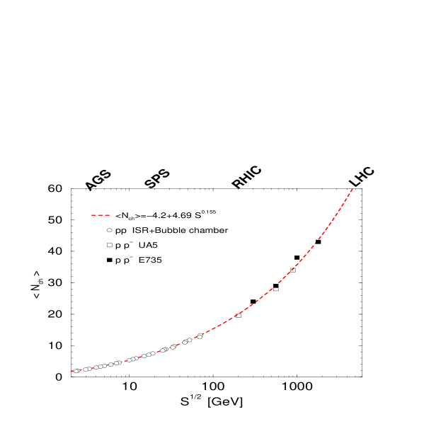
Figure 4: The total number of charged particles produced in $pp$ and $p\bar{p}$ collisions vs. cms energy $s^{1/2}$. Data from bubble chamber [40], ISR [42], UA5 [41] and FNAL E735 [43].

Participant models or WNMs are basically a superposition of NN collisions. Such models have been studied extensively at these energies within the last decades at several particle accelerators and we here give a brief compilation of relevant results.

The average number of charged particles produced in high energy $pp$ and ultrarelativistic $p\bar{p}$ collisions can be parametrized by

$$\langle{N_{ch}}\rangle\simeq-4.2\,+\,4.69\left(\frac{s}{{\rm GeV}^{2}}\right)^{0.155}\,,$$ (5)

for cms energies $\sqrt{s}\raisebox{-2.15277pt}{$\stackrel{{\scriptstyle>}}{{\sim}}$}2$ GeV. At ultrarelativistic energies the charged particle production is very similar in $pp$, $pn$ and $p\bar{p}$ collisions and the parametrization of Eq. (5) applies in a wide range of cms energies 2 GeV$\raisebox{-2.15277pt}{$\stackrel{{\scriptstyle<}}{{\sim}}$}s^{1/2}\raisebox{-2.15277pt}{$\stackrel{{\scriptstyle<}}{{\sim}}$}$ 2 TeV as shown in Fig. (4). At SPS, RHIC and LHC energies, $\sqrt{s}\simeq 20$, 200, 5000 GeV, we find $\langle{N_{ch}}\rangle\simeq 7.3,20,60$, respectively.

At high energies KNO scaling [44] is a good approximation. KNO scaling implies that multiplicity distributions are invariant when scaled with the average multiplicity. Thus all moments scale like

$$\langle{N_{ch}^{q}}\rangle\simeq c_{q}\langle{N_{ch}}\rangle^{q}\,,$$ (6)

at high energies where $c_{q}$ are constants independent of collision energy. The fluctuations,

$$\omega_{N}\equiv(\langle{N^{2}}\rangle-\langle{N}\rangle^{2})/\langle{N}\rangle\,,$$ (7)

therefore scale with average multiplicity, $\langle{N}\rangle$, and therefore increase with collision energy as in Eq. (5). The fluctuations in the charged particle multiplicity can be parametrized rather accurately by

$$\omega_{N_{ch}}\simeq 0.35\frac{(\langle{N_{ch}}\rangle-1)^{2}}{\langle{N_{ch}}\rangle}$$ (8)

as shown in Fig. (5) for $pp$ and $p\bar{p}$ collisions in the same wide range of energies. At the very high energies breakdown of KNO scaling has been observed in the direction that the fluctuations are slightly larger. At SPS, RHIC and LHC energies we find $\omega_{N_{ch}}\simeq 2.0,6.2,20$, respectively in $pp$ and $p\bar{p}$ collisions.

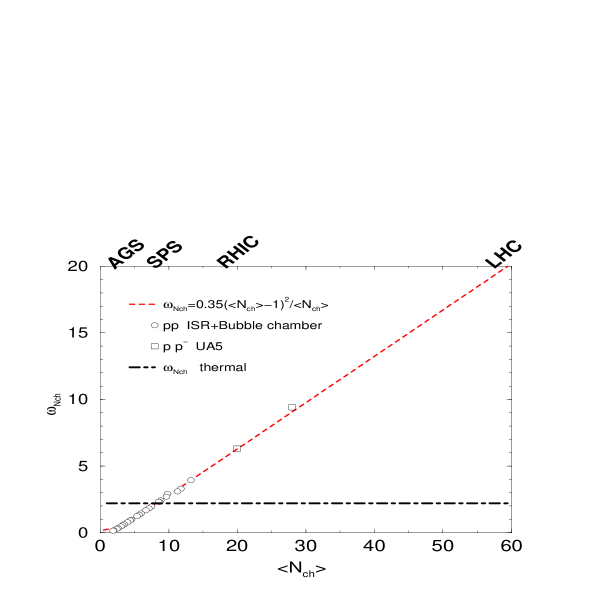
Figure 5: The fluctuations in the total number of charged particles produced in $pp$ and $p\bar{p}$ collisions from bubble chamber experiments [40], ISR [42], and UA5 [41]. Note the large difference between pp and thermal fluctuations $\omega^{th}_{N_{ch}}\simeq 2.2$ at very high energies and the “accidental” crossing with $pp$ fluctuations around SPS energies.

In nuclear (AA) collisions the number of participating nucleons $N_{p}$ grow with centrality and nuclear mass number $A$. Therefore the average charged particle multiplicity and variance grows with $N_{p}$, whereas the ratio and therefore the fluctuation $\omega_{N_{ch}}$ is independent of $N_{p}$, and equal to the fluctuations in pp collisions. (Other fluctuations such as impact parameter will be included below.) Higher moments of the multiplicity distributions are large in high energy pp and $p\bar{p}$ collisions due to KNO scaling but in nuclear collisions such higher moments are suppressed by factors of $1/N_{p}$ and are therefore less interesting than the second moment. This justifies our detailed analyzes of the variance (or rms width) of the fluctuations.

3.2 Fluctuations in the participant model

In the participant or wounded nucleon models nucleus-nucleus collisions at high energies are just a superposition of nucleon-nucleon (NN) interactions. In peripheral collisions there are only few NN collisions, the collision zone is small, rescatterings few and the WNM should therefore apply. For central nuclear collisions, however, multiple NN scatterings, energy degradation, rescatterings between produced particles and other effects complicate the particle production and do enhance the multiplicities by ca. 30% as seen in experiment (see Fig. (3)). Thermal models may better describe central collisions as will be investigated afterwards. Yet, the WNM provides a simple baseline to compare to, when going from peripheral towards central collisions.

Let us first calculate fluctuations in the participant model. Although the multiplicities are somewhat underestimated, the measured multiplicity and transverse energy in nuclear collisions at AGS and SPS energies are known to scale approximately linearly with the number of participants [45, 11]. In this picture

$$N=\sum_{i}^{N_{p}}n_{i},$$ (9)

where $N_{p}$ is the number of participants and $n_{i}$ is the number of particles produced in the acceptance by participant $i$. In the absence of correlations between $N_{p}$ and $n$, the average multiplicity is $\langle{N}\rangle=\langle{N_{p}}\rangle\langle{n}\rangle$. For example, NA49 measures charged particles in the rapidity region $4<y<5.5$ and finds $\langle{N}\rangle\simeq 270$ for central Pb+Pb collisions. Finite impact parameters $(b\raisebox{-2.15277pt}{$\stackrel{{\scriptstyle<}}{{\sim}}$}3.5$ fm) as well as surface diffuseness reduce the number of participants from the total number of nucleons $2A$ to $\langle{N_{p}}\rangle\simeq 350$ estimated from Glauber theory; thus $\langle{n}\rangle\simeq 0.77$. Squaring Eq. (9) and again assuming no correlations between different wounded nucleon emission, $\langle{n_{i}n_{j}}\rangle=\langle{n_{i}}\rangle\langle{n_{j}}\rangle$ for $i\neq j$, we find the multiplicity fluctuations (see Appendix B)

$$\omega_{N}=\omega_{n}+\langle{n}\rangle\omega_{N_{p}},$$ (10)

where $\omega_{N}$, $\omega_{n}$ and $\omega_{N_{p}}$ are the multiplicity fluctuations in the total number of particles (within the acceptance), in each source, and in the number of sources respectively.

A major source of multiplicity fluctuations per participant, $\omega_{n}$, is the limited acceptance. While each participant produces $\nu$ charged particles, only a smaller fraction $f=\langle{n}\rangle/\langle{\nu}\rangle$ are accepted. Without carrying out a detailed analysis of the acceptance, one can make a simple statistical estimate assuming that the particles are accepted randomly, in which case $n$ is binomially distributed with $\sigma(n)=\nu f(1-f)$ for fixed $\nu$. Including fluctuations in $\nu$ we obtain, similarly to Eq. (10),

$$\omega_{n}=1-f+f\omega_{\nu}\,.$$ (11)

In nucleon-nucleon collisions at SPS energies, the charged particle multiplicity is $\sim 7.3$ and $\omega_{\nu}\simeq 1.9$ [46]; as the multiplicity should be divided between the two colliding nucleons, we obtain $\langle{\nu}\rangle\simeq 3.7$ and thus $f=\langle{n}\rangle/\langle{\nu}\rangle=0.21$ for the NA49 acceptance. Consequently, we find from Eq. (11) that $\omega_{n}\simeq 1.2$. The random acceptance assumption can be improved by correcting for known rapidity correlations in charged particle production in $pp$ collisions [42, 40].

Multiplicities generally increase with centrality of the collision. We will use the term centrality as impact parameter $b$ in the collision. It is not a directly measurable quantity but is closely correlated to the transverse energy produced $E_{T}$, the measured energy in the zero degree calorimeter and the total particle multiplicity $N$ measured in some large rapidity interval. The latter is within the WNM approximately proportional to the number of participating nucleons

$$N_{p}({\bf b})=\int_{overlap}\left[\rho({\bf r}+\frac{\bf b}{2})+\rho({\bf r}-\frac{\bf b}{2})\right]d^{3}r\,.$$ (12)

For sharp sphere nuclei the number of participants drops from $N_{p}(b=0)=2A$ in central collisions to $N_{p}(b=2R)=0$ in grazing collisions. For realistic nuclei with diffuse surface and with collision probabilities given by Glauber theory, the number of participants are 5-10% smaller in central collisions but slightly larger in peripheral collisions.

As a consequence of nuclear correlations, which strongly reduce density fluctuations in the colliding nuclei, the fluctuations $\omega_{N_{p}(b)}$ in $N_{p}$ are very small for fixed impact parameter $b$ [9]. Almost all nucleons in the nuclear overlap volume collide and participate. [By contrast, the fluctuations in the number of binary collisions are non-negligible.] Cross section fluctuations play a small role in the WNM [9]. Fluctuations in the number of participants can arise when the target nucleus is deformed, since the orientations of the deformation axes vary from event to event [47]. The fluctuations, $\omega_{N_{p}}$, in the number of participants are dominated by the varying impact parameters selected by the experiment. In the NA49 experiment, for example, the zero degree calorimeter selects the 5% most central collisions, corresponding to impact parameters smaller than a centrality cut on impact parameter, $b_{c}\simeq 3.5$ fm. We have

$$\omega_{N_{p}}\langle{N_{p}}\rangle=\frac{1}{\pi b_{c}^{2}}\int_{0}^{b_{c}}d^{2}bN_{p}(b)^{2}-\langle{N_{p}}\rangle^{2}\,,$$ (13)

where $\langle{N_{p}}\rangle=(1/\pi b_{c}^{2})\int_{0}^{b_{c}}d^{2}bN_{p}(b)$. The number of participants for a given centrality, calculated in [48], can be approximated by $N_{p}(b)\simeq N_{p}(0)(1-b/2R)$ for $0\leq b\raisebox{-2.15277pt}{$\stackrel{{\scriptstyle<}}{{\sim}}$}3.5$ fm; thus

$$\omega_{N_{p}}=\frac{N_{p}(0)}{18}\left(\frac{b_{c}}{2R}\right)^{2}\,.$$ (14)

For NA49 Pb+Pb collisions with $N_{p}(0)\simeq 400$ and $(b_{c}/2R)^{2}\simeq 5\%$ we find $\omega_{N_{p}}\simeq 1.1$. Impact parameter fluctuations are thus important even for the centrality trigger of NA49. Varying the centrality cut or $b_{c}$ to control such impact parameter fluctuations (14) should enable one to extract better any more interesting intrinsic fluctuations. Recent WA98 analyzes confirm that fluctuations in photons and pions grow approximately linearly with the centrality cut $(b_{c}/2R)^{2}$ [49] as predicted by Eq. (14). The impact parameter fluctuations associated with the range of the centrality cut, such at total transverse energy or multiplicity, can therefore be removed. However, fluctuations in impact parameter may still remain for a given centrality. The Gaussian multiplicity distribution found in central collisions changes for minimum bias to a plateau-like distribution [10].

Calculating $\omega_{N}$ for the NA49 parameters, we find from Eq. (10), $\omega_{N}\simeq 1.2+(0.77)(1.1)=2.0$, in good agreement with experiment, which measures a multiplicity distribution $\propto\exp[-(N-\langle{N}\rangle)^{2}/2\langle{N}\rangle\omega_{N}^{exp}]$, where $\omega_{N}^{exp}$ is $2.01$ [11] (see Fig. (6)).

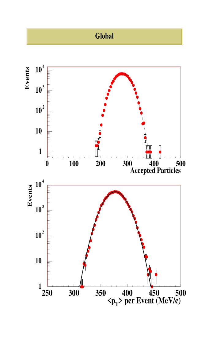
Figure 6: Event-by-event fluctuations of multiplicity (top) and $p_{t}$ (bottom) measured by NA49 in central Pb+Pb collisions at the SPS [11].

3.3 Fluctuations in the thermal model

Let us now consider, in the opposite limit of strong rescattering, fluctuations in thermal models. In a gas in equilibrium, the mean number of particles per bosonic mode $n_{a}$ is given by

$$\langle n_{a}\rangle=\left(\exp{(E_{a}/T)}-1\right)^{-1}\,,$$ (15)

with fluctuations

$$\omega_{n_{a}}=1+\langle n_{a}\rangle\,.$$ (16)

The total fluctuation in the multiplicity, $N=\sum_{a}n_{a}$, is

$$\omega^{BE}_{N}=1+\sum_{a}\langle n_{a}\rangle^{2}/\sum_{a}\langle n_{a}\rangle.$$ (17)

If the modes are taken to be momentum states, bosons/fermions have thermal fluctuations, $\omega_{N}=1\pm\langle{n_{p}^{2}}\rangle/\langle{n_{p}}\rangle$ where $n_{p}=(\exp(\epsilon_{p}/T)\mp 1)^{-1}$ is the boson/fermion distribution function, which are slightly larger/smaller than those of Poisson statistics for a Boltzmann distribution, $\omega_{N}=1$. The resulting fluctuations are $\omega^{BE}_{N}=\zeta(2)/\zeta(3)=1.37$ for massless bosons as, e.g., gluons. Massive bosons have smaller fluctuations with, for example, $\omega_{\pi}=1.11$ [50] and $\omega_{\rho}=1.01$ when $T=m_{\pi}$. Massless fermions, e.g. quarks, have $\omega_{F}=2\zeta(2)/3\zeta(3)\simeq 0.91$ independent of temperature.

Resonances are implicitly included in the WNM fluctuations. In the thermal limit resonances are found to increase total multiplicity fluctuations [17, 24] but decrease, e.g., net charged particle fluctuations [51, 52, 53, 54]. In high energy nuclear collisions, resonance decays such as $\rho\to 2\pi$, $\omega\to 3\pi$, etc., lead to half or more of the pion multiplicity. Only a small fraction $r\simeq 20-30$% produce two charged particles in a thermal hadron gas [55, 51] or in RQMD [56] (see also [57]). Not all of the decay particles from the same resonance always fall into the NA49 acceptance, $4<y<5.5$, and the fraction of pairs will be smaller; we estimate $r\simeq 0.1$. Including such resonance fluctuations in the BE fluctuations gives, similarly to Eq. (10),

$$\omega^{BE+R}_{N}=r\frac{1-r}{1+r}+(1+r)\omega_{N}^{BE}\,.$$ (18)

With $r\simeq 0.1$ we obtain $\omega^{BE+R}_{N}\simeq 1.3$. In [17] the estimated effect of resonances is about twice ours: $\omega_{N}\simeq 1.5$, not including impact parameter fluctuations.

Fluctuations in the effective collision volume add a further term $\langle{N}\rangle\sigma(V)/\langle{V}\rangle^{2}$ to $\omega^{BE+R}_{N}$. Assuming that the volume scales with the number of participants, $\omega_{V}/\langle{V}\rangle\simeq\omega_{N_{p}}/\langle{N_{p}}\rangle$, we find from Eq. (10) that $\omega_{N}=\omega^{BE+R}_{N}+\langle{n}\rangle\omega_{N_{p}}\simeq 2.1$, again consistent with the NA49 data. Because of the similarity between the magnitudes of the thermal and WNM multiplicity fluctuations, the present measurements cannot distinguish between these two limiting pictures.

3.4 Centrality dependence and degree of thermalization

It is very unfortunate that the WNM and thermal models predict the same multiplicity fluctuations in the NA49 acceptance - and that they agree with the experiment. If the numbers from the two models had been different and the experimental number in between these two, then one would have had quantified the degree of thermalization in relativistic heavy ion collisions.

The similarity of the fluctuation in the thermal and WNM is, however, a coincidence at SPS energies. As seen from Fig. (5) the fluctuations in $pp$ collisions increase with collision energy and just happen to cross the thermal fluctuations, $\omega_{thermal}\simeq 2.2$, at SPS energies.

At RHIC or LHC energies the situation will be much clearer. Here the charged particle fluctuations in $pp$ collisions are much larger as seen in Fig. (5), namely $\omega^{pp}_{N_{ch}}=6.5$, 20 at RHIC and LHC energies respectively. The thermal fluctuations remain as $\omega_{thermal}\simeq 2.2$. Therefore a dramatic reduction in event-by-event fluctuations are expected at higher energies at the nuclear collisions become more central as shown in Fig. (7).

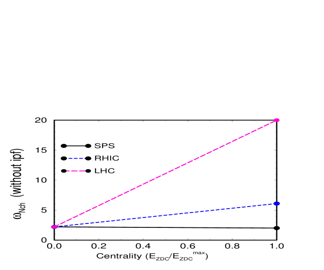
Figure 7: The fluctuation in the total number of charged particles (excluding volume fluctuations) vs. centrality or energy in the zero degree calorimeter; left are central and right are peripheral nuclear collisions. The curves are linear extrapolations between the thermal fluctuations, $\omega_{thermal}\simeq 2.2$, in central collisions to $pp$ fluctuations at SPS, RHIC, and LHC energies, $\omega^{pp}$, expected in peripheral collisions within the WNM (see text).

This can be exploited to define a “Degree of thermalization” as the measured fluctuations at a given centrality relative to those in the thermal and $pp$ limits

$${\rm Degree\,of\,thermalization}\equiv\frac{\omega_{N}^{WNM}-\omega_{N}^{exp}}{\omega_{N}^{WNM}-\omega_{N}^{thermal}}\,,$$ (19)

which ranges from unity in the thermal limit to zero in the WNM. Whereas both $\omega_{N}^{WNM}$ and $\omega_{N}^{exp}$ may depend on the acceptance the degree of thermalization Eq. (19) should not. Contributions from volume or impact parameter fluctuations may, however, be centrality dependent and should therefore be subtracted. Alternatively, the fluctuations in a ratio, e.g. $N_{-}/N_{+}$, should be taken for limited acceptances.

At RHIC and LHC it should be straight forward to measure the degree of thermalization as function of centrality. This is interesting on its own and a necessary requirement for studies of anomalous fluctuations from a phase transition.

3.5 Enhanced fluctuations in first order phase transitions

First order phase transitions can lead to rather large fluctuations in physical quantities. Thus, detection of enhanced fluctuations, beyond the elementary statistical ones considered to this point, could signal the presence of such a transition. For example, before it became clear that the chiral symmetry restoring phase transition in hot QCD is not a strong first order phase transition, it was suggested that matter undergoing a transition from chirally symmetric to broken chiral symmetry could, when expanding, supercool and form droplets, resulting in large multiplicity versus rapidity fluctuations [34]. Let us imagine that $N_{D}$ droplets fall into the acceptance, each producing $n$ particles, i.e., $\langle{N}\rangle=\langle{N_{D}}\rangle\langle{n}\rangle$. The corresponding multiplicity fluctuation is (see Appendix B)

$$\omega_{N}=\omega_{n}+\langle{n}\rangle\omega_{N_{D}}\,.$$ (20)

As in Eq. (11), we expect $\omega_{n}\sim 1$. However, unlike the case of participant fluctuations, the second term in (20) can lead to huge multiplicity fluctuations when only a few droplets fall into the acceptance; in such a case, $\langle{n}\rangle$ is large and $\omega_{N_{D}}$ of order unity. The fluctuations from droplets depends on the total number of droplets, the spread in rapidity of particles from a droplet, $\delta y\sim\sqrt{T/m_{t}}$, as well as the experimental acceptance in rapidity, $\Delta y$. When $\delta y\ll\Delta y$ and the droplets are binomially distributed in rapidity, $\omega_{N_{D}}\simeq 1-\Delta y/y_{\rm tot}$, which can be a significant fraction of unity.

In the extreme case where none or only one droplet falls into the acceptance with equal probability, we have $\omega_{N_{D}}=1/2$ and $\langle{n}\rangle=2\langle{N}\rangle$. The resulting fluctuation is $\omega_{N}\simeq\langle{N}\rangle$, which is more than two orders of magnitude larger than the expected value of order unity as currently measured in NA49. It should be said immediately that a much smaller enhancement is realistic as the transition probably is at most weakly first order and many effects will smear the signal. Yet, this simple example clearly demonstrates the importance of event-by-event fluctuations accompanying phase transitions, and illustrates how monitoring such fluctuations versus centrality becomes a promising signal, in the upcoming RHIC experiments, for the onset of a transition. It is the hope and expectation that the higher RHIC energies probe deeper into the QGP phase by creating higher temperatures and energy densities whereby larger regions of QGP are produced. The larger event multiplicities should make it possible to improve on statistics and thereby also the ability to detect anomalous fluctuations. The potential for large fluctuations (orders of magnitude) from a transition makes it worth looking for at RHIC considering the relative simplicity and accuracy (percents) of multiplicity measurements.

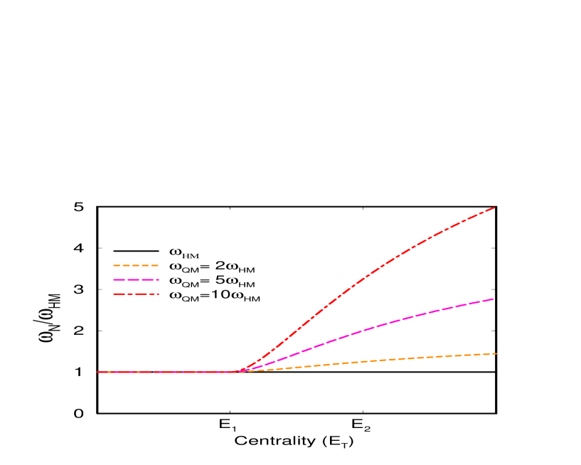
Figure 8: Qualitative picture of multiplictity fluctuations vs. centrality (total multiplicity or $E_{T}$). Anomalous fluctuations appear when a transition to a new state of matter (QM) starts at centrality $E_{1}$ (see text). Curves for different ratios of the fluctuations characterizing the two states of matter are shown.

Let us subsequently consider a less extreme model in which a transition leads to enhanced fluctuations of some kind. Assume that the total multiplicity within the acceptance arises from a normal hadronic background component ($N_{HG}$) and from a second component ($N_{QGP}$) that has undergone a transition:

$$N=N_{HG}+N_{QGP}\,.$$ (21)

Its average is $\langle{N}\rangle=\langle{N_{HG}}\rangle+\langle{N_{QGP}}\rangle$. Assuming that the multiplicity of each of these components is statistically independent, the multiplicity fluctuation becomes

$$\omega_{N}=\omega_{HG}+(\omega_{QGP}-\omega_{HG})\frac{\langle{N_{QGP}}\rangle}{\langle{N}\rangle}\,.$$ (22)

Here, $\omega_{HG}$ is the standard fluctuation in hadronic matter $\omega_{HG}\simeq 1$. The fluctuations due to the component that had experienced a phase transition, $\omega_{QGP}$, depend on the type and order of the transition, the speed with which the collision zone goes through the transition, the degree of equilibrium, the subsequent hadronization process, the number of rescatterings between hadronization and freezeout, etc. If thermal and chemical equilibration eliminate all signs of the transition, then $\omega_{QGP}\simeq\omega_{HG}$.

The amount of QM and thus $\langle{N_{QM}}\rangle$ depends on centrality, energy and nuclear masses in the collision. For a given centrality the densities vary from zero at the periphery of the collision zone to a maximum value at the center. Furthermore, the more central the collision the higher energy densities are created. The transverse energy, $E_{T}$, the total multiplicity and/or the energy in the zero-degree calorimeter, $E_{ZDC}$, have been found to be good measures of the centrality of the collision at SPS energies. Therefore, it would be very interesting to study fluctuations vs. centrality which are proportional to energy density. By varying the binning size for centrality one can also remove impact parameter fluctuations as discussed above.

If the energy density in the center of the collision zone exceeds the critical energy density for forming QM at a certain centrality, $E_{1}$, then a mixed phase of QM and HM is formed. At a higher energy density, where the critical energy density plus the latent heat for the transition is exceeded, which we shall assume occur at a centrality $E_{2}$, then a pure QM phase is produced in the center. These quantities will depend on the amount of stopping at a given centrality, the geometry, $T_{c}$, etc. In the mixed phase $E_{1}\leq E_{T}<E_{2}$, the relative amount of QM, $\langle{N_{QM}}\rangle/\langle{N}\rangle$, is proportional to both the volume of the mixed phase. and the fraction of the volume that is in the QM phase. The latter varies in the volume such that it vanishes at HM/QM boundary.

In Fig. (8) a schematic plot of the fluctuations of Eq. (22) is shown as function of centrality for various $\omega_{QM}$. Up to centrality $E_{1}$ the fluctuations are unchanged. Above the central overlap zone undergoes the transition to the QM/HM mixed phase and fluctuations start to grow when $\omega_{QM}>\omega_{HM}$. At the higher centrality, $E_{2}$ the central overlap zone is in the pure QM phase but the maximum fluctuations $\omega_{QM}$ are not reached because the surface regions of the collision zone is still in the HM phase. On the other hand, if the hadronization of the QM state is smooth and does not lead to enhanced fluctuations (i.e. if $\omega_{QGP}=\omega_{HG}$), it cannot be observed in such a study.

The multiplicity fluctuations can be studied for any kind of particles, total or ratios. Total multiplicities describe total multiplicities whereas, e.g. the ratio $\pi^{0}/(\pi^{+}+\pi^{-})$ can reveal fluctuations in chiral symmetry. The onset and magnitude of such fluctuations would reveal the symmetry and other properties of the new phase.

4 Correlations between total and net charge, baryon number or strangeness

By a combined analysis of fluctuations in, e.g., positive, negative, total and net charge as well as ratios, the intrinsic and other fluctuations as well as correlations can be extracted and exploited to reveal interesting physics as will be demonstrated in the following.

4.1 General analysis of fluctuations and correlations

Multiplicity fluctuations between various kinds of particles can be strongly correlated. As a first example, consider the multiplicities of positive and negative pions, $N_{+}$ and $N_{-}$, in a rapidity interval $\Delta y$ for any relativistic heavy-ion experiment. Similar analyzes can be performed for any two kinds of distinguishable particles.

The net positive charge from the protons in the colliding nuclei is much smaller than the total charge produced in an ultrarelativistic heavy-ion collision. For example, $\langle{N_{+}}\rangle$ exceeds $\langle{N_{-}}\rangle$ by only $\sim 15$% at in Pb$+$Pb collisions at SPS energies. The fluctuations in the number of positive and negative (or neutral) pions are also very similar, $\omega_{N_{+}}\simeq\omega_{N_{-}}$. Charged particle fluctuations have been estimated in thermal as well as participant nucleon models [24] including effects of resonances, acceptance, and impact parameter fluctuations. By varying the acceptance and centrality, the degree of thermalization can actually be determined empirically. Detailed analysis indicates that the fluctuations in central Pb+Pb collisions at the SPS are thermal whereas peripheral collisions are a superposition of pp fluctuations [64].

The fluctuations in the total ($N_{ch}=N_{+}+N_{-}$) and net ($Q=N_{+}-N_{-}$) charge are defined as [54]

$$\frac{\langle{(N_{+}\pm N_{-})^{2}}\rangle-\langle{N_{+}\pm N_{-}}\rangle^{2}}{\langle{N_{+}+N_{-}}\rangle}=$$

$$\quad\frac{\langle{N_{+}}\rangle}{\langle{N_{ch}}\rangle}\omega_{N_{+}}+\frac{\langle{N_{-}}\rangle}{\langle{N_{ch}}\rangle}\omega_{N_{-}}\,\pm\,C\,,$$ (23)

where the correlation is given by

$$C=\frac{\langle{N_{+}N_{-}}\rangle-\langle{N_{+}}\rangle\langle{N_{-}}\rangle}{\langle{N_{ch}}\rangle/2}\,.$$ (24)

Fluctuations in positive, negative, total and net charge can be combined to yield both the intrinsic fluctuations in the numbers of $N_{\pm}$ and the correlations in their production as well as a consistency check. These quantities can change as a consequence of thermalization and a possible phase transition.

In practice, $\omega_{N_{+}}\approx\omega_{N_{-}}$, so that the fluctuation in total charge simplifies to

$$\omega_{N_{ch}} \equiv \frac{\langle{N_{ch}^{2}}\rangle-\langle{N_{ch}}\rangle^{2}}{\langle{N_{ch}}\rangle}=\omega_{N_{+}}+C\,,$$ (25)

and that for the net charge becomes

$$\omega_{Q} \equiv \frac{\langle{Q^{2}}\rangle-\langle{Q}\rangle^{2}}{\langle{N_{ch}}\rangle}=\omega_{N_{+}}-C\,.$$ (26)

The fluctuation in net charge can be related to the fluctuation in the ratio of positive to negative particles

$$\omega_{Q}\simeq\langle{N_{+}/N_{-}}\rangle\langle{N_{ch}}\rangle\omega_{N_{-}/N_{+}}/4\,,$$ (27)

plus volume (or impact parameter) fluctuations [51, 53]. The virtue of this expression is that volume fluctuations can in principle be extracted empirically. Alternatively one can vary the centrality bin size or the acceptance. Furthermore, the volume fluctuations for net and total charge are proportional to the net ($\langle{N_{+}-N_{-}}\rangle$) and total ($\langle{N_{+}+N_{-}}\rangle$) charge respectively with the same prefactor. In the following we shall assume that such “trivial” volume fluctuations have been removed.

The analysis has so far been general and Eqs. (23-26) apply to any kind of distinguishable particles, e.g. positive and negative particles, pions, kaons, baryons, etc. - irrespective of what phase the system may be in, or whether it is thermal or not. In the following, we shall consider thermal equilibrium, which seems to apply to central collisions between relativistic nuclei, in order to reveal possible effects on fluctuations of the presence of a quark-gluon plasma.

4.2 Charge fluctuations in a thermal hadron gas

In a thermal hadron gas (HG) as created in relativistic in nuclear collisions, pions can be produced either directly or through the decay of heavier resonances, $\rho,\ \omega,...$. The resulting fluctuation in the measured number of pions is

$$\omega_{N_{+}}=\omega_{N_{-}}=f_{\pi}\omega_{\pi}+f_{\rho}\omega_{\rho}+f_{\omega}\omega_{\omega}+....\,,$$ (28)

where $f_{r}$ is the fraction of measured pions produced from the decay of resonance $r$, and $\sum_{r}f_{r}=1$. These mechanisms are assumed to be independent, which is valid in a thermal system.

The heavier resonances such as $\rho^{0},\omega,...$ decay into pairs of $\pi^{+}\pi^{-}$ and thus lead to a correlation

$$C^{HG}=\frac{1}{3}f_{\rho}+f_{\omega}+....\,.$$ (29)

Resonances reduce the fluctuations in net charge in a HG in chemical equilibrium at temperature $T=170$ MeV and baryon chemical potential $\mu_{b}=270$ MeV and strangeness chemical potential $\mu_{s}=74$ MeV to $\omega_{Q}=0.70$ [51, 17]. In [52] the value $\omega_{Q}=0.70$ is found.

In addition, overall charge conservation reduces fluctuations in net charge when the acceptance is large and thus increases correlations as will be discussed below.

4.3 Charge fluctuations in a quark-gluon plasma

A phase transition to the QGP can alter both fluctuations and correlations in the production of charged pions. To the extent that these effects are not eliminated by subsequent thermalization of the HG, they may remain as observable remnants of the QGP phase. As shown in Refs. [52, 53], net charge fluctuations in a plasma of u, d quarks and gluons are reduced partly due to the intrinsically smaller quark charge and partly due to correlations from gluons

$$\omega_{Q}=\frac{\langle{N_{q}}\rangle}{\langle{N_{ch}}\rangle}\omega_{F}\frac{1}{N_{f}}\sum_{f=u,d,...}^{N_{f}}q_{f}^{2}\,,$$ (30)

where $N_{f}$ is the number of quark flavors, $q_{f}$ their charges, and $N_{q}$ the number of quarks. The total number of charged particles (but not the net charge) can be altered by the ultimate hadronization of the QGP. Assuming a pion gas as the final state, this effect can be estimated by equating the entropy of all pions to the entropy of the quarks and gluons. Since 2/3 of all pions are charged and since the entropy per fermion is 7/6 times the entropy per boson in a two-flavor QGP

$$\langle{N_{ch}}\rangle\simeq\frac{2}{3}(\langle{N_{g}}\rangle+\frac{7}{6}\langle{N_{q}}\rangle)\,,$$ (31)

where the number of gluons is $\langle{N_{g}}\rangle=(16/9N_{f})\langle{N_{q}}\rangle$. Inserting this result in (30), we see that the resulting fluctuations are $\omega_{Q}=0.18$ in a two-flavor QGP (and $\omega_{Q}=0.12$ for three flavors). As pointed out in [53], lattice results give $\omega_{Q}\simeq 0.25$. However, according to [55] a substantial fraction of the pions are decay products from the HG, and the entropy of the HG exceed that of a pion gas by a factor $1.75-1.8$. As described in [52] the net charge fluctuations should be increased by this factor in the QGP, i.e. $\omega_{Q}\simeq 0.33$ in a two-flavor QGP, whereas it remains similar in the HG, $\omega_{Q}\simeq 0.6$.

The above models are all grand canonical ones, i.e. no net charge conservation, as opposed to microcanonical models that now will be discussed. If the high density phase is initially dominated by gluons with quarks produced only at a later stage of the expansion by gluon fusion, the production of positively and negatively charged quarks will be strongly correlated on sufficiently small rapidity scales. An increased entropy density in the collisions volume will lead to enhanced multiplicity as compared to a standard hadronic scenario if total entropy is conserved. The associated particle production must conserve net charge on large rapidity scales ($\Delta y\raisebox{-2.15277pt}{$\stackrel{{\scriptstyle>}}{{\sim}}$}1$) due to causality because fields cannot communicate over large distances and therefore must conserve charge within the “event horizon”. Therefore the net charge, $N_{ch}$, is approximately conserved whereas the total charge, $Q$, increase by an amount proportional to the additional entropy produced. If the entropy density increases from $s_{HG}$ to $s_{QGP}$ going from a HG to QGP without additional net charge production, fluctuations in net charge will be reduced correspondingly,

$$\omega_{Q}^{QGP}\simeq\frac{s_{HG}}{s_{QGP}}\omega_{Q}^{HG}.$$ (32)

The resulting fluctuation in net charge is necessarily smaller than that from thermal quark production as given by Eq. (30). A similar phenomenon occurs in string models where particle production by string breaking and $q\bar{q}$ pair production results in flavor and charge correlations on a small rapidity scale [42].

If droplets or density fluctuations appear, they are expected not to produce additional net charge. Consequently, the net charge fluctuations should still vanish $\omega_{Q}\simeq 0$ whereas $\omega_{ch}\simeq 2\omega_{N_{+}}\sim 2\omega_{QGP}$.

The strangeness fluctuation in kaons $K^{\pm}$ might seem less interesting at first sight since strangeness is not suppressed in the QGP: The strangeness per kaon is unity, and the total number of kaons is equal to the number of strange quarks. However, if strange quarks are produced at a late stage in the expansion of a fluid initially dominated by gluons, the net strangeness will again be greatly reduced on sufficiently small rapidity scale. Consequently, fluctuations in net/total strangeness would be reduced/enhanced.

The baryon number fluctuations have been estimated in a thermal model [52] in a grand canonical model. It is, however, not known how possible variations in baryon stopping event-by-event and subsequent diffusion and annihilation of the baryons and antibaryons in the hadronic phase affect these results. If only charged particles are detected, but not $K^{0}$, $\bar{K}^{0}$, neutrons and antineutrons, the fluctuations have smaller correlations as compared to the total and net strangeness or baryon number.

4.4 Total charge conservation

Total charge conservation is important when the acceptance $\Delta y$ is a non-negligible fraction of the total rapidity. It reduces the fluctuations in the net charge as calculated within the canonical ensemble, Eqs. (28-31). If the total positive charge (which is exactly equal to the total negative charge plus the incoming nuclear charges) is randomly distributed, the resulting fluctuations are smaller than the intrinsic ones by a factor $(1-f_{acc})$, where

$$f_{acc}=(N_{ch}^{tot})^{-1}\int_{\Delta y}\frac{dN_{ch}}{dy}dy$$ (33)

is the acceptance fraction or the probability that a charged particle falls into the acceptance $\Delta y$ assuming full ${\bf p}_{t}$ coverage. Since charged particle rapidity distributions are peaked near midrapidity, charge conservation effectively kills fluctuations in the net charge even when $\Delta y$ is substantially smaller than the laboratory rapidity, $y_{lab}\simeq 6$ (11) at SPS (RHIC) energies. Total charge conservation also has the effect of increasing $\omega_{ch}$ towards $2\omega_{N_{+}}$ according to Eq. (25). Similar effects can be seen in photon fluctuations when photons are produced in pairs through $\rho^{0}\to 2\gamma$. In the WA98 experiment, $\omega_{\gamma}\simeq 2$ is found after the elimination of volume fluctuations [49].

On the other hand, if the acceptance $\Delta y$ is too small, particles can diffuse in and out of the acceptance during hadronization and freezeout [52]. Furthermore, correlations due to resonance production will disappear when the average separation in rapidity between decay products exceeds the acceptance. Each of these effects tends to increase all fluctuations towards Poisson statistics when $\Delta y\raisebox{-2.15277pt}{$\stackrel{{\scriptstyle<}}{{\sim}}$}\delta y$, where $\delta y$ denotes the rapidity interval that particles diffuse during hadronization, freezeout and decay. We find approximately

$$\omega_{Q}^{exp}\simeq\left(\frac{\Delta y}{\Delta y+2\delta y}\omega_{Q}+\frac{2\delta y}{\Delta y+2\delta y}\right)(1-f_{acc})\,,$$ (34)

where $\omega_{Q}$ is the canonical thermal fluctuation of Eqs. (29,30) and $\omega_{Q}^{exp}$ is the fluctuation corrected for both $\delta y$ and total charge conservation.

Figure 9: Acceptance dependence of thermal fluctuations in net charge ($\omega_{Q}$ of Eq. (34), lower curves) and total ($\omega_{N_{ch}}$, upper curves). Correlations increase from a hadron gas ($C\simeq 0.4$), to a QGP ($C\simeq 0.8$) and a gluon plasma ($C\simeq 1.0$) (see text). The HG result with a rapidity diffusion of $\delta y=0.8$ is also shown for comparison to the other curves which use $\delta y=0.5$. The large error bar on the NA49 data point is not statistical but reflects the uncertainty in the subtraction of impact parameter fluctuations from fluctuations in charged particles [11, 24]. The corresponding net charge fluctuation predicted by UrQMD [58] is shown by open circle. From [54].

The resulting fluctuations in total and net charge are shown in Fig. (9) assuming $\omega_{N_{+}}=\omega_{\pi}\simeq 1.1$ and $\delta y=0.5$. As mentioned above, $f_{acc}$ and $\Delta y$ are related by the measured charge particle rapidity distributions [11]. The total charge fluctuations in a HG ($C=0.4$) from Eq. (31) agree well with NA49 data [11] after subtraction of residual impact parameter fluctuations. Data on charge particle ratios, which do not contain impact parameter fluctuations, will be able to test the net charge fluctuations of Eq. (34) to higher accuracy. Predictions from UrQMD are also shown for comparison [58]. The sensitivity to diffusion is small as seen in Fig. (9) where for the fluctuations are also shown for $\delta y=0.8$ as recently used in [59]. The curves in Fig. (9) apply to RHIC energies as well after scaling $\delta y$ with $\Delta y$.

5 Fluctuations in particle ratios

By taking ratios of particles, e.g. $K/\pi$, $\pi^{+}/\pi^{-}$, $\pi^{0}/\pi^{\pm}$, …, one conveniently removes volume and impact parameter fluctuations to first approximation. Simply increasing/decreasing the volume or centrality, the average number of particles of both species scales up/down by the same amount and thus cancel in the ratio.

5.1 $\pi^{+}/\pi^{-}$ ratio and entropy production

Most particles produced in relativistic nuclear collisions are pions and they therefore constitute most of the number of positive and negatively charged particles. The fluctuations in the $\pi^{+}/\pi^{-}$ ratio and thus the ratio of positive and negative particles are intimately related to the fluctuations in net charge [51, 53]

$$\omega_{N_{-}/N_{+}}=\frac{4}{\langle{N_{ch}}\rangle}\langle{N_{+}/N_{-}}\rangle\,\omega_{Q}+\omega_{ipf}\,,$$ (35)

where $\omega_{ipf}$ is the impact parameter or volume fluctuations and $\omega_{Q}$ are the net charge fluctuations as given by Eq. (27).

The $\pi^{+}/\pi^{-}$ ratio has been studied in detail in [51]. Resonances such as $\rho,\omega,...$ decaying into two or three pions correlate the $\pi^{+}$ and $\pi^{-}$ production as for positively and negatively charged particles discussed above. Consequently, the fluctuation in the $\pi^{+}/\pi^{-}$ ratio is reduced by $\sim 30$% in agreement with NA49 data [11].

5.2 $K/\pi$ ratio and strangeness enhancement

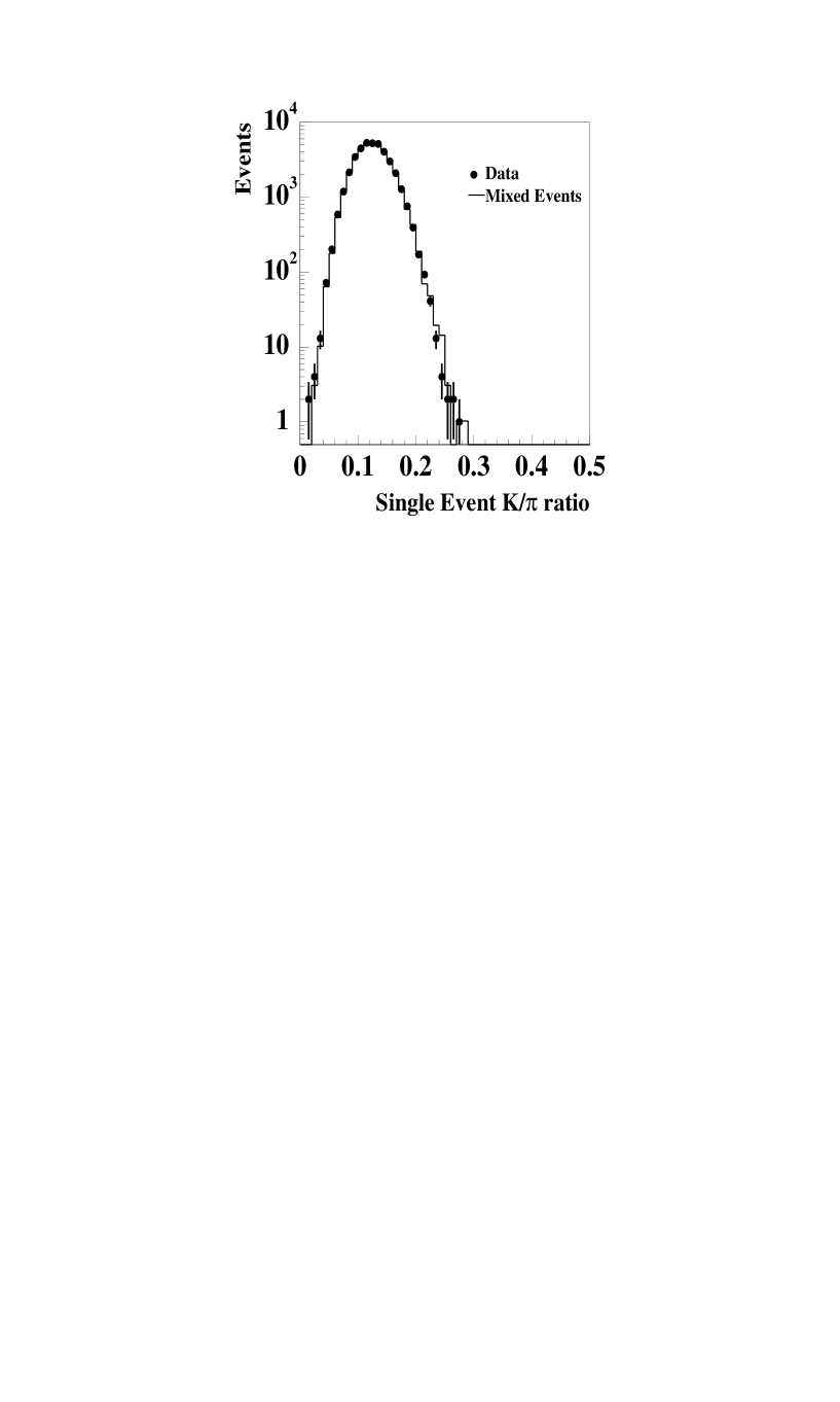
Figure 10: Event-by-event fluctuations in the $K/\pi$ ratio measured by NA49 in central Pb+Pb collisions at the SPS [11].

To second order in the fluctuations of the numbers of K and $\pi$, we have [24, 51]

$$\langle{K/\pi}\rangle=\frac{\langle{K}\rangle}{\langle{\pi}\rangle}\left(1+\frac{\omega_{\pi}}{\langle{\pi}\rangle}-\frac{\langle{K\pi}\rangle-\langle{K}\rangle\langle{\pi}\rangle}{\langle{K}\rangle\langle{\pi}\rangle}\right).$$ (36)

The corresponding fluctuations in $\langle{K/\pi}\rangle$ are given by

$$D^{2}\equiv\frac{\omega_{K/\pi}}{\langle{K/\pi}\rangle}=\frac{\omega_{K}}{\langle{K}\rangle}+\frac{\omega_{\pi}}{\langle{\pi}\rangle}-2\frac{\langle{K\pi}\rangle-\langle{K}\rangle\langle{\pi}\rangle}{\langle{K}\rangle\langle{\pi}\rangle}\,.$$ (37)

The fluctuations in the kaon to pion ratio is dominated by the fluctuations in the number of kaons alone. The third term in Eq. (37) includes correlations between the number of pions and kaons. It contains a negative part from volume fluctuations, which removes the volume fluctuations in $\omega_{K}$ and $\omega_{\pi}$ since such fluctuations cancel in any ratio. In the NA49 data [11] shown in Fig. (10) the average ratio of charged kaons to charged pions is $\langle{K/\pi}\rangle=0.18$ and $\langle{\pi}\rangle\simeq 200$. Excluding volume fluctuations, we take $\omega_{K}\simeq\omega_{\pi}\simeq 1.2-1.3$ as discussed above. The first two terms in Eq. (37) then yield $D\simeq 0.20-0.21$ in good agreement with preliminary measurements $D=0.23$ [11]. Thus at this stage the data gives no evidence for correlated production of K and $\pi$, as described by the final term in Eq. (37), besides volume fluctuations. The similar fluctuations in mixed event analyses $D_{mixed}=0.208$ [11] confirm this conclusion.

Strangeness enhancement has been observed in relativistic nuclear collisions at the SPS. For example, the number of kaons and therefore also $\langle{K/\pi}\rangle$ is increased by a factor of 2-3 in central Pb+Pb collisions. It would be interesting to study the fluctuations in strangeness as well. By varying the acceptance one might be able to gauge the degree of thermalization as discussed above. The fluctuations in the $K/\pi$ ratio as function of centrality would in that case reveal whether strangeness enhancement is associated with thermalization or other mechanisms lie behind. In a plasma of deconfined quarks strangeness is increased rapidly by $gg\to s\bar{s}$ and $q\bar{q}\to s\bar{s}$ processes and lead to enhancement of total strangeness $s+\bar{s}$ whereas the net strangeness $s-\bar{s}$ remains zero. The fluctuations in net and total strangeness will qualitatively behave like net and total charge, however, with unit strangeness quantum numbers as compared to the fractional charges.

5.3 $\pi^{0}/\pi^{\pm}$ ratio and chiral symmetry restoration.

Fluctuations in neutral relative to charged pions would be a characteristic signal of chiral symmetry restoration in heavy ion collisions. If, during expansion and cooling, domains of chiral condensates gets “disoriented” (DCC) [36], anomalous fluctuations in $\pi^{0}/\pi^{\pm}$ ratios could results if DCC domains are large. For single DCC domain the probability distribution of ratios $d=\pi^{0}/(\pi^{0}+\pi^{+}+\pi^{-})$ is $P(d)=1/\sqrt{2d}$ with mean $\langle{d}\rangle=1/3$ and fluctuation $\omega_{d}=4/15$, i.e. much larger than ordinary fluctuations in such ratios (see Eq. (37)) which decrease inversely with the number of pions.

Neutral pions are much harder to measure than charged pions but with respect to fluctuations, it suffices to measure the charged pions only. The anomalous fluctuations in $\pi^{0}$ due to a DCC are anti-correlated to $\pi^{\pm}$, i.e. they are of same magnitude but opposite sign. A DCC can equally well be searched for in total charge fluctuations as in the $\pi^{0}/\pi^{\pm}$ ratio, except for the troublesome impact parameter fluctuations.

5.4 $J/\Psi$ multiplicity correlations and absorption mechanisms

$J/\Psi$ suppression has been found in relativistic nuclear collisions [60] and it is yet unclear how much is due to absorption on participant nucleons and produced particles (comovers). Whether “anomalous suppression” is present in the data is one of the most discussed signals from a hot and dense phase at early times [60]. It was originally suggested that the formation of a quark-gluon plasma would destroy the $c\bar{c}$ bound states [61].

In relativistic heavy ion collisions very few $J/\Psi$’s are produced in each collision. Of these only 6.9% branch into dimuons that can be detected and so the chance to detect two dimuon pairs in the same event is very small. Therefore, it will be correspondingly difficult to measure fluctuations and other higher moments of the number of $J/\Psi$.

Another more promising observable is the correlation between the multiplicities in, e.g., a rapidity interval $\Delta y$ of a charmonium state $\psi=J/\Psi,\psi^{\prime},..$ ($N_{\psi}$) and all particles ($N$) [54]. The correlator $\langle{NN_{\psi}}\rangle-\langle{N}\rangle\langle{N_{\psi}}\rangle$ also enters the in the ratio $\psi/N$ (see Eq. (36)). The correlator has as good statistics as the total number of $\psi$ and it may contain some very interesting anti-correlations, namely that $\psi$ absorption grows with multiplicity $N$. The physics behind can be comover absorption, which grows with comover density, or formation of quark-gluon plasma, which may lead to both anomalous suppression of $\psi$ and large multiplicity in $\Delta y$. Contrarily, direct Glauber absorption should not depend on the multiplicity of produced particles $N$ since it is caused by collisions with participating nucleons.

To quantify this anti-correlation we model the absorption/destruction of $\psi$’s by simple Glauber theory

$$\frac{N_{\psi}}{N_{\psi}^{0}}=e^{-\langle{\sigma_{c\psi}\rho_{c}l}\rangle}\equiv e^{-\gamma N/\langle{N}\rangle}\,,$$ (38)

where $N_{\psi}^{0}$ is the number of $J/\Psi$’s before comover or anomalous absorption sets in but after direct Glauber absorption on participant nucleons. In Glauber theory the exponent is the absorption cross section times the absorber density and path length traversed in matter. The density and therefore also the exponent is proportional to the multiplicity $N$ with coefficient

$$\gamma=-\frac{d\log N_{\psi}}{d\log N}_{|N=\langle{N}\rangle}.$$ (39)

In a simple comover absorption model for a system with longitudinal Bjorken scaling, it can be calculated approximately [62]

$$\gamma\simeq\sum_{c}\frac{dN_{c}}{dy}\frac{\langle{v_{c\psi}\sigma_{c\psi}}\rangle}{4\pi R^{2}}\log R/\tau_{0}\,,$$ (40)

where $dN_{c}/dy$, $\sigma_{c\psi}$, $v_{c\psi}$ and $\tau_{0}$ are the comover rapidity density, absorption cross section, relative velocity and formation time respectively.

On average comover or anomalous absorption is responsible for a suppression factor $e^{-\gamma}$. It is difficult to determine because only the total $\psi$ suppression including direct Glauber absorption on participants is measured.

The anti-correlation is straight forward to calculate when the fluctuations in the exponent are small (i.e. $\gamma\sqrt{\omega_{N}/\langle{N}\rangle}\ll 1$). It is

$$\langle{NN_{\psi}}\rangle-\langle{N}\rangle\langle{N_{\psi}}\rangle=-\gamma\omega_{N}\langle{N_{\psi}}\rangle\,.$$ (41)

It is negative and proportional to the amount of comover and anomalous absorption and obviously vanishes when the absorption is independent of multiplicity ($\gamma=0$). The anti-correlation can be accurately determined as the current accuracy in determining $\langle{N_{\psi}}\rangle$ is a few percent (NA50 minimum bias [60]) in each $E_{T}$ bin.

The anti-correlations in Eq. (41) may seem independent of the rapidity interval. However, if it is less than the typical relative rapidities between comovers and the $\psi$, the correlations disappear. Preferrably, the rapidity interval should be of the order of the typical rapidity fluctuations due to density fluctuations.

The anticorrelations of Eq. (41) quantify the amount of comover or anomalous absorption and can therefore be exploited to distinguish between these and direct Glauber absorption mechanisms. In that respect it is similar to the elliptic flow parameter for $\psi$ [62] for the comover absorption part but differs for the anomalous absorption.

5.5 Photon fluctuations: thermal emission vs. $\pi^{0}\to 2\gamma$

WA98 have measured photon and charged particle multiplicities and their fluctuations versus centrality and $E_{T}$ binning size. As mentioned above impact parameter fluctuations are proportional to the $E_{T}$ binning size; the WA98 analysis nicely confirms this, and can subsequently remove impact parameter fluctuations. The resulting charged particle multiplicity fluctuations with impact parameter fluctuations subtracted, $\omega_{N}-\langle{n}\rangle\omega_{N_{p}}\simeq 1.1-1.2$ were shown in Fig. (7).

The fluctuations in photon multiplicities were found to be almost twice as large as for charged particles $\omega_{\gamma}-\langle{n}\rangle\omega_{N_{p}}\simeq 2.0$. This has the simple explanation that photons mainly are produced in $\pi^{0}\to 2\gamma$ decays. The fluctuations are then the double of the fluctuations in $\pi^{0}$ to first approximation as seen from Eq. (18).

If the photons were directly produced from a “shining” thermal fireball one would expect that they would exhibit Bose-Einstein fluctuations, $\omega_{\gamma}=\omega_{N}^{BE}=1.37$ for massless particles. In addition the $\pi^{0}$’s in the hadronic background will produce photons with $\omega_{\gamma}=\omega_{N}^{BE}=2.0$. The measured fluctuation in the number of photons will therefore lie between these two numbers and can be exploited to quantify the amount of thermal photon emission vs. $\pi^{0}\to 2\gamma$ decay from a hadronic gas

$$\frac{N_{\gamma}^{thermal}}{N_{\gamma}^{thermal}+N_{\gamma}^{\pi^{0}}}=\frac{2.0-\omega_{\gamma}^{exp}}{2.0-1.37}\,.$$ (42)

The impact parameter fluctuations must be subtracted from the measured photon fluctuations $\omega_{\gamma}^{exp}$ by, e.g., taking the ratio of photons to some other particle with known behavior.

6 Transverse momentum fluctuations

Fluctuations in average transverse momentum were among the first event-by-event analyses studied. In a series of papers Mrówczyński et al. have studied transverse momentum fluctuations in heavy-ion collisions with the purpose of studying thermalization and other effects. Fluctuations in temperature and thus average transverse momentum event-by-event were studied by a number of people [15, 16, 17, 18] in connection with critical phenoma relevant if the transition is close to a critical point. Experimental analyses by NA49 [11, 14] reveal that a careful evaluation of systematic effects are required before substantial equilibration can be claimed in central heavy-ion collisions from transverse momentum fluctuations. They also have found strong correlations between multiplicity and transverse momentum.

The total transverse momentum per event

$$P_{t}=\sum_{i=1}^{N}p_{t,i}\,,$$ (43)

is very similar to the transverse energy, for which fluctuations have been studied extensively [10, 8]. The mean transverse momentum and inverse slopes of distributions generally increase with centrality or multiplicity. Assuming that $\alpha\equiv d\log(\langle{p_{t}}\rangle_{N})/d\log N$ is small, as is the case for pions [63], the average transverse momentum per particle for given multiplicity $N$ is to leading order

$$\langle{p_{t}}\rangle_{N}=\langle{p_{t}}\rangle(1+\alpha(N-\langle{N}\rangle)/\langle{N}\rangle)\,.$$ (44)

where $\langle{p_{t}}\rangle$ is the average over all events of the single particle transverse momentum. With this parametrization, the average total transverse momentum per particle in an event obeys $\langle{P_{t}/N}\rangle=\langle{p_{t}}\rangle$. When the transverse momentum is approximately exponentially distributed with inverse slope $T$ in a given event, $\langle{p_{t,i}}\rangle=2T$, and $\sigma(p_{t,i})=2T^{2}=\langle{p_{t}}\rangle^{2}/2$.

The total transverse momentum and also the transverse energy contains both fluctuations in multiplicity and fluctuations in the individual particle transverse momenta and energy (see Appendix C). An interesting quantity is therefore the total transverse momentum per particle, $P_{t}/N$, where the multiplicity fluctuations are removed to first order although important correlations remain.

The total transverse momentum per particle in an event has fluctuations

$$\langle{N}\rangle\sigma(P_{t}/N) = \sigma(p_{t,i})+\alpha^{2}\langle{p_{t}}\rangle^{2}\omega_{N}+\langle{\frac{1}{N}\sum_{i\neq j}(p_{t,i}p_{t,j}-\langle{p_{t}}\rangle^{2})}\rangle\,.$$ (45)

The three terms on the right are respectively:

i) The individual fluctuations $\sigma(p_{t,i})=\langle{p_{t,i}^{2}}\rangle-\langle{p_{t}}\rangle^{2}$, the main term. In the NA49 data, $\langle{p_{t}}\rangle=377$ MeV and $\langle{N}\rangle=270$. From Eq. (45) we thus obtain $(\sigma(P_{t}/N)^{1/2}/\langle{p_{t}}\rangle\simeq 1/\sqrt{2\langle{N}\rangle}=4.3$%, which accounts for most of the experimentally measured fluctuation 4.65% [11]. The data contains no indication of intrinsic temperature fluctuations in the collisions.

ii) Effects of correlations between $p_{t}$ and $N$, which are suppressed with respect to the first term by a factor $\sim\alpha^{2}$. In NA49 the multiplicity of charged particles is mainly that of pions for which $T\simeq\langle{p_{t}}\rangle/2$ increases little compared with pp collisions, and $\alpha\simeq 0.05-0.1$. Thus, these correlations are small for the NA49 data. However, for kaons and protons, $\alpha$ can be an order of magnitude larger as their distributions are strongly affected by the flow observed in central collisions [63].

iii) Correlations between transverse momenta of different particles in the same event. In the WNM the momenta of particles originating from the same participant are correlated. In Lund string fragmentation, for example, a quark-antiquark pair is produced with the same $p_{t}$ but in opposite direction. The average number of pairs of hadrons from the same participant is $\langle{n(n-1)}\rangle$, where $n$ is the number of particles emitted from the same participant nucleon, and therefore the latter term in Eq. (45) becomes $(\langle{n(n-1)}\rangle/\langle{n}\rangle)(\langle{p_{t,i}p_{t,j\neq i}}\rangle-\langle{p_{t}}\rangle^{2})$. To a good approximation, $n$ is Poisson distributed, i.e., $\langle{n(n-1)}\rangle/\langle{n}\rangle=\langle{n}\rangle$, equal to 0.77 for the NA49 acceptance, so that this latter term becomes $\simeq(\langle{p_{t,i}p_{t,j\neq i}}\rangle-\langle{p_{t}}\rangle^{2})$. The momentum correlation between two particles from the same participant is expected to be a small fraction of $\sigma(p_{t,i})$.

To quantify the effect of rescatterings, the difference between $\langle{N}\rangle\sigma(P_{t}/N)$ and $\sigma(p_{t})$ has been studied in detail [12] via the quantity

$$\Phi(p_{t})\simeq\sqrt{\langle{N}\rangle\sigma(P_{t}/N)}-\sqrt{\sigma(p_{t,i})}\,.$$ (46)

As we see from Eq. (45), in the applicable limit that the second and third terms are small,

$$\Phi(p_{t}) \simeq \frac{1}{\sqrt{\sigma(p_{t,i})}}\left(\alpha^{2}\langle{p_{t}}\rangle^{2}\omega_{N}+(\langle{p_{t,i}p_{t,j\neq i}}\rangle-\langle{p_{t}}\rangle^{2})\right)\,.$$

In the Fritiof model, based on the WNM with no rescatterings between secondaries, one finds $\Phi(p_{t})\simeq 4.5$ MeV. In the thermal limit the correlations in Eq. (46) should vanish for classical particles but the interference of identical particles (HBT correlations) contributes to these correlations $\sim 6.5$ MeV [13]; they are again slightly reduced by resonances. The NA49 experimental value, $\Phi(p_{t})=5$ MeV (corrected for two-track resolution) seems to favor the thermal limit [11]. Note however that with $\alpha\simeq 0.05-0.1$, the second term on the right side of Eq. (LABEL:phii) alone leads to $\Phi\simeq 1-4$ MeV, i.e., the same order of magnitude. If $(\langle{p_{t,i}p_{t,j\neq i}}\rangle-\langle{p_{t}}\rangle^{2})$ is not positive, then one cannot a priori rule out that the smallness of $\Phi(p_{t})$ does not arise from a cancellation of this term with $\alpha^{2}\langle{p_{t}}\rangle^{2}\omega_{N}$, rather than from thermalization.

A comparison of the transverse momentum fluctuations of charged particles to those in mixed events, where correlations thus are removed, showed a small enhancement of only $0.002\pm 0.002$ [11]. It was estimated that Bose effects should enhance this ratio by 1-2% but that total energy conservation introduces an anticorrelation that partially cancels the Bose enhancement [17, 18]. Experimental problems with two-track resolution have also been estimated to lead to a ratio that is 1-2% lower. Consequently, the numbers seem to be compatible.

The covariance matrix between multiplicity and transverse momentum has been analyzed by NA49 [11]. Strong but trivial correlations is found due to the fact that higher multiplicity gives larger total transverse momentum event-by-event. This correlation is removed in the quantity $P_{t}/N$ and its covariance matrix with multiplicity appears diagonal.

7 Event-by-Event Fluctuations at RHIC

The theoretical analysis above leads to a qualitative understanding of event-by-event fluctuations and speculations on how phase transitions may show up. It gives a quantitative description of AGS and SPS data without the need to invoke new physics. We shall here look ahead towards RHIC experiments and attempt to describe how fluctuations may be searched for.

General correlators between all particle species should be measured event-by-event, e.g., the ratios [24]

$$\frac{\langle{N_{i}/N_{j}}\rangle}{\langle{N_{i}}\rangle/\langle{N_{j}}\rangle}\simeq 1+\frac{\omega_{N_{j}}}{\langle{N_{j}}\rangle}-\frac{\langle{N_{i}N_{j}}\rangle-\langle{N_{i}}\rangle\langle{N_{j}}\rangle}{\langle{N_{i}}\rangle\langle{N_{j}}\rangle}\,,$$ (48)

where $N_{i,j}$ are the multiplities in acceptances $i$ and $j$ of any particle. Volume fluctuations are automatically removed in such ratios, their fluctuations and correlations. If the energy deposition, transverse energy or momentum are measured, these latter will have additional fluctuation due to the multiplicity fluctuations as explained in Appendix C.

More generally we define the multiplicity correlations between any two bins

$$\omega_{ij}=\frac{\langle{N_{i}N_{j}}\rangle-\langle{N_{i}}\rangle\langle{N_{j}}\rangle}{\sqrt{\langle{N_{i}}\rangle\langle{N_{j}}\rangle}}\,,$$ (49)

also referred to as the covariance. When $i,j$ refer to two rapidity bins the covariance is also proportional to the rapidity (auto-)correlation function $C(y_{i}-y_{j})$.

It is instructive to consider first completely random (uncorrelated or statistical) particle emission. For a fixed total multiplicity $N_{Tot}$, the probability for a particle to end up in bin $i$ is $p_{i}=\langle{N_{i}}\rangle/N_{Tot}\simeq\langle{E_{i}}\rangle/E_{Tot}$. The distribution is a simple multinomial distribution for which

$$\omega_{ij}=\left\{\begin{array}[]{lrl}1-p_{i}&,&i=j\\ -\sqrt{p_{i}p_{j}}&,&i\neq j\end{array}\right\}\,.$$ (52)

The $i=j$ result is the well known one for a binomial distribution. The $i\neq j$ result is negative because particles in different bins are anti-correlated: more (less) particles in one bin leads to less (more) in other bins on average due to a fixed total number of particles.

As shown above there are nonstatistical fluctuations due to various sources: Bose-Einstein fluctuations, resonances, etc., and — in particular — density fluctuations. As in Eq. (21) we assume that the multiplicity consist of particles from a HM and a QM phase. The covariances in Eq. (52) are derived analogously to Eq. (22)

$$\omega_{ij}=\omega_{ij,HM}+(\omega_{ij,QM}-\omega_{ij,HM})\frac{\langle{N_{i,QM}}\rangle}{\langle{N_{i}}\rangle}\,,$$ (53)

when $\langle{N_{i}}\rangle=\langle{N_{j}}\rangle$; when different the general formula is a little more complicated. Now, the hadronic fluctuations $\omega_{ij,HM}$ is of order unity for $i=j$, smaller for adjacent bins and vanishes or even becomes slightly negative according to (52) for bins very different in pseudorapidity or azimuthal angle $\phi$. The QM fluctuations can be much larger: $\omega_{i,QM}\sim\langle{N_{i,QM}}\rangle$ (see the discussion after Eq. (20)). To discriminate the QM fluctuations from the hadronic ones, Eq. (53) requires

$$\langle{N_{i,QM}}\rangle\raisebox{-2.15277pt}{$\stackrel{{\scriptstyle>}}{{\sim}}$}\sqrt{(\omega_{ij}-\omega_{ij,HM})\langle{N_{i}}\rangle}\,.$$ (54)

The charged particle multiplicity in central $Au+Au$ collisions at RHIC is $dN_{ch}/d\eta\simeq 500-600$ per unit pseudo-rapidity [23]. To see a clear increase in fluctuations, say $\Delta\omega\equiv\omega_{ij}-\omega_{ij,HM}\sim 1$, a density fluctuation of only $\langle{N_{i,QM}}\rangle\raisebox{-2.15277pt}{$\stackrel{{\scriptstyle>}}{{\sim}}$}\sqrt{N_{i}}\simeq 25$ particles are required per unit rapidity corresponding to a few percent of the average. By analyzing many events (of the same total multiplicity) the accuracy by which fluctuations are measured experimentally is greatly improved. Generally, $\Delta\omega\sim 1/\sqrt{N_{events}}$, and so fluctuations can in principle be determined with immense accuracy.

It may be advantageous to correlate bins with the same pseudorapidity but different azimuthal angles since the hadronic correlations between these are small whereas QM fluctuations remain.

No experimental determination of the purely statistical uncertainties associated with any one-body distribution — such as multiplicity as a function of rapidity — can be performed without measuring and diagonalizing the correlation matrix $C_{ij}=\langle N_{i}N_{j}\rangle-\langle N_{i}\rangle\langle N_{j}\rangle$. While it is conventional to assign uncertainties according to the diagonal elements $M_{ii}$, the correlations in the covariance matrix are required for a correct error analysis and can also reveal physical important results.

8 Summary

A phase transitions in high energy nuclear collisions, whether it is first order or a soft cross-over, density fluctuations may be expected that show up in rapidity and multiplicity fluctuations event-by-event. The fluctuations can be enhanced significantly in case of droplet formation as compared to that from an ordinary hadronic scenario. A combined analyses of, e.g., positive, negative, total and net charge, allows one to extract the various fluctuations and correlations uniquely. Likewise a number of other observables as charged and neutral pions, kaons, photons, $J/\Psi$, etc., and their ratios can show anomalous correlations and enhancement or suppression of fluctuations. This clearly demonstrates the importance of event-by-event fluctuations accompanying phase transitions, and illustrates how monitoring such fluctuations versus centrality becomes a promising signal, in the upcoming RHIC experiments, for the onset of a transition. The potential for enhanced or suppressed fluctuations (orders of magnitude) from a transition makes it worth looking for at RHIC considering the relative simplicity and accuracy of multiplicity fluctuation measurements.

An analysis of fluctuations in central Pb+Pb collisions as currently measured in NA49 does, however, not show any sign of anomalous fluctuations. Fluctuations in multiplicity, transverse momentum, $K/\pi$ and other ratios can be explained by standard statistical fluctuation and additional impact parameter fluctuations, acceptance cuts, resonances, thermal fluctuations, etc. This understanding by “standard” physics should be taken as a baseline for future studies at RHIC and LHC and searches for anomalous fluctuations and correlations from phase transitions that may show up in a number of observables.

By varying the centrality one should be able to determine quantitatively the amount of thermalization in relativistic heavy ion collisions as defined in Eq. (19) . For peripheral collisions, where only few rescatterings occur, we expect the participant model (WNM) to be approximately valid and the degree of thermalization to be small. For central collisions, where many rescatterings occur among produced particles, we expect to approach the thermal limit and the degree of thermalization should be close to 100%. At RHIC and LHC energies the fluctuations in the number of charged particles consequently decrease drastically with centrality whereas at SPS energies the two limits are accidentally very close.

Event-by-event physics is an important tool to study thermalization and phase transitions through anomalous fluctuations and correlations — as in rain.

Appendix A: Damping of initial density fluctuations

Hydrodynamic flow with Bjorken scaling is stable according to a stability analysis carried out in [35]. Bt linearing the hydrodynamic equations in small perturbations in entropy density $\delta s$ and rapidity $\delta y$ around the Bjorken scaling solution and looking for solutions in the form of harmonic perturbations, $e^{ik\eta}$, the hydrodynamic equations could be written in matrix form (Eq. A.13 in [35])

$$\tau\frac{\delta}{\delta\tau}\left(\begin{array}[]{l}\delta s/s\\ \delta y\end{array}\right)=\left(\begin{array}[]{lll}0&&-ik\\ -ikc_{s}^{2}&&-(1-c_{s}^{2})\end{array}\right)\left(\begin{array}[]{l}\delta s/s\\ \delta y\end{array}\right)\,.$$ (61)

The eigenvalues of the above matrix

$$\lambda_{\pm}=-\frac{1}{2}(1-c_{s}^{2})\pm\sqrt{\frac{1}{4}(1-c_{s}^{2})^{2}-c_{s}^{2}k^{2}}\,,$$ (62)

always have real negative part for $c_{s}k\neq 0$ and fluctuations are therefore damped. For long wave length fluctuations in rapidity and not too soft equations of state, $c_{s}k>1-c_{s}^{2}$, the solution is a damped oscillator. Note that the long wave length solution $k=0$ reproduces the Bjorken scaling.

The exact solution for the entropy density fluctuation

$$\frac{\delta s}{s}=c_{+}e^{\lambda_{+}\ln(\tau/\tau_{0})}+c_{-}e^{\lambda_{-}\ln(\tau/\tau_{0})}\,,$$ (63)

is sensitive to the equation of state through $c_{s}$, the initial conditions for the rapidity density fluctuations (the constants $c_{\pm}$), and their wave length $k^{-1}$.

At large times the eigenvalue with the largest real part dominates and

$$\frac{\delta s}{s}\propto\left(\frac{\tau_{0}}{\tau_{f}}\right)^{|Re[\lambda_{\pm}]|}\,.$$ (64)

Here the oscillating factor has been ignored, leaving the power law fall-off of fluctuations with exponent

$$Min|Re[\lambda_{\pm}]|=\frac{1}{2}(1-c_{s}^{2})-Re[\sqrt{\frac{1}{4}(1-c_{s}^{2})^{2}-c_{s}^{2}k^{2}}]$$ (65)

One notes that density fluctuations are undamped for soft equation of states ($c_{s}=0$). They are also undamped if their wave length is long ($k\simeq 0$).

To estimate the resulting damping we take a typical rapidity fluctuation for a droplet $\delta y\sim\sqrt{T/m_{t}}\sim 1$ discussed above, which corresponds to a wave-number $k\simeq 1$. For an ideal equation of state with sound speed $c_{s}=1/\sqrt{3}$ the last term in Eq. (62) is then either imaginary or small and real, and the real part of the eigenvalue is dominated by the first term of Eq. (62), $Re[\lambda_{\pm}]\simeq-1/3$. If we take a typical formation time $\tau_{0}\simeq 1$ fm/c and a freezeout time $\tau_{f}\simeq 8$ fm/c as extracted from HBT studies [1], the resulting suppression of a density fluctuation during expansion is a factor $\sim 8^{-1/3}=0.5$ according to Eq. (64).

Appendix B: Fluctuations in source models

As fluctuations for a source model appears again and again (see Eqs. 10,11,18,22) we shall derive this simple equation in detail.

We define the fluctuations for any stochastic variable $x$ as

$$\omega_{x}=\frac{\langle{x^{2}}\rangle-\langle{x}\rangle^{2}}{\langle{x}\rangle}\,.$$ (66)

It is usually of order unity and therefore more convenient than variances. For a Poisson distribution, $P_{N}=e^{-\alpha}\alpha^{N}/N!$, the fluctuation is $\omega_{N}=1$. For a binomial distribution with tossing probability $p$ the fluctuation is $\omega_{N}=1-p$, independent of the number of tosses. In heavy ion collisions several processes add to fluctuations so that typically $\omega_{N}^{exp}\sim 1-2$. Correlations can in some cases double the fluctuations as, for example, $\pi^{0}\to 2\gamma$ doubles the fluctuations in photon multiplicity and net charge conservation doubles the fluctuation in total charge. Impact parameter fluctuations further increases the total charge fluctuations to $\omega_{N_{ch}}=3-5$ in peripheral nuclear collisions [64].

Generally, when the multiplicity ($N$) arise from independent sources $(N_{p})$ such as participants, resonances, droplets or whatever,

$$N=\sum_{i=1}^{i=N_{p}}n_{i},$$ (67)

where $n_{i}$ is the number of particles produced in source $i$. In the absence of correlations between $N_{p}$ and $n$, the average multiplicity is $\langle{N}\rangle=\langle{N_{p}}\rangle\langle{n}\rangle$. Here, $\langle{..}\rangle$ refer to averaging over each individual (independent) source as well as the number of sources. The number of sources vary from event to event and average is performed over typically $N_{events}\sim 100.000$ events as in NA49 or $N_{events}\sim 10^{6}$ in WA98.

Squaring Eq. (67) assuming that the source emit particles independently, i.e. $\langle{n_{i}n_{j}}\rangle=\langle{n_{i}}\rangle\langle{n_{j}}\rangle$ for $i\neq j$, the square consists of the diagonal and off-diagonal elements:

$$\langle{N^{2}}\rangle=\langle{N_{p}}\rangle\langle{n_{i}^{2}}\rangle+\langle{N_{p}(N_{p}-1)}\rangle\langle{n_{i}}\rangle^{2}\,.$$ (68)

With (66) we obtain the multiplicity fluctuations

$$\omega_{N}=\frac{\langle{N^{2}}\rangle-\langle{N}\rangle^{2}}{\langle{N}\rangle}=\omega_{n}+\langle{n}\rangle\omega_{N_{p}},$$

as in Eq. (10).

Appendix C: Fluctuations in the energy deposited

Many experiments do not measure individual particle tracks or multiplicities but instead the energy deposited in arrays of detector segments, $E_{i}$, in a given event. One could also project the energy transversely by weighting with the sine of the scattering angle to study fluctuations in transverse energy [7, 8, 9, 10]. Since particles mostly have relativistic speeds in relativistic heavy-ion collisions, the transverse energy is almost the same as the total transverse momentum in an event.

The total energy deposited in the event is

$$E_{Tot}=\sum_{i}^{D}E_{i}\,,$$ (69)

and can be used as a measure of the centrality of the collision. The energy deposited in each element (or group of elements) is the sum over the number of particle tracks ($N_{i}$) hitting detector $i$ of the individual ionization energy of each particle ($\epsilon_{i}$)

$$E_{i}=\sum_{n}^{N_{i}}\epsilon_{n}\,.$$ (70)

The average is: $\langle{E_{i}}\rangle=\langle{N_{i}}\rangle\langle{\epsilon}\rangle$. The energy will approximately be gaussian distributed, $d\sigma/dE_{i}\propto\exp(-(E_{i}-\langle{E_{i}}\rangle)^{2}/2\omega_{E_{i}}\langle{E_{i}}\rangle)$, with fluctuations (see Appendix B)

$$\omega_{E_{i}}\equiv\frac{{\langle{E_{i}^{2}}\rangle-\langle{E_{i}}\rangle^{2}}}{\langle{E_{i}}\rangle}=\omega_{\epsilon}+\langle{\epsilon}\rangle\omega_{N_{i}}\,.$$ (71)

Here, the fluctuation in ionization energy per particle

$$\frac{\omega_{\epsilon}}{\langle{\epsilon}\rangle}=\frac{\langle{\epsilon^{2}}\rangle}{\langle{\epsilon}\rangle^{2}}-1\,,$$ (72)

depends on the typical particle energies in the detector and the corresponding ionization energies for the detector type and thickness. For the BRAHMS detectors we estimate $\omega_{\epsilon}/\langle{\epsilon}\rangle\simeq 0.3$ [65]. This number will, however, depend on rapidity since the longitudinal velocity enters the ionization power. As these are “trivial” detector parameter, we shall exclude the fluctuations $\omega_{\epsilon}$ in most analyses and concentrate on the second term in Eq. (71) which is the fluctuations in the number of particles as examined in detail above.

References

- [1] R. Hanbury–Brown and R.Q. Twiss, Phil. Mag. 45 (1954) 633. S. Pratt, Phys. Rev. Lett. 53 (1984) 1219. T. Csörgő and B. Lörstad, Phys. Rev. C54 (1996) 1390. U. Heinz and B.V. Jacak, Ann. Rev. Nucl. Part. Sci. 49 (1999), and references therein.
- [2] S. Trentalange and S.U. Pandey, J. Acoust. Sci. Am. 99 (1996) 2439; C. Slotta and U. Heinz, Phys. Rev. E 58 (1998) 526.
- [3] M.R. Andrews, C.G. Townsend, H.-J. Miesner, D.S. Durfee, D. M. Kurn, and W. Ketterle, Science 275 (1997) 637; Y. Castin and J. Dalibard, Phys. Rev. A 55 (1997) 4330.
- [4] See, e.g., J. Phillips et al., astro-ph/0001089.
- [5] M. Toscano et al., Mon. Not. R. Astron. Soc., astro-ph/9811398.
- [6] P. Braun-Munziger and J. Stachel, Nucl. Phys. A638 (1998) 3c, and refs. herein.
- [7] G. Baym, G. Friedman, and I. Sarcevic, Phys. Lett. 219B (1989) 205.
- [8] H. Heiselberg, G.A. Baym, B. Blättel, L.L. Frankfurt, and M. Strikman, Phys. Rev. Lett. 67 (1991) 2946; B. Blättel, G.A. Baym, L.L. Frankfurt, H. Heiselberg and M. Strikman, Nucl. Phys. A544 (1992) 479c.
- [9] G. Baym, B. Blättel, L. L. Frankfurt, H. Heiselberg, and M. Strikman, Phys. Rev. C 52 (1995) 1604.
- [10] T. Åkesson et al. (Helios collaboration), Z. Phys. C38 (1988) 383.
- [11] G. Roland et al., (NA49 collaboration), Nucl. Phys. A638, 91c (1998); H. Appelhäuser et al., (NA49 collaboration), Phys. Lett. B459 (1999) 679; J.G. Reid, (NA49 collaboration), Nucl. Phys. A 661 (1999) 407c; K. Perl, NA49 note 244.
- [12] M. Gaździcki and S. Mrówczyński, Z. Phys. C54 (1992) 127.
- [13] S. Mrówczyński, Phys. Rev. C 57 (1998) 1518; Phys. Lett. B430, 9; ibid. B439 (1998) 6; ibid. B465 (1999) 8; Acta Phys.Polon. B31 (2000) 2065
- [14] T.A. Trainor, hep-ph/0001148; T.A. Trainor and J.G. Reid, hep-ph/0004258.
- [15] L. Stodolsky, Phys. Rev. Lett. 75 (1995) 1044.
- [16] E. V. Shuryak, Phys. Lett. B430 (1998) 9.
- [17] M. Stephanov, K. Rajagopal, and E. Shuryak, Phys. Rev. Lett. 81, 4816 (1998); Phys. Rev. D60 (1999) 114028; K. Rajagopal, proc. of the Minnesota conference on Continuous Advances in QCD 1998 (hep-th/9808348).
- [18] B. Berdnikov and K. Rajagopal, Phys. Rev. D. 61, 105017 (2000); K. Rajagopal, proc. of International Conference on Quark Nuclear Physics, Adelaide, Australia, Feb. 2000 (hep-ph/0005101).
- [19] S. Gavin and C. Pruneau, nucl-th/9907040; S. Gavin, nucl-th/9908070.
- [20] S.A. Voloshin, V. Koch, H.G. Ritter, nucl-th/9903060.
- [21] A. Bialas and R. Peschanski, Nucl. Phys. B273 (1986) 703.
- [22] M.A. Bloomer et al. (WA80), Nucl. Phys. A544 (1992) 543c.
- [23] B.B. Back et al. PHOBOS Collaboration, Phys. Rev. Lett. 85 (2000) 3100.
- [24] G. Baym and H. Heiselberg, Phys. Lett. B469 (1999) 7.
- [25] L. Van Hove, Phys. Lett. 118B (1982) 138.
- [26] C. Bernard et al., Phys.Rev. D55 (1997) 6861; Y. Iwasaki, K. Kanaya, S. Kaya, S. Sakai, T. Yoshi , Phys. Rev. D 54 (1996) 7010.
- [27] G. Boyd et al, Phys. Rev. Lett. 75 (1995) 4169. E. Laermann, Proc. Quark Matter ’96, Nucl. Phys. A610 (1996) 1c.
- [28] JLQCD Collaboration, Nucl. Phys. Proc. Suppl. 73 (1999) 459.
- [29] K. Eskola, hep-ph/9911350.
- [30] L.D. Landau & E.M. Lifshitz, Statistical Physics, Part 1 (Pergamon, 1980).
- [31] L. Van Hove, Z. Phys. C21 (1984) 93; J.I. Kapusta, A.P. Vischer, Phys. Rev. C52 (1995) 2725; E.E. Zabrodin, L.P. Csernai, J.I. Kapusta, G. Kluge, Nucl. Phys. A566 (1994) 407c.
- [32] H. Heiselberg, C. J. Pethick and E. F. Staubo, Phys. Rev. Lett. 70 (1993) 1355.
- [33] M.A. Halasz, A.D. Jackson, R.E. Shrock, M.A. Stephanov, J.J.M. Verbaarschot, Phys. Rev. D 58 (1998) 96007.
- [34] H. Heiselberg and A.D. Jackson, Proc. Adv. in QCD, Minnesota, May 1998, nucl-th/9809013.
- [35] G. Baym, B.L. Friman, J.-P. Blaizot, M. Soyeur, W. Czyz, Nucl. Phys. A407 (1983) 541.
- [36] J. Bjorken, Phys. Rev. D27 (1983) 140; M. Alford, K. Rajagopal and F. Wilczek, Phys. Lett. B422 (1998) 247; Nucl. Phys. B558 (1999) 219
- [37] A. Bialas, M. Bleszynski and W. Czyz, Nucl. Phys. B111 (1976) 461.
- [38] K. Werner, private communication.
- [39] W. Thome et al., Nucl. Phys. B129 (1977) 365.
- [40] J. Whitmore, Phys. Rep. 27 (1976) 187.
- [41] UA5 Collaboration, G. J. Alner et al., Z. Phys. C33 (1986) 1; Phys. Rep. 154 (1987) 247.
- [42] H. Bøggild and T. Ferbel, Ann. Rev. Nucl. Sci. 24 (1974) 451.
- [43] E735 Collaboration, C. S. Lindsey et al., Nucl. Phys. A 544 (1992) 343c.
- [44] Z. Koba, H. B. Nielsen and P. Olesen, Nucl. Phys. B40 (1972) 317.
- [45] E877 coll., J. Barrette et al., Phys. Rev. C56 (1997) 3254; E895 coll., H. Liu et al., A638 (1998) 451c.
- [46] M. Gazdzicki & O. Hansen, Nucl. Phys. A528 (1991) 754; W. Wroblewski, Acta Phys. Pol. B4 (1973) 857.
- [47] J. Schukraft et al. (NA34 collaboration), Nucl. Phys. A498 (1989) 79c.
- [48] H. Heiselberg and A. Levy, Phys. Rev. C59 (1999) 2716.
- [49] T.K. Nayak (WA98 collaboration), private communication.
- [50] G. Bertsch, Phys. Rev. Lett. 72 (1994) 2349.
- [51] S. Jeon and V. Koch, Phys.Rev.Lett. 83 (1999) 5435
- [52] M. Asakawa, U. Heinz, and B. Müller, Phys.Rev.Lett. 85 (2000) 2072.
- [53] S. Jeon and V. Koch, Phys. Rev. Lett. 85 (2000) 2076.
- [54] H. Heiselberg and A.D. Jackson, nucl-th/0006021.
- [55] J. Sollfrank, P. Koch, and U. Heinz, Z. Phys. C 52 (1991) 593; J. Sollfrank, U. Heinz, Phys. Lett. B 289 (1992) 132; G.E. Brown, J. Stachel, and G.M. Welke, Phys. Lett. B253 (1991) 19.
- [56] J. P. Sullivan et al., Phys. Rev. Lett. 70 (1993) 3000.
- [57] H. Heiselberg, Phys. Lett. B379 (1996) 27. U.A. Wiedemann and U. Heinz, Phys. Rev. C56 (1997) 3265.
- [58] M. Bleicher, S. Jeon, V. Koch, Phys.Rev. C62 (2000) 061902.
- [59] M. Stephanov and E. Shuryak, hep-ph/0010100.
- [60] NA50 Collaboration, M.C. Abreu et al., Phys. Lett. B410, 327 (1997); ibid 337; CERN-EP/99-13, to appear in Phys. Lett. B.
- [61] T. Matsui and H. Satz, Phys. Lett. 178B (1991) 416
- [62] H. Heiselberg and R. Mattiello, Phys. Rev. C 60 (1999) 44902
- [63] I.G. Bearden et al. (NA44 collaboration), Phys. Rev. Lett. 78 (1997) 2080.
- [64] S. Voloshin (NA49), private comm.
- [65] J.J. Gaardhøje, BRAHMS collaboration, priv. comm.