[

Momentum conservation and local field corrections for the response of interacting Fermi gases

Abstract

We reanalyze the recently derived response function for interacting systems in relaxation time approximation respecting density, momentum and energy conservation. We find that momentum conservation leads exactly to the local field corrections for both cases respecting only density conservation and respecting density and energy conservation. This rewriting simplifies the former formulae dramatically. We discuss the small wave vector expansion and find that the response function shows a high frequency dependence of $\omega^{-5}$ which allows to fulfill higher order sum rules. The momentum conservation also resolves a puzzle about the conductivity which should only be finite in multicomponent systems.

]

Recently the improvement of the response function in interacting quantum systems has regained much interest [1, 2]. This quantity is important in a variety of fields and describes the induced density variation if the system is externally perturbed: $\delta n=\chi V^{\rm ext}$. As an example for an interacting system with potential $V$ the conductivity can be calculated from the response function via

$${\rm Re}\sigma=-{V\over 4\pi}\omega{\rm Im}\chi.$$ (1)

One of the most fruitful concepts to improve the response functions including correlations are the local field corrections $G$

$$\chi={\chi_{0}\over 1+G\chi_{0}},$$ (2)

see [1, 3, 4] and references therein.

On the other hand there exists an extremely useful form of the response function when the interactions are abbreviated in the relaxation time approximation $\tau$ respecting density conservation[5]. One of the advantages of the resulting Mermin formula (11) is that it leads to the Drude -like form of the dielectric function in the long wavelength limit

$$\epsilon=1-V\chi=1-{\omega_{p}^{2}\over\omega(\omega+{i\over\tau})}$$ (3)

with the plasma frequency $\omega_{p}$ for the Coulomb potential $V$ from which follows the conductivity

$${\rm Re}\sigma={ne^{2}\tau\over m(1+\omega^{2}\tau^{2})}=\left\{\matrix{{ne^{2}\tau\over m}+o(\omega)\cr{ne^{2}\over m\omega^{2}\tau}+o({1\over\omega})}\right..$$ (4)

However one should note that this formula is valid only for the extension to a multicomponent system [6] (at least a two-component system) since it makes no sense to speak of conductivity in a single component system where the conductivity should be infinite. Clearly the Mermin formula does not distinguish these cases and cannot be sufficient to describe the response. Therefore we will show that the inclusion of additional momentum conservation will repair this defect (39) and will lead to a conductivity

$${\rm Re}\sigma={ne^{2}\tau\over m(1+\omega^{2}\tau^{2})}{nq^{2}\over m\omega^{2}}\left({1\over\partial_{\mu}n}-{2E\over n^{2}}\right)$$ (5)

which shows indeed for the static limit a diverging behavior in contrast to (4).

There are two distinguishable cases, the single component case where we have to include momentum conservation and obtain divergent conductivity and the multicomponent case where we should expect Mermin-like formulae in order to render the conductivity finite. In order to bring these two extreme cases together the response function for multicomponent systems should be considered [6].

In this letter we want to restrict to the one - component situation. In [2] we have derived the density, current and energy response $\chi,\chi_{J},\chi_{E}$ of an interacting quantum system

$$\left(\matrix{\delta n\cr\delta{\bf\nabla J}\cr\delta E}\right)=\left(\matrix{\chi\cr\chi_{J}\cr\chi_{E}}\right)\,\,V^{\rm ext}\equiv{\cal X}\left(\matrix{1\cr 0\cr 0}\right)V^{\rm ext}\equiv{\cal X}\nu^{\rm ext}$$ (6)

(7)

to the external perturbation $V^{\rm ext}$ provided the density, momentum and energy are conserved. The interacting system has been described by the quantum kinetic equation for the density operator in relaxation time approximation where the relaxation is considered with respect to the local density operator or the corresponding local equilibrium distribution function. This local equilibrium is given by a local chemical potential $\mu$, a local temperature $T$ and a local momentum $Q$ of mass motion. These local quantities are specified by the requirement that the expectation values for density, momentum and energy are the same when calculated from local distribution function or performed with the density operator.

The density response functions have been expressed in [2] for the inclusion of successively more conservation laws in terms of polarization functions ${\cal P}=\{\Pi,\Pi_{n},\Pi_{E}\}$ and have the general form

$${\cal X}={\cal P}(1-{\cal V}{\cal P})^{-1}$$ (8)

due to the induced mean fields which can have density - and momentum - dependent Skyrme form.

When we note the free response function or Lindhard polarization function without collisions as

$$\Pi_{0}=s\int{d{\bf p}\over(2\pi)^{3}}{f_{0}({\bf p}+{{\bf q}\over 2})-f_{0}({\bf p}-{{\bf q}\over 2})\over{{\bf pq}\over m}-\omega-i0}$$ (9)

with finite temperature Fermi functions $f_{0}$, the inclusion of only density conservation leads to the Mermin polarization [5]

$$\Pi^{\rm n}({\bf q},\omega) = \frac{\displaystyle\Pi_{0}({\bf q},\omega+{i/\tau})}{\displaystyle 1-\frac{1}{1-i\omega\tau}\left[1-\frac{\Pi_{0}({\bf q},\omega+{i/\tau})}{\Pi_{0}({\bf q},0)}\right]}$$ (10)

$$= (1-i\omega\tau){g_{1}(\omega+{i\over\tau})g_{1}(0)\over h_{1}}.$$ (11)

If we include also the energy conservation we obtain [2] an additional term to (11)

$$\Pi^{\rm n,E}(\omega) = (1-i\omega\tau)\left({g_{1}(\omega+{i\over\tau})g_{1}(0)\over h_{1}}\right.$$ (13)

$$\left.-\omega\tau i{(h_{\epsilon}g_{1}(0)-h_{1}g_{\epsilon}(0))^{2}\over h_{1}(h_{\epsilon}^{2}-h_{\epsilon\epsilon}h_{1})}\right)$$

where we use the abbreviation

$$h_{\phi}=g_{\phi}(\omega+{i\over\tau})-\omega\,\tau\,i\,g_{\phi}(0).$$ (14)

The different occurring correlation functions can be written in terms of moments of the usual Lindhard polarization function (9) as follows [2]:

$$g_{1} = \Pi_{0},$$ (15)

$$g_{\epsilon} = -{n\over 2}+{m\omega^{2}\over 2q^{2}}\Pi_{0}+{1\over 2m}\tilde{\Pi}_{2},$$ (16)

$$g_{\epsilon\epsilon} = -{7\over 6}{E}-{nq^{2}\over 16m}(1+{4m^{2}\omega^{2}\over q^{4}})-{m^{2}\omega^{4}\over 4q^{4}}\tilde{\Pi}_{0}$$ (18)

$$-{\omega^{2}\over 2q^{2}}\tilde{\Pi}_{2}-{1\over 4m^{2}}\tilde{\Pi}_{4}.$$

Integration via the chemical potential yields the higher moments of the polarization function

$$\tilde{\Pi}_{2} = 2m\int\limits_{-\infty}^{\mu}d\mu^{\prime}\Pi_{0},$$ (19)

$$\tilde{\Pi}_{4} = 2(2m)^{2}\int\limits_{-\infty}^{\mu}d\mu^{\prime}\int\limits_{-\infty}^{\mu^{\prime}}d\mu^{\prime\prime}\Pi_{0}$$ (20)

and the density and energy are given by

$$n = \int{dp\over(2\pi\hbar)^{3}}f_{0}(p),$$ (21)

$$E = \int{dp\over(2\pi\hbar)^{3}}{p^{2}\over 2m}f_{0}(p).$$ (22)

For the inclusion of additional momentum conservation to formulae (11) or (13) we obtain now a tremendous simplification by observing that the formulae given in [2] can be rewritten as

$${1\over\Pi^{\rm n,j}(\omega)}-{1\over\Pi^{\rm n}(\omega)} = {1\over\Pi^{\rm n,j,E}(\omega)}-{1\over\Pi^{\rm n,E}(\omega)}$$ (23)

$$= -{i\omega\over\tau}{m\over nq^{2}}\equiv G.$$ (24)

This shows that the inclusion of momentum conservation leads to nothing but the local field correction with the same form $G$ for both cases, the inclusion of only density conservation and additional energy conservation. Formula (24) is the main result of this paper since it leads to a tremendous simplification. To see the advantages more clearly we discuss now limiting cases.

The long wave length expansion is particularly important for the classical limit and for the discussion of sum rules [7]. Since the discussion above has shown the advantage of discussing the inverse polarization function instead of the polarization function itself we proceed and give the expansion for the inverse polarization functions (9), (11) and (13)

$${1\over\Pi_{0}} = {m\omega^{2}\over nq^{2}}-{2E\over n^{2}}+o(q^{2}),$$ (25)

$${1\over\Pi^{\rm n}} = {m\omega(\omega+{i\over\tau})\over nq^{2}}-\left({i\over\omega\tau}{1\over\partial_{\mu}n}+{2E\over n^{2}}\right){\omega\over\omega+{i\over\tau}}+o(q^{2}),$$ (26)

$${1\over\Pi^{\rm n,E}} = {1\over\Pi_{\rm n}}-{nq^{2}\over 18m}\left({9\over\partial_{\mu}n}-{10E\over n^{2}}\right)^{2}{\omega\over(\omega+{i\over\tau})^{3}}+o(q^{4}).$$ (27)

From equations (24) it is straight forward to derive the expansions for $\Pi^{\rm nj}$ and $\Pi^{\rm njE}$.

The first observation is that up to zeroth order in $q$ the local field corrections (24) induced by momentum conservation lead to an exact cancellation of the effect of collisions in (11) since we have

$${1\over\Pi^{\rm n}}-{1\over\Pi_{0}}=-G+o(q^{0})$$ (29)

which shows that we have to go to the next order in $q$ as done in (LABEL:nn).

Also one recognizes that the inclusion of energy conservation leads only to corrections in next order of $q^{2}$ with respect to $\Pi^{\rm n}$. Moreover, we observe that this correction even vanishes if we employ the zero temperature limit. For zero temperature we have $E=3\epsilon_{f}n/5$ and $\partial_{\mu}n=3n/2\epsilon_{f}$ with the Fermi energy $\epsilon_{f}$ such that

$${1\over\Pi^{\rm njE}} = {1\over\Pi^{\rm nj}}+o(q^{4})$$ (30)

$$= {m\omega^{2}\over nq^{2}}-{2\epsilon_{f}\over 15n}{9\omega+{5i\over\tau}\over\omega+{i\over\tau}}+o(q^{4}).$$ (31)

Using (LABEL:nn) one can write all the effects of correlation including conservation laws in one common local field factor

$$\tilde{G} = {1\over\Pi^{\rm n,j,E}}-{1\over\Pi_{0}}$$ (32)

$$= -{1\over 1-i\omega\tau}\left({1\over\partial_{\mu}n}-{2E\over n^{2}}\right)+o(q^{2})$$ (33)

$$= {1\over 1-i\omega\tau}{8\epsilon_{f}\over 15n}+o(q^{4})$$ (34)

where the last line is valid for zero temperature.

This allows in turn to give the small wave vector expression of the polarization function itself in a Drude-like expression

$$\lim_{{\bf q}\to 0}\Pi^{\rm n,j,E}({\bf q},\omega)=\frac{nq^{2}}{m\omega\left[\omega+{nq^{2}\over m\omega}{\rm Re}\tilde{G}(\omega)+{i\over\tilde{\tau}(\omega)}\right]}$$ (35)

with the modified frequency–dependent relaxation rate

$$\tilde{\tau}^{-1}={nq^{2}\over m\omega}{\rm Im}\tilde{G}(\omega)$$ (37)

similar to [1]. The advantage here is that we have simple explicit formulae for the dynamical local field factor $\tilde{G}$ and the modified relaxation rate while in [1, 8] this could only be given in static approximation and involving complicated integrals. If we had used simply the Mermin formula (11) we would have obtained $\tilde{\tau}=\tau$ and ${\rm Re}\tilde{G}=0$.

In particular we find for the imaginary part

$$\lim_{\omega\to\infty}{\rm Im}\Pi^{\rm n,j,E}({\bf q},\omega) = -\frac{n^{2}q^{4}}{\omega^{5}\tau m^{2}}\left({1\over\partial_{\mu}n}-{2E\over n^{2}}\right)$$ (38)

$$= -\frac{8\epsilon_{f}nq^{4}}{15\omega^{5}\tau m^{2}},$$ (39)

$$\lim_{\omega\to\infty}{\rm Im}\Pi^{\rm n}({\bf q},\omega) = -\frac{n^{2}q^{4}}{\omega^{3}\tau m^{2}}$$ (40)

showing a characteristic different high frequency behavior. While in [2] we have checked the improved convergence of first energy weighted sum rule for the full expression (24) we want to point out that the $\omega^{-5}$ decrease for high frequencies allows to fulfill higher order sum rules. The analytical discussion and proof similar to [7] will be devoted to a forthcoming work.

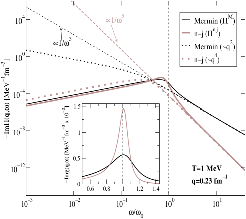
In Fig. 1 we compare the imaginary part of the polarization function for the density and momentum approximation (gray lines) with the Mermin (density) approximation (dark lines) as function of energy with the corresponding limiting cases.

First we want to discuss the corresponding complete expressions (solid lines) of the Mermin formula (11) and the formula (24) including momentum, density and energy conservation. One recognizes that the low frequency limit agrees between Mermin (density) formula and the complete formula while the high frequency limit shows the characteristic different behavior of $\omega^{-3}$ for Mermin (40) and a stronger decrease of $\omega^{-5}$ for the complete expression as have been seen in (39). The high frequency expressions according to (39) and (40) are given by corresponding dashed lines in the figure.

Let us now examine the long–wave length limits (35) of the Mermin formula (11) and the one including momentum, density and energy conservation (24) plotted in the figure as dotted lines. We see that the long wave limit of the Mermin formula approximates the high frequency behavior of the Mermin formula (11) nicely but fails for low frequencies. In contrast, the long wave length expansion of the expression including momentum conservations (35) shows an excellent agreement with the complete expression (24) for both the high and low frequency limit. Please remember that in the latter expression (35) the corrections of order $q^{2}$ drop out and it is effectively of the order $q^{4}$. The nice numerical agreement of the expression (35) with the full result (24) underlines also the force of local field corrections in constructing approximate formulae for the response functions.

FIG. 1.: The imaginary part of the polarization function versus scaled energy for the Mermin formula (11) respecting only density conservation (black solid line) compared with the full expression (24) respecting energy, momentum and density conservation (gray solid line). As an exploratory example hot symmetric nuclear matter ($T=1$ MeV, $n_{0}=0.16{\rm fm}^{-3}$) with the wave vector $q=0.23{\rm fm}^{-1}$ corresponding to $Pb$ has been chosen. Similar figures are obtained for plasma systems. The imaginary part of the response function is depicted in the inlay without logarithmic plot. The long wave length expansions for the Mermin (11) and the complete formula (24) are given by corresponding dotted lines. To guide the eye the high frequency limits (40) and (39) are given by long dashed lines.

The valuable comments by J. D. Frankland (GANIL) are gratefully acknowledged.