Double giant dipole resonances in time-dependent density-matrix theory

Abstract

The strength functions of the double giant dipole resonances (DGDR) in ¹⁶O and ⁴⁰Ca are calculated with the use of an extended version of the time-dependent Hartree-Fock theory known as the time-dependent density-matrix theory. The calculations are done in a self-consistent manner, in which the same Skyrme force as that used for a mean-field potential is used as an effective interaction for a two-body correlation function. It is found that the DGDR in ¹⁶O has a large width due to the Landau damping, although the centroid energy of the strength distribution is close to twice the energy of the giant dipole resonance (GDR) calculated in RPA. The DGDR in ⁴⁰Ca is found more harmonic than that in ¹⁶O: the strength function of the DGDR in ⁴⁰Ca is similar to what is predicted from the strength function of the GDR in RPA.

PACS numbers: 21.60.Jz, 24.10.Cn, 24.30.Cz

Keywords: giant dipole resonance, double phonon state, extended time-dependent Hartree-Fock theory

The double phonon states of giant resonances have become the subject of a number of recent experimental and theoretical investigations [1, 2]. Microscopic calculations of the strength functions of double giant dipole resonances (DGDR) have also been done based on the shell model [3, 4] and quasiparticle-phonon models [2, 5]. However, few microscopic studies have been reported, in which a single-particle basis and a residual interaction are treated in such a self-consistent manner as used in random-phase-approximation (RPA) calculations for giant resonances [6]. We have recently proposed a self-consistent approach [7] based on an extended version of the time-dependent Hartree-Fock theory (TDHF) known as the time-dependent density-matrix theory (TDDM) [8], in which the same Skyrme force as that used for the calculation of a mean-field potential is used as a residual interaction for a two-body correlation function. We applied the model to the double giant quadrupole resonances (DGQR) in ¹⁶O and ⁴⁰Ca [9] and showed that the DGQR’s in these nuclei have strong harmonic properties. The aim of this paper is to report the results of the application of the TDDM approach to the DGDR’s in ¹⁶O and ⁴⁰Ca.

The formulation of TDDM is based on the truncation of the hierarchy of reduced density matrices, in which genuine correlated parts in a three-body density matrix and higher reduced density matrices are neglected [10]. The TDDM equations thus determine the time evolution of a one-body density matrix $\rho$ and a two-body correlation function $C_{2}$ defined by $C_{2}=\rho_{2}-A[\rho\rho]$, where $A[\rho\rho]$ is the antisymmetrized product of the one-body density matrices and $\rho_{2}$ is a two-body density matrix. In TDDM, further truncation is made by expanding $\rho$ and $C_{2}$ with a finite number of single-particle states $\{\psi_{\alpha}\}$ as

$$\rho(11^{\prime},t) = \sum_{\alpha\alpha^{\prime}}n_{\alpha\alpha^{\prime}}(t)\psi_{\alpha}(1,t)\psi_{\alpha^{\prime}}^{*}(1^{\prime},t),$$ (1)

$$C_{2}(121^{\prime}2^{\prime},t)=\sum_{\alpha\beta\alpha^{\prime}\beta^{\prime}}C_{\alpha\beta\alpha^{\prime}\beta^{\prime}}(t)\psi_{\alpha}(1,t)\psi_{\beta}(2,t)\psi_{\alpha^{\prime}}^{*}(1^{\prime},t)\psi_{\beta^{\prime}}^{*}(2^{\prime},t),$$ (2)

where the numbers denote space, spin and isospin coordinates. The time evolution of $\rho$ and $C_{2}$ is determined by the following three coupled equations [8]:

$$i\hbar\frac{\partial}{\partial t}\psi_{\alpha}(1,t)=h(1,t)\psi_{\alpha}(1,t),$$ (3)

$$i\hbar\dot{n}_{\alpha\alpha^{\prime}}=\sum_{\beta\gamma\delta}[\langle\alpha\beta|v|\gamma\delta\rangle C_{\gamma\delta\alpha^{\prime}\beta}-C_{\alpha\beta\gamma\delta}\langle\gamma\delta|v|\alpha^{\prime}\beta\rangle],$$ (4)

$$i\hbar\dot{C}_{\alpha\beta\alpha^{\prime}\beta^{\prime}}=B_{\alpha\beta\alpha^{\prime}\beta^{\prime}}+P_{\alpha\beta\alpha^{\prime}\beta^{\prime}}+H_{\alpha\beta\alpha^{\prime}\beta^{\prime}},$$ (5)

where $h(1,t)$ is the mean-field hamiltonian and $v$ the residual interaction. The term $B_{\alpha\beta\alpha^{\prime}\beta^{\prime}}$ on the right-hand side of Eq.(5) represents the Born terms (the first-order terms of $v$). The terms $P_{\alpha\beta\alpha^{\prime}\beta^{\prime}}$ and $H_{\alpha\beta\alpha^{\prime}\beta^{\prime}}$ in Eq.(5) contain $C_{\alpha\beta\alpha^{\prime}\beta^{\prime}}$ and represent higher-order particle-particle (and hole-hole) and particle-hole type correlations, respectively. Thus full two-body correlations including those induced by the Pauli exclusion principle are taken into account in the equation of motion for $C_{\alpha\beta\alpha^{\prime}\beta^{\prime}}$. The explicit expressions for $B_{\alpha\beta\alpha^{\prime}\beta^{\prime}}$, $P_{\alpha\beta\alpha^{\prime}\beta^{\prime}}$ and $H_{\alpha\beta\alpha^{\prime}\beta^{\prime}}$ are given in Ref.[8]. The small amplitude limit of TDDM was investigated [11] and it was shown that TDDM can be reduced to the second RPA [12]-[14] in such a limit. The number of two-body matrices treated in TDDM grows very rapidly with increasing mass number, restricting the application of TDDM to light nuclei for the present. To solve the coupled equations, we use the Skyrme interaction of the form [15]

$$v({\bf r}-{\bf r^{\prime}}) = t_{0}(1+x_{0}P_{\sigma})\delta^{3}({\bf r}-{\bf r^{\prime}})+\frac{1}{2}t_{1}\{k^{\prime 2}\delta^{3}({\bf r}-{\bf r^{\prime}})+\delta^{3}({\bf r}-{\bf r^{\prime}})k^{2}\}$$ (6)

$$+ t_{2}{\bf k^{\prime}}\cdot\delta^{3}({\bf r}-{\bf r^{\prime}}){\bf k}+\frac{1}{2}t_{3}\rho\left(\frac{{\bf r}+{\bf r^{\prime}}}{2}\right)\delta^{3}({\bf r}-{\bf r^{\prime}}),$$ (7)

where ${\bf k}=(\nabla_{\bf r}-\nabla_{\bf r^{\prime}})/2i$ acts to the right and ${\bf k^{\prime}}=(\nabla_{\bf r^{\prime}}-\nabla_{\bf r})/2i$ acts to the left. The factor 1/2 on the density dependent term contains the contribution of a rearrangement effect [15]. We use the parameter set of the Skyrme III force (SKIII) [16]. The spin-orbit force is neglected. We assume that the motion of the DGDR is generated by a two-body operator $\hat{D}^{2}$:

$$|\Psi(t=0)\rangle=e^{ik\hat{D}^{2}}|\Phi_{0}\rangle,$$ (8)

where $\hat{D}$ is a one-body dipole operator and $|\Phi_{0}\rangle$ the ground-state wave function. The initial conditions for solving the coupled equations Eqs.(3)-(5) are determined with the use of the above wave function. We evaluate the initial values of $C_{\alpha\beta\alpha^{\prime}\beta^{\prime}}$

$$C_{\alpha\beta\alpha^{\prime}\beta^{\prime}}(t=0)=\langle\Psi(t=0)|a^{+}_{\alpha^{\prime}}a^{+}_{\beta^{\prime}}a_{\beta}a_{\alpha}|\Psi(t=0)\rangle,$$ (9)

assuming that $|\Phi_{0}\rangle$ is the Hartree-Fock (HF) ground-state wave function. At first order of $k$, the initial condition for $C_{\alpha\beta\alpha^{\prime}\beta^{\prime}}$ becomes

$$C_{\mu\nu\rho\sigma} = \langle\Psi|a^{+}_{\rho}a^{+}_{\sigma}a_{\nu}a_{\mu}|\Psi\rangle$$ (10)

$$= 2ik\{\langle\mu|D|\rho\rangle\langle\nu|D|\sigma\rangle-\langle\mu|D|\sigma\rangle\langle\nu|D|\rho\rangle\}$$ (11)

$$C_{\rho\sigma\mu\nu} = \langle\Psi|a^{+}_{\mu}a^{+}_{\nu}a_{\sigma}a_{\rho}|\Psi\rangle$$ (12)

$$= -2ik\{\langle\rho|D|\mu\rangle\langle\sigma|D|\nu\rangle-\langle\rho|D|\nu\rangle\langle\sigma|D|\mu\rangle\},$$ (13)

where $\rho$ and $\sigma$ refer to unoccupied single-particle states, and $\mu$ and $\nu$ refer to occupied ones. We choose the dipole operator in the above equations such as $D=\tau_{z}z$. Other elements of the initial $C_{\alpha\beta\alpha^{\prime}\beta^{\prime}}$ vanish at first order of $k$. Similarly, non-varnishing initial values of $n_{\alpha\alpha^{\prime}}$ become

$$n_{\mu\rho} = \langle\Psi|a^{+}_{\rho}a_{\mu}|\Psi\rangle$$ (14)

$$= 2ik\sum_{\nu}\langle\mu|D|\nu\rangle\langle\nu|D|\rho\rangle$$ (15)

$$n_{\rho\mu} = \langle\Psi|a^{+}_{\mu}a_{\rho}|\Psi\rangle$$ (16)

$$= -2ik\sum_{\nu}\langle\rho|D|\nu\rangle\langle\nu|D|\mu\rangle.$$ (17)

For the initial $\psi_{\alpha}$’s we use the HF single-particle wave functions. The strength function of the DGDR, defined by

$$S_{2}(E)=\sum_{n}|\langle\Phi_{n}|\hat{D}^{2}|\Phi_{0}\rangle|^{2}\delta(E-E_{n}),$$ (18)

is given by the Fourier transform of the time-dependent two-body dipole moment $D_{2}(t)$ as

$$S_{2}(E)=\frac{1}{\pi k\hbar}\int_{0}^{\infty}D_{2}(t)\sin\frac{Et}{\hbar}dt,$$ (19)

where $D_{2}$ is given by

$$D_{2}(t) = \langle\Psi(t)|\hat{D}^{2}|\Psi(t)\rangle$$ (20)

$$= \sum_{\alpha\alpha^{\prime}}\langle\alpha|D^{2}|\alpha^{\prime}\rangle n_{\alpha^{\prime}\alpha}+\sum_{\alpha\beta\alpha^{\prime}\beta^{\prime}}\langle\alpha|D|\alpha^{\prime}\rangle\langle\beta|D|\beta^{\prime}\rangle\{A[n_{\alpha^{\prime}\alpha}n_{\beta^{\prime}\beta}]+C_{\alpha^{\prime}\beta^{\prime}\alpha\beta}\}.$$ (21)

The terms without $C_{\alpha\beta\alpha^{\prime}\beta^{\prime}}$ in the above equation have negligible contribution to the Fourier transformation in Eq.(14). The $k$ dependence of $S_{2}(E)$ thus obtained is negligible as long as $k$ is sufficiently small. The energy-weighted sum rule (EWSR) for the DGDR is given as

$$\int_{0}^{\infty}ES_{2}(E)dE = \frac{1}{2}\langle\Phi_{0}|[\hat{D}^{2},[H,\hat{D}^{2}]|\Phi_{0}\rangle$$ (22)

$$= \frac{2\hbar^{2}}{m}\langle\Phi_{0}|\hat{D}^{2}|\Phi_{0}\rangle+4(t_{1}+t_{2})\langle\Phi_{0}|\hat{R}\hat{D}^{2}|\Phi_{0}\rangle,$$ (23)

where $H$ is the total hamiltonian and $m$ the nucleon mass. The second term on the right-hand side of Eq.(16) is due to the momentum dependence of the Skyrme force and $\hat{R}$ is the following two-body operator

$$\hat{R}=\sum_{i\in p,j\in n}\delta^{3}({\bf r}_{i}-{\bf r}_{j}).$$ (24)

The EWSR value is evaluated with the use of the HF wave function for $|\Phi_{0}\rangle$. The second term on the right-hand side of Eq.(16) has a contribution of about 30% to the total EWSR value.

To solve the coupled equations Eqs.(3)-(5), we use a minimum number of single-particle states: the $1s,1p,2s$ and $1d$ single-particle orbits for ¹⁶O and the $1s,1p,2s,1d,2p$ and $1f$ orbits for ⁴⁰Ca. To check the validity of such truncation of the single-particle space, we performed RPA calculations for the GDR strength functions in ¹⁶O and ⁴⁰Ca using the time-dependent RPA equations [9] in the same truncated space. The obtained results were compared with those of the TDHF calculations which correspond to continuum RPA calculations [6]. The fractions of the EWSR values depleted in the energy interval $0-40$MeV were turned out to be 90% in ¹⁶O and 93% in ⁴⁰Ca, respectively. These values are sufficiently large and comparable with the TDHF values which are close to 100% [17]. However, the excitation energies of the GDR’s in RPA were slightly larger than those in TDHF. To adjust the excitation energies of the GDR’s to the TDHF values, we reduced the parameter $x_{0}$ of the spin-dependent term of the Skyrme force Eq.(6). The obtained value of $x_{0}$ was 0.3 instead of the original value of 0.45. We use this reduced value of $x_{0}$ in the following calculations. The spin-dependent term of the Skyrme force has a negligible contribution to the mean-field potential in spin-isospin symmetric nuclei like ¹⁶O and ⁴⁰Ca considered here [15] and, therefore, the single-particle wave functions are not affected by the reduction of the strength of the spin-dependent term. The integration in Eq.(14) is performed for a finite time interval of $1.5\sim 2\times 10^{-21}$s. As a result $S_{2}(E)$ has small fluctuations. To reduce the fluctuations in $S_{2}(E)$, we multiply $D_{2}(t)$ by a damping factor $e^{-\Gamma t/2}$ before performing the time integration. This corresponds to smoothing the strength function with a width $\Gamma$. We use $\Gamma=1$MeV. Other calculational details are explained in our previous publications [9, 18].

The strength distribution of the DGQR in ¹⁶O calculated in TDDM is shown in Fig.1 (thick solid line). The bump seen around $E=45$MeV corresponds to the DGDR. The strength function $S_{1}(E)$ of the GDR obtained from the time-dependent RPA calculation is also shown in Fig.1 (dotted line). The width of the GDR is small and nearly equal to the width due to the smoothing and the finite time integration as explained above. The thin vertical bar at $E=45.8$MeV indicates the location of the DGDR strength predicted from the GDR shown in Fig.1. The fraction of the EWSR value of the DGDR depleted in the energy interval 10–60MeV is 82%. The centroid energy of the DGDR strength distribution between 35MeV and 55MeV is 44.6MeV. The energy difference $\Delta E=45.8$MeV$-44.6$MeV$=1.2$MeV is small but slightly larger than the value $\Delta E\approx 0.8$MeV obtained from the work done by de Souza Cruz and Weiss [19] using the generator coordinate method and the value $\Delta E<0.7$MeV obtained from the formula given by Bertsch and Feldmeire [20]. Though the centroid energy of the DGDR is close to twice the GDR energy, the DGDR in ¹⁶O has a large width due to the Landau damping.

The strength distribution of the DGQR in ⁴⁰Ca calculated in TDDM is shown in Fig.2 (solid line). The bump seen around $E=40$MeV corresponds to the DGDR. The strength function $S_{1}(E)$ of the GDR in ⁴⁰Ca calculated in the time-dependent RPA is also shown in Fig.2 (dotted line). The GDR strength is split into two peaks in the case of ⁴⁰Ca. A similar split is seen in the TDHF calculation for ⁴⁰Ca [17]. The fraction of the EWSR value of the DGDR depleted in the energy interval 10–60MeV is 88%. In Fig.3 the strength function of the DGDR (thick solid line) is compared with what is expected from that of the GDR shown in Fig.2: The thin vertical bars in Fig.3 indicate the locations and relative strengths of the DGDR predicted from the GDR in RPA, assuming that the GDR consists of the two discrete components. The centroid of the DGDR strength distribution in the energy range 30–50MeV is 39.6MeV, while that of the GDR prediction is 39.0MeV. The energy difference $\Delta E=0.6$MeV may be larger than 0.2MeV obtained from Refs.[19, 20] but is smaller than 1.0MeV given by the shell model calculation for ⁴⁰Ca [3]. Though the main peak in TDDM located at 40MeV has more strengths than that predicted from the RPA calculation, the DGDR seems to have weaker Landau damping in ⁴⁰Ca than in ¹⁶O and the shape of the strength distribution is similar to what is expected from the GDR in RPA. This means that the dipole mode becomes fairly harmonic in the mass region of ⁴⁰Ca. A similar conclusion was obtained by de Souza Cruz and Weiss [19] comparing the DGDR in ¹⁶O with that in ⁴⁰Ca. The small anharmonicities of the DGDR in Ca have also been pointed out by Catara et al.[21] using a boson expansion approach and the anharmonicities of the DGDR’s in heavier nuclei have recently been studied by several groups [1, 2, 4, 5, 22].

In summary, the strength functions of the DGDR’s in ¹⁶O and ⁴⁰Ca were calculated in TDDM in a self-consistent manner, in which the same Skyrme force as that used for the calculation of the mean-field potential was used for the two-body correlation function. It was pointed out that the strength function of the DGDR is obtained from the Fourier transform of the time-dependent two-body dipole moment. It was found that in both nuclei the excitation energies of the DGDR’s are very close to twice those of the GDR’s. It was also found that the DGDR in ¹⁶O has a large width due to the Landau damping, indicating the anharmonicity of the dipole mode in ¹⁶O.

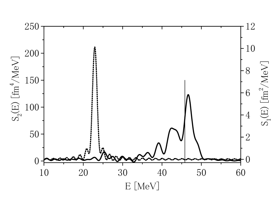
FIG. 1.: Strength function $S_{2}(E)$ of the DGDR in ¹⁶O calculated in TDDM (thick solid line). The dotted line denotes the strength function $S_{1}(E)$ of the GDR in RPA and the thin vertical bar at $E=45.8$MeV indicates the location of the DGDR predicted from the GDR in RPA (in arbitrary units).

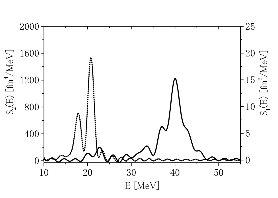
FIG. 2.: Strength function $S_{2}(E)$ of the DGDR in ⁴⁰Ca calculated in TDDM (solid line). The dotted line denotes the strength function $S_{1}(E)$ of the GDR in RPA.

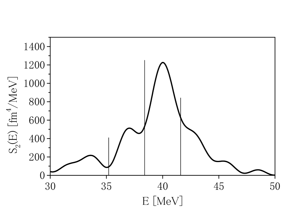
FIG. 3.: Strength function $S_{2}(E)$ of the DGDR in ⁴⁰Ca calculated in TDDM (thick solid line) is compared with what is predicted from the strength function of the GDR shown in Fig.2 (thin vertical bars in arbitrary units).

REFERENCES

- [1] P. Chomaz and N. Frascaria, Phys. Rep. 252 (1995) 275; T. Aumann, P. F. Bortignon, H. Emling, Ann. Rev. Nucl. Part. Sci. 48 (1998) and references therein.
- [2] C. A. Bertulani and V. Y. Ponomarev, Phys. Rep. 321 (1999) 139.
- [3] S. Nishizaki and J. Wambach, Phys. Lett. B 349 (1995) 7.
- [4] S. Nishizaki and J. Wambach, Phys. Rev. C57 (1998) 1515.
- [5] N. D. Dang, K. Tanabe and A. Arima, Phys. Rev. C59 (1999) 3128.
- [6] G. Bertsch and S. Tsai, Phys. Rep. C18 (1975) 125.
- [7] M. Tohyama, Prog. Theor. Phys. 100 (1998) 1293.
- [8] M. Gong and M. Tohyama, Z. Phys. A335 (1990) 153.
- [9] M. Tohyama, Nucl. Phys. A657 (1999) 343.
- [10] S. J. Wang and W. Cassing, Ann. Phys. 159 (1985) 328; W. Cassing and S. J. Wang, Z. Phys. 328 (1987) 423.
- [11] M. Tohyama and M. Gong, Z. Phys. A332 (1989) 269.
- [12] J. Sawicki, Phys. Rev. 126 (1962) 2231; J. Da Providencia, Nucl. Phys. 61 (1965) 87.
- [13] C. Yannouleas, Phys. Rev. C35 (1987) 1159.
- [14] S. Drod et al., Phys. Rep. 197 (1990) 1.
- [15] D. Vautherin and D. M. Brink, Phys. Rev. C5 (1972) 626.
- [16] M. Beiner, H. Flocard, Nguyen van Giai, and P. Quentin, Nucl. Phys. A238 (1975) 29.
- [17] M. Tohyama, Prog. Theor. Phys. 99 (1998) 109.
- [18] M. Tohyama, Phys. Lett. B323 (1994) 257.
- [19] F. F. de Souza Cruz and L. I. Weiss, J. Phys. G21 (1995) 43.
- [20] G. F. Bertsch and H. Feldmeier, Phys. Rev. C56 (1997) 839.
- [21] F. Catara, Ph. Chomaz and N. Van Giai, Phys. Lett. B233 (1989) 6.
- [22] E. G. Lanza et al., Nucl. Phys. A636 (1998) 452.