Vacuum structure in QCD and Correlation functions

Abstract

We discuss here a model of QCD vacuum in terms of quark antiquark and gluon condensates alongwith their fluctuations. The correlation functions of hadronic currents in such a vacuum are evaluated to extract hadron properties. The presence of fluctuations of the condensates are emphasized. The structure of vacuum is then generalised to finite temperatures to study correlation functions at finite temperatures. Finally, we discuss the vacuum structure at finite densities with diquark condensates in a Nambu JonaLasinio type model. The coupled mass gap and superconducting gap equations are solved selfconsistently. For certain parameters of the model nontrivial solutions of both the gap equations are obtained. The equation of state is also computed.

PACS number(s): 12.38.Gc

I Introduction

Quantum chromodynamics (QCD) is now accepted to be the theory of strong interaction in terms of quarks and gluons, and, at a secondary level, of hadrons. It is a nonabelian gauge theory with $SU(3)$ as the gauge group. This nonabelianess of the interaction leads to two important consequences. Firstly, the interaction become weak at high momentum (above several GeV) transfer processes where perturbation theory is applicable. At low energies and momenta, relevant to most of nuclear physics, the quark gluon coupling strength becomes large and an expansion in powers of this coupling is not useful. The basic difficulty appears to be an understanding of the ground state properties of QCD or its vacuum structure which plays an important role for the related physics [1].

Conceptually, low energy QCD has many common feature with condensed matter physics. The vacuum here appear to be consisting of having fluctuating quarks and gluon fields with average properties being described by condensates of quarks and gluons. The quark condensate $\langle\bar{q}q\rangle$, i.e. expectation value of quark scalar densities, plays an important role in the context of strong interactions. It displays the breaking of chiral symmetry. This symmetry is crucial to our understanding of nucleons,nuclei and dense matter. The other quantity that charcterise the QCD vacuum is the gluon condensate. The energy density of vacuum is lowered by presence of electric and magnetic gluon fields in the ground state. These condensates were introduced in the context of QCD sumrules and the values are estimated from the charmonia spectroscopy as $\langle\alpha_{s}/\pi GG\rangle=\langle 2\alpha_{s}/\pi^{2}({\bf{E}}^{2}-{\bf{B}}^{2})\rangle=0.012GeV^{4}$ and $\langle\bar{q}q\rangle=-(250MeV)^{3}$ [2].

Thus QCD vacuum poses a rich complicated many body problem. As in other many body system ground state correlation functions give an insight to the ground state structure. One might be interested in asking questions like what happens to a meson pair when placed in such a condensate medium or what happens to interquark interaction as a function of their spatial separation. We might remind ourselves that nucleon scattering phase shifts gives information regading inter-nucleon forces complementary to that infered from their bound state namely from the properties of deuteron. N-N scattering allows one to study different components of nuclear forces (spin-spin, tensor,$\cdots$) at different spatial separation in much more detail than deuteron observables which is an composite effects of all channels. In QCD we however do not have free quarks or gluons due to confinement. None the less, one can infer about inter-quark interaction as a function of their separation in different channels by studying propagators and correlation functions of hadron currents in a more detailed manner than the composite effects reflected in hadron bound state. The correlation functions that we shall consider here are spacelike separated correlation functions. To be precise we shall take the correlation functions to be defined at equal time so that their separation is purely spatial. Such correlation functions have several appealing features. They describe different physics at different spatial separations; they can be calculated in some channels phenomenologically from $e^{+}e^{-}\rightarrow$hadrons data or from $\tau$ decay experimental data. Moreover they can be evaluated in lattice simulations [3] or in some model for vacuum[4].

Our appraoch here shall be assuming a structure for the vacuum and then examining its consequences regarding correlator phenomenology. More precisely, we shall use phenomenological results of correlation functions of hadronic currents [3] to guide us towards a “true” structure of QCD vacuum. We organise this note as follows. In section II, we shall discuss a construct for the vacuum in terms of quark and gluon condensates [5], and the resulting correlation functions [6]. It appears that condensates alone do not give rise to correct phenomenology of correlators unless one includes fluctuations of such condensates [7]. Inclusion of the fluctuation fields yields correlation functions consistent with the phenomenology of correlation functions. Such a structure of vacuum of zero temeperature is then generalised to finite temperature in section III. Here we shall also compute the finite temperature correlators to determine temperature dependent hadron properties [8]. In section IV, we shall discuss the vacuum structure at high density and the QCD vacuum with diquark condensate giving rise to color superconductivity. Finally, we summarize our results with some remarks and discussions in section V.

II An ansatz for the QCD vacuum and correlation functions

A variational ansatz was considered in Ref.[5] for the QCD vacuum with an explicit construct involving quark antiquark pairs and gluon pairs. The trial ansatz was given as

$$|vac\rangle=\exp(B_{F}^{\dagger}-B_{F})(B_{G}^{\dagger}-B_{G})|0\rangle$$ (1)

where, the Bogoliubov pair creation operators for the quarks and the gluons are given respectively as

$$B_{F}^{\dagger}=\int q_{I}^{0}({\bf{k}})^{\dagger}(\mbox{\boldmath$\sigma$}\cdot{\bf{k}})h({\bf{k}})\tilde{q}_{I}^{0}({\bf{k}})d{\bf{k}},$$ (3)

and,

$$B_{G}^{\dagger}=\int a_{i}^{a}({\bf{k}})^{\dagger}g({\bf{k}})a_{i}^{a}(-{\bf{k}})d{\bf{k}}.$$ (4)

In the above $q^{0}_{I},\tilde{q}^{\dagger 0}_{I}$ are two component quark and antiquark annihilation operators respectively. The subscript $0$ indicates that they annihilate the peruturbative vacuum $|0\rangle$ i.e. $q_{I}^{0}|0\rangle=0=\tilde{q}^{\dagger}|0\rangle$. $a_{i}^{a}$ is the gluon annihilation operator. The operators satisfy the quantum algebra given in Coulomb gauge as

$$\left[q^{i0}_{Ir}({\bf{k}}),q^{0j}_{Is}({\bf{k}}^{\prime})^{\dagger}\right]_{+}=\delta^{ij}\delta_{rs}\delta({\bf{k}}-{\bf{k}}^{\prime}),$$ (6)

and,

$$\left[a_{i}^{a}({\bf{k}}),a_{j}^{b}({\bf{k}}^{\prime})\right]=\delta^{ab}\left(\delta_{ij}-{\bf{k}}_{i}{\bf{k}}_{j}/{\bf{k}}^{2}\right)\delta({\bf{k}}-{\bf{k}}^{\prime}).$$ (7)

Finally, $h({\bf{k}})$ and $g({\bf{k}})$ are two trial functions associated with the quark antiquark condensates and gluon pairs respectively. Clearly, a construct as in Eq.(1)has an obvious parallel to BCS theory of superconductivity. Such a structure for vacuum eventually reduces to Bogoliubov transformation for the operators. Then one can calculate the, energy functional–the expectation value of the Hamiltonian which is a functional of the condensate functions. Since the functions cannot be determined through functional minimisations one can parametrise the condensate functions with some trial functions simple enough to manipulate numerically as well as reasonable enough to simulate correct physical behaviour. In Ref.[5], the following choices were made (with $k=|{\bf{k}}|$)

$$\tan 2h({\bf{k}})=\frac{A^{\prime}}{(\exp(R^{2}k^{2})-1)^{1/2}}$$ (9)

$$\sinh g({\bf{k}})=A\exp(-bk^{2})$$ (10)

In Ref.[5] the energy density was minimised with respect to the condensate parameters subjected to the constraint that the pion decay constant $f_{\pi}$ and the gluon condensate value $(\alpha_{s}/\pi)\langle GG\rangle$ turns out to be the experimental values of 93 MeV and $0.012GeV^{4}$ respectively. The result of such a minimisation then leads to instabilty of perturbative vacuum to condensate formation beyond a critical coupling of $\alpha_{s}^{c}=0.6$. For $\alpha_{s}=1.28$, the charge radius of pion comes out correctly. The values of $A^{\prime}$ and $R$ turns out to be $A^{\prime}\simeq 1$ and $R\simeq 0.96fm.$ Further some of the baryonic properties like charge radius of proton, magnetic moments of proton and neutron turns out to be close to their corresponding experimental values. Further, the bag constant– the energy difference between the perturbative and the nonperturbative vacuum turns out to be $\epsilon_{0}=-(140MeV)^{4}$which appears to be in general agreement with the phenomenological value of this parameter.

With such a description of the vacuum in terms of condensates let us look at the correlation functions and propagators in a condensed medium. The equal time propagator is given as[9]

$$S_{\alpha\beta}({\bf{x}}) = \langle\frac{1}{2}\left[q_{\alpha}({\bf{x}}),\bar{q}_{\beta}({\bf{0}})\right]\rangle$$ (11)

$$= \frac{1}{2}\frac{1}{(2\pi)^{3}}\int e^{i{\bf{k}}\cdot{\bf{x}}}\left[\sin 2h({\bf{k}})-\mbox{\boldmath$\gamma$}\cdot{\bf{k}}\cos 2h({\bf{k}})\right]$$ (12)

Clearly, free massless propagator corresponds to $h({\bf{k}})\rightarrow 0$ limit of above equation and is given as $S_{0}=-(i/2\pi^{2})(\mbox{\boldmath$\gamma$}\cdot{\bf{x}}/x^{4})$. Different components of the propagator given in Eq.(LABEL:prop) can be analysed[6] and it turns out to be qualitatively similar to those obtained from other nonperturbative calculations like an instanton liquid model for QCD vacuum[4, 10]. Further, a small x expansion of Eq.(LABEL:prop) yields the propagtor as that one would get in the operator product expansion in the vacuum saturation approximation[10].

We shall next consider the correlation functions of mesonic currents of generic form $J({\bf{x}})=\bar{q}_{\alpha}({\bf{x}})\Gamma_{\alpha\beta}q_{\beta}({\bf{x}})$, where $\alpha,\beta$ are spinor indices and $\Gamma$ is a 4$\times$4 matrix in Dirac space $(1,\gamma_{5},\gamma_{\mu},\gamma_{\mu}\gamma_{5})$. The equal time correlation function is defined as

$$R({\bf{x}})=\frac{1}{2}\langle vac|J({\bf{x}})\bar{J}({\bf{0}})|vac\rangle+\langle vac|\bar{J}({\bf{0}})J({\bf{x}})|vac\rangle$$ (14)

With the definition of condensate vacuum as in Eq.(1) and the propagator given in Eq.(LABEL:prop), Eq.(14) reduces to

$$R(x)=-Tr[S(x)\Gamma^{\prime}S(-x)\Gamma]$$ (15)

where, $\Gamma^{\prime}=\gamma_{0}\Gamma^{\dagger}\gamma_{0}$. We shall be normalising the correlation functions with that of free massless correlation function which is given as parallel to Eq(15) as

$$R_{0}(x)=-Tr[S_{0}(x)\Gamma^{\prime}S_{0}(-x)\Gamma]$$ (16)

The ratio $R(x)/R_{0}(x)$ can then be evaluated for different channels. It turns out that correlation function so obtained has similar qualitative behaviour as one can obtain from phenomenology in all chnnels except for the pseudoscalar channel [6]. Phenomenologically, in this channel there is a strong attraction with the ratio becoming about 100 at a separation of about a fermi[4]. The calculated value however turns out to be as low as 1.2 around that value. All these results depend very weakly on the functional form of $h({\bf{k}})$.

In view of this outcome, it is obvious that some crucial physics is missing from the model of vacuum considered in Eq.(1) and has to be supplemented by additional effects. In the present framework this means that quark propagators alone do not describe the correlation functions and there has to be contributions from irreducible four point structure of the vacuum. This can be thought of as a manifestation of fluctuation of the condensates. Thus we have

$$T\bar{q}_{\alpha}({\bf{x}})q_{\beta}({\bf{x}})q_{\gamma}({\bf{0}})q_{\delta}({\bf{0}}) = S_{\beta\gamma}({\bf{x}})S_{\delta\alpha}(-{\bf{x}})+:\bar{q}_{\alpha}({\bf{x}})q_{\beta}({\bf{x}})q_{\gamma}({\bf{0}})q_{\delta}({\bf{0}}):$$ (17)

$$= S_{\beta\gamma}({\bf{x}})S_{\delta\alpha}(-{\bf{x}})+\Sigma_{\beta\gamma}({\bf{x}})\Sigma_{\delta\alpha}(-zbfx)$$ (18)

where, we have introduced the composite fields $\Sigma$ to include the effects of fluctuation with $\langle vac|\Sigma\Sigma|vac\rangle=0$ but $\langle\Omega|\Sigma\Sigma|\Omega\rangle\neq 0$, where, $|\Omega\rangle$is the “new improved” QCD vacuum including the condensate fluctuations. The correlation function then takes the form

$$R(x)=-\left[Tr[S(x)\Gamma^{\prime}S(-x)\Gamma]+Tr\left[\Sigma({\bf{x}}))\Gamma^{\prime}\Sigma(-x)\Gamma\right]\right]$$ (20)

The structure of $\Sigma$ field should be such that it contributes mostly to the pseudoscalar channel and should not affect the other channels very much. Such a condition restricts the composite field to be of the form

$$\Sigma_{\alpha\beta}({\bf{x}})=\mu_{1}^{2}(\gamma^{i}\gamma^{j}\epsilon_{ijk}\phi^{k}({\bf{x}})+\mu_{2}^{2}\delta_{\alpha\beta}\phi({\bf{x}})$$ (21)

where, we have introduced the scalar and vector fileds $\phi$ and $\phi^{k}$ such that

$$\langle\Omega|\phi^{i}({\bf{x}})\phi^{j}({\bf{0}})|\Omega\rangle=\delta^{ij}g_{V}({\bf{x}})$$ (23)

$$\langle\Omega|\phi({\bf{x}})\phi({\bf{0}})|\Omega\rangle=g_{S}({\bf{x}})$$ (24)

From general considerations, we may write down the functions $g_{V}({\bf{x}}),g_{S}({\bf{x}})$ as[7]

$$g_{V}({\bf{x}})=\frac{1}{2\pi^{2}x}\left[\mu_{1}K_{1}(\mu_{1}x)-\mu_{3}K_{1}(\mu_{3}x)\right]$$ (26)

$$g_{S}({\bf{x}})=\frac{1}{2\pi^{2}x}\left[\mu_{2}K_{1}(\mu_{4}x)-\mu_{5}K_{1}(\mu_{6}x)\right]$$ (27)

Using Eq.s(20,21,26,27) one can have the expression for the correlation functions in different channels. Explicitly different currents in different channels and the contributions from the propagator and the fluctuation fields are shown separately in Table I. We have also included here the currents for the baryons. The resulting correlation functions normalised to correlation functions obtained by treating the quarks as massless and noninteracting are plotted in Fig.1.

FIG. 1.: The ratio of hadron correlation functions in QCD vacuum to the correlation functions for noninteracting massless quarks $R(x)/R_{0}(x)$ , vs distance x (in fermi). Our results are given by the solid curves. The emperical results determined from dispersion analysis of experimantal data in Ref. are shown by long dashed lines. The results from lattice calculations and instanton liquid model are denoted by dotted and dot-dashed lines respectively.

TABLE I.: Meson currents and correlation functions

CHANNEL	CURRENT	CORRELATION FUNCTIONS $\displaystyle\left[\;\frac{R(x)}{R_{0}(x)}\;\right]$
		Without fluctuationsa	Fluctuation contribution
			(Vector($F^{V}$) and Scalar ($F^{S}$))
Vector	$\bar{u}\gamma_{\mu}d$	$[F(x)]^{2}+\frac{\pi}{4}\frac{x^{6}}{R^{6}}e^{-x^{2}/R^{2}}$	$F^{V}=0$
			$F^{S}=8\pi^{4}x^{6}g_{S}(2x)$
Pseudoscalar	$\bar{u}\gamma_{5}d$	$[F(x)]^{2}+\frac{\pi}{8}\frac{x^{6}}{R^{6}}e^{-x^{2}/R^{2}}$	$F^{V}=-48\pi^{4}x^{6}g_{V}(2x)$
			$F^{S}=4\pi^{4}x^{6}g_{S}(2x)$
Nucleon	$\epsilon_{abc}\left[\tilde{u}^{a}(x)C\gamma_{\mu}u^{b}(x)\right]\gamma^{\mu}\gamma_{5}d^{c}(x)$	$[F(x)]^{3}+\frac{\pi}{16}\frac{x^{6}}{R^{6}}e^{-x^{2}/R^{2}}F(x)$	$F^{V}=-4\pi^{4}x^{6}g_{V}(2x)F(x)$
			$F^{S}=2\pi^{4}x^{6}g_{S}(2x)F(x)$
Delta	$\epsilon_{abc}\left[\tilde{u}^{a}(x)C\gamma_{\mu}u^{b}(x)\right]u^{c}(x)$	$[F(x)]^{3}+\frac{\pi}{4}\frac{x^{6}}{R^{6}}e^{-x^{2}/R^{2}}F(x)$	$F^{V}=0$
			$F^{S}=8\pi^{4}x^{6}g_{S}(2x)F(x)$

To get the hadron parameters from the correlation functions one relates the correlation function through a dispersion relation to a spectral density function. For example in the vector channel the dispersion relation for the correlation function reduces to [4]

$$\Pi_{\mu\mu}(x)\equiv\langle\Omega|T(J_{\mu}(x)\bar{J}_{\mu}(0))|\Omega\rangle=\frac{1}{4\pi^{2}}\int_{0}^{\infty}dsR_{i}(s)D(s^{1/2},x)$$ (28)

with, the function $D(m,x)=(m/4\pi^{2}x)K_{1}(mx)$ is a propagator of a particle of mass $m$. The function $R_{i}(x)$ is the normalised spectral density function related to the cross section of $e^{+}e^{-}$ annihilation to hadrons. In presence of interaction, in general we do not know how to calculate the spectral density function . However we do know their qualitative behaviour based on experimental information. To extract hadron parameters one parametrises the spectral function and then determine the parameters. A useful parametrisation valid at zero temperature is in terms of a Dirac delta function at the pole mass of the hadron accompanied by a step function continuum at higher energy. Specifically, for $\rho$ meson the spectral density function is parametrised by

$$R_{\rho}(s)=3\lambda^{2}\delta(s-M^{2})+\frac{3s}{4\pi^{2}}\theta(s-s_{0}).$$ (29)

TABLE II.: Fitted Parameters

CHANNEL	SOURCE	M (GeV)	$\lambda$	$\sqrt{s_{0}}$(GeV)
Vector	Ours	0.78 $\pm$ 0.005	(0.42 $\pm$ 0.041 GeV)2	2.07 $\pm$ 0.02
	Lattice	0.72 $\pm$ 0.06	(0.41 $\pm$ 0.02 GeV)2	1.62 $\pm$ 0.23
	Instanton	0.95 $\pm$ 0.10	(0.39 $\pm$ 0.02 GeV)2	1.50 $\pm$ 0.10
	Phenomenology	0.78	(0.409 $\pm$ 0.005 GeV)2	1.59 $\pm$ 0.02
Pseudoscalar	Ours	0.137 $\pm$ 0.0001	(0.475 $\pm$ 0.015 GeV)2	2.12 $\pm$ 0.083
	Lattice	0.156 $\pm$ 0.01	(0.44 $\pm$ 0.01 GeV)2	$\;\;\;<$ 1.0
	Instanton	0.142 $\pm$ 0.014	(0.51 $\pm$ 0.02 GeV)2	1.36 $\pm$ 0.10
	Phenomenology	0.138	(0.480 GeV)2	1.30 $\pm$ 0.10
Nucleon	Ours	0.87 $\pm$ 0.005	(0.286 $\pm$ 0.041 GeV)3	1.91 $\pm$ 0.02
	Lattice	0.95 $\pm$ 0.05	(0.293 $\pm$ 0.015 GeV)3	$\;\;\;<$ 1.4
	Instanton	0.96 $\pm$ 0.03	(0.317 $\pm$ 0.004 GeV)3	1.92 $\pm$ 0.05
	Sum rule	1.02 $\pm$ 0.12	(0.337 $\pm$ 0.0.014 GeV)3	1.5
	Phenomenology	0.939	$\;\;\;?$	1.44 $\pm$ 0.04
Delta	Ours	1.52 $\pm$ 0.003	(0.341 $\pm$ 0.041 GeV)3	3.10 $\pm$ 0.008
	Lattice	1.43 $\pm$ 0.08	(0.326 $\pm$ 0.020 GeV)3	3.21 $\pm$ 0.34
	Instanton	1.44 $\pm$ 0.07	(0.321 $\pm$ 0.016 GeV)3	1.96 $\pm$ 0.10
	Sum rule	1.37 $\pm$ 0.12	(0.337 $\pm$ 0.014 GeV)3	2.1
	Phenomenology	1.232	$\>\;\;?$	1.96 $\pm$ 0.10

where, M is the bound state mass, $\lambda$ is the coupling of the current to the bound state and $s_{0}$ is the threshold for continuum contribution. The fitted parametrs to the correlation functions obatined by us (solid curve in Fig.1 are given in Table II

As may be evident from this the results are comparable with that of lattice calculation [3] and instanton liquid model calculations [4]. Thus to be consistent with the data QCD vacuum must not only have condensates but also have their fluctuations.

III QCD vacuum and correlation functions at finite temperature

As is well known [11] the QCD vacuum state changes with temperature. Lattice Monte Carlo simulations suggest that chiral symmetry is restored around 150 MeV. Thus it is interesting to look at correlation functions at finite temperature in the context of behaviour of hadrons around the chiral phase transition [12, 13]. It may be noted that there is little phenomenological information in this regime but there are several theoretical studies [14, 15, 16, 17] using operator product expansion (OPE) and sum rule methods as well as using instanton liquid model for QCD ground state [18, 19]. In particular, we shall generalise the method considerd in the previous section to include temperature effects. The zero temperature vacuum defined in Eq.(1) can be generalised to finite temperature using the methodology of thermofield dynamics. Here the thermal average of an operator is obtained as an expectation value of the operator over the thermal vacuum[20]. The thermal vacuum is obtained from the zero temperature vacuum by a thermal Bogoliubov transformation in an extended Hilbert space involving extra field operators (thermal doubling of operators)[20]. Explicitly, the thermal vacuum is given as

$$|vac,\beta\rangle=\exp\left(\int d{\bf{k}}\theta({{\bf{k}},\beta})({q_{I}}^{\dagger}({\bf{k}})\underline{q_{I}}^{\dagger}(-{\bf{k}})+{\tilde{q}}_{I}({\bf{k}})\underline{\tilde{q}}_{I}(-{\bf{k}}))-h.c.\right)|vac\rangle$$ (30)

where, the underlined oprators are the operators corresponding to extra of Hilbert space. Further, the $q_{I}^{\prime}s$ are the opeartors refers to the fact that they are the quasi paricle operators corresponding to basis defined by the vacuum of Eq.(1) i.e. $q_{I}|vac\rangle=0=\tilde{q}^{\dagger}_{I}|vac\rangle$ and finally $\theta(k,\beta)$ is the function for the thermal Bogoliubov transformation and is related to the number density function given as

$$\sin^{2}\theta({\bf{k}},\beta)=\frac{1}{\exp(\beta\epsilon)+1}$$ (31)

where, $\epsilon({\bf{k}})$ is the single particle energy given as $\epsilon({\bf{k}})=\sqrt{{\bf{k}}^{2}+m(k)^{2}}$. In the presence of condensate the dynamical mass is given as $m(k)=k\tan 2h(k)$ [5]. As before the equal time propagator can be calculated including the temperature effects as

$$S_{\alpha\beta}({\bf{x}}) = \langle vac,\beta|\frac{1}{2}\left[q_{\alpha}({\bf{x}}),\bar{q}_{\beta}({\bf{0}})\right]|vac,\beta\rangle$$ (32)

$$= \frac{1}{2}\frac{1}{(2\pi)^{3}}\int e^{i{\bf{k}}\cdot{\bf{x}}}\cos\!2\theta({\bf{k}},\beta)\left[\sin 2h({\bf{k}})-{\bf{\gamma}}\cdot{\bf{k}}\cos 2h({\bf{k}})\right]$$ (33)

As in Section III, we shall take a gaussian ansatz for the condensate function $\sin 2h({\bf{k}})=\exp(-R(T)^{2}{\bf{k}}^{2}/2$, with the condensate scale parameter $R$, now being temperature dependent. In order to determine $R(T)$ or equivalently the ratio $S(T)=R(T=0)/R(T)$, we first evaluate our expression of the order parameter (the condensate value) at finite temperature. In terms of the dimensionless variable $\eta=Rk$, this is given as

$$\frac{\langle\bar{q}q\rangle_{T}}{\langle\bar{q}q\rangle_{T=0}}=S(T)^{3}\bigg{[}1-2\sqrt{\frac{2}{\pi}}\int e^{-\eta^{2}/2}\sin^{2}(z,\eta)\eta^{2}d\eta\bigg{]},$$ (35)

where $\sin^{2}\theta(z,\eta)={1}/\left(\exp(z\epsilon(\eta))+1)\right)$, with $z=\beta/R(T)$ and $\epsilon(\eta)=\eta/\cos 2h(\eta)$.

We can obtain $S(T)=R(T=0)/R(T)$ if we know the temperature dependence of the order parameter on the left hand side of Eq.(35). As there are no phenomenological inputs for this, we shall proceed in the following manner to take the temperature dependence of the quark condensate. For low temperatures we shall take the results from chiral perturbation theory (CHPT) which is expected to be valid at least for small temperatures[22]. For higher temperatures near the critical temperature, lattice simulations seem to yield the universal behaviour[11] with a large correlation length associated with a second order phase transition for two flavor massless QCD. We shall use such a critical behaviour to consider the temperature dependence of the order parameter near the critical temperature.

FIG. 2.: Figure (a) shows quark condensate at finite temperature normalised to that at zero temperature obtained from CHPT and Lattice. Figure (b) shows R(0)/R(T) as determined from Fig (a).

For intermediate regime we shall take a smooth interpolation between the two. The resulting behaviour of the temperature dependance of the quark condensate and the ratio $R(0)/R(T)$ determined using Eq.(35) are shown in Fig.s 2.

With the temperature dependence of $R(T)$ known as above, the propagator function of eq.(LABEL:propt) now completely defined. The finite temperature correlation function is now given as, parallel to Eq.(20)

$$R({\bf{x}},T)=-\left[Tr[S({\bf{x}},T)\Gamma^{\prime}S(-{\bf{x}},T)\Gamma]+Tr\langle\left[\Sigma({\bf{x}}))\Gamma^{\prime}\Sigma(-{\bf{x}})\Gamma\right]\right]\rangle_{T}.$$ (36)

The second term in the above corresponds to contributions from the fluctuations at finite temperature that can be written interms of the functions $g_{S}({\bf{x}},T),g_{V}({\bf{x}},T)$ as earlier but now being temperature dependent. We do not know how to calculate it except for a general property that the effect of the four point structure should decrease with temperature. We take here a simple ansatz for the temperature dependence of $g_{V}$ and $g_{S}$,

$$g_{S,V}({\bf{x}},T)=\left(\frac{\langle\bar{q}q\rangle_{T}}{\langle\bar{q}q\rangle_{T=0}}\right)^{2}\;\;g_{S,V}({\bf{x}},T=0)$$ (37)

The parameters $\mu_{i}$ are choosen to have the same values as of zero temperature while fitting the mesonic and baryonic correlation function. The normalised correlation functions $R({\bf{x}},T)/R_{0}({\bf{x}},T=0)$ are plotted in Fig.4a and Fig 4b respectively.

As expected (on physical grounds) the amplitude of the correlator decreases with increasing temperature. The peak of the vector correlator shifts towards the right after $T=0.9T_{c}$. We might remind ourselves that the position of the peak of the correlator is inversely proportional to the mass of the particle in the relevant channel[3].

To extract hadronic properties at finite temperature, the correlators are parametrised in terms of a spectral density function. This is a generalisation of eq.(29) to finite temperature and is given as [15, 17],

$$\rho^{V}(s)=3\lambda_{\rho}^{2}\delta(s-M_{\rho}^{2})+\frac{3s}{4\pi^{2}}\tanh\left[\frac{\sqrt{s}}{4T}\right]\theta(s-s_{o})+T^{2}{S_{\rho}}\delta(s)$$ (38)

$$\rho^{P}(s)=\lambda_{\pi}^{2}\delta(s-M_{\pi}^{2})+\frac{3s}{8\pi^{2}}\tanh\left[\frac{\sqrt{s}}{4T}\right]\theta(s-s_{o})$$ (39)

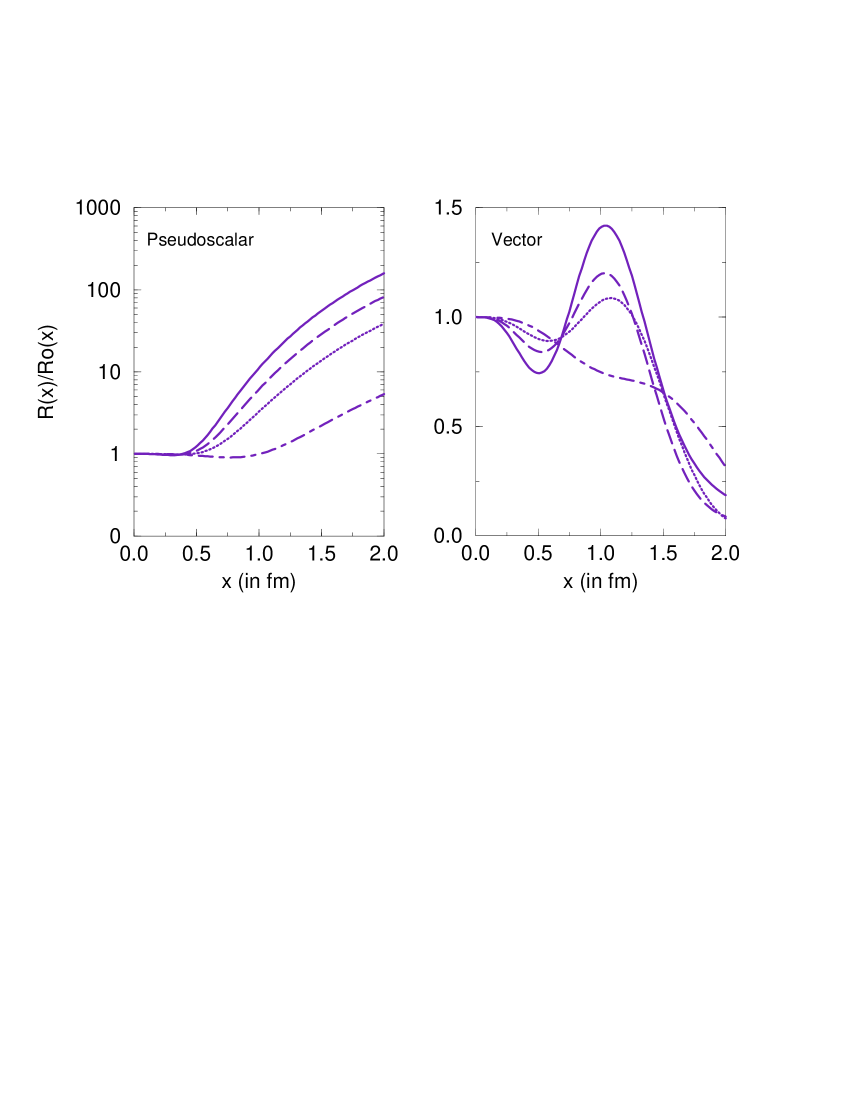
FIG. 3.: The ratio of the meson correlation functions at finite temperature to the correlation functions for noninteracting massless quarks at zero temperature $\em{R(x,T)}/{R_{0}(x,T=0)}$, vs. distance x (in fm). The solid, dashed, dotted and dot-dashed lines correspond to temperatures $T=$0 MeV, $T=$130 MeV, $T=$140 MeV and $T=$148 MeV respectively.

Eq.(39) corresponds to spectral density function for pseudoscalar channel. The last term in Eq.(38) The last term in Eq. (38) is the scattering term for soft thermal dissociations (mainly through pions), which exists only at finite temperature[15] and can be taken as  [15]$S_{\rho}\approx\frac{T^{2}}{9}$.

The mass, threshold and coupling are then extracted and the results are plotted in Fig. 4 for the vector and in the pseudoscalar channel. As can be seen from Fig.s3, with increase in temperature, the correlation functions have a lower peak indicating lack of correlations with temperature. In the vector channel the mass of the $\rho$ meson appears to decrease for temperatures beyond 120 MeV. The threshold for the continuum also decreases around the same temperature. The behaviour with temperature of these quantities is qualitatively similar to that found by Hatsuda et al[17]. We have also plotted the temperature dependence of the coupling of the bound state to the current which decreases with temperature but rather slowly as compared to mass or the threshold for the continuum. The temperature dependence of these parameters can be used to calculate the lepton pair production rate from $\rho$ in the context of ultra relativistic heavy ion collision experiments to estimate vector meson mass shift in the medium.

In the pseudoscalar channel the mass remains almost constant till the critical temperature whereas the thershold and the coupling decrase with the temparature. We have found that in the pseudoscalar channel, the contribution to the correlation function mostly comes from the fluctuating fields. Further, the temperature behaviour as taken in Eq.(37) essentially does not shift the position of the peak whereas the magnitude of the correlator decreases. That is reflected in the above behaviour of the parameters in the pseudoscalar channel. We may note here that similar behaviour of pion mass becoming almost insensitive to temperature below the critical temperature was also observed in Ref.[23] where correlation functions were calculated in a QCD motivated effective theory namely the Nambu- Jona Lasinio model.

,

FIG. 4.: The temperature dependence of mass, threshold (S₀) and coupling for the vector (left panel) and pseudoscalar (right panel) channel. T${}_{c}=$150 MeV. The vertical lines represent the errors obtained while fitting.

IV QCD vacuum at finite densities

Let us now go over to explore the ground state structure in high density QCD. Unlike high temperatures, rather little is known about QCD at finite baryon densities from first principles like lattice QCD simulation due to technical problems. However, different low energy models of QCD seem to indicate a rich phase structure in this domain. In particular the color superconductivity phase at high density has attracted much attention. Although it was known for quite sometime [24], recent studies [25, 26, 27, 28] indicated that the superconducting gap could be as large as 100 MeV and that has lead to an extensive literature on this subject in recent past regarding its consequences in neutron stars as well as for heavy ion collisions.

As per BCS theorem, an arbitrarily weak attractive interaction makes the fermi sea of quarks unsatble at high densities. In deed, the color current current interaction is attractive in the scalar $(\bar{\mbox{\boldmath$3$}})$ and axial vector channel. This can lead to formation of Cooper pairs and associated superconductivity in the color space. To discuss it in a nonperturbative manner, we take the trial ansatz over the chiral condensed vacuum of Eq.(1) as [29]

$$|\omega\rangle=\exp\left[\frac{1}{2}\int\left[q_{r}^{ia}({\bf{k}})^{\dagger}f({\bf{k}})q_{-r}^{jb}(-{\bf{k}})^{\dagger}\epsilon_{ij}\epsilon_{3ab}+\tilde{q}_{r}^{ia}({\bf{k}})f_{1}({\bf{k}})\tilde{q}_{-r}^{jb}(-{\bf{k}})\epsilon_{ij}\epsilon_{3ab}\right]d{\bf{k}}.\right]|vac\rangle$$ (40)

In the above, $i,j$ are flavor indices, $a,b$ are the color indices and $r(=\pm 1/2)$ is the spin index. We shall consider here two flavor and SU(3) color. Here we have also introduced two trial functions $f({\bf{k}})$ and $f_{1}({\bf{k}})$ respectively for the diquark and diantiquark channel. As may be noted the state constructed in Eq.(40) is spin singlet and is antisymmetric in color and flavor.

Next, to include the effect of temperature and density, we obtain the state at finite temperature and density $|\omega(\beta,\mu)\rangle$ by a thermal Bogoliubov transformation over the state $|\omega\rangle$ using thermofield dynamics as in Eq.(30)[8, 20, 21, 38],

$$|\omega(\beta,\mu)\rangle=\exp\left(\int q_{I}({\bf{k}})^{\dagger}\theta_{-}({\bf{k}},\beta,\mu)\underline{q}_{I}({\bf{k}})^{\dagger}+\tilde{q}_{I}({\bf{k}})\theta_{+}({\bf{k}},\beta,\mu)\underline{\tilde{q}}_{I}({\bf{k}})d{\bf{k}}-h.c.\right)|\omega\rangle$$ (41)

In the above, the ansatz functions $\theta_{\pm}({\bf{k}},\beta,\mu)$, as before, will be related to quark and antiquark distributions. We might note here that the trial ansatz given in Eq.(41) actually invloves five functions - $h({\bf{k}})$, for the quark anti quark condensates, $f({\bf{k}})$ and $f_{1}({\bf{k}})$ describing respectively the diquark and diantiquark condensates and $\theta_{\pm}({\bf{k}},\beta,\mu)$ to include the temperature and density effects. All these functions are to be obtained by minimising the thermodynamic potential. This will involve an assumption about the effective hamiltonian . For the purpose of illustration we shall consider a hamiltonian of Nambu-Jonalasinio type given as

$${\cal H}=\psi^{\dagger}(-i\mbox{\boldmath$\alpha$}\cdot\mbox{\boldmath$\nabla$})\psi+\frac{g^{2}}{2}J_{\mu}^{a}J^{\mu a}.$$ (42)

with $J_{\mu}^{a}=\bar{q}\gamma^{\mu}T^{a}q$. One can then calculate the energy functional $\epsilon=\langle\omega(\beta,\mu)|{\cal H}|\omega(\beta,\mu)\rangle$ and the thermodynamic potential ${\cal F}=\epsilon-(1/\beta)S-\mu N$, using the Bogoliubov technique. The details are given in Ref. [29]. The free energy is a functional of all the five functions $h,f,f_{1},\theta_{\pm}$. However with the point interaction of the the Hamiltonian of eq.(42) one can determine them. This results in two coupled gap equations to be solved in a self consistent manner and are given as

$$\frac{4g^{2}}{3}\frac{1}{(2\pi)^{3}}\int d{\bf{k}}\frac{1}{\sqrt{{\bf{k}}^{2}+M^{2}}}\left(\frac{\xi_{-}}{\omega_{-}}tanh(\frac{\beta\omega_{-}}{2})+\frac{\xi_{+}}{\omega_{+}}tanh(\frac{\beta\omega_{+}}{2})\right)=1$$ (44)

$$\frac{4g^{2}}{3}\frac{1}{(2\pi)^{3}}\int d{\bf{k}}\left(\frac{tanh(\frac{\beta\omega_{-}}{2})}{\omega_{-}}+\frac{tanh(\frac{\beta\omega_{+}}{2})}{\omega_{+}}\right)=1$$ (45)

where, $\omega_{\pm}=\sqrt{\Delta^{2}+\xi_{\pm}^{2}}$ and $\xi_{\pm}=(E\pm\nu)$. Here, $E$ is the energy of the quasi paricles given as $E=\sqrt{(k^{2}+M^{2})}$, and,$\nu$ is the chemical potential in presence of interaction given as $\nu=\mu-(4g^{2}/3)(N/12)$, $N$ being the quark number density. Eq.(44) is the mass gap equation in presence of diquark condensates and Eq.(45) is the superconducting gap equation which is a relativistic generalisation of BCS gap equation [30, 31]. In the limit of no diquark condensates Eq.(44) reduces to that obtained in Ref.[31] except for the numerical factors before the integrand. This is due to the fact that the approximation the the later case has been a mean field approximation [32] unlike the case here where approximation lies only with the ansatz for the ground state. Eq.(44) without the diquark condensate contributions is also have the same structure as in Ref.[25] in the limit of the formfactors intoduced in the later case reduces to a sharp cutoff in the momentum. Similarly in the limit of chiral condensate going to zero, the super conducting gap equation (45) is similar to that obtained in Ref.[31] or Ref.[25].

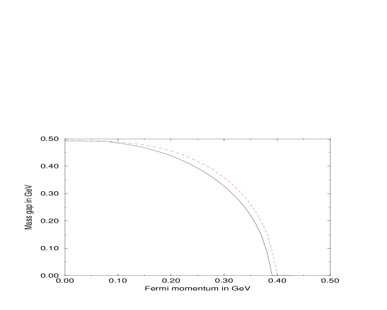
FIG. 5.: Mass gap $M$ as a function of fermi mometum. The dashed line correspond to no diqurak condensates. The solid line corresponds to both diquark and quark antiquark condensates structure for the ground state.

The solution of these equation at zero temperature is shown in Fig.(5) for the mass gap and in Fig.(6) for the superconducting gap. For the sake of comparision we have also plotted the mass gap without the diquark condensates. The coupling here taken as $g^{2}\sim 56GeV^{-2}$ and the cutoff$\Lambda\sim 0.67GeV$. these values are taken so as to give the same transition temperature as in ref[25, 31]. With these couplings, the mass gap at zero temperature and density is about 490 MeV and the mass gap vanishes at fermi momentum $k_{f}=\sqrt{\nu^{2}-M^{2}}=400MeV$. The corresponding critical quark number density is about $1.7/fm^{3}$.

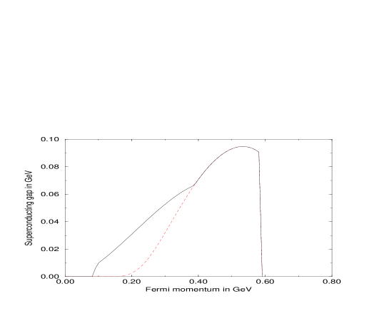
FIG. 6.: Superconducting gap $\Delta$ as a function of fermi mometum. The solid line corresponds to both diquark and quark antiquark condensates. The dashed line corresponds to only diquark condensates.

Presence of diquark condensate does not change these values very much. The diquark condensate increases with number density and becomes maximum of about 90 MeV beyond which the effect of the cutoff is felt and it vanishes for fermi momentum around 600 MeV. We also plot the equation of state (EOS) in Fig.7.

FIG. 7.: Pressure as a function of fermi momentum .

While plotting the EOS, we have added the bag constant $\epsilon_{0}$, which is the difference in energy density of the perturbative vacuum and the nonperturbative vacuum with condensate at zero temperature and density, to the pressure. With the present parameters the bag constant turns out to be $-(200MeV)^{4}$. The pressure has a cusp like structure and becomes negative at finite densities. The portion of the curve that goes down with $k_{f}$ corresponds to the nontrivial solution to the mass gap and the portion that increases with density correspond to zero mass solution. The negative pressure indicates mechanical instability and can have the interpretation that uniform nonzero density matter will break up in to droplets of finite density in which chiral symmetry is restored surrounded by empty space with zero pressure and density [25]. It is tempting to identify the droplets of quark matter with nucleons within which density is nozero and $\langle\bar{q}q\rangle=0$ – a fact reminscent of bag models [25]. Nothing in the model however says that the droplets have quark number three. The equation of state does not change much in presence of diquark condensates. This should be expected because the effect of diquark condensate is small in the region where chiral condensate is non vanishing. Thus gross structural properties of the neutron stars are not likely to be affected by diquark condensates. However, cooling of neutron stars shall be expected to be very much affected by such a gap of about 100 MeV.

V summary and discussions

We have looked into the structure of QCD vacuum in a nonperturbative manner with a variational ansatz. This has been done for zero temperature as well as finite temperature and densities. The input has been equal time algebra for the field operators and the ansatz for the ground state. At zero temperature, the Bogoliubov type pairing ansatz involving both quark and gluon condensates becomes energetically favourable beyond a critical coupling. It also gave some of the low energy hadronic properties like pion and proton charge raddi, proton,neutron magnetic moments and the bag constant to be around their phenomenological values for the coupling value of $1.28$. Thus $\alpha_{s}=1.28$ effectively corresponds to the QCD coupling constant for the vacuum configuration. With optimized renormalisation group equations, it has been seen that [33] $\alpha_{s}(Q)$ does not go to infinity as $Q$ decreases below 300 MeV, but freezes to a constant value around unity. Our analysis seems to remind us of a similar situation.

We next evaluated the correlation functions of hadronic currents in such a condensed medium. However it appears that to have quantitative agreement with correlator phenomenology, particularly in the pseudoscalar channel, these cannot be described by the propagators alone but must of necessity have the fluctuations of the condensates. This may be looked upon as combination of two effects –(i) an effective way of incorporating gluon condensate effects and (ii)the existance of explicit four point structure in QCD vacuum. In some ways these fluctuations may be related to the “hidden contributions” discussed by Suryak [10].

It is worthwhile pointing out that OPE and our approach are based on intrinsically different assumptions. The former is an expansion which separates short distance (Wilson coefficients) and long distance (condensates) physics. In our method we assume an explicit vacuum structure in terms of quark condensate (two point function) plus an irreducible four point function. Having made an ansatz for the vacuum, we do not make any further approximation in the evaluation of the correlators. The approach is phenomenological in the sense that the values of the parameters in the four point function [7] are chosen to reproduce the behaviour of the correlators. As emphasized by Shuryak [4] and Sch$\ddot{a}$fer and Shuryak [18] OPE is able to quantitatively describe the zero temperature pion correlation functions for small x (upto 0.25 fm) but underpredicts it for large x. In our work[6, 7] the agreement is quantitative with experimentally deduced mesonic correlation function and lattice results [3] for the whole range. This covers the small x values, resonance region and large x domain where the correlator vanishes. We have however more parameters. To the extent that the large x behaviour of the pionic correlator depends on gluon condensates in OPE our parametrization would imply an effective way of including gluon condensate effects.

For studying the correlators at finite temperature, we assume that the two point as well as the four point function vanish at $T=T_{C}$. The parameters in the four point function are assumed constant at their $T=0$ values – no additional T dependence is given to them. We see that our results are broadly in agreement with those of Hatsuda etal [17]. All the same, it is not possible to carry out a term by term comparison of our results with OPE results. This is because the assumptions are different in the two approaches. We recall that Hatsuda etal [17] attribute the decrease in the $\rho$ mass to contributions coming from four point function. They also find variation in the gluon condensates to be less than 5% over the temperature region that is considered. In our work we do not include the gluon condensates and the four point structure vanishes as $T\rightarrow T_{C}$. This is not the case for gluon condensate ($\langle GG\rangle$) in lattice calculations or in the dilute pion gas model of Ref. [17]. Consequently, we may be tempted to infer that the decrease in rho mass in our model is due to “genuine” four point function effects (as in Hatsuda etal [17]) and not from the “effective” gluon condensate contribution. One, however, has to be very cautious. This is because in the present work the parameters in the four point function were kept constant at their $T=0$ values. It should be recalled that these values were determined so as to correctly describe the behaviour of the correlators (in particular pion) at T=0. Hence the parameters do reflect some effective gluon condensate effects. The results at finite temperature would certainly be modified if these parameters are given significant T dependence. Our parametrization is such that if the parameters decrease with T then the contribution to the correlator will decrease. The crucial question however still remains as to the behaviour of $\langle GG\rangle$ for $T<T_{C}$. If it varies very little in this range then our assumption of the parameters remaining constant would be reasonable.

We would like to add here that the present analysis will be valid for temperatures below the critical temperature. Above the critical temperature there have been calculations essentially using finite temperature perturbative QCD in random phase approximations (RPA) [34]. However, in the region above $T_{C}$, nonperurbative features have been known to exist from studies in lattice QCD simulations[11]. In view of this, one may have to carry out a hard thermal loop calculation where a partial resummation is done[35]. Alternatively, one may use other nonperturbative approaches such as QCD sum rules at finite temperature [36] or RPA approach in an instanton liquid model for the QCD vacuum [19].

The vacuum structure at finite densities was looked into taking into account the possibility of diquark condensates in a Nambu-Jonalasinio model. As earlier, the approximation lies here only in the ansatz. The resulting gap equation for the superconducting gap is a relativistic generalisation of the BCS gap equation. The mass gap equation in the presence of superconducting gap is a new feature of the present calculation. Because of the point interaction as in ${\cal H}_{int}$ of Eq.(42)we could solve for the gap functions explicitly. In the presence of realistic potentials as in Ref.[37]or Ref.[38] one will have to solve an integral equation for the gap functions. Such a calculation is in progress [29]. It will be interesting to see how the results for the superconducting gap would be affected in presence of quark antiquark condensates as compared to the resummed perturbative QCD calculations at finite densities [27]. The equation of state here did not change very much. Thus the global properties of neutron stars shall not be affected in an appreciable manner. However, a gap of about 100 MeV can have its implications on neutron star cooloing [39], magnetic fields of pulsars and their thermal evolution [40]. Future theoretical studies of QCD at finite baryon densities may reveal to which extent these newly established features of quark matter considered in effective models shall have their correspondence in a more complete treatment of QCD at finite baryonic density and shed light on whether one may expect any distinguishing feature in the global properties of neutron/quark stars.

REFERENCES

- [1] R.P. Feynman, Nucl. Phys. B 188, 479 (1981)
- [2] M.A. Shifman, A.I. Vainshtein and V.I. Zakharov, Nucl. Phys. B147, 385, 448 and 519 (1979); R.A. Bertlmann, Acta Physica Austriaca 53, 305 (1981)
- [3] M.-C. Chu, J. M. Grandy, S. Huang and J. W. Negele, Phys. Rev. D48, 3340 (1993); ibid, Phys. Rev. D49, 6039 (1994)
- [4] E.V. Shuryak, Rev. Mod. Phys. 65, 1 (1993)
- [5] A. Mishra, H. Mishra, S.P. Misra, P.K. Panda and Varun Sheel, Int. J. of Mod. Phys. E 5, 93 (1996)
- [6] Varun Sheel, Hiranmaya Mishra and Jitendra C. Parikh, Int. J. Mod. Phys. E6, 275, (1997).
- [7] Varun Sheel, Hiranmaya Mishra and Jitendra C. Parikh, Phys. Lett. B382, 173 (1996).
- [8] V. Sheel, H. Mishra and J.C. Parikh, Phys. ReV D59,034501 (1999); ibidProg. Theor. Phys. Suppl.,129,137, (1997).
- [9] M. G. Mitchard, A. C. Davis and A. J. Macfarlane, Nucl. Phys. B 325, 470 (1989)
- [10] E.V. Shuryak and J.J.M. Verbaarschot, Nucl. Phys. B410, 37 (1993).
- [11] E. Laermann, Nucl. Phys. A610, 1c (1996).
- [12] E.V. Shuryak, Nucl. Phys. A544, 65c (1992).
- [13] T. Schfer and E.V. Shuryak, Phys. Rev. D54, 1099 (1996)
- [14] A.I. Bocharev nad M.E. Shaposhnikov, Nucl. Phys. B268, 220, 1986.
- [15] C. Adami, T. Hatsuda and I. Zahed, Phys. Rev. D43, 921 (1991) .
- [16] C. Adami, G.E. Brown, Phys. Rev. D46, 478 (1992) .
- [17] Tetsuo Hatsuda, Yuji Koike and Su Houng Lee, Nucl. Phys. B394, 221 (1993).
- [18] T. Schfer and E.V. Shuryak, Rev. Mod. Phys. 70, 223 (1998).
- [19] Velkovsky and E.V. Shuryak, Phys. Rev. D56, 2766 (1996).
- [20] H. Umezawa, H. Matsumoto and M. Tachiki Thermofield dynamics and condensed states (North Holland, Amsterdam, 1982) ; P.A. Henning, Phys. Rep.253, 235 (1995).
- [21] Amruta Mishra and Hiranmaya Mishra, J. Phys. G23,143, (1997).
- [22] P. Gerber and H. Leutwyler, Nucl. Phys. B321, 387 (1989).
- [23] T. Hatsuda and T. Kunihiro, Prog. Theor. Phys. Suppl. 91, 284 (1987).
- [24] D.Ballin and A. Love, Phys. rep. 107,325 (1984).
- [25] M. Alford, K.Rajagopal, F. Wilczek, Phys. Lett. B422,247(1998)i ibidNucl. Phys. B537,443 (1999).
- [26] R.Rapp, T.Schaefer, E. Suryak and M. Velkovsky Phys. Rev. Lett. 81, 53(1998),ibid,hep-ph/9904353.
- [27] D. Rische, R.D. Pisarski, Phys Rev D60,094013, 1999;ibid nucl-th/9910056, nucl-th/9907041.
- [28] D.I. Diakonov, H. Forkel, M.Lutz, Phys. Lett.B373,147 (1996).
- [29] H.Mishra and J.C. Parikh - in preparation
- [30] A.L. Fetter and J.D. Walecka, Quantum Theory of Many particle Systems(McGraw-Hill, New York, 1971.
- [31] T.M. Schwartz, S.P. Klevansky, G. Papp, Phys. Rev. C60,055205 (1999).
- [32] M. Asakawa and K. Yazaki, Nucl. Phys. A504,668 (1989).
- [33] A.C. Mattingly and P.M. Stevenson, Phys. Rev. Lett. 69, 1320 (1992); Phys. Rev. D 49, 437 (1994)
- [34] Jitendra C. Parikh, Philip J. Siemens, Phys. Rev. D37, 3246 (1988); R.B. Thayyullathil and J.C. Parikh, Phys. Rev. D44, 3964, (1991).
- [35] Eric Braaten and Robert D. Pisarski, Phys. rev. Lett. 64, 1338 (1990), Nucl. Phys. B339, 310 (1990).
- [36] J. Hansson and I. Zahed, “QCD sumrules at high temperature”, SUNY preprint, NTG 90-338 (1990).
- [37] R. Alkofer, P. A. Amundsen and K. Langfeld, Z. Phys. C 42, 199(1989), A.C. Davis and A.M. Matheson, Nucl. Phys. B246, 203 (1984).
- [38] A. Mishra, H. Mishra, S.P. Misra and S.N. Nayak, Z. Phys. C 57, 233 (1993); A. Mishra, H. Mishra and S.P. Misra, Z. Phys. C 58, 405 (1993)
- [39] D. Blashke, T. Klaehn and D.N. Voskorensky,astro-ph9908334.
- [40] D. Blashke, D.M. Sedrakian and K.M. Shahabasyan, astro-ph9904395, M.Alford, J. Berges and K.Rajagopal,astro-ph/9910254.