Correlation energy of the pairing Hamiltonian

Abstract

We study the correlation energy associated with the pair fluctuations in BCS theory. We use a schematic two-level pairing model and discuss the behavior of the correlation energy across shell closures, including the even-odd differences. It is shown that the random phase approximation (RPA) to the ground state energy reproduces the exact solutions quite well both in the normal fluid and in the superfluid phases. In marked contrast, other methods to improve the BCS energies, such as Lipkin-Nogami method, only work when the strength of a pairing interaction is large. We thus conclude that the RPA approach is better for a systematic theory of nuclear binding energies.

I Introduction

An important goal of nuclear theory is to predict nuclear binding energies. The mean-field approximation certainly provides a good starting point, but the correlation energy associated with nearly degenerate configurations can be of the order of several MeV. Since one would like an order of magnitude better accuracy for global modeling, the correlations must be treated with some care. The correlations associated with broken mean-field symmetries, namely center-of-mass localization, deformations, and pairing, are especially important and need to be singled out for special attention. The study of such correlation effects has attracted much interest, see Refs. [1, 2, 3] for recent citations. Popular computational methods include the generator coordinate method (GCM)[7], variation-with-projection methods (e.g., VAP) [8], and the RPA [9].

In previous work[10], we have advocated the RPA approach for deformations and for center-of-mass localization. The correlation energy is calculated from the RPA formula [9]

$$E_{corr}=\frac{1}{2}\left(\sum_{i}\hbar\omega_{i}-Tr(A)\right),$$ (1)

where $\omega_{i}$ is the frequency of the RPA phonon and $A$ is the $A$ matrix in the RPA equations. This method requires solving the RPA equations for each nucleus, which is computationally easy if the interaction is assumed to be separable[11, 12, 13]. On other other hand, methods such as VAP and GCM are rather complicated to apply. One should also remember that a global theory requires a method that is not only systematic but also preserves the relative computational simplicity of the mean field approximation. In this respect, the Lipkin-Nogami method is a popular candidate for a computationally easy method to go beyond the mean field pairing theory[14, 15, 16] .

In this paper, we continue our study of the accuracy of the RPA correlation formula (1), going on to pairing correlations. There is a long history of the RPA treatment of pairing correlations. An early study by Bang and Krumlinde [17] showed that the RPA formula reproduces the exact correlation energy rather well in a schematic model. Kyotoku et al. [18] compared the leading $1/N$ behavior of different methods including the Lipkin-Nogami method. They found that only RPA gave the exact coefficient in the condensed phase. The RPA method has in fact been used in realistic models of deformed nuclei[19]. The RPA correlation in the normal phase was studied in Ref. [20] using the self-consistent version of RPA. But perhaps surprisingly in view of the large literature, we have not found any studies that specifically compare the RPA with the computationally attractive alternative methods, testing the behavior across shell closures and for odd $N$ systems. It is important that the method should not introduce spurious discontinuities when the mean field solution changes character; otherwise separation energies could not be reliably calculated [21].

To investigate the applicability of Eq. (1) and study the effects of symmetry breaking restoration, in this paper we employ a well-known schematic two-level pairing model[16, 20, 22, 23, 24, 25, 26, 27], and compare its exact solutions to the approximations that are computationally attractive. The details of the RPA correlation energy are given in the next section. They include both the quasi-particle RPA extension of the BCS theory and the RPA for the pairing Hamiltonian when the strength is too weak for the mean field approximation to support the BCS solution (the “pairing-vibration” regime). The specific application of the various methods to the two-level model is given in the following section III.

II Pairing Hamiltonian and the RPA

The pairing Hamiltonian and the BCS solution are well-known and we just summarize the equations to confirm the standard notation. In this paper we consider a Hamiltonian with an arbitrary single-particle term but a pairing interaction whose strength is state-independent,

$$H=\sum_{j}\epsilon_{j}\hat{N}_{j}-G\sum_{j,j^{\prime}}A_{j}^{\dagger}A_{j^{\prime}},$$ (2)

where $\epsilon_{j}$ is a single-particle energy. The number operator $\hat{N}_{j}$ for the shell $j$ is given by

$$\hat{N}_{j}=\sum_{m>0}\left(a_{jm}^{\dagger}a_{jm}+a^{\dagger}_{j\bar{m}}a_{j\bar{m}}\right).$$ (3)

Here, $a_{j\bar{m}}$ is the annihilation operator for the time-reversal state and is given by $a_{j\bar{m}}=(-)^{j-m}a_{j-m}$. The pairing operator $A_{j}^{\dagger}$ in the Hamiltonian (2) is given by

$$A_{j}^{\dagger}=\sum_{m>0}a^{\dagger}_{jm}a^{\dagger}_{j\bar{m}},$$ (4)

and $A_{j}$ is the Hermitian conjugate of $A_{j}^{\dagger}$. The exact solutions of the Hamiltonian were obtained a long time ago by Richardson and Sherman[4]. In Appendix A, we solve the Richardson equation for a simple, but non-trivial case where there are two pairs in a single $j$-shell.

The BCS theory is the mean field solution to Eq. (2). We remind the reader that it is derived variationally from a ground state wave function of the form

$$|BCS\rangle=\prod_{j,m>0}(u_{j}+v_{j}a^{\dagger}_{jm}a^{\dagger}_{j\bar{m}})|\rangle,$$ (5)

where $v_{j}$ is the usual pair occupation amplitude and $u_{j}$ satisfies $u_{j}^{2}+v_{j}^{2}=1$. This wave function is appropriate for even-$N$ systems, $N$ being the number of particles in a system. The extension to odd-$N$ systems is given at the end of this subsection. Important quantities in the variational solution are the chemical potential $\lambda$ and the pairing gap $\Delta=G\sum_{j}\Omega_{j}u_{j}v_{j}$, $\Omega_{j}=(2j+1)/2$ being the pair degeneracy of the $j$-shell. When the pairing strength $G$ is small, the variational equations only have the trivial solution, $v_{j},u_{j}=0$ or 1 and $\Delta=0$. The ground state wave function is thus given by $|HF\rangle=\prod_{j,m}a_{jm}^{\dagger}|\rangle$ and the ground state energy is obtained as

$$E_{HF}=\langle HF|H|HF\rangle=\sum_{j:occupied}\Omega_{j}(2\epsilon_{j}-G).$$ (6)

When the strength of the pairing interaction $G$ is larger than some critical value $G_{crit}$, the variational equations have a non-trivial solution $\Delta\neq 0$ and the ground state energy is given by

$$E_{BCS}=\langle BCS|H|BCS\rangle=2\sum_{j}\Omega_{j}\epsilon_{j}v_{j}^{2}-\frac{\Delta^{2}}{G}-G\sum_{j}\Omega_{j}v_{j}^{4}.$$ (7)

For odd $N$ systems, one of the particles in a system does not form a pair and blocks a level. When the $k$-th level is blocked, the HF energy, the BCS energy, and the pairing gap are modified to

$$E_{HF} = \sum_{j:occupied}\widetilde{\Omega}_{j}(2\epsilon_{j}-G)+\epsilon_{k},$$ (8)

$$E_{BCS} = 2\sum_{j}\widetilde{\Omega}_{j}\epsilon_{j}v_{j}^{2}-\frac{\Delta^{2}}{G}-G\sum_{j}\widetilde{\Omega}_{j}v_{j}^{4}+\epsilon_{k},$$ (9)

$$\Delta = G\sum_{j}\widetilde{\Omega}_{j}u_{j}v_{j},$$ (10)

respectively. Here, $\widetilde{\Omega}_{j}=\Omega_{j}$ for $j\neq k$, and $\widetilde{\Omega}_{k}=\Omega_{k}-\delta_{N,odd}$. The chemical potential $\lambda$ is determined so that

$$\sum_{j}\widetilde{\Omega}_{j}v_{j}^{2}+1=N,$$ (11)

is satisfied. This formalism is referred to as the blocked-BCS theory.

A Random phase approximation

We next introduce the random phase approximation to compute the correlation energy. Let us first consider the RPA in the superfluid phase (QRPA). We refer to Refs. [7, 22, 28] for the formulation. The result is the well-known RPA matrix equation

$$\left(\begin{array}[]{cc}A&B\\ -B&-A\end{array}\right)\left(\begin{array}[]{c}X\\ Y\end{array}\right)=\hbar\omega\left(\begin{array}[]{c}X\\ Y\end{array}\right),$$ (12)

where the matrices $A$ and $B$ are given by

$$A_{ij} = 2E_{i}\delta_{i,j}-G\sqrt{\widetilde{\Omega}_{i}}\sqrt{\widetilde{\Omega}_{j}}(u_{i}^{2}u_{j}^{2}+v_{i}^{2}v_{j}^{2}),$$ (13)

$$B_{ij} = G\sqrt{\widetilde{\Omega}_{i}}\sqrt{\widetilde{\Omega}_{j}}(u_{i}^{2}v_{j}^{2}+v_{i}^{2}u_{j}^{2}),$$ (14)

respectively. Here, $\widetilde{\Omega}_{j}$ is defined in the previous subsection, and $E_{j}=\sqrt{(\epsilon_{j}-\lambda-Gv_{j}^{2})^{2}+\Delta^{2}}$ is the quasi-particle energy. The RPA excitation operator $Q^{\dagger}$ is given in terms of quasi-particle operators

$$\alpha_{jm}^{\dagger} = u_{j}a^{\dagger}_{jm}-v_{j}a_{j\bar{m}},$$ (15)

$$\alpha_{j\bar{m}}^{\dagger} = u_{j}a^{\dagger}_{j\bar{m}}+v_{j}a_{jm},$$ (16)

as

$$Q^{\dagger}=\sum_{j}\left(X_{j}\sum_{m}\alpha_{jm}^{\dagger}\alpha_{j\bar{m}}^{\dagger}-Y_{j}\sum_{m}\alpha_{j\bar{m}}\alpha_{jm}\right)/\sqrt{\widetilde{\Omega}_{j}}.$$ (17)

The QRPA correlation energy is given by Eq. (1) with the $A$ matrix given by Eq. (13). Note that the second term on the right hand side of Eq. (1) is not $\sum_{i}2E_{i}$ but $Tr(A)$. This point was overlooked in the integral approaches to the correlation energy in Refs. [11, 12].

We next consider the RPA in a normal-fluid phase (pp-RPA), which describes pairing vibrations. The equation for the pp-RPA can be obtained from the QRPA equation by setting $\Delta=0$ and $v_{h}=u_{p}=1$, where $p$ and $h$ denote particle and hole states, respectively. As for the chemical potential $\lambda$, there is no definite value for it in the normal fluid phase since it can be anywhere between the highest occupied and the lowest unoccupied levels. Notice, however, that the pairing vibration describes the ground state in the $N\pm 2$ systems and the role of the chemical potential is therefore just to shift the energies by an amount $\pm 2\lambda$. After removing these trivial energy shifts, one obtains

$$A_{pp^{\prime}} = 2\epsilon_{p}\delta_{p,p^{\prime}}-G\sqrt{\widetilde{\Omega}_{p}}\sqrt{\widetilde{\Omega}_{p^{\prime}}},$$ (18)

$$A_{hh^{\prime}} = -2(\epsilon_{h}-G)\delta_{h,h^{\prime}}-G\sqrt{\widetilde{\Omega}_{h}}\sqrt{\widetilde{\Omega}_{h^{\prime}}},$$ (19)

$$B_{ph} = G\sqrt{\widetilde{\Omega}_{p}}\sqrt{\widetilde{\Omega}_{h}},$$ (20)

$$A_{ph} = B_{pp^{\prime}}=B_{hh^{\prime}}=0.$$ (21)

This $2(N_{p}+N_{h})\times 2(N_{p}+N_{h})$ dimensional matrix equation, where $N_{p}$ is the number of unoccupied shells and $N_{h}$ is that of occupied shells, can be decoupled into two $(N_{p}+N_{h})\times(N_{p}+N_{h})$ matrix equations as

$$\left(\begin{array}[]{cc}A&-B\\ B&-C\end{array}\right)\left(\begin{array}[]{c}X^{a}\\ Y^{a}\end{array}\right)=\hbar\omega_{a}\left(\begin{array}[]{c}X^{a}\\ Y^{a}\end{array}\right),$$ (22)

and

$$\left(\begin{array}[]{cc}C&-B\\ B&-A\end{array}\right)\left(\begin{array}[]{c}X^{r}\\ Y^{r}\end{array}\right)=\hbar\omega_{r}\left(\begin{array}[]{c}X^{r}\\ Y^{r}\end{array}\right).$$ (23)

Here, the matrix $C$ is defined as $C_{hh^{\prime}}=A_{hh^{\prime}},C_{ph}=0$, and RPA amplitudes are given by $X^{a}_{p}=X_{p},Y^{a}_{h}=-Y_{h},X^{r}_{h}=-X_{h}$, and $Y^{r}_{p}=Y_{p}$. The first equation (22) describes the ground state of the $N+2$ system and is referred to as the addition mode, while the second equation (23) describes the $N-2$ system and is called the removal mode. Noticing that Eq. (1) is a half of a sum of the difference between the RPA and the Tamm-Dancoff approximation (TDA) frequencies for each mode of excitation [7], we find the correlation energy for the addition mode to be

$$E^{a}_{corr}=\frac{1}{2}\left(\sum_{i}\hbar\omega_{ai}-Tr(A)\right),$$ (24)

while that for the removal mode is

$$E^{r}_{corr}=\frac{1}{2}\left(\sum_{i}\hbar\omega_{ri}-Tr(C)\right).$$ (25)

The total correlation energy is the sum of these, $E_{corr}=E^{a}_{corr}+E^{r}_{corr}$.

Typically, one finds that an RPA mode goes to zero frequency at the mean-field phase transition. This is not the case for Eqs. (22) and (23), thus giving a discontinuity in the frequencies at the transition. However, as we have mentioned above, this is an artifact of an awkward choice of the chemical potential $\lambda$, and it will be the case that the sum of an addition and removal mode goes to zero.

B Lipkin-Nogami method

An alternative way to restore the broken gauge symmetry of the BCS approximation is to carry out the number projection of the BCS wave function. The Lipkin-Nogami method provides an approximate way for number projection. It was first invented by Lipkin [14], and was developed by Nogami and his collaborators [15, 16]. Because of its relative simplicity, it has been widely applied [24, 31, 32, 33, 34].

In the Lipkin-Nogami method, the expectation value $\langle H-\lambda\hat{N}-\lambda_{2}\hat{N}^{2}\rangle_{BCS}$ is varied. The resultant equations to be solved are given by [16]

$$\frac{2}{G}=\sum_{j}\frac{\widetilde{\Omega}_{j}}{\sqrt{\tilde{\epsilon}_{j}+\Delta^{2}}},$$ (26)

$$2\sum_{j}\widetilde{\Omega}_{j}v_{j}^{2}+\delta_{N,odd}=N,$$ (27)

$$\lambda_{2}=\frac{G}{4}\left\{\frac{\left(\sum_{i}\widetilde{\Omega}_{i}u_{i}^{3}v_{i}\right)\left(\sum_{i}\widetilde{\Omega}_{i}u_{i}v_{i}^{3}\right)-\sum_{i}\widetilde{\Omega}_{i}u_{i}^{4}v_{i}^{4}}{\left(\sum_{i}\widetilde{\Omega}_{i}u_{i}^{2}v_{i}^{2}\right)^{2}-\sum_{i}\widetilde{\Omega}_{i}u_{i}^{4}v_{i}^{4}}\right\},$$ (28)

where $\tilde{\epsilon}_{i},v_{i}$, and $u_{i}$ are defined as

$$\tilde{\epsilon}_{i} = \epsilon_{i}+(4\lambda_{2}-G)v_{i}^{2}-\lambda,$$ (29)

$$v_{i}^{2} = \frac{1}{2}\left(1-\frac{\tilde{\epsilon}_{i}}{\sqrt{\tilde{\epsilon}_{i}^{2}+\Delta^{2}}}\right),$$ (30)

$$u_{i}^{2} = 1-v_{i}^{2},$$ (31)

respectively. We use the blocked-Lipkin-Nogami prescription for odd $N$ systems. One of the characteristic features of the Lipkin-Nogami method is that the pairing gap $\Delta$ has a finite value even in the weak $G$ limit where $\Delta$ is zero in the BCS approximation. The ground state energy in the Lipkin-Nogami method is given by

$$E_{LN}=2\sum_{j}\widetilde{\Omega}_{j}\epsilon_{j}v_{j}^{2}-\frac{\Delta^{2}}{G}-G\sum_{j}\widetilde{\Omega}_{j}v_{j}^{4}-4\lambda_{2}\sum_{j}\widetilde{\Omega}_{j}u_{j}^{2}v_{j}^{2}+\epsilon_{k}\delta_{N,odd}.$$ (32)

III Two-level pairing model

We now apply the above equations to a schematic two-level model. This model was first introduced in Ref.[22], and has been used in the literature to test several approximations [16, 18, 20, 23, 24, 25, 26, 27]. We label the lower and the higher levels 1 and 2, taking $\epsilon_{1}=-\epsilon/2,\epsilon_{2}=\epsilon/2$. The Hamiltonian can be numerically diagonalised using the quasi-spin formalism [7]. The basis states are denoted by $|S_{1}S_{10};S_{2}S_{20}\rangle$, where $S_{i}$ and $S_{i0}$ are defined by $S_{i}=(\Omega_{i}-\nu_{i})/2$ and $S_{i0}=(N_{i}-\Omega_{i})/2$, respectively. The latter takes a value of $-S_{i},-S_{i}+1,\cdots,S_{i}$. $\nu_{i}$ is the seniority quantum number. For the ground state of even-$N$ systems, the total seniority $\nu_{1}+\nu_{2}$ is 0, while it is 1 for odd-$N$ systems. The matrix elements of the Hamiltonian read

$$\langle S_{1}^{\prime}S_{10}^{\prime};S_{2}^{\prime}S_{20}^{\prime}|H|S_{1}S_{10};S_{2}S_{20}\rangle=\delta_{S_{1},S_{1}^{\prime}}\delta_{S_{2},S_{2}^{\prime}}\left\{\epsilon\left(S_{20}-S_{10}-\frac{\Omega_{1}-\Omega_{2}}{2}\right)\delta_{S_{10},S_{10}^{\prime}}\delta_{S_{20},S_{20}^{\prime}}\right.$$ (33)

$$\quad\quad-G\left(S_{1}(S_{1}+1)-S_{10}(S_{10}+1)+S_{2}(S_{2}+1)-S_{20}(S_{20}+1)\right)\delta_{S_{10},S_{10}^{\prime}}\delta_{S_{20},S_{20}^{\prime}}$$ (34)

$$\quad\quad-G\sqrt{(S_{1}(S_{1}+1)-S_{10}(S_{10}-1)}\sqrt{S_{2}(S_{2}+1)-S_{20}(S_{20}+1)}\delta_{S_{10},S_{10}^{\prime}+1}\delta_{S_{20},S_{20}^{\prime}-1}$$ (35)

$$\quad\quad\left.-G\sqrt{(S_{1}(S_{1}+1)-S_{10}(S_{10}+1)}\sqrt{S_{2}(S_{2}+1)-S_{20}(S_{20}-1)}\delta_{S_{10},S_{10}^{\prime}-1}\delta_{S_{20},S_{20}^{\prime}+1}\right\}.$$ (36)

We first consider a symmetric two-level problem i.e., $\Omega_{1}=\Omega_{2}=\Omega$, and assume the number of fermionic particle is $N=2\Omega$. Equations for several approximations can be solved analytically for such a system. The gap equation in the BCS theory leads to a pairing gap of

$$\Delta=\sqrt{G^{2}\Omega^{2}-\frac{\tilde{\epsilon}^{2}}{4}},$$ (37)

together with

$$v_{1}^{2} = u_{2}^{2}=\frac{1}{2}\left(1+\frac{\tilde{\epsilon}}{2G\Omega}\right)\equiv v^{2},$$ (38)

$$u_{1}^{2} = v_{2}^{2}=\frac{1}{2}\left(1-\frac{\tilde{\epsilon}}{2G\Omega}\right)\equiv u^{2}.$$ (39)

$$\lambda = \frac{\tilde{\epsilon}-\epsilon}{2}-Gv^{2},$$ (40)

where $\tilde{\epsilon}$ is defined as $\tilde{\epsilon}=2\Omega\epsilon/(2\Omega-1)$.

From Eq. (37), one can find the critical strength of the phase transition to be $G_{crit}=\epsilon/(2\Omega-1)$. For $G$ larger than $G_{crit}$, the system is in the superfluid phase, and the matrices $A$ and $B$ for the QRPA equation are given by (see Eqs. (13) and (14))

$$A_{11} = A_{22}=G\Omega-\frac{\Delta^{2}}{2G\Omega^{2}}+\frac{\Delta^{2}}{2G\Omega},$$ (41)

$$A_{12} = A_{21}=-\frac{\Delta^{2}}{2G\Omega},$$ (42)

$$B_{11} = B_{22}=-\frac{\Delta^{2}}{2G\Omega^{2}}+\frac{\Delta^{2}}{2G\Omega},$$ (43)

$$B_{12} = B_{21}=G\Omega-\frac{\Delta^{2}}{2G\Omega},$$ (44)

The solutions of the QRPA equation are $\hbar\omega=0$ and $\sqrt{4\Delta^{2}-2\Delta^{2}/\Omega}$, from which the correlation energy is computed as

$$E_{corr}=\sqrt{\Delta^{2}-\Delta^{2}/2\Omega}-G\Omega+\frac{\Delta^{2}}{2G\Omega^{2}}-\frac{\Delta^{2}}{2G\Omega}.$$ (45)

When the strength of the pairing interaction $G$ is smaller than $G_{crit}$, the system is in the normal fluid phase. The mean field energy is then evaluated as $E_{HF}=-\epsilon\Omega-G\Omega$. For the present two-level model, the $A,B$, and $C$ matrices for the pp-RPA are just numbers and are given by $A=\epsilon-G\Omega$, $B=G\Omega$, and $C=\epsilon-G\Omega+2G$, respectively. The frequencies for the addition and the removal modes are then found to be

$$\hbar\omega_{a} = -G+\sqrt{\epsilon+G}\sqrt{\epsilon+G-2G\Omega},$$ (46)

$$\hbar\omega_{r} = G+\sqrt{\epsilon+G}\sqrt{\epsilon+G-2G\Omega},$$ (47)

respectively. The total correlation energy is thus obtained as

$$E_{corr}=\sqrt{\epsilon+G}\sqrt{\epsilon+G-2G\Omega}-(\epsilon-G\Omega+G).$$ (48)

Figure 1 shows the RPA frequencies for each modes of excitation as a function of $G$, for $\Omega$ = 8. As we noted in the previous section, we see that because of the chemical potential the pp-RPA frequencies do not match with the QRPA frequencies at the critical point of phase transition from a normal-fluid to a superfluid phases. Figure 2 compares the ground state energy obtained by several methods. The solid line is the exact solution obtained by numerically diagonalizing the Hamiltonian. The dashed line is the ground state energy in the mean field BCS approximation. It considerably deviates from the exact solution through the entire range of $G$ shown in the figure. The dot-dashed line takes into account the RPA correlation energy in addition to the mean field energy. It reproduces very well the exact solutions, except in the vicinity of the critical point of the phase transition. Around the critical point, one would need to compute the correlation energy with some care, using e.g., the self-consistent RPA discussed in Ref. [20] which removes the cusp behaviour of the RPA frequency around the critical strength.

It is interesting to compare the present mean field plus RPA approach with the Lipkin-Nogami method. The equations for the Lipkin-Nogami method for the two-level model were solved in Ref. [16]. The results are given by

$$\Delta^{2} = (G\Omega)^{2}(1-\tilde{\kappa}^{2}),$$ (49)

$$v_{1}^{2} = u_{2}^{2}=(1+\tilde{\kappa})/2,$$ (50)

$$u_{1}^{2} = v_{2}^{2}=(1-\tilde{\kappa})/2,$$ (51)

$$4\lambda_{2}-G = \frac{2G\Omega\tilde{\kappa}^{2}}{(2\Omega-1)(1-\tilde{\kappa}^{2})},$$ (52)

where $\tilde{\kappa}$ is the physical solution, which satisfies $0\leq\tilde{\kappa}\leq 1$, of an equation

$$2(1-\Omega)\tilde{\kappa}^{3}+(2\Omega-1)\kappa\tilde{\kappa}^{2}+(2\Omega-1)\tilde{\kappa}-(2\Omega-1)\kappa=0,$$ (53)

and $\kappa$ is defined as $\epsilon/2G\Omega$. The ground state energy in the Lipkin-Nogami method given by Eq. (32) is denoted by the thin solid line in Fig. 2. Although it reproduces the exact results for large values of $G$, it deviates significantly from them for small values. This behaviour is consistent with the numerical observation in Ref. [24] as well as the result of Ref.[18] where it was found that the Lipkin-Nogami method is only correct in the limit of a strong pairing force. In marked contrast, the ground state energy in the BCS plus QRPA coincides with the exact solution at the leading order of an expansion in 1/$\Omega$ for any strength of the pairing interaction as long as it is larger than the critical value [18].

From Fig. 2, it is unclear whether the Lipkin-Nogami method or RPA are more accurate for purposes of a global theory of binding. So we now consider a more realistic situation, varying the particle number $N$ rather than the interaction strength $G$. We consider the paring energy in oxygen isotopes, taking the neutron 1p and 2s-1d shells as the lower and higher levels of the two-level model. The pair degeneracy $\Omega$ thus reads $\Omega_{1}=3$ and $\Omega_{2}=6$, and the number of particle in a system is given by $N=A-8-2$ for the ^AO nucleus. We assume that the energy difference between the two levels $\epsilon$ is given by $\epsilon=41A^{-1/3}$ and the pairing strength $G=23/A$. The upper panel of Fig. 3 shows the ground state energy as a function of $A$. In order to match with the experimental data for the ¹⁶O nucleus, we have added a constant $-72.8$ MeV to the Hamiltonian for all the isotopes. The exact solutions are denoted by the filled circles. The deviation from the BCS approximation (the dashed line) is around 2 MeV for even $A$ systems and it is around 1.2 MeV for odd $A$ systems. This value varies within about 0.5 MeV along the isotopes and shows relatively strong $A$ dependence. One can notice that the RPA approach (the dot-dashed line) reproduces quite well the exact solutions. On the contrary, the Lipkin-Nogami approach (the thin solid line) is much less satisfactory and shows a different $A$ dependence from the exact results. The pairing gaps $\Delta$ in the BCS approximation and in the Lipkin-Nogami method are shown separately in the lower panel of Fig. 3. For the Lipkin-Nogami method, we show $\Delta+\lambda_{2}$, which is to be compared with experimental data [15, 16]. The closed shell nucleus ¹⁶O and its neighbour nuclei ^15,17O have a zero pairing gap in the BCS approximation, and the Lipkin-Nogami method does not work well for these nuclei, as can be casted in Fig. 2. On the other hand, the RPA approach reproduces the correct $A$ dependence of the binding energy. Evidently, the RPA formula provides a better method to compute correlation energies than the Lipkin-Nogami method, especially for shell closures.

IV Summary

Returning to our initial motivation, we seek a computationally tractable way to include pairing effects in a global model of nuclear binding energies, going beyond the BCS theory. Two attractive possibilities are the Lipkin-Nogami method and the RPA, in particular if the pairing interaction has a separable form. In this paper, we used a solvable two-level pairing Hamiltonian to show that the RPA formula for the correlation energy reproduces well the exact solutions both in a normal-fluid and a superfluid phases. On the contrary, the Lipkin-Nogami method is considerably less accurate for weak pairing, and therefore is not suitable in transition regions. As a consequence, the Lipkin-Nogami method fails to reproduce the correct mass number dependence of the binding energy around a shell closure. The correlation energy associated with the number fluctuation for the neutron mode in O isotopes was shown to be order of 2 MeV and has a relatively strong mass dependence. Although the correlation energy is small compared with the absolute value of the ground state energy, this suggests that including the correlation energy in the RPA provides a promising way to develop a better microscopic systematic theory for nuclear binding energies.

A Richardson solution

For a system where the number of pairs is $N_{pair}$, i.e., a 2$N_{pair}$-fermion system, the ground state energy of the Hamiltonian (2) is given by [5, 6]

$$E_{gs}=\sum_{\lambda=1}^{N_{pair}}z_{\lambda},$$ (A1)

where $z_{\lambda}$ are $N_{pair}$ solutions of $N_{pair}$ coupled equations given by

$$\sum_{j}\frac{\Omega_{j}}{2\epsilon_{j}-z_{\lambda}}-\mathop{{\;\,{\sum}^{\prime}}}_{\lambda^{\prime}}\frac{2}{z_{\lambda^{\prime}}-z_{\lambda}}=\frac{1}{G}.$$ (A2)

The prime in the summation of $\lambda^{\prime}$ means to take only those $\lambda^{\prime}$ which are different from $\lambda$, and $\Omega_{j}=(2j+1)/2$ is the pair degeneracy of the $j$-shell. In general, $z_{\lambda}$ are complex.

For a two pair system ($N_{pair}$=2) in a single $j$-shell, setting $\epsilon_{j}=0$ and $\Omega_{j}=\Omega$, the Richardson equation reads

$$-\frac{\Omega}{z_{1}}-\frac{2}{z_{2}-z_{1}} = \frac{1}{G}$$ (A3)

$$-\frac{\Omega}{z_{2}}-\frac{2}{z_{1}-z_{2}} = \frac{1}{G}.$$ (A4)

The solutions of these equations are found to be

$$z=-G(\Omega-1)\pm i\sqrt{G^{2}(\Omega-1)},$$ (A5)

from which the ground state energy reads $E_{gs}=-2G(\Omega-1)$. This result coincides with the solution obtained using the seniority scheme,

$$E(N_{pair})=-G\left\{\frac{\Omega}{2}\left(\frac{\Omega}{2}+1\right)-\frac{1}{4}(2N_{pair}-\Omega)^{2}+\frac{1}{2}(2N_{pair}-\Omega)\right\}.$$ (A6)

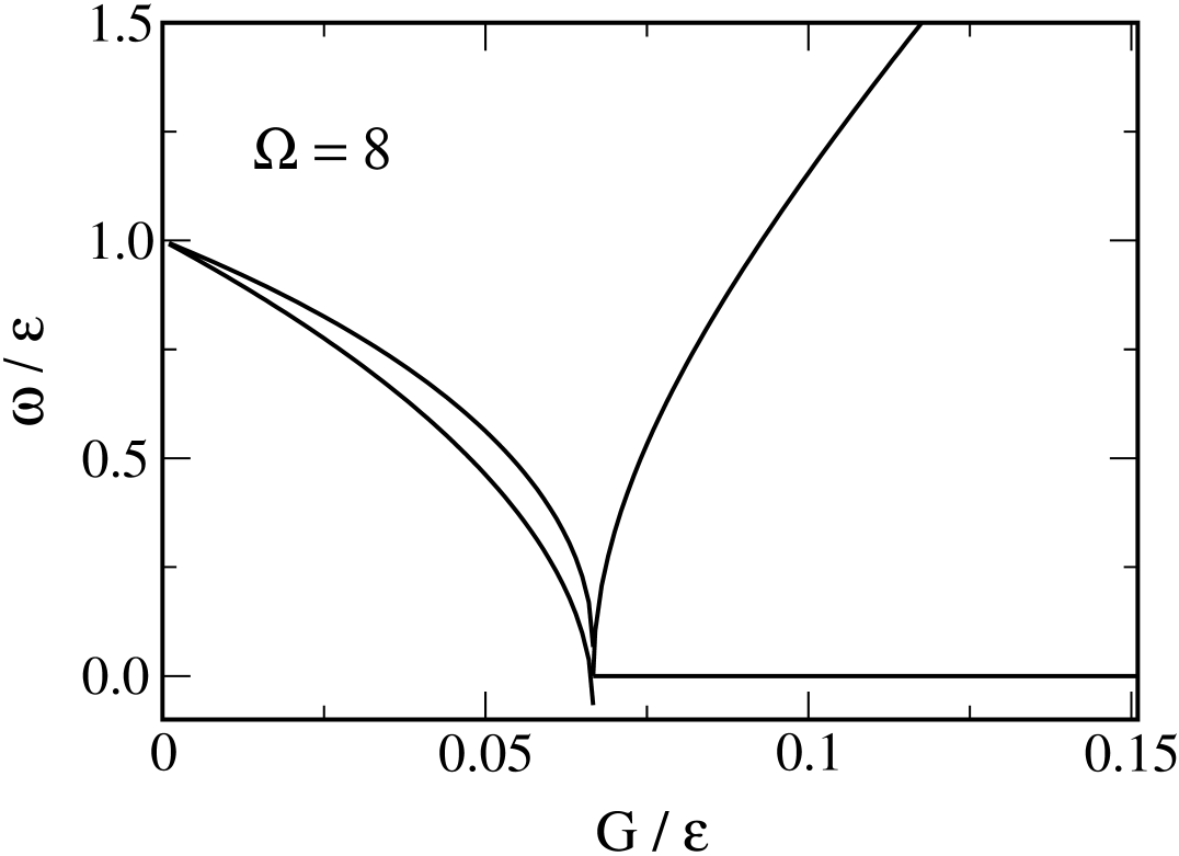
FIG. 1.: RPA frequencies as a function of the strength of the pairing interaction $G$ for a two-level system. The pair degeneracy $\Omega$ is set to be 8. The strength of the pairing interaction $G$ is given in the unit of $\epsilon$.

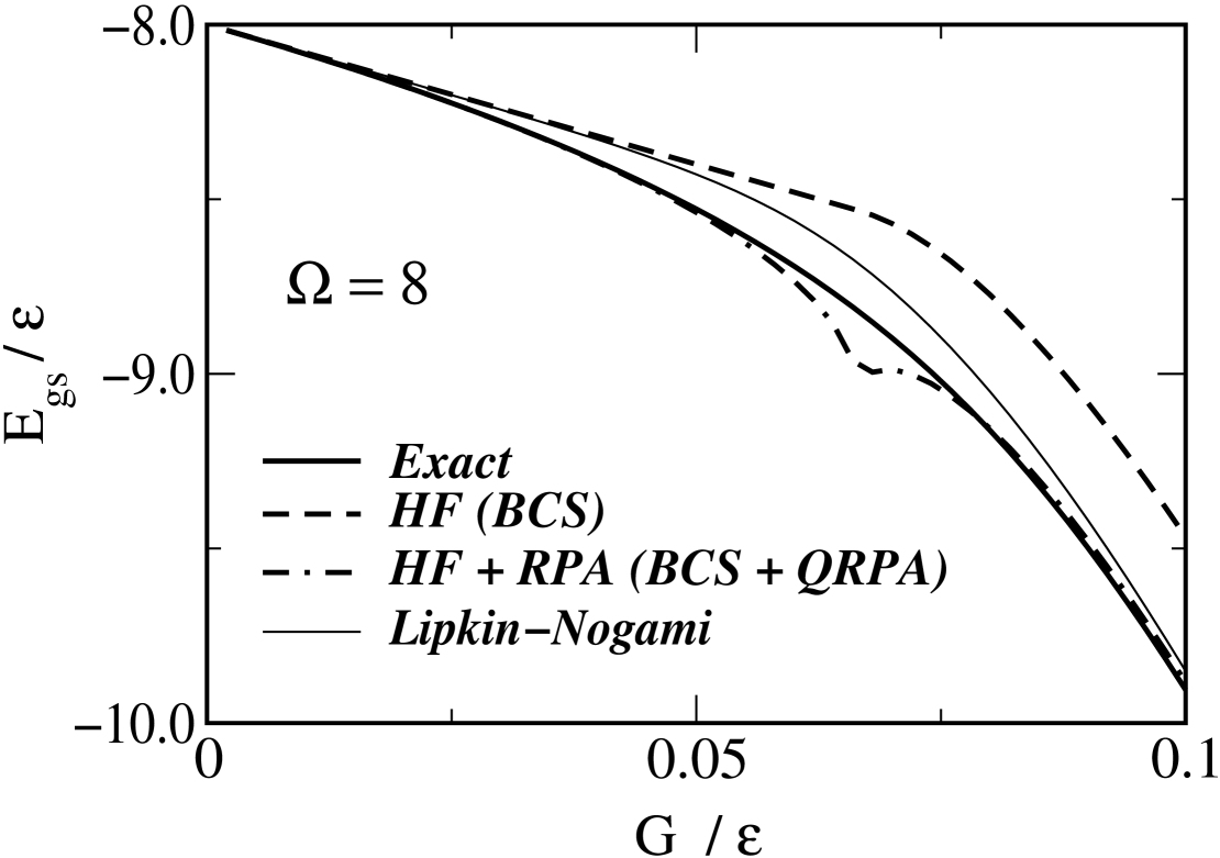
FIG. 2.: Comparison of the ground state energy $E_{gs}$ obtained by several methods. The solid line is the exact numerical solution, while the ground state energy in the Hartree-Fock (BCS) approximation is denoted by the dashed line. The dot-dashed line takes the RPA correlation energy into account in addition to the HF (BCS) energy. The results of the Lipkin-Nogami method are denoted by the thin solid line.

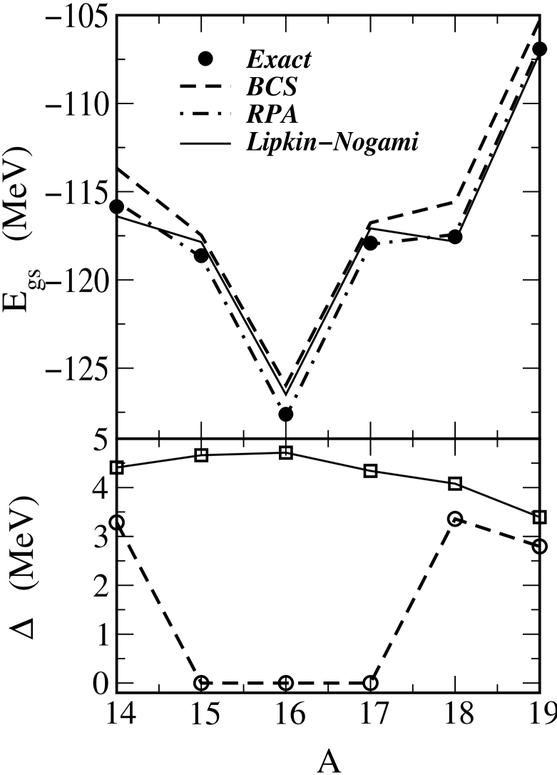
FIG. 3.: The ground state energy $E_{gs}$ (the upper panel) and the pairing gap (the lower panel) for oxygen isotopes estimated with the two-level model as a function of the mass number. The exact reults are denoted by the filled circles, while the meaning of each line is the same as in Fig. 2. For the pairing gap in the Lipkin-Nogami method, $\lambda_{2}$ is added to the pairing gap $\Delta$.

REFERENCES

- [1] M. Bender, K. Rutz, P.-G. Reinhard, and J.A. Maruhn, Euro. Phys. A7 (2000) 467.
- [2] A. Valor, P.-H. Heenen, and P. Bonche, Nucl. Phys. A671 (2000) 145; P.-H. Heenen, P. Bonche, S. Cwiok, W. Nazarewicz, and A. Valor, RIKEN Review 26 (2000) 31.
- [3] R. Rodringuez-Guzman, J.L. Egido, and L.M. Robledo, Phys. Lett. B474 (2000) 15.
- [4] R.W. Richardson and N. Sherman, Nucl. Phys. 52 (1964) 221.
- [5] R.W. Richardson, J. Math. Phys. 18 (1977) 1802.
- [6] F. Pan and J.P. Draayer, Phys. Lett. B442 (1998) 7.
- [7] P. Ring and P. Schuck, The Nuclear Many Body Problem (Springer-Verlag, New York, 1980).
- [8] R. Balian, H. Flocard, and M. Vénéroni, Phys. Rep. 317 (1999) 251.
- [9] D.J. Rowe, Phys. Rev. 175 (1968) 1283.
- [10] K. Hagino and G.F. Bertsch, Phys. Rev. C61 (2000) 024307.
- [11] F. Dönau, D. Almehed, and R.G. Nazmitdinov, Phys. Rev. Lett. 83 (1999) 280.
- [12] Y.R. Shimizu, P. Donati, and R.A. Broglia, nucl-th/9911039.
- [13] C.W. Johnson, G.F. Bertsch, and W.D. Hazelton, Comp. Phys. Comm. 120 (1999) 155.
- [14] H.J. Lipkin, Ann. Phys. (N.Y.) 9 (1960) 272.
- [15] Y. Nogami, Phys. Rev. 134 (1964) B313.
- [16] H.C. Pradhan, Y. Nogami, and J. Law, Nucl. Phys. A201 (1973) 357.
- [17] J. Bang and J. Krumlinde, Nucl. Phys. A141 (1970) 18.
- [18] M. Kyotoku, C.L. Lima, and H.-T. Chen, Phys. Rev. C53 (1996) 2243.
- [19] Y.R. Shimizu, J.D. Garrett, R.A. Broglia, M. Gallardo, and E. Vigezzi, Rev. Mod. Phys. 61 (1989) 131.
- [20] J. Dukelsky, G. Röpke, and P. Schuck, Nucl. Phys. A628 (1998) 17.
- [21] We thank W. Nazerewicz for emphasizing this point to us.
- [22] J. Högaasen-Feldman, Nucl. Phys. 28 (1961) 258.
- [23] O. Civitarese and A.L. De Paoli, Z. Phys. A337 (1990) 377.
- [24] D.C. Zheng, D.W.L. Sprung, and H. Flocard, Phys. Rev. C 46 (1992) 1355.
- [25] O. Civitarese and M. Reboiro, Phys. Rev. C57 (1998) 3062.
- [26] E.J.V. de Passos, A.F.R. de Tolede Piza, and F. Krmpotic, Phys. Rev. C58 (1998) 1841.
- [27] M. Sambataro and N. Dinh Dang, Phys. Rev.C59 (1999) 1422.
- [28] O. Johns, Nucl. Phys. A154 (1970) 65.
- [29] H.J. Lipkin, N. Meshkov, and A.J. Glick, Nucl. Phys. 62 (1965) 188.
- [30] J. Bardeen, L.N. Cooper, and J.R. Schrieffer, Phys. Rev. 108 (1957) 1175.
- [31] P.-G. Reinhard, W. Nazarewicz, M. Bender, and J.A. Maruhn, Phys. Rev. C53 (1996) 2776.
- [32] P. Möller and J.R. Nix, Nucl. Phys. A536 (1992) 20.
- [33] O. Burglin and N. Rowley, Nucl. Phys. A602 (1996) 21.
- [34] P. Quentin, N. Redon, J. Meyer, and M. Meyer, Phys. Rev. C41 (1990) 341.