Compton scattering in a unitary approach with causality constraints

Abstract

Pion-loop corrections for Compton scattering are calculated in a novel approach based on the use of dispersion relations in a formalism obeying unitarity. The basic framework is presented, including an application to Compton scattering. In the approach the effects of the non-pole contribution arising from pion dressing are expressed in terms of (half-off-shell) form factors and the nucleon self-energy. These quantities are constructed through the application of dispersion integrals to the pole contribution of loop diagrams, the same as those included in the calculation of the amplitudes through a K-matrix formalism. The prescription of minimal substitution is used to restore gauge invariance. The resulting relativistic-covariant model combines constraints from unitarity, causality, and crossing symmetry.

Key Words: Nucleon-photon vertex, Off-shell form factors, K-matrix formalism, Compton scattering, Dispersion relations.

1999 PACS: 11.55.Fv, 13.40.Gp, 13.60.Fz

- - - - - - - - - - - - - - - - -  - - - - - - - - - - - - - - - - -

I Introduction

In Ref. [1] a relativistic covariant model was presented for pion-nucleon scattering in which constraints due to unitarity were taken into account through the use of the K-matrix formalism with a non-perturbative dressing of the $\pi NN$-vertex. An approach based on the use of dispersion relations was employed in this dressing. It was shown that as a result of the dressing the effective form factors were softened. Here we extend this work to include processes involving photons. The fact that our procedure is based on the use of dispersion relations, thus incorporating analyticity, gives a considerable advantage. It is known[2, 3, 4, 5] that in photon induced processes important constraints are imposed by the condition that the amplitude for the process has to be analytic, especially at energies near the pion-production threshold. The usage of dispersion relations allows for an implementation of these analyticity constraints in a unitary K-matrix approach. In quantum field theory analyticity is based on the condition of causality and is a fundamental property of the S-matrix.

As with any process involving photons one should take care to obey gauge invariance of the amplitude since otherwise low-energy theorems may be violated. In the present approach we used the minimal substitution procedure. We discuss this method in some detail and present general formulas.

In the procedure the effects of dressing are expressed in terms of form factors and self-energies. The present work is focused on the $\gamma NN$-vertex. Electromagnetic vertices of the nucleon with one or both nucleons off-shell have been studied in the past. The method of dispersion relations was applied in Refs.[6]. Dynamical models based on a perturbative dressing of the vertex with meson loops, within effective Lagrangian approaches, were developed in Refs.[7]. The role of off-shell nucleon-photon form factors has been investigated, for example, in models for proton-proton bremsstrahlung [8] and virtual Compton scattering [9]. Analyticity considerations have been used in Refs.[2, 3, 4, 5] to construct amplitudes for Compton scattering from those of pion photoproduction through the application of dispersion relations. The present approach incorporates dispersion relations (or analyticity considerations) in a more microscopic approach to pion and photon induced reactions on the proton.

The present model consists of two stages implemented in an iteration procedure to reach self-consistency. In the first stage effective two-, three- and four-point Green’s functions are built which incorporate non-perturbative dressing due to non-pole parts of loop diagrams. At each iteration step, the imaginary parts of the loop integrals are found by applying Cutkosky rules [10]. In doing so, only the intermediate states with one nucleon and one pion are taken into account. The real parts are constructed using dispersion relations [6]. The dispersion integrals converge due to the sufficiently fast falloff of the $\pi NN$ form factors in the loop diagrams. The resulting $\gamma NN$-vertex is normalized in such a way that, at the point where both nucleons are on-shell, it reproduces the physical anomalous magnetic moment of the nucleon.

In the second stage a K-matrix formalism [11, 12, 13] is employed to calculate the T-matrix, where the kernel, the K-matrix, is built from tree-level diagrams using the dressed vertices and propagators calculated in the first stage. Through the use of the K-matrix formalism the pole contributions of loop integrals are taken into account. The T-matrix obtained from thus constructed K-matrix will contain the principal-value parts of the same loop integrals which were included in the dispersion calculation for the form factors and self-energies, implementing analyticity in the K-matrix framework. Since the dressing is formulated in terms of effective vertices and propagators through the use of form factors and self-energies, a broader application might be possible.

The $\gamma NN$-vertex must satisfy the Ward-Takahashi identity. This is achieved in our model by including a loop diagram with a four-point $\gamma\pi NN$-vertex (the contact term). The latter is constructed based on the dressed $\pi NN$-vertex using the minimal substitution prescription (various constructions of contact terms can be found in Refs.[14, 15]). Such a procedure leads to a unique result only for the longitudinal (with respect to the photon momentum) part of the four-point vertex. To investigate the role of the transverse terms, we calculated the electromagnetic form factors utilizing two different $\gamma\pi NN$ vertices. To provide current conservation in the description of Compton scattering also a contact $\gamma\gamma NN$ term is built using the minimal substitution prescription.

The model is geared to the calculation of pion-photoproduction and Compton scattering on the nucleon. To study effects of the dressing we compare the $f_{EE}^{1-}$ partial wave amplitude for Compton scattering obtained using the dressed $\gamma NN$ and $\pi NN$ vertices and nucleon propagator with that of a calculation using bare vertices and the free propagator. We also calculated the electric polarizability of the proton.

In Section II we outline the construction of the K-matrix in a coupled-channel unitary description of Compton scattering, pion photoproduction and pion-nucleon scattering. Details of the dressing procedure are given in Sections II.A and II.B where special attention is payed to vertices with photons. Numerical results on $\gamma NN$-vertices, expressed in terms of half-off-shell form factors, are given in Section III. In Section IV the formalism is applied to Compton scattering where we focus on the effects of dressing on observables. Conclusions are given in Section V.

II Structure of the K-matrix

Our model is based on the K-matrix formalism[11, 12, 13] and to explain our procedure we work in a simple model space with only the nucleon, pion and photon degrees of freedom. Only the one-pion threshold discontinuities are taken into account explicitly.

To describe simultaneously pion-nucleon scattering, pion photoproduction and Compton scattering the scattering matrix has two indices corresponding to the channel in the initial and final state, ${\mathcal{T}}_{c^{\prime}c}$, where the indices can be $\pi$ or $\gamma$ for the channels $\pi N$ or $\gamma N$, respectively. The Bethe-Salpeter equation for the scattering matrix can be written as

$${\mathcal{T}}_{c^{\prime}c}\,=\,V_{c^{\prime}c}\,+\sum_{c^{\prime\prime}}V_{c^{\prime}c^{\prime\prime}}\,{\mathcal{G}}_{c^{\prime\prime}}\,{\mathcal{T}}_{c^{\prime\prime}c}\;,$$ (1)

where $V_{c^{\prime}c}$ is the sum of irreducible diagrams describing the process $c\rightarrow c^{\prime}$ and ${\mathcal{G}}_{c^{\prime\prime}}$ is the two-body propagator pertinent to the channel $c^{\prime\prime}$. ${\mathcal{G}}_{c^{\prime\prime}}$ contains the pole contribution $i\delta_{c^{\prime\prime}}$ which is imaginary, according to Cutkosky rules, and the regular (principal-value) part ${\mathcal{G}}^{R}_{c^{\prime\prime}}$ which is real,

$${\mathcal{G}}_{c^{\prime\prime}}\,=\,{\mathcal{G}}^{R}_{c^{\prime\prime}}\,+\,i\delta_{c^{\prime\prime}}\;.$$ (2)

The K-matrix can be introduced as the solution of the equation

$$K_{c^{\prime}c}\,=\,V_{c^{\prime}c}\,+\,\sum_{c^{\prime\prime}}V_{c^{\prime}c^{\prime\prime}}\,{\mathcal{G}}^{R}_{c^{\prime\prime}}\,K_{c^{\prime\prime}c}\;.$$ (3)

According to this formula, the loop diagrams contributing to the K-matrix contain only the principal-value part of the two-particle propagator. We assume throughout that $V$ is a sum of tree-level diagrams. The remaining pole contribution enters explicitly in the equation for the T-matrix expressed in terms of the K-matrix,

$${\mathcal{T}}_{c^{\prime}c}\,=\,K_{c^{\prime}c}\,+\,\sum_{c^{\prime\prime}}K_{c^{\prime}c^{\prime\prime}}\,i\delta_{c^{\prime\prime}}\,{\mathcal{T}}_{c^{\prime\prime}c}\;,$$ (4)

which can be obtained from Eqs.(1-3). A formal solution of Eq. (4) can be written as (suppressing the channel indices)

$${\mathcal{T}}=K\,(1-Ki\delta)^{-1}\;,$$ (5)

from which it follows that the S-matrix, $S=1+2i\mathcal{T}$, will be unitary provided $K$ is hermitian.

Eq. (3) suggests an interpretation of the K-matrix in terms of a dressing of a potential $V_{c^{\prime}c}$ with principal-value parts of loop integrals. To illustrate this for the case of Compton scattering we choose $V_{\gamma\gamma}$ and $V_{\gamma\pi}$ as the sum of s- and u- and t-channel tree diagrams plus a possible four-point vertex, where the free nucleon propagator and bare nucleon-photon vertices are used. Up to second order in $V_{c^{\prime}c}$ and leading order in the electromagnetic coupling constant, $K_{\gamma\gamma}$ can be written as

$$K^{(2)}_{\gamma\gamma}=V_{\gamma\gamma}+V_{\gamma\pi}\,{\mathcal{G}}^{R}_{\pi}\,V_{\pi\gamma}\;.$$ (6)

The set of diagrams corresponding to the right-hand side of this equation is depicted in Fig. (2). The notation $ss$, $su$ etc. for the loop diagrams refer to their structure in terms of the s-, u- , t-channel and contact tree diagrams contributing to $V_{\gamma\pi}$. The index ${\it Re}$ at the loops indicates that only the principal-value integrals are taken into account, in accordance with Eq. (6). Consequently, the self-energy functions and form factors parametrizing these loops are real functions. One can see that the one-particle reducible diagrams in Fig. (2) (diagrams ss, su, st, sc, us, uc, ts, cs and cu) are part of a dressing of the nucleon propagator and half-off-shell nucleon-photon vertices. The other diagrams in Fig. (2), which are one-particle irreducible, are necessary to ensure the gauge invariance of $K^{(2)}_{\gamma\gamma}$.

The above description of $K^{(2)}_{\gamma\gamma}$ serves as an introduction to the dressing procedure described below. In the full model dressing up to infinite order is taken into account, expressed in terms of an integral equation. Gauge invariance is maintained through the introduction of an appropriate contact term. It should be pointed out that Eq. (3) dictates that only principal-value parts of the loop integrals (or, equivalently, only the real parts of the form factors and self-energy functions) are taken into account in the iteration procedure for the vertices and the nucleon propagator.

To summarize, in our procedure we construct the $K$ matrix which enters in Eq. (5) as the sum of tree-level diagrams (those for $K_{\gamma\gamma}$ and $K_{\gamma\pi}$ are depicted in Fig. (1)) where dressed nucleon propagators, dressed nucleon-pion, dressed nucleon-photon vertices, and contact terms (for gauge invariance) are used. The use of dressed quantities is implied by Eq. (3), where, due to taking the principal value integrals, the effect of dressing can be expressed in terms of purely real form factors or self-energy functions. These real functions are obtained by applying dispersion relations to the one-particle reducible pole contributions from Eq. (4), thereby implementing analyticity (causality) constraints in the calculation of the T-matrix. The procedure followed is discussed in detail in the following sections.

A The dressing procedure

The most general $\gamma NN$-vertex for a real photon with momentum $q=p^{\prime}-p$, in which the outgoing nucleon is on the mass shell, $p^{\prime 2}=m^{2}$, can be written as[6]

$$e\Gamma_{\mu}(p)=e\sum_{l={\pm}}\left\{\gamma_{\mu}F_{1}^{l}(p^{2})+i\frac{\sigma_{\mu\nu}q^{\nu}}{2m}F_{2}^{l}(p^{2})\right\}\,\Lambda_{l}(p)\;,$$ (7)

where $e$ and $m$ are the elementary electric charge and the mass of the nucleon and

$$\Lambda_{\pm}(p)\equiv\frac{{\pm}p/+m}{2m}\;.$$ (8)

The isospin structure of the form factors is taken as $F=F^{s}+\tau_{3}F^{v}$. The dressing of this vertex is expressed in terms of a system of integral equations, shown diagrammatically in Fig. (3),

$$\Gamma_{\mu,R}(p)=\Gamma_{\mu}^{0}(p)+\mbox{D.I.}\Big{\{}\,\Gamma_{\mu,I}[1]+\Gamma_{\mu,I}[2]+\Gamma_{\mu,I}[3]\,\Big{\}}\;,$$ (9)

where “D.I.” implies taking a dispersion integral, $\Gamma_{\mu,R}$ contains only the real parts of the form factors and each of the terms will be discussed in detail in the following. This equation expresses the dressing of a bare vertex $\Gamma_{\mu}^{0}(p)$ with an infinite series of pion loops. The bare vertex is taken as

$$\Gamma_{\mu}^{0}(p)=(\gamma_{\mu}\hat{e}_{N}+i\hat{\kappa}_{B}\frac{{\sigma}_{\mu\nu}q^{\nu}}{2m}),$$ (10)

where $\hat{e}_{N}=(1+{\tau}_{3})/2$ and $\hat{\kappa}_{B}=\kappa_{B}^{s}+\tau_{3}\kappa_{B}^{v}$ is the bare anomalous magnetic moment of nucleon, adjusted to provide the normalization Eq. (37) of the dressed vertex. The solution of Eq. (9) is obtained by requiring self-consistency in an iteration procedure. We consider irreducible vertices, which implies that the external propagators are not included in the dressing of the vertices.

Every iteration step proceeds as follows. The imaginary or pole contributions of the loop integrals for both the propagators and the vertices are obtained by applying cutting rules [10]. Since the outgoing nucleon is on-shell, the only kinematically allowed cuts are those shown in Fig. (3). In calculating these pole contributions, we retain only real parts of the form factors and nucleon self-energies from the previous iteration step as required by Eq. (3). We note that all integrals on the right-hand of Eq. (9), except the one over $\Gamma_{\mu,I}[2]$, are inhomogeneities of the equation because they do not depend on the $\gamma NN$-vertex. Therefore, they need to be calculated only once. The dressed $\pi NN$-vertices and the nucleon propagator are taken from Ref.[1] where they have been constructed using a compatible procedure.

The real parts of the form factors are calculated at every iteration step by applying dispersion relations [6] to the imaginary parts just calculated.

This procedure is repeated to obtain a converged solution. The convergence criterion is imposed for a normalized root-mean-square difference $d_{n}$ for the form factors between two subsequent iteration steps $n$ and $n+1$. The convergence criterion is that $d_{n}<10^{-8}$ for a large number of iterations.

One of the advantages of the use of cutting rules is that throughout the solution procedure we need vertices with only one virtual nucleon (half-off-shell vertices), as can be seen from Fig. (3). In other words, the knowledge of full-off-shell form factors will not be required for the calculation of the pole contributions to the loop integrals. Also for the construction of the K-matrix only half-off-shell vertices are required.

Since in the dressing of the $\pi NN$-vertex a bare form factor is required for regularization, the described procedure obeys analyticity only approximately (the bare $\gamma NN$-vertex does not contain form factors see Eq. (10)). The influence of the singularities of the bare form factor can be diminished in the kinematical region of interest by a rather large width. This is consistent with the fact that the bare form factor represents physics left out from the model and thus should vary at an energy scale larger than the heaviest meson included explicitly.

B The loop integrals

The pole contribution $\Gamma_{\mu,I}[1]$, of the first loop integral on the right hand side of Eq. (9) comes from cutting the nucleon propagator $S(p-k)$ and the pion propagator $D(k^{2})$, i.e. from putting the corresponding particles on their mass-shell (see Fig. (3)). According to Cutkosky rules [10], we replace $S(p-k)$ with $-2i\pi(p/-k/+m)\delta((p-k)^{2}-m^{2})\Theta(p_{0}-k_{0})$ and $D(k^{2})$ with $-2i\pi\delta(k^{2}-m_{\pi}^{2})\Theta(k_{0})$, where $m_{\pi}$ is the pion mass.

The half-off-shell pion-nucleon vertex for an incoming nucleon with momentum $p$ and an on-shell outgoing nucleon ($p^{\prime}$) entering in the expressions is written as

$$\Gamma_{5,\alpha}(p)=\tau_{\alpha}\Gamma_{5}(p)=\tau_{\alpha}\,\gamma_{5}\Big{[}G_{1}(p^{2})+\frac{p/-m}{m}G_{2}(p^{2})\Big{]}\;,$$ (11)

where $k=p-p^{\prime}$ is the momentum of the pion. The functions $G_{1,2}(p^{2})$ are the (half-off-shell) form factors in the nucleon-pion vertex. In the approach adopted in [1] we find that the dependence of the form factor on the pion momentum is small which is therefore ignored. The pion-nucleon coupling constant is taken from Ref. [13], $g=13.02$.

Denoting $g_{i}\equiv ReG_{i}$, the pole contribution reads

$$\Gamma_{\mu,I}[1] = {\displaystyle\frac{2\tau_{3}}{8\pi^{2}}\int}\!\,d^{4}k\,\gamma_{5}\,g_{1}(m^{2})\,(p/-k/+m)\,\gamma_{5}\Big{[}\,g_{1}(p^{2})+{\displaystyle\frac{p/-m}{m}}g_{2}(p^{2})\,\Big{]}\,{\displaystyle\frac{2k_{\mu}+q_{\mu}}{(k+q)^{2}-m_{\pi}^{2}}}$$ (13)

$$\times\delta((p-k)^{2}-m^{2})\,\Theta(p_{0}-k_{0})\,\delta(k^{2}-m_{\pi}^{2})\,\Theta(k_{0})\;,$$

where $m_{\pi}$ is the pion mass. The pion-photon vertex $\Gamma_{\mu,\alpha\beta}(k^{\prime},k)$ is chosen such that it satisfies the Ward-Takahashi identity with the free pion propagator,

$$\Gamma_{\mu,\alpha\beta}(k^{\prime},k)=(\hat{e}_{\pi})_{\alpha\beta}(k_{\mu}+k^{\prime}_{\mu})\;,$$ (14)

where the pion charge operator $(\hat{e}_{\pi})_{\alpha\beta}=-i\epsilon_{\alpha\beta 3}$.

Using the notation introduced in Eq. (A1), one can write

$$\Gamma_{\mu,I}[1]={\displaystyle\sum_{i=1}^{4}}c^{i}[1]\,(e_{i})_{\mu}$$ (15)

where it has implicitly been assumed that the final nucleon is on the mass-shell and where

$$c^{i}[1] = {\displaystyle\frac{r(p^{2})}{16\pi p^{2}}\,\Theta(p^{2}-(m+m_{\pi})^{2})\int_{-1}^{1}\!dx\,{V}^{i}(x)\,\frac{g_{1}(m^{2})}{(k+q)^{2}-m_{\pi}^{2}}},$$ (16)

$$V^{i}(x) = \tau_{3}{\displaystyle\sum_{j=1}^{6}}(E^{-1})^{i}_{j}\,\Bigg{\langle}\,(\theta^{j})^{\mu}\mbox{,}\;\Lambda_{+}(p^{\prime})\,(-p/+k/+m)\,\big{[}\,g_{1}(p^{2})$$ (18)

$$+{\displaystyle\frac{p/-m}{m}}g_{2}(p^{2})\,\big{]}(2k_{\mu}+q_{\mu})\,\Bigg{\rangle}$$

where the brackets ${\langle}\cdot,\cdot{\rangle}$ are defined in Eq. (A2), the $(\theta^{j})^{\mu}$ is the basis in the dual space, $q=p^{\prime}-p$ and $r(p^{2})=\sqrt{\lambda(p^{2},m^{2},m_{\pi}^{2})}$, with the Källén function $\lambda(x,y,z)\equiv(x-y-z)^{2}-4yz$. The integral in Eq. (16) is a Lorentz-scalar and therefore can be evaluated in any frame of reference. We choose the rest frame of the incoming nucleon, i.e. we put $p_{\mu}=W\,\delta_{\mu 0}$, where $W=\sqrt{p^{2}}$ is the invariant mass of the off-shell nucleon. Furthermore we introduced $x$, the cosine of the polar angle between the three-vectors $(-\overrightarrow{q})$ and $\overrightarrow{k}$. The integral in Eq. (16) is done numerically.

The term $\Gamma_{\mu,I}[2]$ depends on the unknown half-off-shell $\gamma NN$-vertex and therefore has to be considered in the context of the iteration procedure. As explained above, when calculating $\Gamma_{\mu,I}^{n+1}[2]$, the pole contribution to the n+1^st iteration for $\Gamma_{\mu}[2]$, we retain only the real parts of $F^{\pm,n}_{i}(p^{2})$ from the previous iteration as well as of the nucleon-pion form factors and the functions $\alpha(p^{2})$ and $\xi(p^{2})$ parametrizing the renormalized dressed nucleon propagator

$$S(p)=\Big{[}\alpha(p^{2})\Big{(}p/-\xi(p^{2})\Big{)}\Big{]}^{-1}\;.$$ (19)

The functions $\alpha(p^{2})$, $\xi(p^{2})$, as well as $G_{1,2}(p^{2})$, were calculated in Ref.[1]. Using the same approach as for $\Gamma_{\mu,I}[1]$ we write

$$\Gamma_{\mu,I}^{n+1}[2]={\displaystyle\sum_{i=1}^{4}}c^{i,n+1}[2]\,(e_{i})_{\mu}$$ (20)

where

$$c^{i,n+1}[2] = \frac{r(p^{2})}{32\pi p^{2}}\,\Theta(p^{2}-(m+m_{\pi})^{2})\int_{-1}^{1}\!dx\,\frac{{U}^{i}(x)}{\alpha((p^{\prime}-k)^{2})[(p^{\prime}-k)^{2}-\xi^{2}((p^{\prime}-k)^{2})]},$$ (21)

$$U^{i}(x) = \sum_{j=1}^{6}(E^{-1})^{i}_{j}\Bigg{\langle}\;(\theta^{j})^{\mu}\mbox{,}\,\Lambda_{+}(p^{\prime})\Bigg{\{}\tau_{\alpha}\gamma_{5}\Big{[}g_{1}((p^{\prime}-k)^{2})+{\displaystyle\frac{p/^{\prime}-k/-m}{m}}g_{2}((p^{\prime}-k)^{2})\Big{]}$$ (25)

$$\times\Big{(}p/^{\prime}-k/+\xi((p^{\prime}-k)^{2})\Big{)}\Bigg{\}}\,\Bigg{\{}\Lambda_{+}(p^{\prime}-k)\Big{[}\gamma_{\mu}f^{+}_{1}((p^{\prime}-k)^{2})$$

$$+i{\displaystyle\frac{\sigma_{\mu\nu}q^{\nu}}{2m}}f^{+}_{2}((p^{\prime}-k)^{2})\Big{]}+\Lambda_{-}(p^{\prime}-k)\Big{[}\gamma_{\mu}f^{-}_{1}((p^{\prime}-k)^{2})+i{\displaystyle\frac{\sigma_{\mu\nu}q^{\nu}}{2m}}f^{-}_{2}((p^{\prime}-k)^{2})\Big{]}\Bigg{\}}$$

$$\times(p/-k/+m)\tau_{\alpha}\gamma_{5}\Big{[}g_{1}(p^{2})+{\displaystyle\frac{p/-m}{m}}g_{2}(p^{2})\Big{]}\Bigg{\}}\;\Bigg{\rangle}\;,$$

where $f^{\pm}_{i}(p^{2})\equiv Re(F^{\pm})^{n}_{i}(p^{2})$. At the required kinematics the functions $\alpha(p^{2})$ and $\xi(p^{2})$ are real. Note that the $f$’s contain isospin operators.

The term $\Gamma_{\mu,I}[3]$ contains a “contact” $\gamma\pi NN$-vertex. We build such a vertex applying the procedure of minimal substitution (see Appendices B and C for details) to the dressed half-off-shell $\pi NN$-vertex,

$$\Big{(}\Gamma_{\gamma\pi NN}\Big{)}_{\alpha}^{\mu}(p^{\prime},p,q)=$$ (26)

$$-\tau_{\alpha}\hat{e}\Bigg{\{}{\displaystyle\frac{2p^{\mu}+q^{\mu}}{(p+q)^{2}-p^{2}}}\big{[}\Gamma^{5}(p+q)-\Gamma^{5}(p)\big{]}+\gamma^{5}{\displaystyle\frac{g_{2}((p+q)^{2})}{m}}\big{[}\gamma^{\mu}-q/\,{\displaystyle\frac{2p^{\mu}+q^{\mu}}{(p+q)^{2}-p^{2}}}\big{]}\Bigg{\}}$$ (27)

$$-\hat{e}\tau_{\alpha}\Bigg{\{}{\displaystyle\frac{2p^{\prime\mu}-q^{\mu}}{(p^{\prime}-q)^{2}-p^{\prime 2}}}\big{[}-\overline{\Gamma^{5}}(p^{\prime}-q)+\overline{\Gamma^{5}}(p^{\prime})\big{]}+\big{[}\gamma^{\mu}+{\displaystyle\frac{2p^{\prime\mu}-q^{\mu}}{(p^{\prime}-q)^{2}-p^{\prime 2}}}\,q/\big{]}{\displaystyle\frac{g_{2}((p^{\prime}-q)^{2})}{m}}\,\gamma^{5}\Bigg{\}},$$ (28)

where Eqs. (C3,C5), $p^{\prime}=p+q$ and Eq. (11) with $\overline{\Gamma^{5}}(p)=\gamma_{0}\Big{(}\Gamma^{5}(p)\Big{)}^{\dagger}\gamma_{0}$ have been used. Using the same notation as before we obtain

$$\Gamma_{\mu,I}[3]={\displaystyle\sum_{i=1}^{4}}c^{i}[3]\,(e_{i})_{\mu}\;,$$ (29)

with

$$c^{i}[3] = -\frac{r(p^{2})}{64\pi p^{2}}\,\Theta(p^{2}-(m+m_{\pi})^{2})\,\Bigg{[}(3-\tau_{3})\int_{-1}^{1}\!dx{W}^{i}_{1}(x)+3(1+\tau_{3})\int_{-1}^{1}\!dx{W}^{i}_{2}(x)\Bigg{]}\;,$$ (30)

$$W^{i}_{1}(x) = \sum_{j=1}^{6}(E^{-1})^{i}_{j}\Bigg{\langle}\,(\theta^{j})^{\mu}\mbox{,}\,\Lambda_{+}(p^{\prime})\Bigg{\{}(2p_{\mu}-2k_{\mu}+q_{\mu})\Big{[}{\displaystyle\frac{g_{12}((p^{\prime}-k)^{2})-g_{12}(m^{2})}{(p^{\prime}-k)^{2}-m^{2})}}$$ (33)

$$-{\displaystyle\frac{p/-k/}{m}\,\frac{g_{2}((p^{\prime}-k)^{2})-g_{2}(m^{2})}{(p^{\prime}-k)^{2}-m^{2}}\Big{]}-\frac{\gamma_{\mu}}{m}}g_{2}((p^{\prime}-k)^{2})\Bigg{\}}(m-p/+k/)$$

$$\times\Big{\{}g_{12}(p^{2})+{\displaystyle\frac{p/}{m}}g_{2}(p^{2})\Big{\}}\Bigg{\rangle}\;,$$

$$W^{i}_{2}(x) = \sum_{j=1}^{6}(E^{-1})^{i}_{j}\Bigg{\langle}\,(\theta^{j})^{\mu}\mbox{,}\,\Lambda_{+}(p^{\prime})\Bigg{\{}(2p^{\prime}_{\mu}-q_{\mu})\Big{[}{\displaystyle\frac{g_{12}(p^{2})-g_{12}(m^{2})}{p^{2}-m^{2}}}$$ (35)

$$+{\displaystyle\frac{g_{2}(p^{2})-g_{2}(m^{2})}{p^{2}-m^{2}}\,\frac{p/^{\prime}}{m}}\Big{]}+{\displaystyle\frac{\gamma_{\mu}}{m}}g_{2}(p^{2})\Bigg{\}}(m-p/+k/)\Big{\{}g_{12}(p^{2})+{\displaystyle\frac{p/}{m}}g_{2}(p^{2})\Big{\}}\Bigg{\rangle}\;,$$

where $g_{12}\equiv g_{1}-g_{2}$, and $r(p^{2})$ is defined as in Eq. (18). An alternative expression for $\Gamma_{\mu,I}[3]$ is obtained if, instead of Eq. (C5), one uses the contact term Eq. (C8). The choice of the contact term has an influence on the nucleon-photon form factors, as will be described below.

Since the half-off-shell form factors are analytic [6] in the complex $p^{2}$-plane with the cut from the pion threshold $(m+m_{\pi})^{2}$ to infinity, dispersion relations can be used to construct the real parts from the imaginary parts. In our model the imaginary parts of the form factors $F_{2}^{\pm}$ vanish at infinity. At every iteration step we thus write

$$\mbox{Re}F_{2}(p^{2})=\hat{\kappa}_{B}+\frac{\mathcal{P}}{\pi}\int_{(m+m_{\pi})^{2}}^{\infty}\!dp^{\prime 2}\,\frac{\mbox{Im}F_{2}(p^{\prime 2})}{p^{\prime 2}-p^{2}},$$ (36)

where we have dropped the superscripts ^± of the form factors to keep the expression transparent. The constant $\hat{\kappa}_{B}$ originates from the first term on the right-hand side of Eq. (9). Note that, according to Eq. (10), $\kappa_{B}^{s,v}$ are chosen the same for the form factors $F_{2}^{+}(p^{2})$ and $F_{2}^{-}(p^{2})$. They are fixed by the requirement that the vertex reproduces the physical anomalous isoscalar and isovector magnetic moment when both nucleons are on-shell,

$$F_{2}^{+,s}(m^{2})=-0.06\mbox{\ \ \ and\ \ }F_{2}^{+,v}(m^{2})=1.85\;.$$ (37)

In terms of the parametrization of the propagator, Eq. (19), the Ward-Takahashi identity Eq. (D1) gives

$$(F_{1}^{-})^{s,v}(p^{2})=\frac{\alpha(p^{2})}{2}$$ (38)

and

$$(F_{1}^{+})^{s,v}(p^{2})=\frac{\alpha(p^{2})m}{p^{2}-m^{2}}\Big{[}\frac{p^{2}+m^{2}}{2m}-\xi(p^{2})\Big{]}\;.$$ (39)

where $\lim_{p^{2}\rightarrow m^{2}}(F_{1}^{+})^{s,v}(p^{2})$ is finite because $\lim_{p^{2}\rightarrow m^{2}}\xi(p^{2})=m$ due to the correct location of the pole of the renormalized propagator. In Ref.[1] the loop contribution to the self-energy vanishes in the limit $p^{2}\rightarrow\infty$ and therefore $\lim_{p^{2}\rightarrow\infty}(F_{1}^{\pm})^{s,v}(p^{2})-Z_{2}/2=0$. $Z_{2}$ is the nucleon-field renormalization constant. The form factors $(F_{1}^{\pm})^{s,v}(p^{2})$ thus obey the dispersion relations (omitting the superscripts)

$$\mbox{Re}F_{1}(p^{2})=\frac{Z_{2}}{2}+\frac{\mathcal{P}}{\pi}\int_{(m+m_{\pi})^{2}}^{\infty}\!dp^{\prime 2}\,\frac{\mbox{Im}F_{1}(p^{\prime 2})}{p^{\prime 2}-p^{2}}\;,$$ (40)

applied at every iteration step.

III The form factors

The results presented in this section are obtained using the $\pi NN$-vertex Eq. (11) and the nucleon propagator calculated in Ref.[1]. The solution for the nucleon-pion form factors depends on the choice of the bare vertex. However, the half-width of this form factor should not exceed a rather well defined maximum for the procedure to converge. For the present calculation of the form factors in the $\gamma NN$-vertex, we chose the solution in which the bare pseudovector form factor is given by Eq. (23) of Ref.[1], a di-pole with half-width $\Lambda^{2}=1.28\mbox{GeV}^{2}$. We also did the calculation using the other choice of the bare $\pi NN$-vertex, given by Eq. (24) of Ref.[1], with the half-width $\Lambda^{2}=1.33\mbox{GeV}^{2}$ (not shown). We found that the results for the nucleon-photon form factors do not depend significantly on the choice of the $\pi NN$-vertex.

Since the $\gamma NN$-vertex obeys the Ward-Takahashi identity, the form factors $F_{1}^{\pm}(p^{2})$ are uniquely determined, see Eqs. (38,39), by the functions parametrizing the nucleon propagator calculated in Ref.[1]. We checked numerically that these are satisfied by the converged vertex. One of the consequences of the Ward-Takahashi identity is that $(F_{1}^{\pm})^{s}=(F_{1}^{\pm})^{v}$ and therefore $F_{1}^{\pm}=0$ for the neutron-photon vertex. The form factors $F_{1}^{\pm}(p^{2})$ in the proton-photon vertex are depicted in Fig. (4). They do not depend on the choice of the $\gamma\pi NN$-vertex.

The dominant contribution to the form factors $F_{2}$ is due to $\Gamma_{\mu}[1]$. Since this term is an inhomogeneity of the equation, the bulk of the magnitude of the form factors is already generated in the first iteration. This, however, does not mean that the other integrals on the right-hand side of Eq. (9) are of minor importance. In particular, they are crucial for satisfying the Ward-Takahashi identity.

In Fig. (5) the imaginary and real parts of the form factors $F_{2}^{+}(p^{2})$ (the solid line) and $F_{2}^{-}(p^{2})$ (the dotted line) are shown for the proton. The slope of $Im\,F_{2}^{-}(p^{2})$ at the pion threshold, $p^{2}=(m+m_{\pi})^{2}$, is much steeper as compared to that of $Im\,F_{2}^{+}(p^{2})$. As a consequence of this, we obtain a pronounced cusp-like behavior of $Re\,F_{2}^{-}(p^{2})$ at the threshold. The reason is that in pion photoproduction the $E_{0^{+}}$ multipole has a finite value at threshold while other multipoles tend to zero. Since this multipole corresponds to spin and parity $1/2^{-}$ in the coupled nucleon-photon channel it contributes to the imaginary part of $F_{2}^{-}$ which now obtains a term proportional to the 3-momentum of the cut intermediate pion. The real part of $F_{2}^{-}$ calculated from a dispersion integral thus exhibits a pronounced cusp structure, contrary to the case of $F_{2}^{+}$ ($F_{2}^{+}$ is associated with the positive energy component of the off-shell nucleon carrying $J^{\pi}=1/2^{+}$). The magnitude of the cusp in $F_{2}^{-}$ depends thus on the magnitude of the $E_{0^{+}}$ multipole multiplied by a weighted difference of the pseudoscalar and pseudovector coupling strengths in the pion-nucleon vertex.

The form factors in Fig. (5) are calculated using the $\gamma\pi NN$ contact term of Eq. (28) when evaluating $\Gamma_{\mu,I}[3]$ in Eq. (9). An alternative form of the $\gamma\pi NN$-vertex is obtained by using Eq. (C8) instead of Eq. (C5). The difference between these two contact terms, Eq. (C10), is transverse to the photon momentum. To illustrate the influence of the different choices of the contact terms on the $\gamma NN$-vertex, in Fig. (5), right panel, we show the form factors $F_{2}^{\pm}(p^{2})$ calculated using the alternative contact term. From a comparison of left and right panels in Fig. (5), it follows that the different choices of the contact term affect mainly $F_{2}^{-}(p^{2})$. The form factor $F_{2}^{+}(p^{2})$ is normalized at $p^{2}=m^{2}$ to the physical anomalous magnetic moment of the nucleon and is only slightly sensitive to the choice of the contact term. The difference between the two choices for the contact terms shows most strongly in the $E_{0^{+}}$ multipole in pion-photoproduction which explains why mainly $F_{2}^{-}(p^{2})$ is affected. In a full calculation one would fix the ambiguity in the contact term from a calculation of pion-photoproduction. This goes, however, beyond the scope of the present work but will be discussed in a forthcoming publication.

The results for the form factors $F_{2}^{\pm}(p^{2})$ in the neutron-photon vertex are shown in Fig. (6) for the two choices of the $\gamma\pi NN$-vertex. The conclusions drawn above for the proton apply qualitatively to this case as well.

The renormalization conditions, Eq. (37), are fulfilled by adjusting the bare renormalization constants $\kappa_{B}^{s,v}$ defined in Eq. (10). We obtain $\kappa_{B}^{s}=0.03$ and $\kappa_{B}^{v}=1.51$ if the contact term Eq. (28) is used and $\kappa_{B}^{s}=0$ and $\kappa_{B}^{v}=1.6$ for the alternative contact term.

The off-shell form factors by themselves cannot unambiguously be extracted from experiment. In particular, they can be changed by a redefinition of the nucleon field. At the same time, the field redefinition will in general also change the four- and higher-point vertices. It is known that the S-matrix is independent of the representation of the fields [17]. Therefore, in a consistent calculation of the observables, two- three- and higher-point Green’s functions should be treated using the same model assumptions and representation of the fields. The link between off-shell effects and contact interactions was emphasized in [18], where pion-nucleon scattering, Compton scattering by a pion and bremsstrahlung processes were considered. The form factors in the present approach are constructed consistently with the nucleon self-energy and the K-matrix, using the same representation to treat all these quantities. A certain care should however be excersized in applying these form factors in other calculations.

IV Application in Compton scattering

As an example of the application of the formalism, Compton scattering off the nucleon will be calculated. Since only a very restricted model space is included in the present calculation, we do not make a direct comparison with experimental data. For a definitive comparison with experiment, other important degrees of freedom, such as the $\Delta$-resonance, would have to be included. This extension of the model is in progress.

The amplitude for the Compton scattering process is obtained through solving Eq. (5) in a partial wave basis [13]. The K-matrix matrix elements are constructed as a sum of tree-level Feynman diagrams where, however, dressed vertices and propagators are used. The tree-level diagrams for Compton scattering can be written as the sum of three contributions depicted in Fig. (1),

$$K_{\mu\nu}(q,k)=K_{\mu\nu}^{s}(q,k)+K_{\mu\nu}^{u}(q,k)+K_{\mu\nu}^{c}(q,k)\;.$$ (41)

The incoming and outgoing nucleon momenta are $p$ and $p^{\prime}$, respectively. The momenta of the incoming and outgoing photons are $k^{\nu}$ and $-q^{\mu}$ so that energy and momentum conservation reads $p^{\prime}=p+k+q$. The pole contributions to Compton scattering are given by the s- and u-channel diagrams. $K_{\mu\nu}^{c}(q,k)$ denotes the matrix element of the contact term given by Eq. (C24). This term is added to obtain a gauge-invariant matrix elements and is constructed using the minimal substitution procedure. Obeying gauge invariance is important for satisfying low-energy theorems for the matrix elements.

The contact term Eq. (C24) is, however, not unique and a purely transverse contribution may be added,

$$K_{\mu\nu}^{c^{\prime}}(q,k)=\overline{u}(p^{\prime})\,4i\,\hat{e}^{2}\Bigg{\{}F_{c}((p+k)^{2})\,(e_{4})_{\mu}(q,p^{\prime}-q)\,(\overline{e_{4}})_{\nu}(k,p+k)+\Big{[}\begin{array}[]{c}\mu\longleftrightarrow\nu\\ q\longleftrightarrow k\end{array}\Big{]}\Bigg{\}}\,u(p)\;,$$ (42)

where the operator $(e_{4})_{\mu}(q,p^{\prime}-q)$ is given by Eq. (A1) (with photon momentum $q$ and off-shell nucleon momentum $p^{\prime}-q$). The form factor is given by

$$F_{c}(p^{2})=\frac{\mathcal{P}}{\pi}\int_{(m+m_{\pi})^{2}}^{\infty}\!{dp^{\prime 2}\over p^{\prime 2}-p^{2}}{\Big{[}\mbox{Im}\tilde{F}_{2}^{-}(p^{\prime 2})\Big{]}^{2}\over\mbox{Tr}\Big{[}\Lambda_{-}\,\tilde{\Sigma}_{I}(p^{\prime 2})\Big{]}}\;,$$ (43)

where $\tilde{F}_{2}^{-}$ and $\tilde{\Sigma}_{I}$ are calculated from expressions similar to those for the negative energy form factor $F_{2}$ and the imaginary part of the nucleon self-energy, except that in the pion vertex, Eq. (11), we have put $G_{2}=0$. The reason for adding this term is to take into account a contribution arising from cutting the pion line in the “handbag” loop diagram. The contribution from this diagram, generated in the K-matrix procedure, gives rise to a sharply increasing imaginary contribution to the Compton amplitude and thus to a pronounced cusp structure in the corresponding real part.

We checked numerically that the calculated amplitudes obey current conservation which was also proven analytically. In addition the calculations obey constraints imposed by low-energy theorems.

Since we work in a restricted model space we postpone a complete comparison with experiment to a future publication where the model will be extended to include the $\Delta$-isobar degree of freedom and t-channel meson exchanges. Here we limit ourselves to the $f_{EE}^{1-}$ amplitude which shows a highly non-trivial behavior at the pion production threshold. Our results for the $f_{EE}^{1-}$ amplitude (the solid line in Fig. (7)) shows a distinct cusp structure at the pion-production threshold. This cusp is generated by the analyticity condition we imposed. For comparison, the dashed line shows the partial wave amplitude calculated using the K-matrix built with the bare vertices and the free nucleon propagator, $K_{c^{\prime}c}=V_{c^{\prime}c}$, thereby neglecting the principal-value parts of the loop integrals contributing to the T-matrix (see Eqs. (3,4)) which does not show the cusp. The effect of unitarization on the real part of this amplitude are small, indistinguishable in the figure. We also show the results extracted from pion-photoproduction data through the application of analyticity consideration[2]. A similar cusp structure is also seen in the analysis of Ref.[4]. Extending our model with other degrees of freedom will add a smooth function to $f_{EE}^{1-}$, changing the value at the higher energies but should not affect the cusp structure.

Assuming that Compton scattering is dominated by dipole process, the electric polarizability $\overline{\alpha}$ can be extracted from $f_{EE}^{1-}$[2],

$$f_{EE}^{1-}=f_{B}+{\overline{\alpha}\over 3}E_{\gamma}^{2}\;,$$ (44)

where $f_{B}$ is the Born amplitude. Using this relation we extract $\overline{\alpha}=11.6\cdot 10^{-4}fm^{3}$, which is close to the value obtained from chiral-perturbation theory[19].

V Conclusions

We have presented a model for Compton scattering on the nucleon. In this model special attention is payed to observing analyticity in addition to unitarity, crossing symmetry and gauge invariance. The model is formulated in terms of half-off-shell form factors in the vertices and a nucleon self-energy which carry the non-perturbative dressing due to the non-pole contributions of pion-loop diagrams. The pole contributions are taken into account through the use of a K-matrix formalism.

The key element of the model is an integral equation which describes dressing of the $\gamma NN$-vertex with an infinite number of pion loops. In the solution procedure we take advantage of unitarity and analyticity considerations by using dispersion relations [6] to obtain the real parts of the form factors from their imaginary parts. The latter, in turn, are obtained by applying cutting rules [10], with only the one-pion-nucleon discontinuities of the loop integrals taken into account. The dependence of the form factors on the four-momentum squared of the off-shell nucleon deviates from a monopole- (or dipole-) like shape adopted often in phenomenological applications. In particular, a characteristic feature of our results is a cusp-like structure of the form factors in the vicinity of the one-pion threshold, showing most clearly in the magnetic form factors corresponding to negative-energy states of the off-shell nucleon.

One of the important requirements for the electromagnetic vertex is obeying the Ward-Takahashi identity, which relates the vertex with the nucleon propagator. We have included a four-point $\gamma\pi NN$ term in our model to obey this condition. In a theory with nucleon-pion form factors such a term is always necessary. We construct a $\gamma\pi NN$-vertex using the prescription of minimal substitution. Terms in the contact vertex which are transverse to the photon momentum are not uniquely determined. As an example of this ambiguity, we have constructed two contact terms with different transverse components. We used these two contact terms in the calculation of the half-off-shell nucleon-photon vertex and found that the negative-energy magnetic form factors are influenced noticeably by the choice of the contact term, while the effect on the positive-energy form factors is rather small.

It should be emphasized that off-shell vertices (as any general Green’s functions, for that matter) depend not only on the model used to calculate them, but also on the representation of fields in the Lagrangian. In contrast, the measurable physical observables are obtained from the scattering matrix and are therefore oblivious to the representation of the Lagrangian (see, e.g., [17, 18]). Even though information on the half-off-shell vertices cannot be unambiguously extracted from experiment, they are important for the calculation of observables.

We have argued that the vertices and propagator generated in the present dressing procedure are consistent with a coupled-channel K-matrix approach to Compton scattering, pion photoproduction and pion scattering. We have shown effects of the dressing on the cross section for real Compton scattering. An extension of the model to include additional degrees of freedom is in progress.

A Projection method

The calculation of the imaginary parts of the form factors (the pole contributions in Eq. (9)) is formulated in terms of the following projection procedure. The half-off-shell vertex Eq. (7) can be regarded as a vector in a four-dimensional linear space. For the sake of generality we present here the procedure for a virtual photon where the vertex is a vector in a six-dimensional space $V_{6}$. with the basis

$$\begin{array}[]{ll}{\displaystyle(e_{1})_{\mu}=\Lambda_{+}(p^{\prime})\gamma_{\mu}\Lambda_{+}(p)}\;,&{\displaystyle(e_{2})_{\mu}=\Lambda_{+}(p^{\prime})\gamma_{\mu}\Lambda_{-}(p)}\;,\\ {\displaystyle(e_{3})_{\mu}=\Lambda_{+}(p^{\prime})\,i\frac{\sigma_{\mu\nu}q^{\nu}}{2m}\Lambda_{+}(p)}\;,&{\displaystyle(e_{4})_{\mu}=\Lambda_{+}(p^{\prime})\,i\frac{\sigma_{\mu\nu}q^{\nu}}{2m}\Lambda_{-}(p)}\;,\\ {\displaystyle(e_{5})_{\mu}=\Lambda_{+}(p^{\prime})\frac{q_{\mu}}{m}\Lambda_{+}(p)}\;,&{\displaystyle(e_{6})_{\mu}=\Lambda_{+}(p^{\prime})\frac{q_{\mu}}{m}\Lambda_{-}(p)}\;,\end{array}$$ (A1)

defined over a ring of complex-valued functions (form factors). For the case of a real photon, as discussed in the present paper, basis vectors $e_{5}$ and $e_{6}$ can be truncated from the space. Thus, to find contributions to the imaginary parts of the form factors $F_{i}^{\pm}$ from the integral $\Gamma_{\mu,I}[k],k=1\cdots 4$, amounts to finding the coefficients of the expansion in the basis Eq. (A1).

The dual space $V_{6}^{*}$ can be defined as spanned over the basis $(\theta^{i})^{\mu}=g^{\mu\lambda}\overline{(e_{i}})_{\lambda}$, where the over-lining denotes the Dirac conjugate of an operator, $\overline{A}\equiv\gamma_{0}A^{\dagger}\gamma_{0}$. We define the scalar product of $\omega^{\mu}\in V_{6}^{*}$ and $v_{\mu}\in V_{6}$ as

$$\langle\,\omega^{\mu},\,v_{\mu}\,\rangle=\mbox{Tr}(\omega^{\mu}v_{\mu})\;,$$ (A2)

with a tacit summation over $\mu$ and the trace taken in spinor space. For the evaluation of the traces we used the algebraic programming system REDUCE [20]. Now if

$$v_{\mu}=\sum_{i=1}^{6}c^{i}(e_{i})_{\mu}\;,$$ (A3)

then the coefficients are obtained from the formula

$$c^{k}=\sum_{l=1}^{6}(E^{-1})^{k}_{l}\,\Big{\langle}\,(\theta^{l})^{\mu},\,v_{\mu}\,\Big{\rangle}\;,$$ (A4)

where the matrix $E^{i}_{j}=\langle\,(\theta^{i})^{\mu},\,(e_{j})_{\mu}\,\rangle$. The coefficients $c^{k}$ are the form factors (or, more precisely, contributions to the imaginary parts of the form factors). Thus, we identify

$$\begin{array}[]{l}c^{1}=ImF_{1}^{+},\;\;\;\;c^{2}=ImF_{1}^{-},\;\;\;\;c^{3}=ImF_{2}^{+}\;,\\ c^{4}=ImF_{2}^{-},\;\;\;\;c^{5}=ImF_{3}^{+},\;\;\;\;c^{6}=ImF_{3}^{-}\;.\end{array}$$ (A5)

B Minimal substitution

The minimal substitution in momentum space amounts to the following replacement of the nucleon momentum, $P_{\mu}\longrightarrow\widetilde{P}_{\mu}=P_{\mu}-\hat{e}A_{\mu}$, where $P_{\mu}$ has to be considered as an operator acting on the right and $\hat{e}=e\hat{e}_{N}\equiv e(1+\tau_{3})/2$. If in a given term $P_{\mu}$ is the rightmost operator and thus acts on the field of the incoming nucleon, it gives $p_{\mu}$ which has c-number components. Our procedure closely follows that of Ref.[14]. Throughout this appendix we assume that the electromagnetic field $A_{\mu}$ carries the four-momentum $q_{\mu}$ directed inwards the vertex, $[P_{\nu},A_{\mu}]=q_{\nu}A_{\mu}$. We thus obtain

$$P^{2}A_{\mu}=A_{\mu}(P+q)^{2}=A_{\mu}(p+q)^{2}=(p+q)^{2}A_{\mu}\;,$$ (B1)

where for ease of writing the nucleon spinor fields have been omitted. More generally, for any smooth function $f(p^{2})$ one obtains

$$f(P^{2})A_{\mu}=A_{\mu}\,f((p+q)^{2}).$$ (B2)

Under the minimal substitution, the nucleon momentum squared changes as

$$P^{2}\longrightarrow\widetilde{P}^{2}=p^{2}-2\hat{e}A\cdot p-\hat{e}A\cdot q+O(A^{2})=p^{2}-\hat{e}\,A^{\mu}(2p_{\mu}+q_{\mu})+O(A^{2}).$$ (B3)

Collecting the coefficients of the terms linear in $A^{\mu}$ results in the photon vertex. This procedure in indicated by the symbol $\longmapsto$, i.e.

$$p^{2}\longmapsto-\hat{e}(2p_{\mu}+q_{\mu})\;,$$ (B4)

which reads that upon minimal substitution a $p^{2}$ term in an n-point Green’s function generates an (n-point+photon) Green’s function corresponding to the vertex $\Gamma_{\mu}=-\hat{e}(2p_{\mu}+q_{\mu})$.

To generalize this for an arbitrary function $f(p^{2})$, we first consider the following combination:

$$P^{2}\,\widetilde{P}^{2} = p^{4}-2\hat{e}q^{2}\,A\cdot p-2\hat{e}A\cdot p\,p^{2}-4\hat{e}q\cdot p\,A\cdot p-\hat{e}q^{2}\,A\cdot q-\hat{e}A\cdot q\,p^{2}$$ (B6)

$$-2\hat{e}A\cdot q\,q\cdot p+O(A^{2})=p^{4}-\hat{e}\,A^{\mu}(2p_{\mu}+q_{\mu})(p+q)^{2}+O(A^{2}),$$

where Eq. (B3) has been used. The next step is to find the result of the minimal substitution in the monomials $p^{2n},\,n=1,2,3\ldots\;$. Using Eqs. (B1,B3,B6), we have

$$P^{2n}\longrightarrow\widetilde{P}^{2n} = p^{2n}-[2\hat{e}A\cdot p+\hat{e}A\cdot q]\,\stackrel{{\scriptstyle n-1}}{{\overbrace{P^{2}\cdots P^{2}}}}-P^{2}\,[2\hat{e}A\cdot p+\hat{e}A\cdot q]\,\stackrel{{\scriptstyle n-2}}{{\overbrace{P^{2}\cdots P^{2}}}}$$ (B8)

$$-\ldots-\stackrel{{\scriptstyle n-1}}{{\overbrace{P^{2}\cdots P^{2}}}}\,[2\hat{e}A\cdot p+\hat{e}A\cdot q]+O(A^{2})$$

$$= p^{2n}-\hat{e}\,A^{\mu}(2p_{\mu}+q_{\mu})\,{\displaystyle\sum_{m=0}^{n-1}}(p+q)^{2m}\,p^{2(n-1-m)}+O(A^{2})\;.$$ (B9)

The corresponding vertex is thus given by

$$p^{2n}\longmapsto-\hat{e}\,(2p_{\mu}+q_{\mu})\,\frac{(p+q)^{2n}-p^{2n}}{(p+q)^{2}-p^{2}}\;,$$ (B10)

where the identity

$$\sum_{l=0}^{k-1}x^{2l}y^{2(k-l-1)}=\frac{y^{2k}-x^{2k}}{y^{2}-x^{2}}\;,$$ (B11)

has been used. Since a generic function $f(p^{2})$ can be formally expanded in powers of $p^{2}$,

$$f(p^{2})=\sum_{k}a_{k}p^{2k}\;,$$ (B12)

we obtain

$$f(p^{2})\longmapsto-\hat{e}\,(2p_{\mu}+q_{\mu})\,\frac{f((p+q)^{2})-f(p^{2})}{(p+q)^{2}-p^{2}}\;.$$ (B13)

Minimal substitution in $p/$ results in

$$p/\longmapsto-\hat{e}\gamma_{\mu}\;.$$ (B14)

Under minimal substitution the product $f(p^{2})p/$ changes as

$$f(P^{2})/P \longrightarrow f(\widetilde{P}^{2})\widetilde{/P}=f(\widetilde{P}^{2})p/-f((p+q)^{2})\,\hat{e}A^{\mu}\gamma_{\mu}+O(A^{2})$$ (B15)

$$= f(p^{2})p/-\hat{e}A^{\mu}(2p_{\mu}+q_{\mu})\,{\displaystyle\frac{f(p+q)^{2})-f(p^{2})}{(p+q)^{2}-p^{2}}}\,p/-\hat{e}A^{\mu}\gamma_{\mu}\,f((p+q)^{2})+O(A^{2})\;,$$ (B16)

and hence

$$f(p^{2})p/\longmapsto-\hat{e}\,(2p_{\mu}+q_{\mu})\,\frac{f(p+q)^{2})-f(p^{2})}{(p+q)^{2}-p^{2}}\,p/-\hat{e}\,\gamma_{\mu}\,f((p+q)^{2})\;.$$ (B17)

Some other useful formulas are stated without proof,

$$g(p\cdot k) \longmapsto -\hat{e}\,k_{\mu}\frac{g((p+q)\cdot k)-g(p\cdot k)}{q\cdot k}\;,$$ (B18)

$$\frac{1}{(p+k)^{2}-p^{2}} \longmapsto -\hat{e}\,\frac{2k_{\mu}}{[(p+k+q)^{2}-(p+q)^{2}][(p+k)^{2}-p^{2}]}\;,$$ (B19)

$$f(p^{2})\,g(p\cdot k) \longmapsto -\hat{e}\Big{\{}(2p_{\mu}+q_{\mu}){\displaystyle\frac{f((p+q)^{2})-f(p^{2})}{(p+q)^{2}-p^{2}}}\,g(p\cdot k)$$ (B21)

$$+k_{\mu}f((p+q)^{2})\,{\displaystyle\frac{g((p+q)\cdot k)-g(p\cdot k)}{q\cdot k}}\Big{\}}\;,$$

$$p_{\mu} \longmapsto -\hat{e}g_{\mu\nu}.$$ (B22)

where $k$ is the momentum of an uncharged third particle and $g(p\cdot k)$ is a generic function.

The formulas for minimal substitution in $P^{\prime}$, the momentum associated with the outgoing nucleon, are analogous to the above, except that everywhere $q$ should be replaced by $-q$.

Please note that the terms generated by this minimal substitution procedure are free from poles in the limit of $q\longrightarrow 0$.

C Vertices from minimal substitution

1 The $\gamma\pi NN$-vertex

Minimal substitution in the $\pi NN$-vertex is discussed separately for the pseudoscalar vertex,

$$\left(\Gamma_{\pi NN}^{ps}\right)_{\alpha}=\tau_{\alpha}\gamma^{5}f(p^{2})+f(p^{\prime 2})\tau_{\alpha}\gamma^{5}\;,$$ (C1)

and the pseudovector vertex,

$$\left(\Gamma_{\pi NN}^{pv1}\right)_{\alpha}=\tau_{\alpha}\gamma^{5}g(p^{2})p/+p/^{\prime}g(p^{\prime 2})\gamma^{5}\tau_{\alpha}\;.$$ (C2)

The sum of these reduces for the half-off-shell vertex Eq. (11) for $f(p^{2})=G_{1}(p^{2})-G_{2}(p^{2})-G_{1}(m^{2})/2$ and $g(p^{2})=G_{2}(p^{2})/m$. Minimal substitution in Eqs. (C1,C2) gives

$$\left(\Gamma_{\gamma\pi NN}^{ps}\right)_{\alpha}^{\mu}=-\gamma^{5}\Big{\{}\tau_{\alpha}\hat{e}(2p^{\mu}+q^{\mu})\frac{f((p+q)^{2})-f(p^{2})}{(p+q)^{2}-p^{2}}+\hat{e}\tau_{\alpha}(2p^{\prime\mu}-q^{\mu})\frac{f((p^{\prime}-q)^{2})-f(p^{\prime 2})}{(p^{\prime}-q)^{2}-p^{\prime 2}}\Big{\}}\;,$$ (C3)

and

$$\left(\Gamma_{\gamma\pi NN}^{pv1}\right)_{\alpha}^{\mu}= -\tau_{\alpha}\hat{e}\gamma^{5}\Big{\{}(2p^{\mu}+q^{\mu})p/{\displaystyle\frac{g((p+q)^{2})-g(p^{2})}{(p+q)^{2}-p^{2}}}+\gamma^{\mu}g((p+q)^{2})\Big{\}}$$ (C5)

$$-\hat{e}\tau_{\alpha}\Big{\{}(2p^{\prime\mu}-q^{\mu}){\displaystyle\frac{g((p^{\prime}-q)^{2})-g(p^{\prime 2})}{(p^{\prime}-q)^{2}-p^{\prime 2}}}p/^{\prime}+\gamma^{\mu}g((p^{\prime}-q)^{2})\Big{\}}\gamma^{5}\;,$$

respectively where $p^{\prime}=p+q$.

Minimal substitution in

$$\left(\Gamma_{\pi NN}^{pv2}\right)_{\alpha}=\tau_{\alpha}\gamma^{5}p/g(p^{2})+g(p^{\prime 2})p/^{\prime}\gamma^{5}\tau_{\alpha}\;,$$ (C6)

gives a different contact term (because $\tilde{P}_{\mu}$ and $\tilde{P}^{2}$ do not commute),

$$\left(\Gamma_{\gamma\pi NN}^{pv2}\right)_{\alpha}^{\mu}= -\tau_{\alpha}\hat{e}\gamma^{5}\Big{\{}(2p^{\mu}+q^{\mu})(p/+q/){\displaystyle\frac{g((p+q)^{2})-g(p^{2})}{(p+q)^{2}-p^{2}}}+\gamma^{\mu}g(p^{2})\Big{\}}$$ (C8)

$$-\hat{e}\tau_{\alpha}\Big{\{}(2p^{\prime\mu}-q^{\mu}){\displaystyle\frac{g((p^{\prime}-q)^{2})-g(p^{\prime 2})}{(p^{\prime}-q)^{2}-p^{\prime 2}}}(p/^{\prime}-q/)+\gamma^{\mu}g(p^{\prime 2})\Big{\}}\gamma^{5}\;.$$

The difference between the vertices in Eq. (C5) and Eq. (C8) equals

$$\Delta^{\mu} = -\tau_{\alpha}\hat{e}\gamma^{5}\Big{\{}(2p^{\mu}+q^{\mu})q/{\displaystyle\frac{g((p+q)^{2})-g(p^{2})}{(p+q)^{2}-p^{2}}}+\gamma^{\mu}[g(p^{2})-g((p+q)^{2})]\Big{\}}$$ (C10)

$$-\hat{e}\tau_{\alpha}\Big{\{}(2p^{\prime\mu}-q^{\mu}){\displaystyle\frac{g((p^{\prime}-q)^{2})-g(p^{\prime 2})}{(p^{\prime}-q)^{2}-p^{\prime 2}}}(-q/)+\gamma^{\mu}[g(p^{\prime 2})-g((p^{\prime}-q)^{2})]\Big{\}}\gamma^{5},$$

which is orthogonal to the photon momentum, $q\cdot\Delta=0$. This presents one example of the known ambiguity in constructing such contact vertices: terms orthogonal to the photon momentum are not uniquely determined by the minimal substitution prescription.

2 The $\gamma\gamma NN$-vertex

As a first step, the $\gamma NN$-vertex needs to be constructed which reduces to the appropriate half-off-shell vertex and in addition obeys the Ward identity. It is constructed through minimal substitution in the inverse dressed nucleon propagator,

$$S^{-1}(p)={1\over 2}[\alpha(p^{2})p/+p/\alpha(p^{2})]+\beta(p^{2})$$ (C11)

where $\beta(p^{2})=-\alpha(p^{2})\xi(p^{2})$. We can use Eqs. (B13,B17) to write the nucleon-photon vertex obtained by the minimal substitution as

$$\Gamma^{min}_{\mu}(p^{\prime},p)=\hat{e}_{N}{\Big{\{}}\frac{p^{\prime}_{\mu}+p_{\mu}}{p^{\prime 2}-p^{2}}\,[S^{-1}(p^{\prime})-S^{-1}(p)]\\ +{\alpha(p^{\prime 2})+\alpha(p^{2})\over 2}[\gamma_{\mu}-q/\,\frac{2p_{\mu}+q_{\mu}}{p^{\prime 2}-p^{2}}]{\Big{\}}}.$$ (C12)

where $p^{\prime}=p+q$. This vertex clearly satisfies the Ward-Takahashi identity Eq. (D1). In principle, both nucleons can be off-shell in this vertex.

A general form for the vertex can now be written as

$$\Gamma_{\mu}(p^{\prime},p) = \Gamma^{min}_{\mu}(p^{\prime},p)+[q/,\gamma_{\mu}]\{F(p^{2})(p/-m)+H(p^{2})\}$$ (C13)

$$+ \{(p/^{\prime}-m)F(p^{\prime 2})+H(p^{\prime 2})\}[q/,\gamma_{\mu}]\;.$$ (C14)

To obtain the half-off-shell vertex with the outgoing on-shell nucleon, we apply Eq. (C14) to a positive-energy spinor $\overline{u}(p^{\prime})$ on the left, $\overline{u}(p^{\prime})p/^{\prime}=\overline{u}(p^{\prime})m$. Equating the resulting half-off-shell vertex to Eq. (7) the functions $F(p^{2})$ and $H(p^{2})$ can be determined,

$$(F)^{s,v}(p^{2})=\frac{(F_{2}^{+})^{s,v}(p^{2})-(F_{2}^{-})^{s,v}(p^{2})}{8m^{2}}+{\alpha(p^{2})-\alpha(m^{2})\over 8(p^{2}-m^{2})}$$ (C15)

$$(H)^{s,v}(p^{2})=\frac{2(F_{2}^{+})^{s,v}(p^{2})-(F_{2}^{+})^{s,v}(m^{2})}{8m}+{\alpha(p^{2})m+\beta(p^{2})\over 4(p^{2}-m^{2})}+{\alpha(m^{2})-1\over 16m}\;,$$ (C16)

where an analogue of the Gordon identity has been used in the form

$$\overline{u}(p^{\prime})\,(p_{\mu}+p^{\prime}_{\mu})=\overline{u}(p^{\prime})\,(\gamma_{\mu}p/+\gamma_{\mu}m-i\sigma_{\mu\lambda}q^{\lambda})\;.$$ (C17)

To obtain the contact $\gamma\gamma NN$-vertex we perform a minimal substitution in Eq. (C14), with a second photon field carrying a momentum $k$ and polarization index $\nu$. Since both incoming $p$ and outgoing $p^{\prime}$ nucleons are on the mass shell in Compton scattering, we need only the matrix element of the contact $\gamma\gamma NN$-vertex between the positive-energy spinors of the incoming and outgoing nucleons,

$$K_{\mu,\nu}^{ct}(q,k) = \overline{u}(p^{\prime})\,\Gamma^{ct}_{\mu\nu}(q,k)\,u(p)=\overline{u}(p^{\prime})\,i\hat{e}^{2}\,\Bigg{\{}\frac{\alpha((p+q)^{2})m+\beta((p+q)^{2})}{2[(p+q)^{2}-m^{2}]}$$ (C24)

$$\times\Big{[}\frac{(p_{\mu}+p^{\prime}_{\mu}-k_{\mu})(p_{\nu}+p^{\prime}_{\nu}+q_{\nu})}{(p+q)^{2}-m^{2}}-\frac{(p_{\mu}+p^{\prime}_{\mu}+k_{\mu})(p_{\nu}+p^{\prime}_{\nu}-q_{\nu})}{(p+k)^{2}-m^{2}}+2g_{\mu\nu}\Big{]}$$

$$+\frac{\alpha((p+q)^{2})-\alpha(m^{2})}{2[(p+q)^{2}-m^{2}]}\,\Big{[}(p_{\nu}+p^{\prime}_{\nu}+q_{\nu})\gamma_{\mu}+(p_{\mu}+p^{\prime}_{\mu}-k_{\mu})\gamma_{\nu}\Big{]}$$

$$+\frac{H((p+q)^{2})-H(m^{2})}{(p+q)^{2}-m^{2}}\,\Big{[}[k/,\gamma_{\nu}](p_{\mu}+p^{\prime}_{\mu}-k_{\mu})+(p_{\nu}+p^{\prime}_{\nu}+q_{\nu})[q/,\gamma_{\mu}]\Big{]}$$

$$+F((p+q)^{2})\Big{[}[k/,\gamma_{\nu}]\gamma_{\mu}+\gamma_{\nu}[q/,\gamma_{\mu}]\Big{]}+\Big{[}\begin{array}[]{c}\mu\longleftrightarrow\nu\\ q\longleftrightarrow k\end{array}\Big{]}\Bigg{\}}\,u(p)\;,$$

where $p^{\prime}=p+k+q$ and the notation introduced in Eqs. (C11,C15,C16) has been used. In Eq. (C24) $H=H^{s}+H^{v}$ (and analogously for F) since the contact term vanishes for the neutron. The contact term is explicitly crossing symmetric due to the last term in Eq. (C24).

D Gauge invariance of the method

The Ward-Takahashi identity, a consequence of gauge invariance, imposes an important constraint on the nucleon-photon vertex,

$$q\cdot\Gamma(p^{\prime},p)=\hat{e}_{N}\big{[}S^{-1}(p^{\prime})-S^{-1}(p)\big{]},$$ (D1)

with the photon momentum $q^{\mu}=p^{\prime\mu}-p^{\mu}$. In the following we prove that the photon vertex obtained in our procedure obeys the Ward-Takahashi identity Eq. (D1).

Initially we assume that the $\gamma NN$-vertex on the right-hand side of Eq. (9) obeys the Ward identity. As a first step we first construct a tree level pion-photoproduction amplitude and prove its gauge invariance. The amplitude is written as a sum of s- ,u-, and t-channel contributions and a contact term (see Fig. (1)),

$$K_{\alpha}^{\mu}=\sum_{i=s,u,t,c}K_{i,\alpha}^{\mu}.$$ (D2)

The incoming pion caries momentum $k$, the outgoing photon $-q$ while $p$ and $p^{\prime}$ are the on-mass-shell momenta of the incoming and outgoing nucleons, respectively ($p^{\prime}=p+k+q$). Contracting each term in Eq. (D2) with the photon momentum yields

$$q_{\mu}K^{\mu}_{s,\alpha} = \tau_{\alpha}\hat{e}_{N}\overline{u}(p^{\prime})\Gamma^{5}(p^{\prime}-k)u(p)\;,$$ (D3)

$$q_{\mu}K^{\mu}_{u,\alpha} = \hat{e}_{N}\tau_{\alpha}\overline{u}(p^{\prime})\overline{\Gamma^{5}}(p^{\prime}-q)u(p)\;,$$ (D4)

$$q_{\mu}K^{\mu}_{t,\alpha} = \tau_{\beta}(\hat{e}_{\pi})_{\beta\alpha}\overline{u}(p^{\prime})\gamma^{5}g\,u(p)\;,$$ (D5)

$$q_{\mu}K^{\mu}_{c,\alpha} = -\tau_{\alpha}\hat{e}_{N}\overline{u}(p^{\prime})\big{[}\Gamma^{5}(p^{\prime}-k)-\gamma^{5}g\big{]}u(p)$$ (D7)

$$-\hat{e}_{N}\tau_{\alpha}\overline{u}(p^{\prime})\big{[}\overline{\Gamma^{5}}(p^{\prime}-q)+\gamma^{5}g\big{]}u(p)\;,$$

where we have used Eq. (D1) and the fact that for an on-shell nucleon with momentum $p$, $\overline{u}(p)S^{-1}(p)=0=S^{-1}(p)u(p)$. We also used the normalization condition for the nucleon-pion vertex with both nucleons on-shell, $\overline{u}(p^{\prime})\Gamma^{5}(m)u(p)=\overline{u}(p^{\prime})\gamma^{5}g\,u(p)$. Adding Eqs. (D3-D7) and using $[\hat{e}_{N},\tau_{\alpha}]=\tau_{\beta}(\hat{e}_{\pi})_{\beta\alpha}$, we obtain the desired result, $q_{\mu}K^{\mu}_{\alpha}=0$ .

The gauge invariance of this pion-photoproduction amplitude is used to show that the solution of Eq. (9) obeys the Ward-Takahashi identity for the nucleon-photon vertex. This can be done in a transparent way with the help of diagrammatic expressions. The pole contribution to the vertex is given by the sum of cut loop diagrams entering in the dispersion integral in Eq. (9). (We assume here that the convergence of the procedure has been reached.) This sum can be rewritten by adding and subtracting an additional diagram containing the pole contribution to the self-energy in the incoming nucleon leg, as shown in Fig. (8) (top). Index $I$ on the left-hand side (l.h.s.) of this equation indicates that only the pole contribution to the vertex is considered. To evaluate the scalar product of the r.h.s. with the photon momentum $q_{\mu}$, it is convenient to rewrite the equation as shown in Fig. (8) (bottom). Here, a common sub-diagram, which is a nucleon-pion vertex, has been extracted from the r.h.s., and the asterisk indicates that an integration is tacitly understood over the phase space of the cut (on-shell) nucleon and pion lines. Such separation of a sub-diagram is consistent with the interpretation of Cutkosky rules as a unitarity condition [10]. Note also that the Dirac spinor $\overline{u}(p^{\prime})$ is explicitly identified with the outgoing nucleon line. The sum of diagrams in the brackets is the scattering amplitude $K_{\alpha}^{\mu}$ for pion photoproduction considered above, which is gauge invariant, i.e. $q_{\mu}K_{\alpha}^{\mu}=0$. Therefore, only the last diagram on the r.h.s. contributes to

$$q_{\mu}\overline{u}(p^{\prime})\Gamma_{I}^{\mu}(p)=-q_{\mu}\,\overline{u}(p^{\prime})\Gamma^{\mu}(p)S(p)\Sigma_{I}(p)=\hat{e}_{N}\overline{u}(p^{\prime})\Sigma_{I}(p)\;,$$ (D8)

where $\Sigma_{I}(p)$ stands for the pole contribution to the nucleon self-energy and we have used Eq. (D1) for the vertex on the r.h.s.. Eq. (D8) corresponds precisely to the Ward identity for the pole contribution of the vertex since the pole contribution to $S_{0}^{-1}(p)=(p/-m)$ is zero and $S^{-1}(p)=S_{0}^{-1}(p)-\Sigma(p)$.

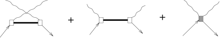
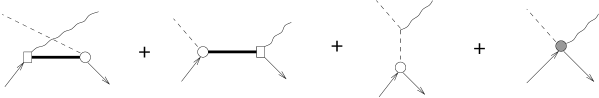
FIG. 1.: The tree-level diagrams including the contact terms contributing to the amplitude for Compton scattering (top) and pion photoproduction (bottom). The solid, dashed and wavy lines are nucleons, pions and photons, respectively. The thick line is the dressed nucleon propagator. The empty circle (square) is the dressed $\pi NN$ ($\gamma NN$)-vertex, and the shaded circle stands for the “contact” vertices. All the external lines are on-shell.

FIG. 2.: The Feynman diagrams forming the K-matrix for Compton scattering up to second order in the “potential” $V_{c^{\prime}c}$, according to Eq. (6). All the external lines are on-shell. The label Re shows that only the principal-value part of the loop integrals are included. The structure of the loop diagrams is labeled in terms of the tree diagrams for pion photoproduction, ss, su, st etc.

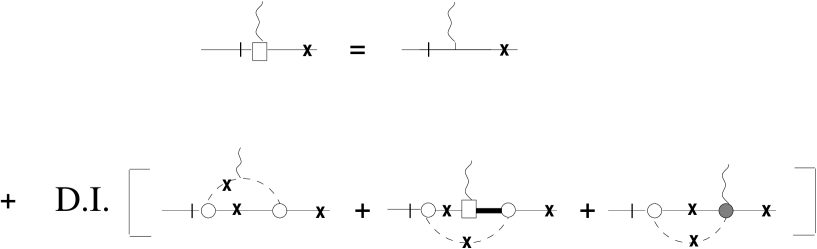
FIG. 3.: The graphical representation of Eq. (9) following the notation of Fig. (1). Crosses denote cut propagators and cut external lines are stripped away.

FIG. 4.: The imaginary (the upper panel) and real (the lower panel) parts of the form factors $F_{1}^{+}$ (the solid curves) and $F_{1}^{-}$ (the dotted curves) as functions of the momentum squared of the off-shell proton.

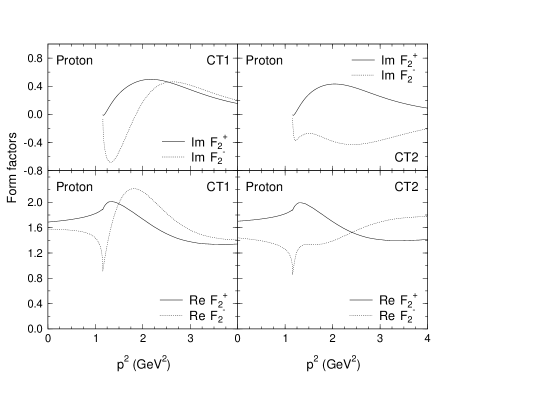
FIG. 5.: The same as Fig. (4), but for the form factors $F_{2}^{\pm}$ for two different using $\gamma\pi NN$-contact terms, Eq. (28) (left panel) and Eq. (C8) (right panel).

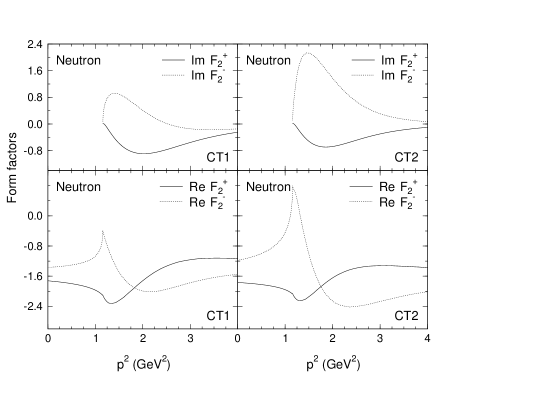
FIG. 6.: The same as in Fig. (5), but for the neutron-photon vertex.

FIG. 7.: The $f_{EE}^{1-}$ partial wave amplitude as function of the photon energy. The solid line represents the calculation where the dressed (irreducible) nucleon-photon, nucleon-pion vertices and the dressed nucleon propagator, are included in the K-matrix. The dashed line is the calculation where the bare vertices and the free nucleon propagator are used. The dotted curve is the result based on an analysis of pion-photoproduction data[2].

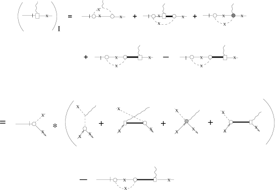
FIG. 8.: The diagrammatic equation for the pole contribution to the $\gamma NN$-vertex (indicated by the subscript I) as used in the proof of the consistency of the method with the Ward-Takahashi identity. The notation is as in Fig. (1). The asterisk denotes an integration over the phase space of the cut nucleon and pion lines.

REFERENCES

- [1] S. Kondratyuk and O. Scholten, Phys. Rev. C 59, 1070 (1999).
- [2] J. C. Bergstrom and E. L Hallin, Phys. Rev. C 48, 1508 (1993).
- [3] A.I. L’vov, V.A. Petrun’kin and M. Schumacher, Phys. Rev. C 55, 359 (1997).
- [4] A. Hünger, J. Peise, A. Robbiano et al., Nucl. Phys. A 62, 385 (1997).
- [5] O. Hanstein, D. Drechsel and L. Tiator, Nucl. Phys. A632, 561 (1998); D. Drechsel, O. Hanstein, S.S. Kamalov and L. Tiator, Nucl. Phys. A645, 145 (1999); D. Drechsel, M. Gorchtein, B. Pasquini and M. Vanderhaeghen, Phys. Rev. C 61, 015204 (2000).
- [6] A. Bincer, Phys. Rev. 118, 855 (1960); S. D. Drell and H. R. Pagels, Phys. Rev. 140, B397 (1965); E. M. Nyman, Nucl. Phys. A154, 97 (1970); M. G. Hare, Ann. Phys. (N.Y.) 74, 595 (1972).
- [7] H. W. L. Naus and J. H. Koch, Phys. Rev. C 36, 2459 (1987); P. C. Tiemeijer and J. A. Tjon, Phys. Rev. C 42, 599 (1990); J. W. Bos, S. Scherer and J. H Koch, Nucl. Phys. A547, 488 (1992); J. W. Bos and J. H. Koch, Nucl. Phys. A563, 539 (1993); X. Song, J.P. Chen and J.S. McCarthy, Z. Phys. A341, 275 (1992); H. C. Dönges, M. Schäfer and U. Mosel, Phys. Rev. C 51, 950 (1995).
- [8] E. M. Nyman, Nucl. Phys. A 160, 517 (1971). S. Kondratyuk, G. Martinus and O. Scholten, Phys. Lett. B 418, 20 (1998); Yi Li, M. K. Liou and W. M. Schreiber, Phys. Rev. C 57, 507 (1998).
- [9] A. Yu. Korchin, O. Scholten and F. de Jong, Phys. Lett. B 402, 1 (1997).
- [10] L. D. Landau, Nucl. Phys. 13, 181 (1959); S. Mandelstam, Phys. Rev. 115, 1741 (1959); R. E. Cutkosky, J. Math. Phys. 1, 429 (1960); G. ’t Hooft and M. J. G. Veltman, Diagrammar, CERN Yellow Report 73-09.
- [11] P.F.A. Goudsmit, H. J. Leisi, E. Matsinos, B. L. Birbrair, and A. B. Gridnev, Nucl. Phys. A575, 673 (1994).
- [12] O. Scholten, A. Yu. Korchin, V. Pascalutsa, and D. Van Neck, Phys. Lett. B 384, 13 (1996).
- [13] A.Yu. Korchin, O. Scholten, and R. G. E. Timmermans, Phys. Lett. B 438, 1 (1998).
- [14] K. Ohta, Phys. Rev. C 40, 1335 (1989).
- [15] F. Gross and D. O. Riska, Phys. Rev. C 36, 1928 (1987); H. Haberzettl, Phys. Rev. C 56, 2041 (1997); S.I. Nagorny and A. E. L. Dieperink, nucl-th/9803007.
- [16] J.D. Bjorken and S.D. Drell, Relativistic Quantum Mechanics, McGraw-Hill, 1964.
- [17] S. Kamefuchi, L. O’Raifeartaigh and A. Salam, Nucl. Phys. 28, 529 (1961); J.S.R. Chisholm, Nucl. Phys. 26, 469 (1961); G. Barton, Introduction to Advanced Field Theory, Interscience Publishers, 1963.
- [18] S. Scherer and H.W. Fearing, Phys. Rev. C 51, 359 (1995); H.W. Fearing, Phys. Rev. Lett. 81, 758 (1998); R.M. Davidson and G. I. Poulis, Phys. Rev. D 54, 2228 (1996).
- [19] V. Bernard, N. Kaiser, U. Meissner, Int. J. Mod. Phys. E4, 193 (1995).
- [20] REDUCE user’s manual, version 3.1, ed. A.C. Hearn, The Rand Corporation, Santa Monica, 1984.