Equilibration within a semiclassical off-shell transport approach

Abstract

Equilibration times for nuclear matter configurations – modelling intermediate and high energy nucleus-nucleus collisions – are evaluated within the semiclassical off-shell transport approach developed recently. The transport equations are solved for a finite box in coordinate space employing periodic boundary conditions. The off-shell transport model is shown to give proper off-shell equilibrium distributions in the limit $t\rightarrow\infty$ for the nucleon and $\Delta$-resonance spectral functions. We find that equilibration times within the off-shell approach are only slightly enhanced as compared to the on-shell limit for the momentum configurations considered.

PACS: 24.10.Cn; 24.10.-i; 25.70.-z
Keywords: Many-body theory; Nuclear-reaction models and methods; Low and intermediate energy heavy-ion reactions

1 Introduction

The dynamical description of strongly interacting systems out of equilibrium nowadays is dominantly based on transport theories and efficient numerical recipies have been set up for the solution of the coupled channel transport equations [1, 2] (and Refs. therein). These transport approaches have been derived either from the Kadanoff-Baym equations [3] in Refs. [4, 5, 6, 7, 8] or from the hierarchy of connected equal-time Green functions [9, 10] in Refs. [11, 12] by applying a Wigner transformation and restricting to first order in the derivatives of the phase-space variables ($X,P$). Whereas theoretical formulations of off-shell quantum transport have been limited to the formal level for a couple of years [5, 7, 13, 14] only recently a tractable semiclassic form has been derived for testparticles in the eight dimensional phase space of a particle [15, 16, 17].

Whereas in Refs. [15, 16] we have investigated the off-shell transport approach with respect to nucleus-nucleus collisions at GANIL, SIS and AGS energies, we here concentrate on equilibration phenomena relative to the on-shell dynamics by imposing periodic boundary conditions for the system confined to a box of size $V=L^{3}$, where $L$ denotes the length of the cubic box. We, furthermore, compare the equilibrium nucleon and $\Delta$ distribution functions ($t\rightarrow\infty$) to the statistical model (SM) employing the same spectral functions as in the transport approach. For related studies at higher bombarding energies or energy densities within on-shell transport approaches we refer the reader to Refs. [18, 19, 20, 21, 22].

2 Extended semiclassical transport equations

We briefly recall the basic equations for Green functions and particle self energies that are exploited in the derivation of off-shell transport equations in the semiclassical limit.

The general starting point for the derivation of a transport equation for particles with a finite and dynamical width are the Dyson-Schwinger equations for the retarded and advanced Green functions $S^{ret}$, $S^{adv}$ and for the non-ordered Green functions $S^{<}$ and $S^{>}$ [3]. In the case of scalar bosons – which is considered in the following for simplicity – these Green functions are defined by

$$\hskip 56.9055pti\,S^{<}_{xy} := \;<\,\Phi^{\dagger}(y)\;\Phi(x)\,>\,,\;\;i\,S^{>}_{xy}:=\;<\,\Phi(x)\;\Phi^{\dagger}(y)\,>\,,$$

$$i\,S^{ret}_{xy} := \phantom{-}\>\Theta(x_{0}-y_{0})\,<\,[\,\Phi(x)\,,\,\Phi^{\dagger}(y)\,]\,>\,,$$

$$i\,S^{adv}_{xy} := -\>\Theta(y_{0}-x_{0})\,<\,[\,\Phi(x)\,,\,\Phi^{\dagger}(y)\,]\,>\,.$$ (1)

They depend on the space-time coordinates $x,y$ as indicated by the indices $\cdot_{xy}$. The Green functions are determined via Dyson-Schwinger equations by the retarded and advanced self energies $\Sigma^{ret},\Sigma^{adv}$ and the collisional self energy $\Sigma^{<}$:

$$\hat{S}_{0x}^{-1}\;S_{xy}^{ret}\;\>=\;\>\delta_{xy}\;\>+\;\>\Sigma_{xz}^{ret}\>\odot\>S_{zy}^{ret}\;,$$ (2)

$$\hat{S}_{0x}^{-1}\;S_{xy}^{adv}\;\>=\;\>\delta_{xy}\;\>+\;\>\Sigma_{xz}^{adv}\>\odot\>S_{zy}^{adv}\;,$$ (3)

$$\hat{S}_{0x}^{-1}\;S_{xy}^{<}\;\>=\;\>\Sigma_{xz}^{ret}\>\odot\>S_{zy}^{<}\;\>+\;\>\Sigma_{xz}^{<}\>\odot\>S_{zy}^{adv}\>,$$ (4)

where Eq. (4) is the well-known Kadanoff-Baym equation. Here $\hat{S}^{-1}_{0x}$ denotes the (negative) Klein-Gordon differential operator which is given for bosonic field quanta of (bare) mass $M_{0}$ by $\hat{S}^{-1}_{0x}=-(\partial^{\mu}_{x}\partial^{x}_{\mu}+M^{2}_{0})$; $\delta_{xy}$ represents the four-dimensional $\delta$-distribution $\delta_{xy}\equiv\delta^{(4)}(x-y)$ and the symbol $\odot$ indicates an integration (from $-\infty$ to $\infty$) as well as a summation over all discrete intermediate variables (cf. [7, 15]).

2.1 The semiclassical limit

For the derivation of a semiclassical transport equation one now changes from a pure space-time formulation into the Wigner-representation. The theory is then formulated in terms of the center-of-mass variable $X=(x+y)/2$ and the momentum $P$, which is introduced by Fourier-transformation with respect to the relative space-time coordinate $(x-y)$. In any semiclassical transport theory one, furthermore, keeps only contributions up to the first order in the space-time gradients. After carrying-out these two steps the Dyson-Schwinger equations (2)-(4) become

$$\left[\,P^{2}\,-\,M^{2}_{0}\,+\,iP^{\mu}\partial^{X}_{\mu}\,\right]\>S^{ret}_{XP}\;=\;1\>+\>(\,1\,-\,i\,\Diamond\,)\,\{\,\Sigma^{ret}_{XP}\,\}\>\{\,S^{ret}_{XP}\,\}\>,$$ (5)

$$\left[\,P^{2}\,-\,M^{2}_{0}\,+\,iP^{\mu}\partial^{X}_{\mu}\,\right]\>S^{adv}_{XP}\;=\;1\>+\>(\,1\,-\,i\,\Diamond\,)\,\{\,\Sigma^{adv}_{XP}\,\}\>\{\,S^{adv}_{XP}\,\}\>,$$ (6)

$$\left[\,P^{2}\,-\,M^{2}_{0}\,+\,iP^{\mu}\partial^{X}_{\mu}\,\right]\>S^{<}_{XP}\;=\;(\,1\,-\,i\,\Diamond\,)\,\left[\>\{\,\Sigma^{ret}_{XP}\,\}\>\{\,S^{<}_{XP}\,\}\;+\;\{\,\Sigma^{<}_{XP}\,\}\>\{\,S^{adv}_{XP}\,\}\>\right],$$ (7)

where the operator $\Diamond$ is defined as [7, 15]

$$\Diamond\,\{\,F_{1}\,\}\,\{\,F_{2}\,\}\;:=\;\frac{1}{2}\left(\frac{\partial F_{1}}{\partial X^{\mu}}\>\frac{\partial F_{2}}{\partial P_{\mu}}\;-\;\frac{\partial F_{1}}{\partial P_{\mu}}\>\frac{\partial F_{2}}{\partial X^{\mu}}\right).$$ (8)

It is a four-dimensional generalization of the well-known Poisson-bracket. Starting from (5) and (6) one obtains algebraic relations between the real and the imaginary part of the retarded Green functions. On the other hand eq. (7) leads to a ’transport equation’ for the Green function $S^{<}$ [15].

To this aim one separates all retarded and advanced quantities – Green functions and self energies – into real and imaginary parts,

$$S_{XP}^{ret,adv}\;=\;ReS^{ret}_{XP}\;\mp\;\frac{i}{2}\,A_{XP}\;,\qquad\Sigma_{XP}^{ret,adv}\;=\;Re\Sigma^{ret}_{XP}\;\mp\;\frac{i}{2}\,\Gamma_{XP}\;.$$ (9)

The imaginary part of the retarded propagator is given (up to a factor 2) by the normalized spectral function

$$A_{XP}\>=\>i\left[\,S_{XP}^{ret}\>-\>S_{XP}^{adv}\,\right]\>=\>-2\,Im\,S^{ret}_{XP}\;,\qquad\qquad\qquad\int\frac{dP_{0}^{2}}{4\pi}\,A_{XP}\;=\;1\;,$$ (10)

while the imaginary part of the self energy corresponds to half the particle width $\Gamma_{XP}$. By separating the complex equations (5) and (6) into their real and imaginary contributions we obtain an algebraic equation between the real and the imaginary part of $S^{ret}$,

$$ReS^{ret}_{XP}\;=\;\frac{P^{2}\>-\>M_{0}^{2}\>-\>Re\Sigma^{ret}_{XP}}{\Gamma_{XP}}\;A_{XP}\,.$$ (11)

In addition we gain an algebraic solution for the spectral function as

$$A_{XP}\;=\;\frac{\Gamma_{XP}}{(\,P^{2}\,-\,M_{0}^{2}\,-\,Re\Sigma^{ret}_{XP})^{2}\>+\>\Gamma_{XP}^{2}/4}\;,$$ (12)

while the real part of the retarded propagator is given by

$$ReS^{ret}_{XP}\;=\;\frac{P^{2}\>-\>M_{0}^{2}\>-\>Re\Sigma^{ret}_{XP}}{(\,P^{2}\,-\,M_{0}^{2}\,-\,Re\Sigma^{ret}_{XP})^{2}\>+\>\Gamma_{XP}^{2}/4}\,.$$ (13)

Furthermore, the (Wigner-transformed) Kadanoff-Baym equation (7) allows for the construction of a transport equation for the Green function $S^{<}$. When separating the real and the imaginary contribution of this equation we find i) a generalized transport equation,

$$\Diamond\,\{\,P^{2} - M_{0}^{2}\>-\>Re\Sigma^{ret}_{XP}\,\}\;\{\,S^{<}_{XP}\,\}\;-\;\Diamond\,\{\,\Sigma^{<}_{XP}\,\}\;\{ReS^{ret}_{XP}\,\}$$ (14)

$$= \frac{i}{2}\>\left[\>\Sigma^{>}_{XP}\>S^{<}_{XP}\;-\;\Sigma^{<}_{XP}\>S^{>}_{XP}\>\right],$$

and ii) a generalized mass-shell constraint

$$[\,P^{2} - M_{0}^{2}\>-\>Re\Sigma^{ret}_{XP}\,]\;S^{<}_{XP}\;-\;\Sigma^{<}_{XP}\;ReS^{ret}_{XP}$$ (15)

$$= \frac{1}{2}\,\Diamond\;\{\,\Sigma^{<}_{XP}\,\}\;\{\,A_{XP}\,\}\;-\;\frac{1}{2}\,\Diamond\;\{\,\Gamma_{XP}\,\}\;\{\,S^{<}_{XP}\,\}\;.$$

Besides the drift term (i.e. $\Diamond\{P^{2}-M^{2}_{0}\}\{S^{<}\}=-P^{\mu}\partial^{X}_{\mu}S^{<})$ and the Vlasov term (i.e. $-\Diamond\{Re\Sigma^{ret}\}\{S^{<}\}$) a third contribution appears on the l.h.s. of (14) (i.e. $-\Diamond\{\Sigma^{<}\}\{ReS^{ret}\}$), which vanishes in the quasiparticle limit and incorporates – as shown in [15, 16, 17] – the off-shell behaviour in the particle propagation which has been neglected so far in transport studies. The r.h.s. of (14) consists of a collision term with its characteristic gain ($\sim\Sigma^{<}S^{>}$) and loss ($\sim\Sigma^{>}S^{<}$) structure, where scattering and decay processes of particles are described.

Within the specific term ($\Diamond\{\Sigma^{<}\}\{ReS^{ret}\}$) a further modification is necessary. According to Botermans and Malfliet [5] the collisional self energy $\Sigma^{<}$ should be replaced by $S^{<}\cdot\Gamma/A$ to gain a consistent first order gradient expansion scheme. The replacement is allowed since the difference between these two expressions $(\Sigma^{<}-S^{<}\cdot\Gamma/A)$ can be shown to be of first order in the space-time gradients itself [15]. Furthermore, this substitution is required to get rid of the inequivalence between the general transport equation (14) and the general mass shell constraint (15) [25].

Finally, the general transport equation (in first order gradient expansion) reads [15, 16, 17]

$$A_{XP}\,\Gamma_{XP} \!\!\!\!\!\!\!\!\!\!\left[\,\Diamond\;\{\,P^{2}-M_{0}^{2}-Re\Sigma^{ret}_{XP}\,\}\;\{\,S^{<}_{XP}\,\}\>-\>\frac{1}{\Gamma_{XP}}\;\Diamond\;\{\,\Gamma_{XP}\,\}\;\{\,(\,P^{2}-M_{0}^{2}-Re\Sigma^{ret}_{XP}\,)\,S^{<}_{XP}\,\}\,\right]$$ (16)

$$\;=\;i\,\left[\,\Sigma^{>}_{XP}\>S^{<}_{XP}\>-\>\Sigma^{<}_{XP}\>S^{>}_{XP}\,\right].$$

Its formal structure is fixed by the approximations applied, however, its physical contents is fully determined by the different self energies, i.e. $Re\Sigma_{XP}^{ret},\Gamma_{XP},\Sigma_{XP}^{<}$ that have to be specified in addition.

In order to obtain an approximate solution to the transport equation (16) a testparticle ansatz is used for the Green function $S^{<}$, more specifically for the real and positive semidefinite quantity $F_{XP}\;=A_{XP}N_{XP}=\;i\,S^{<}_{XP}$,

$$F_{XP}\;\sim\;\sum_{i=1}^{N}\;\delta^{(3)}({\vec{X}}\,-\,{\vec{X}}_{i}(t))\;\;\delta^{(3)}({\vec{P}}\,-\,{\vec{P}}_{i}(t))\;\;\delta(P_{0}-\,\epsilon_{i}(t))\>.$$ (17)

In the most general case (where the self energies depend on four-momentum $P$, time $t=X_{0}$ and the spatial coordinates $\vec{X}$) the equations of motion for the testparticles read [16]

$$\frac{d{\vec{X}}_{i}}{dt}\! = \!\phantom{-}\frac{1}{1-C_{(i)}}\,\frac{1}{2\epsilon_{i}}\>\left[\,2\,{\vec{P}}_{i}\,+\,{\vec{\nabla}}_{P_{i}}\,Re\Sigma^{ret}_{(i)}\,+\,\frac{\epsilon_{i}^{2}-{\vec{P}}_{i}^{2}-M_{0}^{2}-Re\Sigma^{ret}_{(i)}}{\Gamma_{(i)}}\>{\vec{\nabla}}_{P_{i}}\,\Gamma_{(i)}\>\right],$$ (18)

$$\frac{d{\vec{P}}_{i}}{dt}\! = \!-\frac{1}{1-C_{(i)}}\,\frac{1}{2\epsilon_{i}}\>\left[{\vec{\nabla}}_{X_{i}}\,Re\Sigma^{ret}_{i}\>+\>\frac{\epsilon_{i}^{2}-{\vec{P}}_{i}^{2}-M_{0}^{2}-Re\Sigma^{ret}_{(i)}}{\Gamma_{(i)}}\>{\vec{\nabla}}_{X_{i}}\,\Gamma_{(i)}\>\right],$$ (19)

$$\frac{d\epsilon_{i}}{dt}\! = \!\phantom{-}\frac{1}{1-C_{(i)}}\,\frac{1}{2\epsilon_{i}}\>\left[\frac{\partial Re\Sigma^{ret}_{(i)}}{\partial t}\>+\>\frac{\epsilon_{i}^{2}-{\vec{P}}_{i}^{2}-M_{0}^{2}-Re\Sigma^{ret}_{(i)}}{\Gamma_{(i)}}\>\frac{\partial\Gamma_{(i)}}{\partial t}\right],$$ (20)

where the notation $F_{(i)}$ implies that the function is taken at the coordinates of the testparticle, i.e. $F_{(i)}\equiv F(t,\vec{X}_{i}(t),\vec{P}_{i}(t),\epsilon_{i}(t))$.

In (18-20) a common multiplication factor $(1-C_{(i)})^{-1}$ appears, which contains the energy derivatives of the retarded self energy

$$C_{(i)}\>=\>\frac{1}{2\epsilon_{i}}\left[\frac{\partial}{\partial\epsilon_{i}}\,Re\Sigma^{ret}_{(i)}\>+\>\frac{\epsilon_{i}^{2}-{\vec{P}}_{i}^{2}-M_{0}^{2}-Re\Sigma^{ret}_{(i)}}{\Gamma_{(i)}}\>\frac{\partial}{\partial\epsilon_{i}}\,\Gamma_{(i)}\right]\>,$$ (21)

which yields a shift of the system time $t$ to the ’eigentime’ of particle $i$ defined by $\tilde{t}_{i}=t/(1-C_{(i)})$. The derivatives with respect to the ’eigentime’, i.e. $d\vec{X}_{i}/d\tilde{t}_{i}$, $d\vec{P}_{i}/d\tilde{t}_{i}$ and $d\epsilon_{i}/d\tilde{t}_{i}$ then emerge without this renormalization factor for each testparticle $i$ when neglecting the explicit time dependence of $C_{(i)}$ in line with the semiclassical approximation scheme. The role and the importance of this correction factors have been studied in Ref. [16] for a four-momentum-dependent ’trial’ potential and we refer the reader to the latter analysis for more details.

Following Ref. [15] we take $M^{2}=P^{2}-Re\Sigma^{ret}$ as an independent variable instead of the energy $P_{0}$. Eq. (20) then turns to

$$\frac{dM_{i}^{2}}{dt}\;=\;\frac{M_{i}^{2}-M_{0}^{2}}{\Gamma_{(i)}}\;\frac{d\Gamma_{(i)}}{dt}$$ (22)

for the time evolution of the test-particle $i$ in the invariant mass squared as derived in Refs. [15, 16]. We mention that corresponding equations of motion have been derived by Leupold in the nonrelativistic limit [17].

2.2 Generalized collision terms for bosons and fermions

The collision term of the Kadanoff-Baym equation can only be worked out in more detail by giving explicit approximations for $\Sigma^{<}$ and $\Sigma^{>}$. We recall the formulation and result from Ref. [16] that is based on Dirac-Brueckner theory, i.e.

$$I_{coll}(X,\vec{P},M^{2})=Tr_{2}Tr_{3}Tr_{4}A(X,{\vec{P}},M^{2})A(X,{\vec{P}}_{2},M_{2}^{2})A(X,{\vec{P}}_{3},M_{3}^{2})A(X,{\vec{P}}_{4},M_{4}^{2})$$

$$|T(({\vec{P}},M^{2})+({\vec{P}}_{2},M_{2}^{2})\rightarrow({\vec{P}}_{3},M_{3}^{2})+({\vec{P}}_{4},M_{4}^{2}))|_{{\cal A,S}}^{2}\;\;\delta^{(4)}({P}+{P}_{2}-{P}_{3}-{P}_{4})$$

$$\hskip 28.45274pt[\,N_{X{\vec{P}}_{3}M_{3}^{2}}\,N_{X{\vec{P}}_{4}M_{4}^{2}}\,{\bar{f}}_{X{\vec{P}}M^{2}}\,{\bar{f}}_{X{\vec{P}}_{2}M_{2}^{2}}\>-\>N_{X{\vec{P}}M^{2}}\,N_{X{\vec{P}}_{2}M_{2}^{2}}\,{\bar{f}}_{X{\vec{P}}_{3}M_{3}^{2}}\,{\bar{f}}_{X{\vec{P}}_{4}M_{4}^{2}}\,]$$ (23)

with

$${\bar{f}}_{X{\vec{P}}M^{2}}=1+\eta\,N_{X{\vec{P}}M^{2}}$$ (24)

and $\eta=\pm 1$ for bosons/fermions, respectively. The indices ${\cal A,S}$ stand for the antisymmetric/symmetric matrix element of the in-medium off-shell scattering amplitude $T$ in case of fermions/bosons. In Eq. (23) the trace over particles 2,3,4 reads explicitly for fermions

$$Tr_{2}=\sum_{\sigma_{2},\tau_{2}}\frac{1}{(2\pi)^{4}}\int d^{3}P_{2}\frac{dM^{2}_{2}}{2\sqrt{\vec{P}^{2}_{2}+M^{2}_{2}}},$$ (25)

where $\sigma_{2},\tau_{2}$ denote the spin and isospin of particle 2. In case of bosons we have instead

$$Tr_{2}=\sum_{\sigma_{2},\tau_{2}}\frac{1}{(2\pi)^{4}}\int d^{3}P_{2}\frac{dP_{0,2}^{2}}{2},$$ (26)

since here the spectral function $A_{B}$ is normalized as

$$\int\frac{dP_{0}^{2}}{4\pi}A_{B}(X,P)=1$$ (27)

whereas for fermions we have

$$\int\frac{dP_{0}}{2\pi}A_{F}(X,P)=1.$$ (28)

We mention that the spectral function $A_{F}$ in case of fermions in (23) is obtained by considering only particles of positive energy and assuming the spectral function to be identical for spin ’up’ and ’down’ states (cf. Ref. [16]).

Neglecting the ’gain-term’ in Eq. (23) one recognizes that the collisional width $\Gamma_{coll}$ of the particle in the rest frame is given by

$$\Gamma_{coll}(X,\vec{P},M^{2})=Tr_{2}Tr_{3}Tr_{4}\;|T(({\vec{P}},M^{2})+({\vec{P}}_{2},M_{2}^{2})\rightarrow({\vec{P}}_{3},M_{3}^{2})+({\vec{P}}_{4},M_{4}^{2}))|_{{\cal A,S}}^{2}$$ (29)

$$A(X,{\vec{P}}_{2},M_{2}^{2})A(X,{\vec{P}}_{3},M_{3}^{2})A(X,{\vec{P}}_{4},M_{4}^{2})\;\;\delta^{4}(P+P_{2}-P_{3}-P_{4})\ N_{X{\vec{P}}_{2}M_{2}^{2}}\,{\bar{f}}_{X{\vec{P}}_{3}M^{2}_{3}}\,{\bar{f}}_{X{\vec{P}}_{4}M^{2}_{4}}\,,$$

where as in Eq. (23) local off-shell transition amplitudes enter for the transitions $P+P_{2}\rightarrow P_{3}+P_{4}$. We note that the extension of Eq. (23) to inelastic scattering processes (e.g. $NN\rightarrow N\Delta$) or ($\pi N\rightarrow\Delta$ etc.) is straightforward when exchanging the elastic transition amplitude $T$ by the corresponding inelastic one and taking care of Pauli-blocking or Bose-enhancement for the particles in the final state. The relation of the quantity $\Gamma_{XP}$ to the collisional width $\Gamma_{coll}$ is given by $\Gamma_{XP}=2P_{0}(\Gamma_{decay}(XP)+\Gamma_{coll}(XP))$, where the particle decay width $\Gamma_{decay}$ in the medium might also be different compared to the vacuum.

Thus the transport approach determines the particle spectral function dynamically via (29) – with respect to the collisional width $\Gamma_{coll}$ – for all hadrons if the in-medium transition amplitudes $T$ are known in their full off-shell dependence. Since this information is not available for configurations of hot and dense matter, a couple of assumptions and numerical approximation schemes have to be invoked in actual applications so far.

As in Refs. [15, 16] the following dynamical calculations are based on the conventional HSD transport approach [2, 26] – in which $Re\Sigma^{ret}_{XP}$ is specified for the hadrons – however, the equations of motion for the testparticles are extended to (18,19,22). For further details on the elastic and inelastic transition rates we refer the reader to Ref. [16].

2.3 Comment on particle number conservation

In previous derivations of the off-shell transport equations one has started from a formulation of the non-equilibrium theory in space-time representation $(x,x^{\prime})$ and then changed into a phase-space representation via Fourier transformation with respect to $(x-x^{\prime})$ [5, 15, 16, 17]. The semiclassical limit then has been introduced by assuming gradients in $X=(x+x^{\prime})/2$ to be small [17] for $Re\Sigma^{ret}_{XP}$ and $S^{<}_{XP}$. Here we argue that for reasons of symmetry in phase-space also the four-momentum derivatives in $P$ have to be small to achieve a proper semiclassical limit as inherent in the formulation of the transport equation (16) in terms of the generalized Poisson-bracket (8).

We briefly demonstrate in the following lines that instead of a coordinate-space representation one may formulate the theory equivalently in momentum-space and then transform to phase space: The momentum-dependent (two-point) functions are given as

$$F_{p_{1\phantom{{}^{\prime}}\!\!}\,p_{1^{\prime}}}\>=\>\int\!d^{4}\!x_{1}\!\int d^{4}\!x_{1^{\prime}}\;\;e^{i(p_{1\phantom{{}^{\prime}}\!\!}x_{1\phantom{{}^{\prime}}\!\!}-\,p_{1^{\prime}}x_{1^{\prime}})}\;\;F_{x_{1\phantom{{}^{\prime}}\!\!}\,x_{1^{\prime}}}.$$ (30)

The evolution of the retarded and advanced Green functions $S^{ret},S^{adv}$ and the Green function $S^{<}$ turns to

$$\hat{S}_{0\,p_{1\phantom{{}^{\prime}}\!\!}}^{-1}\;S_{p_{1\phantom{{}^{\prime}}\!\!}\,p_{1^{\prime}}}^{ret,adv}\; = \>(2\pi)^{4}\;\delta^{(4)}(p_{1\phantom{{}^{\prime}}\!\!}-p_{1^{\prime}})\;\>+\>\>\int\frac{d^{4}p_{2}}{(2\pi)^{4}}\;\;\Sigma_{p_{1\phantom{{}^{\prime}}\!\!}\,p_{2\phantom{{}^{\prime}}\!\!}}^{ret,adv}\;\;S_{p_{2\phantom{{}^{\prime}}\!\!}\,p_{1^{\prime}}}^{ret,adv}\;,$$ (31)

$$\hat{S}_{0\,p_{1\phantom{{}^{\prime}}\!\!}}^{-1}\;S_{p_{1\phantom{{}^{\prime}}\!\!}\,p_{1^{\prime}}}^{<}\; = \>\int\frac{d^{4}p_{2}}{(2\pi)^{4}}\;\;\left[\;\Sigma_{p_{1\phantom{{}^{\prime}}\!\!}\,p_{2\phantom{{}^{\prime}}\!\!}}^{ret}\;S_{p_{2\phantom{{}^{\prime}}\!\!}\,p_{1^{\prime}}}^{<}\;\>+\;\>\Sigma_{p_{1\phantom{{}^{\prime}}\!\!}\,p_{2\phantom{{}^{\prime}}\!\!}}^{<}\;\ S_{p_{2\phantom{{}^{\prime}}\!\!}\,p_{1^{\prime}}}^{adv}\;\right]\>,$$ (32)

with the ’kinetic’ operator in momentum-space $\hat{S}_{0\,p_{1}}^{-1}=(p_{1}^{2}-M^{2}_{0})$ in the case of relativistic scalar bosons with (bare) mass $M_{0}$. Obviously, the equations in momentum-space are formally equivalent to the equations in coordinate-space, i.e. the convolution integrals in the coordinate $x_{2}$ are replaced by convolution integrals in the momentum $p_{2}$. When transforming from momentum- to phase-space via a Fourier-transformation with respect to the four-momentum coordinate $(p_{1}-p_{1^{\prime}})$

$$F_{XP}\>=\>\int\frac{d^{4}(p_{1}\!-\!p_{1^{\prime}})}{(2\pi)^{4}}\;\;e^{-iX(p_{1\phantom{{}^{\prime}}\!\!}-p_{1^{\prime}})}\;\;F_{p_{1\phantom{{}^{\prime}}\!\!}\,p_{1^{\prime}}}$$ (33)

(with $P=(p_{1}+p_{1^{\prime}})/2$) we gain again the familiar equations in Wigner-representation:

$$\hat{S}_{0\,XP}^{-1}\;S_{XP}^{ret,adv}\; = \;1\;\>+\>\>e^{-i\Diamond}\;\;\Sigma_{XP}^{ret,adv}\;S_{XP}^{ret,adv}$$ (34)

$$\hat{S}_{0\,XP}^{-1}\;S_{XP}^{<}\; = \>e^{-i\Diamond}\;\left[\;\Sigma_{XP}^{ret}\;\;S_{XP}^{<}\;\>+\;\>\Sigma_{XP}^{<}\;\;S_{XP}^{adv}\;\right]\>,$$ (35)

with the ’kinetic’ operator in phase-space $\hat{S}_{0\,XP}^{-1}=(P^{2}+iP^{\mu}\partial^{X}_{\mu}-\frac{1}{4}\partial^{X}_{\mu}\partial_{X}^{\mu}-M^{2}_{0})$. Here we have used the following relation for the convolution integrals in momentum-space

$$\int\frac{d^{4}(p_{1}\!-\!p_{1^{\prime}})}{(2\pi)^{4}}\;\;e^{-iX(p_{1}-p_{1^{\prime}})}\;\int\frac{d^{4}p_{2}}{(2\pi)^{4}}\;\;\;F_{1,\,p_{1\phantom{{}^{\prime}}\!\!}\,p_{2\phantom{{}^{\prime}}\!\!}}\;F_{2,\,p_{2\phantom{{}^{\prime}}\!\!}\,p_{1^{\prime}}}\;\;=\;\;e^{-i\Diamond}\;\;F_{1,\,PX}\;\;F_{2,\,PX},$$ (36)

with the Poisson-operator $\Diamond$ defined in (8).

The semiclassical limit – along the conventional line of arguments – now is achieved by assuming gradients of the self energies $\Sigma^{ret,adv}$ in $P$ to be small. This assumption is especially well taken for systems with dominantly short range interactions since the different self energies $\Sigma^{ret,adv}(p,p^{\prime})$ become smooth functions in momentum-space such that a restriction to first order gradients in the momentum $P=(p+p^{\prime})/2$ can be more easily justified. Note again that the four-dimensional Poisson-bracket (8) is symmetric in the space-time and the four-momentum derivatives. Thus a phase-space gradient expansion requires all gradients to be small contrary to the assumptions made in Ref. [17].

As a consequence mixed gradients of second order as $\partial^{2}/(\partial t\partial p_{0})$ have to be neglected in a consistent truncation scheme of first order. As shown by Botermans and Malfliet in the review [5] the particle number conservation then holds strictly. Only when keeping special terms of second order $(\sim\partial^{2}/(\partial t\partial p_{0})$ unphysical pecularities may appear, that lead to a violation of particle number conservation in contradiction to the full theory (2)-(4).

3 Infinite nuclear matter problems

In case of infinite nuclear matter problems the solution of the transport equations simplifies since all spatial gradients (with respect to $\vec{X}$) vanish. This implies that the momentum coordinates of the testparticles $\vec{P}_{i}$ are constant according to (19) in between collisions.

The initial conditions of the problem then are fully specified by an initial bombarding energy per nucleon, that defines the relative shift in momentum of two Fermi spheres with a Fermi momentum $P_{F}$ = 260 MeV/c, the number of nucleons $N$ and the total volume of the box $V=L^{3}$. Alternatively, one can also characterize the system by an average density $\rho=N/V$ and energy density $\epsilon$ (cf. Ref. [18]). We use $L=10$ fm and assume an equal number of neutrons and protons.

In general (for $t\rightarrow\infty$) the stationary solution of Eq. (23) for a fermion $h$ is given by

$$F_{h}(\vec{X},\vec{P},M^{2})\;=\;\frac{A_{h}({\vec{X}},{\vec{P}},M^{2})}{\exp((E-\mu_{h})/T)-\eta}$$ (37)

with $E=\sqrt{{\vec{P}}^{2}+M^{2}}$ and $\eta=\pm 1$ for bosons/fermions, respectively, while $A_{h}$ denotes the spectral function (12), $T$ the temperature of the system and $\mu_{h}$ the chemical potential for the hadron. This situation corresponds to the grand canonical ensemble of quantum statistical mechanics. In case of infinite nuclear matter problems the dependence on $\vec{X}$ vanishes additionally.

3.1 Numerical results

As an example for equilibration phenomena we show in Fig. 1 the time evolution of the quadrupole moment (involving all baryons $B$)

$$Q_{2}(t)=\sum_{B}\frac{g_{B}}{(2\pi)^{4}}\int d^{3}X\int d^{3}P\,\frac{dM^{2}}{2\sqrt{{\vec{P}}^{2}+M^{2}}}\ (2P_{z}^{2}-P_{x}^{2}-P_{y}^{2})\ F_{B}(\vec{X},t,\vec{P},M^{2}),$$ (38)

for $\rho=\rho_{0}$ and initial bombarding energies of 0.1 A GeV and 1 A GeV, respectively. In (38) the degeneracy factor is $g_{B}=4$ for nucleons and $g_{B}$= 16 for $\Delta$-resonances. The solid lines result from the off-shell calculation while the dashed lines result from the on-shell limit. As can be seen from Fig. 1 the off-shell results are practically identical to the on-shell limits except for the very long time behaviour, where the off-shell limit needs some more time to achieve equilibrium. However, when defining an equilibration time $\tau$ by a drop of the observable by the factor $e^{-1}$ we find no sizeable effect from the off-shell propagation on $\tau$.

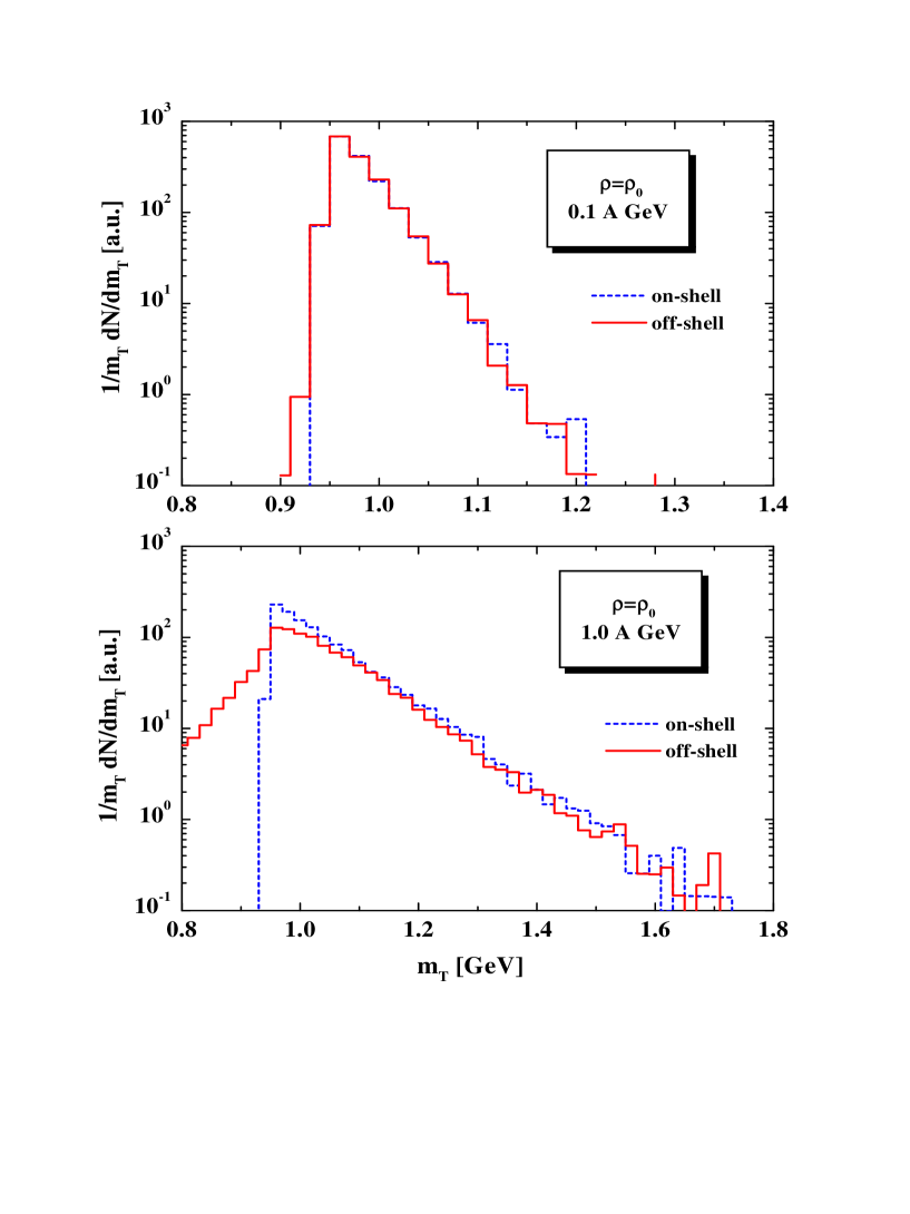
Figure 2: The transverse mass distribution for an infinite nuclear matter problem at bombarding energies of 0.1 A GeV (upper part) and 1 A GeV (lower part) at density $\rho=\rho_{0}$. The solid lines present the results for the off-shell calculations while the dashed lines are obtained in the on-shell limit.

The equilibrium distributions in the nucleon transverse mass $M_{t}=\sqrt{p_{t}^{2}+M^{2}}$ are shown in Fig. 2 for initial bombarding energies of 0.1 A GeV (upper part) and 1 A GeV (lower part). Again the solid lines denote the off-shell results from the transport calculations while the on-shell spectra are displayed in terms of dashed lines. Both limits (within the statistics) give the same temperature $T\approx$ 97 MeV for 1.0 A GeV and $T\approx$ 26 MeV for 0.1 A GeV as can be extracted from the high energy tail of the transverse mass spectra. Differences can only be found for $m_{T}\leq M_{0}$ since the finite width in the nucleon spectral function only can show up in the off-shell case. This component is quite small at 0.1 A GeV since the collisional width of nucleons at density $\rho_{0}$ and temperature $T\approx$ 26 MeV is about 8 MeV.

Without explicit display we mention that the time evolution of the nucleon spectral function in the invariant mass $M$ becomes broad in the initial nonequilibrium phase of the reaction and approaches the equilibrium distribution (37) roughly within the equilibration times from Fig. 1. Since the width of the nucleon spectral function in equilibrium at 0.1 A GeV (GANIL energy) is rather small ($\Gamma\approx$ 8 MeV) we concentrate on the energy of 1 A GeV (SIS energy) in the following, where the nucleon collisional width $\Gamma_{coll}$ at a temperature of 97 MeV is about 40 MeV and roughly 20% of the baryons are excited $\Delta$ resonances.

As demonstrated above, for the equilibrated system we can extract a temperature $T$ by fitting the particle spectra with the Bolzmann distribution

$${d^{3}N_{i}\over dp^{3}}\sim\exp(-E_{i}/T),$$ (39)

where $E_{i}=\sqrt{p_{i}^{2}+m_{i}^{2}}$ is the energy of particle $i$. We note that at the temperatures of interest here, the Bose and Fermi distributions are practically identical to a Boltzmann distribution. We find that in equilibrium the spectra of all particles (nucleons, $\Delta$’s and pions) can be characterized by a single temperature $T$ (cf. e.g. Ref. [18]).

3.2 Comparison to the statistical model

In order to investigate the equilibrium behaviour of hadron matter we compare our transport (box) calculations with a simple Statistical Model (SM) for an Ideal Hadron Gas where the system is described by a grand canonical ensemble of non-interacting fermions and bosons in equilibrium at temperature $T$. All baryon and meson species considered in the transport model ($N,\Delta,\pi$) also are included in the statistical model.

We recall that in the SM particle multiplicities $n_{i}$ and energy densities $\varepsilon_{i}$ for particles with spectral functions $A_{i}$ are given by

$$n_{i}={g_{i}\over(2\pi\hbar)^{3}}\int\frac{dM}{2\pi}\int\limits_{0}^{\infty}{A_{i}(M)/4\pi p^{2}dp\over\exp\left[(E_{i}-B_{i}\mu_{B}-S_{i}\mu_{S})/T\right]-\eta},$$ (40)

$$\varepsilon_{i}={g_{i}\over(2\pi\hbar)^{3}}\int\frac{dM}{2\pi}\int\limits_{0}^{\infty}{A_{i}(M)\ 4\pi E_{i}p^{2}dp\over\exp\left[(E_{i}-B_{i}\mu_{B}-S_{i}\mu_{S})/T\right]-\eta},$$ (41)

where $E_{i}=\sqrt{p^{2}+M^{2}}$ is the energy of particle $i$, $B_{i}$ is the baryon charge, $S_{i}$ is the strangeness, and $g_{i}$ is the spin-isospin degeneracy factor, while $\eta=\pm 1$ for bosons/fermions, respectively. In Eqs. (40),(41) $\mu_{B}$ and $\mu_{S}$ are the baryon and strangeness chemical potentials. The energy density $\varepsilon$, baryon density $\rho$ and strange particle density of the whole system in equilibrium then is given as

$$\varepsilon=\sum\limits_{i}\varepsilon_{i}(T,\mu_{B},\mu_{S})$$ (42)

$$\rho=\sum\limits_{i}B_{i}\ n_{i}(T,\mu_{B},\mu_{S})$$ (43)

$$\rho_{S}=\sum\limits_{i}S_{i}\ n_{i}(T,\mu_{B},\mu_{S})\,\equiv\,0.$$ (44)

As ’input’ for the SM we use the same $\varepsilon,\rho$ and $\rho_{S}$ as in the box calculations and we obtain the thermodynamical parameters – $T,\mu_{B},\mu_{S}$ – by solving the system of nonlinear equations (42),(43) and (44).

We now turn to a comparison of the equilibrium distributions in mass for nucleons and $\Delta$’s, i.e. $dN_{N}/dM$ and $dN_{\Delta}/dM$, from the box calculations with those from the SM, which are obtained by integration (summation) over momentum. We first discuss the on-shell limit where the nucleon spectral function is represented by a $\delta$-function around the bare mass while the $\Delta$ spectral function – as implemented in the transport approach – is given by (in the $\Delta$ rest frame)

$$A_{\Delta}(M)\;=\;\frac{2M^{2}\Gamma_{\pi N}(M)}{(M^{2}-M_{\Delta 0}^{2})^{2}+M^{2}\Gamma^{2}_{\pi N}(M)}$$ (45)

with

$$\Gamma_{\pi N}(M)=\Gamma_{0}(\frac{q}{q_{R}})^{3}\ (\frac{q_{R}^{2}+\delta^{2}}{q^{2}+\delta^{2}})^{3},$$ (46)

where $q_{R}$ denotes the pion momentum in the $\Delta$ rest frame of the resonance and $q$ is the corresponding pion three-momentum at invariant mass $M$, i.e.

$$q^{2}=\frac{(M^{2}-(M_{N}+M_{\pi})^{2})(M^{2}-(M_{N}-M_{\pi})^{2})}{4M^{2}}.$$ (47)

The quantity $\delta$ in (46) is fixed by [27]

$$\delta^{2}=(M-M_{N}-M_{\pi})^{2}+\frac{\Gamma_{0}^{2}}{4}$$ (48)

with $\Gamma_{0}=120$ MeV to achieve a good description for the $\pi N\rightarrow\Delta$ reaction in vacuum. Recall that in this case we have $\Gamma_{XP}/(2M)=\Gamma_{decay}=\Gamma_{\pi N}$ in the $\Delta$ rest frame, i.e. $\Gamma_{coll}$ = 0.

In the upper part of Fig. 3 we compare the asymptotic ($t\rightarrow\infty$) distributions for nucleons ($N$) and $\Delta$’s in the on-shell limit from the transport (box) calculation (solid histograms) with the result from the SM at a temperature $T$ = 97 MeV employing the $\Delta$ spectral function (45). Since the differences are hardly visible, we conclude that the transport calculation reproduces the result from the SM, where the thermodynamical parameters are determined by energy and baryon number conservation. We mention that we have discarded strangeness in this comparison, since kaons and hyperons are very scarce at this energy and have been switched off in both models. Since the $\Delta$ width (46) is zero below the $\pi N$ threshold, the $\Delta$ mass distribution only can extend above $M_{\pi}+M_{N}$.

In case of the off-shell calculation we obtain somewhat different mass distributions for nucleons and $\Delta$’s from the box calculation, which are given in terms of the solid histograms in the lower part of Fig. 3. Here the nucleon spectral function becomes very broad and also the $\Delta$ distribution extends below the $\pi N$ threshold in vacuum. The nucleon spectral function is broadened due to the elastic ($NN\rightarrow NN$) and inelastic ($NN\rightarrow N\Delta$) scattering processes, which can roughly be described by a collisional width $\Gamma_{coll}$ of 40 MeV in the nucleon spectral function

$$A_{N}(M)\;=\;\frac{2M^{2}\Gamma_{coll}}{(M^{2}-M_{N0}^{2})^{2}+M^{2}\Gamma_{coll}^{2}},$$ (49)

as shown by the left dashed line in the lower part of Fig. 3. The collisional width in case of nucleons is related to $\Gamma_{XP}$ as $2P_{0}\Gamma_{coll}=\Gamma_{XP}$ which reduces in the rest system of the particle to $2M\Gamma_{coll}=\Gamma_{XP}$.

The $\Delta$ mass spectrum in this case is more difficult to interprete. This is due to the fact that in the decay $\Delta\rightarrow\pi N^{*}$ the $\Delta$ may decay to a pion and an off-shell nucleon $N^{*}$ according to the nucleon equilibrium spectral function $A_{N}(M)$, which essentially shifts the $\pi N^{*}$ threshold accordingly. However, taking into account this change in width due to the in-medium $\pi N^{*}$ decay, only, the low mass part of the $\Delta$ distribution is underestimated considerably. Here the ’collisional’ channels $\Delta N\rightarrow\Delta N$ and $\Delta N\rightarrow NN$ are much more important. We mention that the latter reaction is described by the extended detailed balance relation of Ref. [28] while the elastic differential cross section is taken the same as for $NN$ scattering (as a function of the momentum transfer). Since especially the $\Delta N$ absorption reaction depends on mass $M$ and momentum $p$ of the baryons explicitly, it is not straightforward to present analytical formulas since final state Pauli blocking for the nucleons leads to a highly nonlinear problem. We thus have extracted the $\Delta$ collisional width $\Gamma^{\Delta}_{coll}(p,M)$ from the transport calculation explicitly by calculating the number of $\Delta N$ unblocked collisions per unit time as a function of the $\Delta$ momentum $p$ and mass $M$. Using ($p=|\vec{P}|$)

$$\frac{\Gamma_{XP}}{2P_{0}}=\Gamma_{tot}(p,M)=\Gamma_{\pi N^{*}}(M)+\Gamma^{\Delta}_{coll}(p,M),$$ (50)

where $\Gamma_{\pi N^{*}}$ denotes the $\Delta$ in-medium $\pi N^{*}$ width averaged over the nucleon equilibrium distribution function (cf. lower part of Fig. 3) and integrating over momentum with the appropriate Fermi function (for $T$ = 97 MeV) we obtain the right dashed line in the lower part of Fig. 3 that describes the box $\Delta$- distribution rather well. Thus the transport calculation at finite density $\rho_{0}$ and temperature $T$ is consistent with the SM when employing the same physical baryon spectral functions. One might have expected this equivalence in equilibrium due to energy and baryon number conservation, however, the actual numerical result then may be regarded as a consistency test of the numerical implementation schemes for the various elastic and inelastic reaction channel in the medium for off-shell particle propagation.

The mass integrated number of $\Delta$’s in the off-shell case is larger by a few % as compared to the on-shell case in equilibrium due to the low mass tail of the $\Delta$ distribution, however, the high mass tails of the $\Delta$’s are identical within the statistics achieved as demonstrated in Fig. 4. On the other hand, the number of pions is practically identical in both cases since the low mass tail of the $\Delta$’s is dominantly due to $\Delta N$ reactions and only to a lower extent to the $\pi N^{*}$ decay as discussed above.

4 Summary

In this work we have employed the semiclassical off-shell approach from Refs. [15, 16] to study equilibration phenomena in intermediate and high energy nucleus-nucleus collisions in a finite box with periodic boundary conditions. The semiclassical off-shell transport approach describes the virtual propagation of particles in the invariant mass squared $M^{2}$ besides the conventional propagation in the mean-field potential given by the real part of the self energy. The imaginary part of the retarded self energy $Im\Sigma^{ret}_{XP}=-1/2\Gamma_{XP}=-P_{0}(\Gamma_{coll}(XP)+\Gamma_{decay}(XP))$ – apart from decay contributions to the width – is determined by the collision integrals themselves and ’evaluated’ within the transport approach dynamically.

Our explicit calculations demonstrate that the off-shell propagation of nucleons has practically no sizeable effect on equilibration times especially at lower bombarding energies; more importantly, the off-shell dynamics even lead to a slight increase of the equilibration time for kinetic equilibrium as noticed early by Danielewicz [4] (cf. also Ref. [29]). Furthermore, we have demonstrated that the off-shell HSD approach reproduces the ’proper’ spectral functions with respect to the statistical model (in case of a grand canonical ensemble) for nucleons and $\Delta$’s that in equilibrium are given analytically once the collisional width $\Gamma_{coll}(\vec{P},M)$ is known as a function of the 3-momentum $\vec{P}$ and invariant mass $M$.

The authors like to acknowledge stimulating discussions with E.L. Bratkovskaya, C. Greiner and S. Leupold throughout this study.

Figure 1: The quadrupole moment in momentum space (38) for an infinite nuclear matter problem in a finite box with periodic boundary conditions characterized by bombarding energies of 0.1 A GeV and 1 A GeV at density $\rho=\rho_{0}$. The solid lines present the results for the off-shell calculations while the dashed lines are obtained in the on-shell limit.

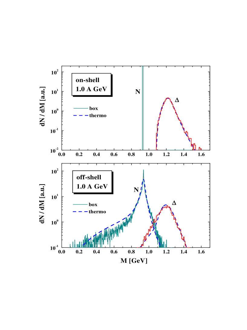
Figure 3: The differential distribution in mass for nucleons and $\Delta$ resonances at equilibrium for an infinite nuclear matter problem at an initial bombarding energy of 1 A GeV at density $\rho=\rho_{0}$. The solid histograms present the results from the transport (box) calculations for the on-shell limit (upper part) and off-shell limit (lower part), respectively. The dashed lines (’thermo’) are obtained from the statistical model at temperature $T=$ 97 MeV employing the spectral functions from the transport approach (see text).

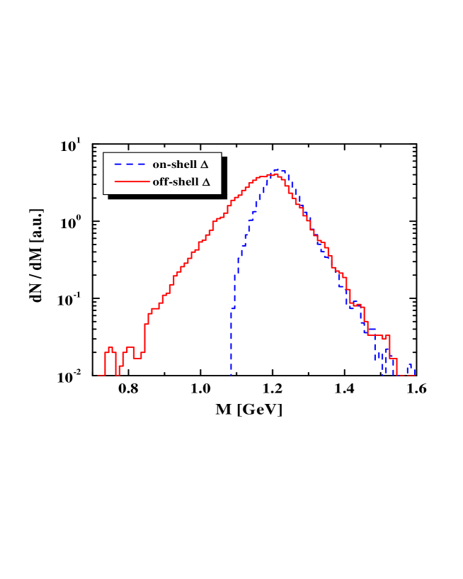
Figure 4: Comparison of the differential distribution in mass for $\Delta$ resonances at equilibrium for the same infinite nuclear matter problem as in Fig. 3. The solid histogram presents the results from the transport calculations for the off-shell limit while the dashed histogram stems from the on-shell calculation.

References

• [1] S. Bass, M. Belkacem, M. Bleicher et al., Prog. Part. Nucl. Phys. 41 (1998) 255.
• [2] W. Cassing and E. L. Bratkovskaya, Phys. Rep. 308 (1999) 65.
• [3] L. P. Kadanoff and G. Baym, Quantum statistical mechanics, Benjamin, New York, 1962.
• [4] P. Danielewicz, Ann. Phys. (N.Y.) 152 (1984) 239; ibid. 305.
• [5] W. Botermans and R. Malfliet, Phys. Rep. 198 (1990) 115.
• [6] R. Malfliet, Prog. Part. Nucl. Phys. 21 (1988) 207.
• [7] P. A. Henning, Nucl. Phys. A 582 (1995) 633; Phys. Rep. 253 (1995) 235.
• [8] C. Greiner and S. Leupold, Ann. Phys. (N.Y.) 270 (1998) 328.
• [9] S. J. Wang, W. Zuo and W. Cassing, Nucl. Phys. A 573 (1994) 245.
• [10] S. J. Wang and W. Cassing, Ann. Phys. (N.Y.) 159 (1985) 328.
• [11] W. Cassing and S. J. Wang, Z. Phys. A 337 (1990) 1.
• [12] W. Cassing, K. Niita and S. J. Wang, Z. Phys. A 331 (1988) 439.
• [13] R. Malfliet, Nucl. Phys. A 545 (1992) 3.
• [14] R. Malfliet, Phys. Rev. B 57 (1998) R11027.
• [15] W. Cassing and S. Juchem, Nucl. Phys. A 665 (2000) 385.
• [16] W. Cassing and S. Juchem, nucl-th/9910052, Nucl. Phys. A, in print.
• [17] S. Leupold, nucl-th/9909080 Nucl. Phys. A, in print.
• [18] E. L. Bratkovskaya, W. Cassing, C. Greiner et al., nucl-th/0001008.
• [19] M. Belkacem, M. Brandstetter, S.A. Bass et al., Phys. Rev. C 58 (1998) 1727.
• [20] L.V. Bravina, M.I. Gorenstein, M. Belkacem et al., Phys. Lett. B 434 (1998) 379; L.V. Bravina, M. Brandstetter, M.I. Gorenstein et al., J. Phys. G 25 (1999) 351.
• [21] L.V. Bravina, E.E. Zabrodin, M.I. Gorenstein et al., Phys. Rev. C 60 (1999) 024904.
• [22] J. Sollfrank, U. Heinz, H. Sorge, N. Xu, Phys. Rev. C 59 (1999) 1637.
• [23] M. Effenberger, E. L. Bratkovskaya and U. Mosel, Phys. Rev. C 60 (1999) 44614.
• [24] M. Effenberger and U. Mosel, Phys. Rev. C 60 (1999) 51901.
• [25] Yu. B. Ivanov, J. Knoll, and D. N. Voskresensky, nucl-th/9905028.
• [26] W. Ehehalt and W. Cassing, Nucl. Phys. A 602 (1996) 449.
• [27] S. Teis, W. Cassing, M. Effenberger et al., Z. Phys. A356 (1997) 421.
• [28] Gy. Wolf, W. Cassing and U. Mosel, Nucl. Phys. A 552 (1993) 549.
• [29] C. Greiner, K. Wagner and P.G. Reinhard, Phys. Rev. C 49 (1994) 1693.
Refer to caption