A hybrid version of the tilted axis cranking model and its application to ¹²⁸Ba

Abstract

A hybrid version the deformed nuclear potential is suggested, which combines a spherical Woods Saxon potential with a deformed Nilsson potential. It removes the problems of the conventional Nilsson potential in the mass 130 region. Based on the hybrid potential, tilted axis cranking calculations are carried out for the magnetic dipole band in ¹²⁸Ba.

I Introduction

The transitional nuclei in the region $A=130-140$ show regular $\Delta I=1$ regular bands, characterized by large $B(M1)/B(E2)$ ratios, the lack of signature splitting and relatively low dynamical moments of inertia [1]. These bands have an intermediate character. They stand between the collective high-$K$ bands of well deformed nuclei, for which collective rotation is the dominant mechanism of generating the angular momentum  , and the magnetic rotation of near spherical nuclei, for which few high-$j$ particles and holes generate most of the angular momentum  by means of the shears mechanism (see, for example [3, 4]). The question of how changes magnetic into collective rotation has not been studied yet. So far, only the magnetic dipole band in ¹²⁸Ba has been investigated [7] from this point of view. Another intriguing question is the possibility of a chiral character of rotation [8]. Their softness with respect to triaxial deformations makes the nuclei in the $A=130$ region particularly good candidates for identifying this new symmetry type.

The Tilted Axis Cranking (TAC) model [2] has turned out to be an appropriate theoretical tool for the description of the magnetic dipole bands. This model is a natural generalization of the cranking model [6] for situations where the axis of rotation does not coincide with a principal axis of the density distribution of the rotating nucleus, and thus the signature is not a good quantum number. Since introduced, TAC has proven to be a reliable approximation for the energies and intraband transitions in both normally and weakly deformed nuclei [4]. However, in the case of the four quasiparticle magnetic dipole band in ¹²⁸Ba, the TAC calculations [7] predicted the wrong parity and a too early termination of the band and provided only fair description of the electro magnetic transition data [9, 10, 11]. ¹²⁸Ba is one of the best studied nuclei in this mass range and the above mentioned $\Delta I=1$ rotational band is a good test case for the TAC model.

The purpose of the present work is to try to identify the origin of the discrepancies and remove them. The version of TAC used in [7] was based on the Nilsson Hamiltonian. The parameters of this well-tried potential were carefully adjusted for various mass regions, where it was successfully used in standard cranking calculations [12] as well as in TAC calculations [4]. However, the $A=130$ region is known to be problematic for the model. In fact no really satisfactory set of Nilsson parameters for this region is available so far[13]. Thus we attribute the discrepancies of the TAC calculations for ¹²⁸Ba [7] with the later measurements [9, 10, 11] to the general problems of the Nilsson potential in this region.

On the other hand, the Woods-Saxon potential works very well around $A=130$ [14]. Encouraged by this, we adapt the Nilsson potential as close as possible to the Woods-Saxon one. We call this the hybrid potential, which is the basis for new TAC calculations for ¹²⁸Ba. Instead of the parameterizing the single particle levels of the spherical modified oscillator in the standard way by means of an $ls$- and an $l^{2}$-term, the hybrid model directly takes the energies of the spherical Woods-Saxon potential. The deformed part of the hybrid potential is an anisotropic harmonic oscillator. This compromise keeps the simplicity of the Nilsson potential, because coupling between the oscillator shell can be approximately taken into account by means of stretched coordinates [12], and it amounts to a minor modification of the existing TAC code. On the other hand, it has turned out to be a quite good approximation of the realistic flat bottom potential as long as the deformation is moderate. The hybrid was used to calculate the triaxial shapes of liquid sodium clusters [15]. The results agree very well with later calculations using the correct radial profile of the deformed part of the potential[16].

II TAC implementation

The TAC model is discussed in more detail in [2, 3, 4, 5]. The brief presentation in this paper focuses at the suggested improvement of this approach. The starting point is the mean field Routhian

$$h^{\prime}=h_{sph}+V_{def}(\varepsilon_{2},\gamma,\varepsilon_{4})\\ -\Delta\left(P+P^{+}\right)-\lambda N-\omega\left(\sin\vartheta\,j_{1}+\cos\vartheta\,j_{3}\right)$$ (1)

where $h_{sph}$ denotes the spherical part including the spin-orbit term and $V_{def}(\varepsilon_{2},\gamma,\varepsilon_{4})$ the deformed part of the Nilsson single-particle Hamiltonian. (see, e.g. [12]). The pairing field in eq.(1) is determined by the gap parameter $\Delta$ and the monopole pairing operator $P=\sum_{k}c_{k}c_{\overline{k}}$ while the chemical potential $\lambda N$ is needed to satisfy on average the particle number conservation. The two-dimensional cranking term $\omega\left(\sin\vartheta\,j_{1}+\cos\vartheta\,j_{3}\right)$ is the new element of the TAC, as compared to the standard cranking model, which is recovered for $\vartheta$ = 0 or 90^∘. The angle $\vartheta$ fixes the tilt of the cranking axis with respect to the intrinsic 3-axis within the principal (1-3) plane of the deformed potential. By diagonalization in stretched coordinates, neglecting $\Delta N=2$ shell mixing, this TAC Routhian yields quasi-particle energies and quasi-particle states, from which the many-body configuration $|\,\omega,\varepsilon_{2},\gamma,\varepsilon_{4},\vartheta>$ of interest is constructed.

The mean field is found for a given frequency $\omega$ and fixed configuration by minimizing the total Routhian

$$E^{\prime}(\omega,\varepsilon_{2},\gamma,\varepsilon_{4},\vartheta)=<\omega,\varepsilon_{2},\gamma,\varepsilon_{4},\vartheta\,|\,h^{\prime}\,|\,\omega,\varepsilon_{2},\gamma,\varepsilon_{4},\vartheta>$$ (2)

with respect to the deformation parameters $(\varepsilon_{2},\gamma,\varepsilon_{4})$ and the tilt angle $\vartheta$. The value of $\Delta$ is kept fixed at two values: 80% of the experimental odd-even mass difference and zero. At the equilibrium angle $\vartheta=\vartheta_{\circ}$ (minimum) the cranking axis is parallel to the direction of the angular momentum vector $\vec{J}=(<j_{1}>,<j_{3}>)$. After the minimum is found the various electro magnetic observables of interest are obtained by means of the following semiclassical expressions [3, 5]

$$<I-2I-2|{\cal M}_{-2}(E2)|II>=<{\cal M}_{-2}(E2)>=$$ (3)

$$=\sqrt{{5\over 4\pi}}\left(\frac{eZ}{A}\right)\left[\sqrt{3\over 8}<Q^{\prime}_{0}>(\sin\,\vartheta)^{2}+{1\over 4}<Q^{\prime}_{2}+Q^{\prime}_{-2}>\left(1+(\cos\vartheta)^{2}\right)\right],$$ (4)

$$<I-1I-1|{\cal M}_{-1}(E2)|II>=<{\cal M}_{-1}(E2)>=$$ (5)

$$=\sqrt{{5\over 4\pi}}\left(\frac{eZ}{A}\right)\left[\sin\,\vartheta\cos\vartheta(\sqrt{3\over 2}<Q^{\prime}_{0}>-{1\over 2}<Q^{\prime}_{2}+Q^{\prime}_{-2}>)\right].$$ (6)

$$<I-1I-1|{\cal M}_{-1}(M1)|II>=<{\cal M}_{-1}(M1)>=$$ (7)

$$=\sqrt{\frac{3}{8\pi}}\left[\mu_{3}\sin\,\vartheta-\mu_{1}\cos\,\vartheta\right],$$ (8)

where $<{\cal M}_{\nu}>$ is the expectation value of the transition operator with the TAC configuration $|>$, the components of which refer to the lab system. The intrinsic quadrupole moments $Q^{\prime}_{\mu}$ are calculated with respect to the principle axes (1, 2, 3). The same holds for the magnetic moments

$$\mu_{1}=\mu_{N}(J_{1,p}+(\eta 5.58-1)\,S_{1,p}-\eta 3.82\,S_{1,n}),~{}~{}\mu_{3}=\mu_{N}(J_{3,p}+(\eta 5.58-1)\,S_{3,p}-\eta 3.82\,S_{3,n}),$$ (9)

where the free nucleonic magnetic moments are attenuated by a factor of $\eta=0.7$. The reduced transition probabilities are

$$B(M1,\Delta I = 1)=<{\cal M}_{-1}(M1)>^{2}$$

$$B(E2,\Delta I = 2)=<{\cal M}_{-2}(E2)>^{2}$$

The mixing ratio is

$$\delta=\frac{<{\cal M}_{-1}(E2)>}{<{\cal M}_{-1}(M1)>}.$$ (10)

We apply the Strutinsky renormalization procedure to calculate the total Routhian

$$E^{\prime}(\omega)=E_{LD}(\omega=0)-E_{smooth}+<\omega|\,h^{\prime\,}|\omega>,$$ (11)

where $E_{LD}=E_{LD}(\varepsilon_{2},\gamma,\varepsilon_{4},\varepsilon_{4})$ means the liquid drop energy and $E_{smooth}$ is the the smooth part of the mean-field energy calculated from the single-particle energies at $\omega=0$. This version of the TAC has turned out to be quite successful for well deformed nuclei (see [3, 4, 5] and references therein).

The new element of the present paper consists in the hybrid potential, which approximates the well-established deformed Woods-Saxon potential, yet preserving the existing convenient TAC environment. For this purpose the spherical part $h_{sph}$ in Eq.(1) is replaced the spherical Woods-Saxon Hamiltonian for the nucleus of interest. In the present work the universal Woods-Saxon parameters are used (see e.g. [17]).

Technically, the replacement is rather simple, because the existing TAC code uses states of good $l,j,m$ as a basis. The spherical Nilsson energies $e^{(nil)}_{N,l,j}$ are replaced by the spherical Woods - Saxon energies $e^{(ws)}_{N,l,j}$. It turns out to be unproblematic to associate the quantum numbers of the two different potentials. For a given combination $l,j$ the third quantum number $N$ is found by counting from the state with the lowest energy. The fact that the spherical Woods-Saxon code uses a harmonic oscillator basis permitted a check of the algorithm. The major component of the Woods-Saxon wavefunction agrees with the state found by our counting algorithm. In the high-lying part of the single-particle spectrum (three shells above the valence shell or higher) there are occasional ambiguities in assigning the states. Small errors of this kind are not expected to have any consequences at moderate or small deformation. The states do not couple strongly to the states near the Fermi surface. They contribute only to the smooth level density used in the Strutinsky renormalization, which will not be affected by small shifts of the levels.

Such a replacement of the spherical single-particle energies is a common practice in large scale shell-model configuration mixing and similar calculations, where they are often used as adjustable parameters [18]. The effect of the replacement is illustrated on Fig.1, which shows the deformation dependence of the proton single-particle levels of ¹²⁸Ba for the Nilsson, the Woods-Saxon and the hybrid Hamiltonians. The close similarity of the levels of the Woods-Saxon and the hybrid models is obvious. The hybrid has a somewhat later and sharper crossing between the positive parity levels, which also show stronger tendency to arrange into pairs of pseudo spin doublets. These treats are inherited from the Nilsson Hamiltonian, which controls the change with deformation. The main difference between the Nilsson Hamiltonian and the other two is the lower energy of the negative parity levels originating from $h_{11/2}$. It seems to be the reason for the discrepancies between the previous TAC predictions and the experiment, as will be demonstrated in the next section.

III The M1 band in ¹²⁸Ba

In the previous TAC calculations for the $\Delta I=1$ band in ¹²⁸Ba [7] the four quasi-particle configurations $[\pi(h_{11/2})^{2}\nu(h_{11/2}(d_{5/2}g_{7/2}))]$ for the negative parity and $[\pi(h_{11/2})^{2}\nu(h_{11/2})^{2}]$ for the positive parity were found to be the lowest ones in energy at the oblate deformation of $\varepsilon=0.26$, $\gamma=60^{o}$. This deformation was determined at $\omega=0.2$ MeV by minimizing the total Routhian calculated from the Quadrupole-Quadrupole interaction. With the present version of TAC we find a significantly smaller prolate equilibrium deformation of $\varepsilon=0.205$ and $\gamma=0^{o}$. The lowest four quasi-particle configuration now turns out to be $[\pi(h_{11/2}(d_{5/2}g_{7/2}))\nu(h_{11/2}(d_{5/2}g_{7/2}))]$. Fig.2 shows the quasi proton and quasi neutron levels for various cranking frequencies at tilt angle $\vartheta=90^{o}$ and for various angles at $\omega=0.2$ MeV. The equilibrium value of $\vartheta$, which minimizes $E^{\prime}$, is found to be $\vartheta_{\circ}=52.5^{o}$ for $\omega=0.2$ MeV.

As seen, the different position of the $h_{11/2}$ orbitals in the hybrid TAC has drastic consequences. The deformation changes from oblate to prolate, resulting in a different configuration of the M1 band. This is not surprising in a region where the energy difference between oblate and prolate shape is small.

The calculations of the $\Delta I=1$ band in the present work are built on this new configuration $[\pi(h_{11/2}(d_{5/2}g_{7/2}))(\nu h_{11/2}(d_{5/2}g_{7/2}))]$, which is the lowest four-quasi particle TAC solution. In agreement with the experiment, it has positive parity. The excitation of four quasi-particles significantly reduces the pairing gaps. In order to better grasp the influence of this blocking on characteristics of the band, we did two calculations: one with $\Delta_{\nu}=0.88$ MeV and $\Delta_{\pi}=1.04$ MeV corresponding to 80% of the experimental even odd mass difference and one with zero pairing.

Electro magnetic transition properties present a stringent test of the nuclear models. The experimental information about lifetimes and mixing ratios of the magnetic dipole band was accumulated in several experiments [9, 10, 11]. Fig.3 compares the experimental $B(M1)$ and $B(E2)$ values and mixing ratios with the results of TAC model obtained for the configuration $[\pi(h_{11/2}(d_{5/2}g_{7/2}))\nu(h_{11/2}(d_{5/2}g_{7/2}))]$. All electro-magnetic characteristics of the band are well reproduced by both the paired and unpaired calculations. Curiously, the quenching of pairing influences to some extent the $B(M1)$ values but leaves almost unchanged the B(E2) values up to spin 18$\hbar$. The TAC calculation seems to slightly overestimate the deformation.

In contrast with the previous TAC calculation, it is possible to follow the band all the way up to spin 26$\hbar$. Fig.4 shows the measured and the calculated function $J(\omega)$ of the spin on the angular frequency. It is more sensitive to the changes of the pair correlations. While the unpaired calculation gives a nearly linear function with the moment of inertia ${\cal J}^{(2)}=dJ/d\omega$ close to the measured one, the paired calculation exhibits a substantially lower moment of inertia for low rotational frequencies and an upbend at higher ones. The experiment is in between. This seems to indicate that the pair field is weak in this nucleus and a more refined treatment of pairing is needed. It is noted that in the calculations the band extends down to $\omega=0.1\,MeV$ and $J=11\hbar$. In experiment there is an irregularity around $I=12,13\hbar$. It may be caused by mixing of the $13^{+}$ state with the another $13^{+}$ state, which lies nearby in energy ($\Delta E=0.045\,MeV$) and into which the $14^{+}$ also decays[11] .

In [9, 10, 11], the $\Delta I=1$ band was analyzed in terms of a pure high-K band using the familiar expressions for the $B(M1)$ and $B(E2)$ values for the axial symmetric rotor [19]. Adjusting three free parameters, the K-value, the intrinsic quadrupole moment $Q_{\circ}$, and the gyromagnetic factor $|g_{K}-g_{R}|$, a good fit of the electro magnetic decay data was obtained. The quality is practically the same as in our calculation without parameters in Fig.4. The TAC calculation contains much more physical information as e.g. the specific configuration on which the band is built and the band energies. The knowledge of the intrinsic state can be used to derive further structure information, e. g. the geometrical coupling scheme shown in Fig.5, which enables one to see how the total spin is formed from the quasiparticle orbitals and how it changes with the rotational frequency. Apparently, most of the angular momentum gain along the band is of collective nature, however the high-j quasiparticles from proton and neutron $(d_{5/2}g_{7/2})$ and $h_{11/2}$ orbitals do also substantially contribute by means of the shears mechanism. With increasing frequency, the 3-component of the spin vector $\vec{J}$ stays practically at $<J_{3}>\approx$ 9$\hbar$. However, this does not mean that the corresponding TAC configuration behaves like a structureless the high-K rotor. Fig.6 shows that the calculated dependence $\vartheta(\omega)$ of the tilt angle on the rotational frequency by no means follows curve expected for the strong coupling limit. Thus, the present case lies in between a good shears band and a good high-K band. The $\Delta I=1$ band in ¹²⁸Ba is an example for a rotational band of intermediate nature.

IV Summary

The strength of the TAC model is that it can predict the appearance of $\Delta I=1$ rotational bands and is able to describe microscopically their electro magnetic decay properties. This is achieved by taking into consideration the orientation of the rotational axis with respect to the deformed potential, which is fixed along a principal axis in the conventional cranking model. The intrinsic TAC configuration of a rotational band is found by searching for a local minimum on the multi-parameter surface of the total Routhian. Therefore, it is crucial to calculate these surfaces as reliable as possible. In the present work the Strutinsky renormalization and a hybrid single-particle potential were implemented in order to improve the total Routhian. The hybrid potential combines the spherical Woods-Saxon single-particle energies with the deformed part of the Nilsson potential. For moderately deformed nuclei it gives deformed single-particle levels that are quite close to the deformed Woods-Saxon levels.

We applied the hybrid TAC to the previously investigated four quasiparticle magnetic dipole band in ¹²⁸Ba. The lowest equilibrium configuration is found to be $[\pi(h_{11/2}(d_{5/2}g_{7/2}))\nu(h_{11/2}(d_{5/2}g_{7/2}))]$. It has positive parity and a prolate axial deformation of $\varepsilon_{2}=0.20$. The microscopic TAC calculations describes rather well the experimental energies, $B(M1)$ and $B(E2)$ values, as well as the branching and mixing ratios. The dipole band in ¹²⁸Ba has an intermediate structure. A comparable amount of angular momentum is generated by the shears mechanism, active for the $h_{11/2}$ and $(d_{5/2}g_{7/2})$ quasiparticles, and by collective rotation. It is an example for the transition from collective to magnetic rotation.

The hybrid potential turned out to be crucial for the good agreement between the calculation and the data. It substantially improves the Nilsson potential, which has problems in the region around mass 130. It seems to be a promising starting point for studying the intriguing interplay between triaxial deformation and the orientation of the rotational axis.

V Acknowledgments

V.D. wishes to thank the Foundation ”Bulgarian Science and Culture” for its support. We should like to thank Prof. P. von Brentano and Dr. I. Wiedenhöver, who kept us up with the data. The work was partially carried out under the Grant DE-FG02-95ER40934.

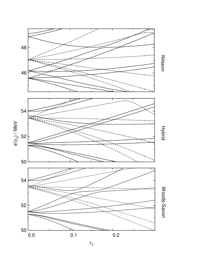
FIG. 1.: Proton single-particle levels as function of deformation for the Woods-Saxon (bottom), hybrid (middle) and Nilsson (top) model, respectively. Full lines present positive parity states, broken lines - negative parity states. The Fermi energy lies at about 51.3 MeV for the Woods-Saxon and the hybrid models and at 45.6 MeV for the Nilsson model.

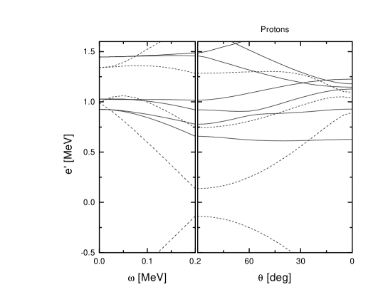
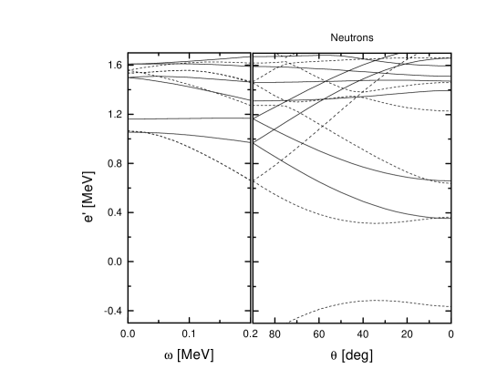
FIG. 2.: Proton (a) and neutron (b) quasi-particle levels as function of rotational frequency $\hbar\omega$ and tilt angle $\vartheta$. Full lines correspond to positive parity, broken lines - to negative parity states. In both cases the lowest two quasi-particle configurations involve one predominantly $(d_{5/2}g_{7/2})$ and one predominantly $h_{11/2}$ state. The deformation parameters are $\varepsilon_{2}=0.205,\varepsilon_{4}=-0.01,\gamma=0^{o}$, which are the equilibrium values at $\omega=0.2~{}MeV$.

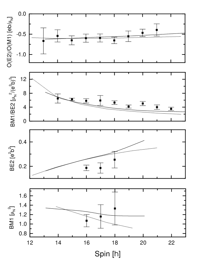
FIG. 3.: Electromagnetic observables as obtained by paired calculation (full lines), unpaired calculation (dotted lines) and experiment.

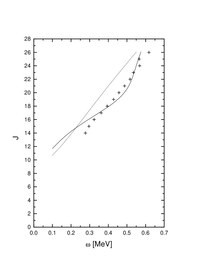
FIG. 4.: Dependence of the angular momentum $J=I$ on the rotational frequency $\hbar\omega$ as obtained by paired calculation (full line), unpaired calculation (dotted line) and experiment (crosses). The experimental frequency is extracted from the measured $\gamma-$energy data using the relations $\hbar\omega(I)=E_{\gamma}=E(I)-E(I-1)$.

FIG. 5.: Spin decomposition in terms of individual quasi-particle contributions for two different rotational frequencies. Quasi-particle configurations are denoted by their predominant components.

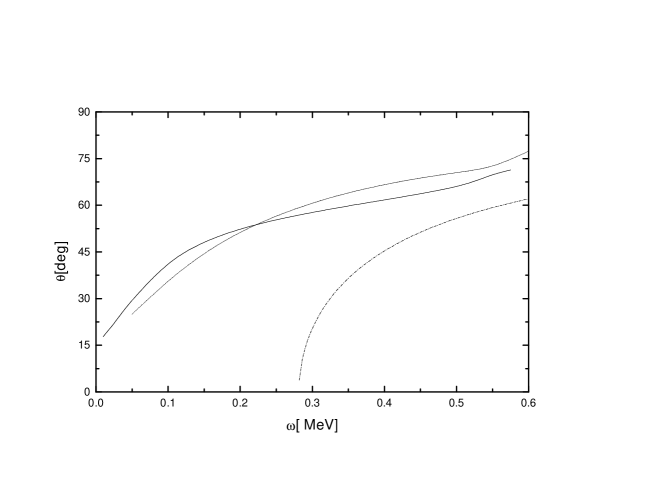
FIG. 6.: Equilibrium tilt angle $\vartheta$ as a function of the rotational frequency $\hbar\omega$. Full line - paired calculation; dotted line - unpaired calculation; broken-dotted line - strong coupling limit result.

REFERENCES

-
[1]
see, for example D. Fossan, J. R. Hughes, Y. Liang,
R. Ma, E. S. Paul, and N. Xu,
Nucl. Phys. A520, 241c - [2] S.Frauendorf, Nucl.Phys. A557 (1993) p.259c
- [3] S. Frauendorf, Z. Phys. A385, 163 (1997)
- [4] S. Frauendorf, Rev. Mod. Phys, submitted
- [5] S. Frauendorf,Nucl. Phys. A, submitted
- [6] P.Ring, P.Schuck; The Nuclear Many Body Problem, Springer NY 1980
-
[7]
F.Dönau, S. Frauendorf, P. von Brentano,
A. Gelberg, and O. Vogel ,
Nucl.Phys A584 (1995) p.241; - [8] S. Frauendorf, and Meng, J., 1997,Nucl. Phys. A 617, 131 (1997)
- [9] O.Vogel, A. Dewald, P. von Brentano, J. Gableske, R. Krücken, N. Nicolay, A. Gelberg, P. Petkov, A. Gizon, J. Gizon, D. Bazacco, C. Rossi Alvarez, S. Lunardi, P. Pavan, D.R. Napoli, S. Frauendorf, and F. Dönau , Phys.Rev. C56 (1997) p.1338
- [10] P. Petkov, J. Gablenske, O. Vogel, A. Dewald, P. von Brentano, R. Krücken, R. Peusquens, N. Nicolay, A. Gizon, J. Gizon, D. Bazacco, C. Rossi-Alvarez, S. Lunardi, P. Pavan, D.R. Napoli, W. Andrejtscheff, R.V. Jolos, Nucl. Phys. A 640 (1998) 293
- [11] I. Wiedenhöver, O. Vogel, H. Klein, A. Dewald, P. von Brentano, J. Gableske, R. Krücken, N. Nicolay, A. Gelberg, P. Petkov, A. Gizon, D. Bazzacco, C. Rossi Alvarez, G. de Angelis, S. Lunardi, P. Pavan, D.R. Napoli, S. Frauendorf, F. Dönau, R.V.F. Janssens,and M. Carpender , Phys.Rev. C58 (1998) p.721
- [12] S.G. Nilsson and I. Ragnarsson, Shapes and Shells in Nuclear Structure, Cambridge University Press, 1995
- [13] R. Bengtsson, private communication
- [14] Wyss, R., Granderath, A., Bengtsson, R., von Brentano, P., Dewald, A., Gelberg, A., Gizon, A., Gizon, J., Harissopulos, S., Johnson, A., Lieberz, W., Nazarewicz, W., Nyberg, J., and K. Schiffer, Nucl. Phys. A 505, 337 (1989)
- [15] S. Reimann, S. Frauendorf, M. Brack,Z. Phys. D 34, 125 (1995)
-
[16]
B. Montag, Th. Hirschmann, J Meyer, P.-G. Reinhard, M. Brack,
Phys. Rev. B 52, 4775 (1995) - [17] S.Cwiok, J. Dudek, W. Nazarevicz, J. Skalski, and T. Werner, Comput. Phys.Commun.. 46 (1987) 379
-
[18]
M.Ted Ressell, Maurice B. Aufderheide, Steward D. Bloom,
Kim Griest, Grant J. Mathews, and David A. Resler Phys.Rev. D48 (1993)
p.5519;
V.I.Dimitrov, J. Engel and S. Pittel, Phys.Rev. D51 (1995) R291 - [19] A. Bohr and B.M. Mottelson, Nuclear Structure Vol. II, W.A. Benjamin, Reading, MA, 1957