Quantum Monte Carlo calculations of six-quark states

Abstract

The variational Monte Carlo method is used to find the ground state of six quarks confined to a cavity of diameter $R_{c}$, interacting via an assumed non-relativistic constituent quark model (CQM) Hamiltonian. We use a flux-tube model augmented with one-gluon and one-pion exchange interactions, which has been successful in describing single hadron spectra. The variational wave function is written as a product of three-quark nucleon states with correlations between quarks in different nucleons. We study the role of quark exchange effects by allowing flux-tube configuration mixing. An accurate six-body variational wave function is obtained. It has only $\sim 13\%$ rms fluctuation in the total energy and yields a standard deviation of $\lesssim.1\%$; small enough to be useful in discerning nuclear interaction effects from the large rest mass of the two nucleons. Results are presented for three values of the cavity diameter, $R_{c}=2$, 4, and 6 fm. They indicate that the flux-tube model Hamiltonian with gluon and pion exchange requires revisions in order to obtain agreement with the energies estimated from realistic two-nucleon interactions. We calculate the two-quark probability distribution functions and show how they may be used to study and adjust the model Hamiltonian.

I Introduction

The constituent quark model (CQM) has been useful to describe the spectroscopy isgur:3q ; robson:3q ; ckp2 and the decay isgur:decay ; stancu ; kumano1 of baryons and mesons. It retains only the constituent quark (CQ) degrees-of-freedom; the effects of all other degrees-of-freedom are subsumed into potentials dependent upon CQ positions, spins, flavors and colors. It assumes that a Hamiltonian describing interacting quarks can provide a useful description of the low-energy properties of hadrons.

It is natural to attempt to extend the CQM to describe the two-baryon states made up of six CQ. The only such bound state known is the deuteron; all other known two-baryon states are unbound. The scattering data provides information on the interaction between baryons which is used to construct realistic models of the two-baryon potential nijmegen ; wiringa:av18 ; rijken .

Many authors isgur:6q ; oka84 ; robson:6q have attempted to calculate properties of two-baryon states, including the interaction between nucleons, using the CQM. In these studies some approximation scheme is used to avoid the calculation of six-body eigenstates of the assumed CQM Hamiltonian. In the past few years there have been significant advances in the variational (VMC) and Green’s function Monte Carlo (GFMC) methods to calculate the eigenstates of up to eight interacting nucleons pudliner1 ; wiringa00 . In these quantum Monte Carlo (QMC) methods a good approximate solution is first obtained by the VMC method from which the exact eigenstate is projected with the GFMC.

In the present work we attempt to find the ground state of two-nucleons confined to a spherical cavity of diameter $R_{c}$ in the center-of-mass frame using the CQM. In the interior of the cavity the six CQ wave function is determined with VMC. Near the edge of the cavity we assume that it factorizes into a two-nucleon wave function required to be zero at the internucleon distance $R_{c}$.

This problem may be easily solved assuming that the ground state can be described as that of two interacting nucleons. The deuteron has total spin-isopin, $S,T=1,0$, and in local, realistic models such as Argonne $v_{18}$ wiringa:av18 , the nuclear interaction in the deuteron is given by a sum of central, tensor, and spin-orbit potentials: $v_{d}^{c}(r)$, $v_{d}^{t}(r)$ and $v_{d}^{\ell s}(r)$. The two-nucleon Schrödinger equation:

$$-\frac{\hbar^{2}}{m_{N}}\frac{d^{2}}{dr^{2}}u(r)+v_{d}^{c}(r)u(r)+\sqrt{8}v_{d}^{t}(r)w(r) = E(R_{c})u(r)$$ (1)

$$-\frac{\hbar^{2}}{m_{N}}\left(\frac{d^{2}}{dr^{2}}-\frac{6}{r^{2}}\right)w(r)+\left(v_{d}^{c}(r)-2v_{d}^{t}(r)-3v_{d}^{\ell s}(r)\right)w(r)$$

$$+\sqrt{8}v_{d}^{t}(r)u(r) = E(R_{c})w(r)$$ (2)

where $m_{N}$ is the average mass of the neutron and proton, and $u(r)$ and $w(r)$, the ${{}^{3}S}_{1}$ and ${{}^{3}D}_{1}$ wave functions, can be easily solved with the boundary conditions $u(R_{c})=w(R_{c})=0$. The results obtained with the $v_{18}$ model are shown in Table 1 for $R_{c}=$ 2, 4, and 6 fm. They presumably have small dependence on the model $NN$ interaction because all models have mostly the one-pion exchange potential (OPEP), $v^{\pi}_{NN}$ at $r>2$ fm in $T=0$ states. Note that $E(R_{c}\to\infty)$ is just the deuteron binding energy of $-2.24$ MeV, for the isoscalar part of Argonne $v_{18}$.

The $E(R_{c})=\langle T_{N}\rangle+\langle v_{NN}\rangle$, has a large cancellation between the nucleon kinetic energy $\langle T_{N}\rangle$ and the negative two-nucleon interaction energy $\langle v_{NN}\rangle$, typical of nuclear systems pudliner1 . In Table 1 we also list the energy,

$$E_{NI}(R_{c})=\frac{\pi^{2}\hbar^{2}}{m_{N}R_{c}^{2}},$$ (3)

of two non-interacting nucleons in a cavity of diameter $R_{c}$ and the total effect $\delta E_{emp}(R_{c})=E(R_{c})-E_{NI}(R_{c})$ of strong interactions, per nucleon. Our long-range aim is to calculate $E(R_{c})$, and thus $\delta E(R_{c})$, with computational errors of $<1$ MeV using CQM, and compare with the $\delta E_{emp}(R_{c})$, calculated from Argonne $v_{18}$ potential, which reproduces the known $NN$ data. These calculations can then be used to refine the CQM Hamiltonian and study the behavior of the wave function in the region where the six CQ are close together, i.e. the region in which the quark distributions of the two-nucleons overlap. Eventually such calculations may be useful to study $\Lambda-N$ and $\Sigma-N$ interactions for which the scattering data is limited.

The first main concern in this approach is that the total energy, $E_{V}$, in the CQM includes the rest mass of the nucleons, and is therefore of order $2m_{N}\sim$ 2000 MeV. In order to calculate this energy with an accuracy of $\sim 1$ MeV the variance of the local energy,

$$E_{V}(\mathbf{R})=\frac{\Psi_{V}^{\dagger}(\mathbf{R})\hat{H}\Psi_{V}(\mathbf{R})}{\Psi_{V}^{\dagger}(\mathbf{R})\Psi_{V}(\mathbf{R})},$$ (4)

where $\mathbf{R}=\{\mathbf{r}_{1},\mathbf{r}_{2},\dots,\mathbf{r}_{6}\}$ is the six CQ configuration and $\Psi_{V}(\mathbf{R})$ is the variational wave function, must be sufficiently small so that the Monte Carlo statistical error is of $\lesssim 1$ MeV. A major focus of this work is on developing six CQ wave functions with small variance of the local energy. The exact eigenstate satisfies $\hat{H}\Psi_{0}(\mathbf{R})=E_{0}\Psi_{0}(\mathbf{R})$ at all $\mathbf{R}$, and hence has zero variance. The Monte Carlo statistical errors in GFMC calculations are also determined by the variance of $E_{V}(\mathbf{R})$, thus it is necessary to obtain variational wave functions with small variance before proceeding to GFMC.

The second main concern is the choice of the CQM Hamiltonian. Our $\hat{H}$ is basically a generalization of the Y-junction flux-tube (FT) model ckp2 ; ckp1 . The model Hamiltonian in Ref.ckp2 (herein referred to as CKP) contains relativistic CQ kinetic energies, Y-junction FT confinement potential and one-gluon exchange Coulomb, $\mbox{\boldmath{$\sigma$}}_{i}\cdot\mbox{\boldmath{$\sigma$}}_{j}$, tensor and spin-orbit interactions. It is not suitable to study six-quark systems for at least two reasons.

Any model Hamiltonian used for six light quarks must be able to describe two free nucleons. In order to do that it must give $E(\mathbf{p})=m_{N}+p^{2}/(2m_{N})$ for the energy of a nucleon with momentum $p\ll m_{N}$. This requirement is easily acheived in non-relativistic Hamiltonians by choosing the mass $m_{Q}$ of the CQ as $m_{N}/3$. In the Hamiltonians containing relativistic kinetic energies it is necessary to include boost corrections carlson:rel ; forest:rel1 to all interactions to satisfy this requirement. These are absent in the CKP Hamiltonian. In order to avoid them we begin with the non-relativistic model. However, the CQ momenta are often greater than $m_{N}/3$, and it will be necessary to work with the relativistic Hamiltonian to obtain more reliable results. The present calculation is just the first step.

Second, it is well known that nucleons a few fermi apart interact via the OPEP. It has been shown that the tensor force in the OPEP largely determines the toroidal structure of the deuteron donuts . The model Hamiltonian of CKP does not contain pion-exchange interactions. Within that approach, the emission and absorption of pions by nucleons may be attributed to breaking of flux-tubes kumano2 , an effect absent in our present work. The simplest way to include such processes in our CQM, which we adopt, is by coupling pion fields to the CQ.

The advantages of replacing the one-gluon exchange (OGE) interaction in CQM by OPE, as well as the problems associated with this have been recently discussed by Glozman and Riska riska96 ; glozman99 and by Isgur isgur99 . In our model we include both OGE and OPE interactions between the CQ. They respectively respresent the effect of virtual gluons and color-singlet $q\bar{q}$ pairs missing in the CQM Hamiltonian, and both should be included. A more realistic CQM Hamiltonian may contain additional meson-exchange terms, as discussed in Sec.IV.

The details of the CQM Hamiltonian used in this work are given in Sec.II, and the variational wave function and VMC calculations are described in Sec.III. The results, indicating the limitations of the present Hamiltonian, are presented and discussed in the last section, Sec.IV. Continuing research and conclusions are given in the last Sec.V.

II Flux-tube constituent quark model Hamiltonian

II.1 Single nucleon Hamiltonian

The Hamiltonian for the single nucleon is written as a sum of kinetic energy and two and three-body potential operators,

$$\hat{H}_{N}=\sum_{i=1}^{3}\left(m_{Q}+{\hat{\mathbf{p}}_{i}^{2}\over 2m_{Q}}\right)+\sum_{i<j=1}^{3}\hat{v}_{ij}+V_{3}-V_{0}.$$ (5)

The two-body term, $\hat{v}_{ij}$ is summed over pairs $(ij)$, and $V_{3}$ is a three-body interaction. These potentials are due to FT confinement, and perturbative OGE and OPE between constituent quarks. The $V_{0}$ includes all constants in the long range confining interaction and is taken as a parameter to fit the mass of the nucleon. In the case of the single nucleon in its rest frame, the constituent quark mass, $m_{Q}$, is simply a parameter which may be arbitrarily chosen to obtain agreement with experimental data. However, in the present non-relativistic $6Q$ Hamiltonian the constituent quark mass must be one-third of the nucleon mass for the Hamiltonian to reduce to that of two free nucleons when two three-quark clusters are far apart. For this reason we use $m_{Q}=m_{N}/3$ in this work.

We use the $SU(3)$ FT model of long-range confinement ckp1 . The energy of the flux tubes connecting the three quarks is given by,

$$V^{C}(\mathbf{r}_{1},\mathbf{r}_{2},\mathbf{r}_{3})=\sqrt{\sigma}\sum_{i=1}^{3}r_{iY},$$ (6)

where $r_{iY}$ is the length of the vector $\mathbf{r}_{iY}=\mathbf{r}_{i}-\mathbf{r}_{Y}$, $\mathbf{r}_{Y}$ is the location of the “Y-junction” of the three flux-tubes determined by the minimization of $V^{C}$ with respect to $\mathbf{r}_{Y}$. The renormalized string tension, $\sqrt{\sigma}$, is fixed from the observed single-hadron Regge trajectories. Following Johnson and Thornjohnson:regge we assume,

$$E_{J}^{2}=2\pi\sqrt{\sigma}J\ ,$$ (7)

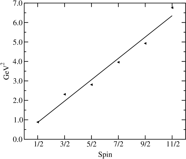
Figure 1: Nucleon mass squared versus $J$ in GeV². The slope is reproduced with string tension $\sqrt{\sigma}=0.88$ GeV.

where $E_{J}$ is the mass of the state with angular momentum $J$. The fit obtained for the nucleon trajectory is shown in Fig.(1), The slope gives $\sqrt{\sigma}=0.88$ GeV/fm; a similar analysis of $\Delta$ resonances produces essentially the same result. This value of $\sqrt{\sigma}$, used here is smaller than the 1 GeV/fm used by CKP.

Considered as quantum strings, the flux-tubes undergo zero-point oscillations which give rise to a constant term, which is included in the $V_{0}$, and terms which depend inversely on the lengths $r_{iY}$ isgur:ftm . The latter are approximately merged into the color Coulomb potential.

We may break-up $V^{C}$ into two- and three-body terms,

$$V^{C}(\mathbf{r}_{1},\mathbf{r}_{2},\mathbf{r}_{3})={1\over 2}\sqrt{\sigma}\sum_{i<j=1}^{3}r_{ij}+V_{3}\ ,$$ (8)

by defining the three-body potential:

$$V_{3}=\sqrt{\sigma}\left(\sum_{i=1}^{3}r_{iY}-{1\over 2}\sum_{i<j=1}^{3}r_{ij}\right).$$ (9)

This break-up is useful because the ratio of the three-body to the two-body term is $\leq 0.154$ for all configurations, saturating when the quarks lie on the vertices of an equilateral triangle. The $V_{3}$ term is zero when the quarks are in a line, and approaches zero when one of the quarks is far from the other two.

The FT confinement model is suggested by numerical studies of lattice QCD which show the interaction between static quarks to be linear in the quark separation at large distances and independent of their spin and isospin stack . The mechanism which gives rise to a linear confining interaction was originally studied by Wilson wilson and others using path-integral methods. Both lattice QCD and path-integral methods indicate that at strong-coupling or, equivalently at length scales of order of the characteristic length scale of QCD, believed to be $\sim 0.5$ fm marciano , the gluonic flux coalesces into tube or string-like configurations due to an attractive self-interaction of the gluons.

We also make the assumption that the flux-tubes move adiabatically, the quarks remaining on their lowest-energy surface. The quarks therefore determine the locations of the flux-tubes and neither the flux nor the Y-junction are free dynamical variables. This seems to be a rather good approximation since, as shown in Ref.page , the lowest lying hybrid states, which take into account dynamics of the flux-tubes, appear to be $\sim 1$ GeV above the nucleon. FT topologies which have more than one Y-junction or loops of flux correspond to higher energy surfaces isgur:ftm and are ignored.

As the distance between sources gets very large flux-tubes may break with concomitant quark-antiquark pair creation. This process has been used to describe the two-pion decays of mesons kumano1 as well as decays of baryons kumano2 . The FT connected to a given quark $i$ may break and the broken piece can reattach to the tube of a different quark $j$. The effects of such interactions between quarks $i$ and $j$ are to be included in the meson exchange terms in CQM Hamiltonian. Of these we consider only the OPE in this work. The virtual $q\bar{q}$ creation also renormalizes the string tension to its physical value isgur:ftm .

The total two-quark potential $\hat{v}_{ij}$ is given by the sum of confinement, perturbative OGE and OPE potentials denoted by $\hat{v}^{g}_{ij}$ and $\hat{v}^{\pi}_{ij}$:

$$\hat{v}_{ij}={1\over 2}\sqrt{\sigma}\ r_{ij}+\hat{v}^{g}_{ij}+\hat{v}^{\pi}_{ij}.$$ (10)

The OGE potential was first used in a CQM by DeRújula, Georgi, and Glashow DGG who showed that the splitting within single-hadron multiplets are qualitatively consistent with those expected from OGE interaction. The OGE potential is the QCD analogue of the Fermi-Breit interaction in QED.

For point particles the OGE spin interactions are singular in nonrelativistic theory. Taking into account the finite size of CQ, we may regulate the potentials in order to obtain solutions of the Schrödinger equation. We use “monopole” form factors at each vertex

$$F(\mathbf{q}^{2})={\Lambda^{2}\over\Lambda^{2}+\mathbf{q}^{2}}$$ (11)

where $\mathbf{q}$ is the three-momentum transfer and $\Lambda$ is the momentum space cutoff, which we take to be 5 fm^-1. The color-charge density of quarks is Yukawa-like with this form factor. The $\hat{v}^{g}_{ij}$ is approximated by:

$$\hat{v}^{g}_{ij}=\sum_{p=c,\sigma,t,\ell s}v^{g}_{p}(r_{ij})O^{p}_{ij}\mathbf{\mathsf{T}}_{i}\cdot\mathbf{\mathsf{T}}_{j}$$ (12)

where the $p=c$ term is the color-Coulomb interaction with $O^{c}_{ij}=\openone$; $p=\sigma$ term denotes the color-magnetic contact interaction with $O^{\sigma}_{ij}=\mbox{\boldmath{$\sigma$}}_{i}\cdot\mbox{\boldmath{$\sigma$}}_{j}$; $t$ is for the tensor interaction, $O^{t}_{ij}=S_{ij}=3\mbox{\boldmath{$\sigma$}}_{i}\cdot\mathbf{\hat{r}}_{ij}\mbox{\boldmath{$\sigma$}}_{j}\cdot\mathbf{\hat{r}}_{ij}-\mbox{\boldmath{$\sigma$}}_{i}\cdot\mbox{\boldmath{$\sigma$}}_{j}$; and $\ell s$ is the spin-orbit contribution, $O^{\ell s}_{ij}=\mathbf{L}_{ij}\cdot\mathbf{S}_{ij}$. The operator $\mathbf{\mathsf{T}}_{i}\cdot\mathbf{\mathsf{T}}_{j}$ is the quadratic Casimir of $SU(3)$ acting on color indices of the quarks. The color wave function of three quark states is antisymmetric. It is an eigenstate of $\mathbf{\mathsf{T}}_{i}\cdot\mathbf{\mathsf{T}}_{j}$ with eigenvalue $-2/3$. The specific forms of the monopole regulated potential functions:

$$v^{g}_{c}(r) ={\alpha_{s}\over r}\left[1-\left({\Lambda r\over 2}+1\right)e^{-\Lambda r}\right]$$ (13)

$$v^{g}_{\sigma}(r) =-{\alpha_{s}\over 12m_{Q}^{2}}\Lambda^{3}e^{-\Lambda r}$$ (14)

$$v^{g}_{t}(r) =-{\alpha_{s}\over 4m_{Q}^{2}}\left[{1\over r^{3}}-{\Lambda^{3}\over 3}\left(T_{\Lambda}(r)+{1\over 2}\left(\Lambda r+1\right)Y_{\Lambda}(r)\right)\right]$$ (15)

$$v^{g}_{\ell s}(r) =-{3\alpha_{s}\over 2m_{Q}^{2}}\left[{1\over r^{3}}-{\Lambda^{2}\over r}\left({1\over\Lambda r}+1+\Lambda r\right)Y_{\Lambda}(r)\right]$$ (16)

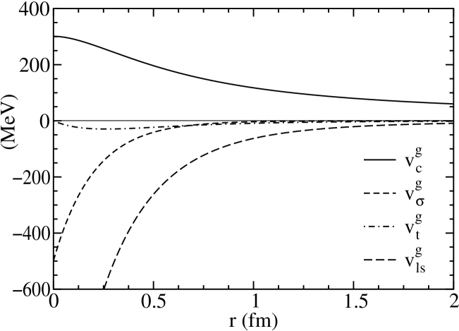
Figure 2: Regulated OGE potential in MeV.

are plotted in Fig.(2). The functions $Y_{\Lambda}$ and $T_{\Lambda}$ are the Yukawa and tensor functions,

$$Y_{\Lambda}(r) = \frac{e^{-\Lambda r}}{\Lambda r}$$ (17)

$$T_{\Lambda}(r) = \left(1+\frac{3}{\Lambda r}+\frac{3}{\Lambda^{2}r^{2}}\right)Y_{\Lambda}(r)$$ (18)

The strength of the OGE potentials is given by the perturbative strong coupling constant, $\alpha_{s}$. We fix the value of $\alpha_{s}=0.61$, consistent with values in earlier works, to reproduce the $N$–$\Delta$ splitting.

The OGE tensor and spin-orbit terms are not as well-established as the color-Coulomb and the short-ranged spin-spin terms; the latter gives a large contribution to the splitting of the pseudoscalar mesons, $\pi-\rho$, and of the S-wave baryons, $N-\Delta$, while the Coulomb term is seen in lattice QCD treatments of the static $QQ$ potential stack .

There is much discussion in the literature concerning the apparent lack of the spin-orbit term ckp2 ; isgur:qm ; myrher in nucleon spectra. Many workers simply discard the longe-range, spin-dependent parts of OGE–the tensor and spin-orbit forces–arguing that those terms may be significantly modified by FT formation and are not well-supported by experimental data. Isgur isgur:3q has argued that the OGE spin-orbit term exists, but it primarily cancels the neglected spin-orbit interaction due to the Thomas precession in the confining FT potential. Oka and Yazaki oka84 have shown that the tensor part of $\hat{v}^{g}_{ij}$ also gives a small contribution to the baryon-baryon interactions. Neither the spin-orbit nor tensor parts of $\hat{v}^{g}_{ij}$ seem to be important in determining the $NN$ interaction in the state with deuteron quantum numbers.

The OPE interaction has the form,

$$\hat{v}^{\pi}_{ij}=\left[v^{\pi,SR}_{\sigma\tau}(r_{ij})+v^{\pi,LR}_{\sigma\tau}(r_{ij})\right]\mbox{\boldmath{$\sigma$}}_{i}\cdot\mbox{\boldmath{$\sigma$}}_{j}\mbox{\boldmath{$\tau$}}_{i}\cdot\mbox{\boldmath{$\tau$}}_{j}+v^{\pi}_{t\tau}(r_{ij})S_{ij}\mbox{\boldmath{$\tau$}}_{i}\cdot\mbox{\boldmath{$\tau$}}_{j}.$$ (19)

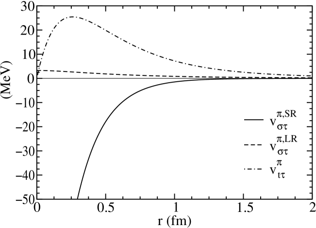
Figure 3: Regulated OPE potential in MeV.

For point particles, $v^{\pi,SR}_{\sigma\tau}(r_{ij})$ is the $\delta$-function part, while $v^{\pi,LR}_{\sigma\tau}(r_{ij})$ is the Yukawa function part of the $\mbox{\boldmath{$\sigma$}}_{i}\cdot\mbox{\boldmath{$\sigma$}}_{j}\mbox{\boldmath{$\tau$}}_{i}\cdot\mbox{\boldmath{$\tau$}}_{j}$ interaction. The quark form factors modify the radial functions, plotted in Fig.(3), as follows:

$$v^{\pi,SR}_{\sigma\tau}(r) = {f_{\pi QQ}^{2}\over 4\pi}{1\over 3}\mu\left[-{1\over 2}{\Lambda^{3}\over\mu^{3}}\left(1-\frac{\mu^{2}}{\Lambda^{2}}\right)^{2}e^{-\Lambda r}\right]$$ (20)

$$v^{\pi,LR}_{\sigma\tau}(r) = {f_{\pi QQ}^{2}\over 4\pi}{1\over 3}\mu\left[Y_{\mu}(r)-{\Lambda\over\mu}Y_{\Lambda}(r)-{1\over 2}\left({\Lambda\over\mu}-{\mu\over\Lambda}\right)e^{-\Lambda r}\right]$$ (21)

$$v^{\pi}_{t\tau}(r) = {f_{\pi QQ}^{2}\over 4\pi}{1\over 3}\mu$$ (22)

$$\times\left[T_{\mu}(r)-{\Lambda^{3}\over\mu^{3}}T_{\Lambda}(r)-{1\over 2}{\Lambda\over\mu}\left({\Lambda^{2}\over\mu^{2}}-1\right)\left(\Lambda r+1\right)Y_{\Lambda}(r)\right].$$

Here $\mu=138$ MeV, the average mass of the three charge states of the pion, and $Y_{\mu}$ and $T_{\mu}$ are as given in Eqs.(17,18) with $\Lambda\to\mu$. Note that $v^{\pi,SR}_{\sigma\tau}$ and $v^{\pi,LR}_{\sigma\tau}$ have equal and opposite volume integrals.

At large distances the sum of OPE interactions between the nine pairs of quarks in different nucleons must be equivalent to the $NN$ OPEP tail. Thus we fix the coupling constant, $f_{\pi QQ}^{2}/4\pi$, by considering a configuration of quarks representing two well separated nucleons. In this limit the ratio of the sum of OPE interactions between the quarks of different nucleons and the $v^{\pi}_{NN}$ contains the $SU(2)_{spin}\otimes SU(2)_{flavor}$ factor of $9/25$. Therefore:

$$f_{\pi QQ}={3\over 5}f_{\pi NN},$$ (23)

where the pion-nucleon coupling constant $f_{\pi NN}$ is known from $NN$ scattering experiments to be $f_{\pi NN}^{2}/4\pi=0.075$stoks . Since the quoted value of the $\pi NN$ coupling constant is extrapolated to pion-pole, the monopole form factor:

$$F(\mathbf{q}^{2})={\Lambda^{2}-\mu^{2}\over\Lambda^{2}+\mathbf{q}^{2}},$$ (24)

containing the pion mass $\mu$ is used to calculate the $\hat{v}^{\pi}$. We assume that the cutoff parameter $\Lambda$ is the same for OGE and OPE interactions between quarks, though they could be different.

Presumably we are justified in retaining the long-range parts, $v^{\pi,LR}_{\sigma\tau}(r)$ and $v^{\pi}_{t\tau}(r)$, of OPEP. The short-range $v^{\pi,SR}_{\sigma\tau}(r)$, term however, is the smeared delta-function contact potential whose validity is questionable. Within the meson exchange picture one expects an infinite number of $q\bar{q}$ states to contribute at short distances. The contribution of higher mass meson states can modify the strength of the contact term.

The single $N$ and $\Delta$ properties calculated with this Hamiltonian are listed in the rightmost columns of Table 2. We note several features of these results. The kinetic energy of the quarks in the $\Delta$–resonance is significantly smaller than that in the nucleon, thus the $N-\Delta$ mass difference cannot be calculated perturbatively as was noted by CKP.

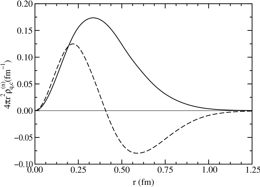
Figure 4: Neutron radial quark density, $4\pi r^{2}\rho^{(n)}_{q}$ (solid line) and radial charge density, $4\pi r^{2}\rho^{(n)}_{c}$ (dashed line) scaled by 10.

The $v^{\pi,SR}_{\sigma\tau}$ term makes a significant contribution to the nucleon energy and the $N-\Delta$ mass difference. The nucleon is composed primarily of $T=0,S=0$ and $T=1,S=1$ pairs, with nearly half the pairs in each channel. The value of $\mbox{\boldmath{$\sigma$}}_{i}\cdot\mbox{\boldmath{$\sigma$}}_{j}\mbox{\boldmath{$\tau$}}_{i}\cdot\mbox{\boldmath{$\tau$}}_{j}$ in these pairs are +9 and +1, respectively. The $\Delta$ however has $T=1,S=1$ pairs almost exclusively. This results in a strong attractive short-range pion interaction in the nucleon relative to the $\Delta$ and causes the $d$ $(u)$ quark in the proton (neutron) to have a smaller rms radius than the average. This effect may be seen in the neutron charge density, $\rho^{(n)}_{c}$, plotted along with the quark density $\rho^{(n)}_{q}$ in Fig.(4).

The other short-ranged interaction is the $v^{g}_{\sigma}$ term in $\hat{v}^{g}_{ij}$. Its contributions to the energy of the nucleon and the $N-\Delta$ mass difference are of the same order as those of $v^{\pi,SR}_{ij}$. In fact, one can reproduce the $N-\Delta$ mass difference with only the $v^{g}_{\sigma}$ using a larger $\alpha_{s}$ and/or $\Lambda$. The $f_{\pi QQ}$ is fixed from the observed $f_{\pi NN}$, and it is necessary to have $\Lambda\sim 5$ fm^-1 to get the conventional value of $\alpha_{s}$ and reproduce the $N-\Delta$ mass difference. The long-range spin-dependent terms, the tensor, $t\tau$, and spin-orbit, give $\lesssim 1\%$ contribution to the total energy of the nucleon. We have verified that the spectrum of $P$-wave nucleon and $\Delta$ states obtained with the present Hamiltonian is as good as that obtained with the semi-relativistic Hamiltonian excluding OPE interaction used in CKP.

The rms quark radius for the nucleon is 0.44 fm. Taking into account the size of the CQ we obtain for the proton and neutron rms charge radii $0.67$ fm and $-0.015$ fm, respectively. They are smaller than the observed values of $0.79$ fm and $-0.34$ fm. A part of this difference could be due to the contribution of the pion cloud to the charge radius.

II.2 Hamiltonian for six-quark two-nucleon states

Possible FT configurations for six-quark states consistent with gauge invariance are shown in Figs.(5a) and (5b). The “exotic” hadron configuration of Fig.(5b) has been shown to lie $\sim 300$ MeV above the two nucleon state carlson:exhad and is not considered in this work.

Fig.(5a) shows one of ten possible FT configurations with two Y-junctions, corresponding to one of the ten ways to divide the six quarks into two indistinguishable color-singlets listed in Table 3. Each configuration ${\cal P}=\{1,2,\dots,10\}$ specifies a color state $|{\cal P}\rangle$ in which the colors of quarks $ijk$ and $lmn$ are coupled to separate singlets. We restrict the Hilbert space of the six-quark states to those of the type:

$$\Psi=\sum_{{\cal P}=1}^{10}\Psi_{{\cal P}}|{\cal P}\rangle.$$ (25)

Where the $\Psi_{{\cal P}}$ are functions of the positions, spins and isospins of the six quarks. The $\Psi_{{\cal P}}|{\cal P}\rangle$ is antisymmetric under exchange of any pair within the singlet $ijk$ and within $lmn$. It is also made antisymmetric under the triple exchange of $ijk$ with $lmn$. The terms in the sum over ${\cal P}$ may all be reached from the wave function in a given partition, say $\Psi_{1}|1\rangle$, by quark exchange operators, $P_{ij}$ shown in Table 3. It is useful to write Eqn.(25) explicitly as,

$$\Psi=\left(1-\sum_{i=1,2,3}\sum_{j=4,5,6}P_{ij}\right)\Psi_{1}|1\rangle.$$ (26)

The minus sign in the second term ensures that this wave function is completely antisymmetric.

Within this space, our Hamiltonian is a generalization of that for single nucleon discussed above. It is given by:

$$\hat{H} = \sum_{q=1}^{6}\left(m_{Q}-\frac{\hbar^{2}}{2m_{Q}}\nabla_{q}^{2}\right)+\sum_{q<q^{\prime}\leq 6}\left(\hat{v}^{g}_{qq^{\prime}}+\hat{v}^{\pi}_{qq^{\prime}}\right)$$ (27)

$$+ \frac{1}{2}\left(V^{C}({\bf r}_{i},{\bf r}_{j},{\bf r}_{k})+V^{C}({\bf r}_{l},{\bf r}_{m},{\bf r}_{n})\right.$$

$$+ \left.V^{C}({\bf r}_{i^{\prime}},{\bf r}_{j^{\prime}},{\bf r}_{k^{\prime}})+V^{C}({\bf r}_{l^{\prime}},{\bf r}_{m^{\prime}},{\bf r}_{n^{\prime}})\right)-2V_{0}.$$

The quarks $ijk$ and $lmn$ are in separate color-singlets in the ket, $|\Psi\rangle$, while $i^{\prime}j^{\prime}k^{\prime}$ and $l^{\prime}m^{\prime}n^{\prime}$ are singlets in the bra $\langle\Psi|$.

The above Hamiltonian has “${\cal P}$-diagonal” or color-diagonal (CD) matrix elements,

$$H_{{\cal P}{\cal P}}=\langle\Psi_{{\cal P}};{\cal P}|\hat{H}|\Psi_{{\cal P}};{\cal P}\rangle,$$ (28)

in which the flux tubes remain unchanged. In color-nondiagonal (CND) elements:

$$H_{{\cal P}{\cal P}^{\prime}}=\langle\Psi_{\cal P};{\cal P}|\hat{H}|\Psi_{\cal P^{\prime}};{\cal P^{\prime}}\rangle,$$ (29)

having ${\cal P}\neq{\cal P^{\prime}}$, there is an exchange of the flux tubes. In QCD, when quarks in different nucleons are close enough they may exchange flux tubes. This effect arises due to magnetic terms in the lattice Hamiltonian of QCD which can alter FT paths and result in configuration mixing. The terms which mix configurations are proportional to the inverse of the strong coupling constant and, therefore, configuration mixing should be small at hadronic scales where the strong coupling constant is large.

We may illustrate this point by first considering the case of infinite strong-coupling. In this limit, for a given configuration of quarks, the two possible FT arrangements indicated by the sets of solid and dashed lines in Fig.(6), are orthogonal. This can be seen as follows. In the Hamiltonian formulation of lattice QCD the gauge sector of the theory may be written as a sum of two terms. An “electric” term, proportional to $g^{2}$, the square of the strong-coupling constant, and a magnetic term, which goes like $g^{-4}$. The electric term simply counts units of flux along links of the lattice and the magnetic term may change its path in a gauge invariant manner. In the infinite strong-coupling limit, $g\to\infty$, only the electric term remains. The eigenstates of the strong-coupling Hamiltonian are then single lines of flux along arbitrary lattice paths which originate on quarks and terminate on Y-junctions or anti-quarks. Thus different FT configurations are expected to be orthogonal by the hermiticity of the strongly-coupled Hamiltonian robson:ftm . Due to this orthogonality the CND elements of the strong-coupling Hamiltonian as well as those of the normalization will be zero.

When flux sources are close the color-magnetic terms cause them to rearrange, resulting in FT configuration mixing. This gives rise to CND or quark exchange matrix elements, wherein quarks are exchanged between nucleons. A simple way to model the supression of mixing of significantly different FT configurations is to insert a factor into the CND matrix elements which falls off as the distance between the exchanged quarks increases. We have chosen the form:

$$\zeta(r_{il})=e^{-\gamma_{FT}^{2}r_{il}^{2}}$$ (30)

where $\gamma_{FT}^{-1}$ is the range over which flux-tubes may be exchanged, and $r_{il}$ is the distance between the exchanged quarks $i$ and $l$. More complex parameterizations for this factor, where $\zeta$ depends on the positions of all six quarks, are discussed in Ref.micheal93 . The limit, $\gamma_{FT}\to\infty$, corresponds to zero-range, i.e. no, quark exchange and is therefore referred to as the strong-coupling limit. The above $\zeta$ factor is included in all CND matrix elements. We have considered three cases: the limit $\gamma_{FT}\to\infty$, finite $\gamma_{FT}=2$ fm^-1, and $\gamma_{FT}=0$. The $\gamma_{FT}=2$ fm^-1 value supresses quark exchange for distances larger than $0.5$ fm, which is of the order of the rms quark radius of the nucleon.

The six-quark wave functions contain the color factors $|{\cal P}\rangle$, however, it is simple to explicitly do the color algebra and suppress them in QMC calculations. In the case of three-quark hadrons this corresponds to replacing all the $\mathsf{T}_{i}\cdot\mathsf{T}_{j}$ operators by $-2/3$ and the unit operator in color space, $\openone_{C}$ by one. In the six-quark case the color matrix elements factorize from the rest:

$$\langle\Psi|\mathcal{O}(\mathbf{R})\mathcal{O}^{C}|\Psi\rangle=\sum_{{\cal P^{\prime}},{\cal P}}\langle{\cal P^{\prime}}|\mathcal{O}^{C}|{\cal P}\rangle\int d\mathbf{R}\>e^{-\gamma_{FT}^{2}|\mathbf{r}_{i}-\mathbf{r}_{l}|^{2}}\Psi_{{\cal P^{\prime}}}^{\dagger}(\mathbf{R})\mathcal{O}(\mathbf{R})\Psi_{{\cal P}}(\mathbf{R}),$$ (31)

where $\mathcal{O}(\mathbf{R})$ is a spin-isospin-spatial one or two-body operator and $\mathcal{O}^{C}$ may be $\openone_{C}$ or $\mathsf{T}_{q}\cdot\mathsf{T}_{q^{\prime}}$. For $\mathcal{P}=\mathcal{P^{\prime}}$ there is no quark exchange and $\mathbf{r}_{i}-\mathbf{r}_{l}=0$. When $\mathcal{P}\neq\mathcal{P^{\prime}}$ the exchanged quarks $i$ and $l$ are uniquely determined by $\mathcal{P}$ and $\mathcal{P^{\prime}}$.

The ${\cal P}$-diagonal color matrix elements are trivial: $\langle{\cal P}|\openone_{C}|{\cal P}\rangle=1$ and $\mathsf{T}_{q}\cdot\mathsf{T}_{q^{\prime}}=-2/3$ if the quarks $q$ and $q^{\prime}$ are in the same singlet, else $\mathsf{T}_{q}\cdot\mathsf{T}_{q^{\prime}}=0$.

The CND overlap factors

$$\langle{\cal P^{\prime}}|\openone_{C}|{\cal P}\rangle=\frac{1}{3}C_{\cal P^{\prime},P}$$ (32)

where the phases $C_{\mathcal{P^{\prime},P}}=\pm 1$ are determined for the partitioning in Table 3 using the following rules. The overlap of $|\mathcal{P}=1\rangle$ with any other state $|\mathcal{P^{\prime}}=2,\dots,10\rangle$ is given by,

$$\langle\mathcal{P^{\prime}}|1\rangle=\langle 1|P_{il}|1\rangle=+\frac{1}{3};$$ (33)

independent of $i=1,2,3$ and $l=4,5,6$. The factor $\frac{1}{3}$ is the result for the general case of $SU(N_{C})$ which is $N_{C}^{-1}$ with $N_{C}=3$. This leads to a suppression of exchange matrix elements in comparison to colorless objects. The remaining $C_{\mathcal{P^{\prime},P}}$ may be calculated by noting that a general overlap $\langle\mathcal{P^{\prime}}|\mathcal{P}\rangle$, with $\mathcal{P^{\prime}}\neq 1$ and $\mathcal{P}\neq 1$, may be written as

$$\langle\mathcal{P^{\prime}}|\mathcal{P}\rangle=\langle 1|P_{il}P_{jm}|1\rangle,$$ (34)

where $i$ and $j$ are $\leq 3$ and $l$ and $m$ are $\geq 4$. In the case, $i\neq j$ and $l\neq m$,

$$\langle 1|P_{il}P_{jm}|1\rangle=+\frac{1}{3};$$ (35)

otherwise, when either $i=j$ or $l=m$,

$$\langle 1|P_{il}P_{jm}|1\rangle=-\frac{1}{3}.$$ (36)

The last case, $i=j$ and $l=m$ is a diagonal element.

The CND ($\mathcal{P^{\prime}}\neq\mathcal{P}$) factors are:

$$C^{(2)}_{q^{\prime},q;P^{\prime},P} = \langle{\cal P^{\prime}}|\mathsf{T}_{q^{\prime}}\cdot\mathsf{T}_{q}|{\cal P}\rangle$$ (37)

$$= \langle i^{\prime}j^{\prime}k^{\prime};l^{\prime}m^{\prime}n^{\prime}|\mathsf{T}_{q^{\prime}}\cdot\mathsf{T}_{q}|ijk;lmn\rangle$$ (38)

We note that $C^{(2)}_{q^{\prime},q;P^{\prime},P}=C^{(2)}_{q^{\prime},q;P,P^{\prime}}=C^{(2)}_{q,q^{\prime};P^{\prime},P}$. Using cyclicity: $i^{\prime}j^{\prime}k^{\prime}=j^{\prime}k^{\prime}i^{\prime}=k^{\prime}i^{\prime}j^{\prime}$ and $l^{\prime}m^{\prime}n^{\prime}=m^{\prime}n^{\prime}l^{\prime}=n^{\prime}l^{\prime}m^{\prime}$ we can always bring the above matrix element into the form:

$$C^{(2)}_{q^{\prime},q;P^{\prime},P}=\langle lj^{\prime\prime}k^{\prime\prime};im^{\prime\prime}n^{\prime\prime}|\mathsf{T}_{q^{\prime}}\cdot\mathsf{T}_{q}|ijk;lmn\rangle$$ (39)

There are four possibilities in Eq.(39) corresponding to $j^{\prime\prime}=j$ or $k$ and $m^{\prime\prime}=m$ or $n$ which can differ from

$$\langle ljk;imn|\mathsf{T}_{q^{\prime}}\cdot\mathsf{T}_{q}|ijk;lmn\rangle$$ (40)

only by a phase given by:

$$\langle lj^{\prime\prime}k^{\prime\prime};im^{\prime\prime}n^{\prime\prime}|\mathsf{T}_{q^{\prime}}\cdot\mathsf{T}_{q}|ijk;lmn\rangle=\left(2\delta_{j^{\prime\prime},j}-1\right)\left(2\delta_{m^{\prime\prime},m}-1\right)\langle ljk;imn|\mathsf{T}_{q^{\prime}}\cdot\mathsf{T}_{q}|ijk;lmn\rangle.$$ (41)

This allows us to work with just the color factor in Eq.(40). There are four types of quark pairs $q^{\prime},q$: (1) For the exchanged pair $q^{\prime},q=i,l$ $\langle\mathcal{P^{\prime}}|\mathsf{T}_{q^{\prime}}\cdot\mathsf{T}_{q}|\mathcal{P}\rangle=\frac{4}{9}$. (2) For unexchanged pairs in the same singlets, $qq^{\prime}=jk$ and $mn$ $\langle\mathcal{P^{\prime}}|\mathsf{T}_{q^{\prime}}\cdot\mathsf{T}_{q}|\mathcal{P}\rangle=-\frac{2}{9}$. (3) For unexchanged pairs in different singlets, $qq^{\prime}=jm,jn,km$ and $kn$ $\langle\mathcal{P^{\prime}}|\mathsf{T}_{q^{\prime}}\cdot\mathsf{T}_{q}|\mathcal{P}\rangle=\frac{1}{9}$. (4) The remaining eight pairs are between an exchanged quark $q=i$ or $l$ and one of the unexchanged quarks $q^{\prime}=j,k,m$ or $n$. For these $\langle\mathcal{P^{\prime}}|\mathsf{T}_{q^{\prime}}\cdot\mathsf{T}_{q}|\mathcal{P}\rangle=-\frac{2}{9}$.

III Variational wave function

We use the variational method of Ref.wiringa:vmc , applied there to light nuclei, to the problem of six interacting quarks. The idea behind this method is that interaction terms in the Hamiltonian will induce correlations in the wave function which, in general, depend on the quantum numbers of the interacting quarks. A good approximation to the ground state eigenfunction may be obtained by applying two and three-body correlation operators with the same operator structure as the interaction terms in the Hamiltonian to an uncorrelated wave function.

The six-quark wave function corresponding to two uncorrelated nucleons is just a product of two single-nucleon three-quark states. We assume that the full correlated wave function is obtained by operating on it with correlation operators for pairs of quarks in different nucleons, as well as for the nucleon pair.

III.1 Single nucleon wave function

The uncorrelated nucleon wave function, $\Phi^{N}(m_{T},m_{S})$ is the product of symmetric spin-isospin state with $T=S={1\over 2}$, $T_{z}=m_{T}$, $S_{z}=m_{S}$, and antisymmetric color-singlet wave functions. The latter is eliminated from QMC calculations as described in part (B) of the last section, and the former is, for a spin-up proton, for example:

$$\Phi^{N}\left(+\frac{1}{2},+\frac{1}{2}\right)={1\over 3\sqrt{2}}\left(2|u\uparrow u\uparrow d\downarrow\rangle-|u\uparrow u\downarrow d\uparrow\rangle-|u\downarrow u\uparrow d\uparrow\rangle+\mbox{perms.}\right).$$ (42)

It has no dependence on the quark positions. The variational nucleon wave function used in this work is,

$$\Psi^{N}(m_{T},m_{S})=F^{I}_{123}\left(\mathcal{S}\prod_{i<j}\hat{F}^{I}_{ij}\right)\Phi^{N}(m_{T},m_{S}).$$ (43)

Here, $F^{I}_{3}$ is a three-body correlation function and $\hat{F}^{I}_{ij}$ are pair correlation operators. The superscript $I$ distinguishes correlations between quarks internal to the nucleon. When we consider six-quark wave function, it will have another correlation operator, $\hat{F}^{E}_{ij}$, which acts on quarks in different nucleons. The symmetrized product is required since $\hat{F}^{I}_{ij}$ do not commute. The $\Psi^{N}$ is translationally invariant.

In CKP the CQ pair interaction contains only the confining term and the OGE interaction. There the form of $\hat{F}^{I}_{ij}$ is taken to be,

$$\hat{F}^{(CKP)}_{ij}=[1+u_{\sigma}(r_{ij})\mbox{\boldmath{$\sigma$}}_{i}\cdot\mbox{\boldmath{$\sigma$}}_{j}]f_{c}(r_{ij}),$$ (44)

where $f_{c}$ denote spatial correlations and $u_{\sigma}(r_{ij})$ is the spin-spin correlation function induced by the $\mbox{\boldmath{$\sigma$}}_{i}\cdot\mbox{\boldmath{$\sigma$}}_{j}$ term in the OGEP. The correlations induced by the tensor and spin-orbit parts of the OGE interaction are small, and neglected in CKP.

In the present work, the CQ interaction also includes the OPEP. We therefore consider the most general static spin-isospin correlation operator:

$$\hat{F}^{I}_{ij}=\left[1+\sum_{p=2}^{6}u^{I}_{p}(r_{ij})O^{p}_{ij}\right]\;f^{I}_{c}(r_{ij}),$$ (45)

where the sum runs over the operator designations: $\tau$, $\sigma$, $\sigma\tau$, $t$, and $t\tau$ which correspond to the operators, numbered $p=2-6$,

$$O^{p=2-6}_{ij}=\mbox{\boldmath{$\tau$}}_{i}\cdot\mbox{\boldmath{$\tau$}}_{j},\mbox{\boldmath{$\sigma$}}_{i}\cdot\mbox{\boldmath{$\sigma$}}_{j},\mbox{\boldmath{$\sigma$}}_{i}\cdot\mbox{\boldmath{$\sigma$}}_{j}\mbox{\boldmath{$\tau$}}_{i}\cdot\mbox{\boldmath{$\tau$}}_{j},S_{ij},S_{ij}\mbox{\boldmath{$\tau$}}_{i}\cdot\mbox{\boldmath{$\tau$}}_{j}\ .$$ (46)

The $O^{1}_{ij}=\openone$ is denoted by symbol $c$. The $\tau$ term is included for completeness, even though it does not appear in the OGE and OPE interactions. We neglect the spin-orbit correlations since the spin-orbit interactions play a small role in the present problem.

The three-body correlation function takes into account the small, spin-independent three-body potential of Eq.(9). We take the functional form of the correlation suggested by first order perturbation theory,

$$F^{I}_{123}=1-\beta_{3}V_{3}(\mathbf{r}_{1},\mathbf{r}_{2},\mathbf{r}_{3})\ ,$$ (47)

where $\beta_{3}$ is a positive variational parameter. In fact, we find that the value used in Ref.ckp1 , $\beta_{3}=0.025\times 10^{-3}$ MeV^-1 is sufficient.

The pair correlation functions, $f_{c}^{I}(r_{ij})$ and $u^{I}_{p}(r_{ij})=f^{I}_{p}(r_{ij})/f_{c}^{I}(r_{ij})$ are varied to minimize the energy of the single nucleon states. Since the pair interaction (Eq. 10) depends upon the total isospin and spin of the interacting quarks it is convenient to project the correlations into the four possible $T,S$ channels,

$$f^{I}_{T,S}(r_{ij})|T,S\rangle=\sum_{p=1}^{4}f^{I}_{p}(r_{ij})O^{p}_{ij}|T,S\rangle\ ,$$ (48)

$$f^{I}_{t,T}(r_{ij})S_{ij}|T,S\rangle=\sum_{p=5,6}f^{I}_{p}(r_{ij})O^{p}_{ij}|T,S\rangle\ .$$ (49)

In a single nucleon, the antisymmetry is ensured by the color-singlet factor, implying that the spin-isospin spatial part of the wave function is symmetric. Thus the two-quark states have $T,S=(0,0)$ or $(1,1)$, for the smallest $L=0$, while $L=1$ for $T,S=(1,0)$ or $(0,1)$.

Let $v_{T,S}^{I}$ and $v_{t,T}^{I}$ be the projections of the pair interaction (Eq. 10). In absence of the third quark the pair correlation functions would obey the following two-body Schrödinger equations with a constant $\lambda^{I}_{T,S}$, representing the eigenvalue, and $\lambda^{I}_{t,T}=0$. The equations in the $S=0$ channel are

$$-\frac{\hbar^{2}}{m_{Q}}[(r^{L+1}f^{I}_{T,0})^{\prime\prime}-\frac{L(L+1)}{r^{2}}(r^{L+1}f^{I}_{T,0})]+[v^{I}_{T,0}-\lambda^{I}_{T,0}](r^{L+1}f^{I}_{T,0})=0,$$ (50)

with $L=0,1$ for $T=0,1$ respectively. The coupled equations for $S=1$ are,

$$-\frac{\hbar^{2}}{m_{Q}}[(r^{L+1}f^{I}_{T,1})^{\prime\prime}-\frac{L(L+1)}{r^{2}}(r^{L+1}f^{I}_{T,1})]+[v^{I}_{T,1}-\lambda^{I}_{T,1}](r^{L+1}f^{I}_{T,1})$$

$$+\sqrt{8}[v^{I}_{t,1}-\lambda^{I}_{t,1}](r^{L+1}f^{I}_{t,T})=0$$ (51)

$$-\frac{\hbar^{2}}{m_{Q}}[(r^{L+1}f^{I}_{t,T})^{\prime\prime}-\frac{6+L(L+1)}{r^{2}}(r^{L+1}f^{I}_{t,T})]+[v^{I}_{T,1}-\lambda^{I}_{T,1}-2(v^{I}_{t,T}-\lambda^{I}_{t,T})-3v^{I}_{\ell s,T}](r^{L+1}f^{I}_{t,T})$$

$$+\sqrt{8}[v^{I}_{t,T}-\lambda^{I}_{t,T}](r^{L+1}f^{I}_{T,1})=0$$ (52)

with $L=0,1$ for $T=1,0$. The $L,S=0,0;\ 1,0$ and $0,1$ equations are for ${}^{1}S_{0}$, ${}^{1}P_{1}$ and ${}^{3}S_{1}-^{3}D_{1}$ waves, while that for the $L,S=1,1$ is an average for the ${}^{3}P_{J}$ states as discussed by Wiringa wiringa:vmc .

The effect of a third quark on the interacting pair is taken into account by taking the $\lambda^{I}$ as functions parameterized as:

$$\lambda^{I}_{T,S}(r) = \frac{\lambda^{I,0}_{T,S}}{1+e^{(r-R_{T,S})/a_{T,S}}}+\frac{1}{6}\sqrt{\sigma}r\left(1-e^{-(r/\xi_{T,S})^{2}}\right)$$ (53)

$$\lambda^{I}_{t,T}(r) = \frac{\lambda^{I,0}_{t,T}}{1+e^{(r-R_{t,T})/a_{t,T}}}.$$ (54)

The $\lambda^{I,0}$’s are adjusted to match the boundary conditions discussed below, and the second term in Eq.(53) is required to obtain the boundary conditions. The parameters, $R_{T,S}$, $R_{t,T}$, $a_{T,S}$, $a_{t,T}$, and $\xi_{T,S}$ are varied to minimize the single-nucleon energy. We reduced this set of 16 variational parameters to six, assuming $R_{T,S}=R_{t,T}=R_{S}$, $a_{T,S}=a_{t,T}=a_{S}$ and $\xi_{T,S}=\xi_{S}$. The small statistical variation of the total energy of the single-nucleon state suggests that this set of six parameters is sufficient.

The equations are solved with boundary conditions appropriate to the three-body system. When one quark is far from the other two, the linear confining potential dominates in the three-body Schrödinger equation which reduces to,

$$\lim_{r\to\infty}\left\{\frac{3\hbar^{2}}{4m_{Q}}\nabla^{2}(f_{c}^{I}(r))^{2}-\sqrt{\sigma}r(f_{c}^{I}(r))^{2}\right\}=0.$$ (55)

The solution is the asymptotic form of the Airy function, $r\left(f_{c}^{I}(r)\right)^{2}\to e^{-\kappa r^{3/2}}$ with $\kappa=16m\sqrt{\sigma}/27\hbar^{2}$. The full set of boundary conditions is then,

$$f^{I}_{T,S}(r\to 0) =$$ constant (56)

$$f^{I}_{T,S}(r\to\infty) = h_{T,S}\sqrt{\frac{e^{-\kappa r^{3/2}}}{r}}$$ (57)

$$f^{I}_{t,T}(r\to 0) = 0$$ (58)

$$f^{I}_{t,T}(r\to\infty) = \eta_{T}f^{I}_{T,1}(r)$$ (59)

where the central normalizations, $h_{T,S}$, and $D/S$ ratios, $\eta_{T}$, are further variational parameters. Only three normalization factors, $h_{T,S}$, are independent since one sets the overall normalization of the wave function.

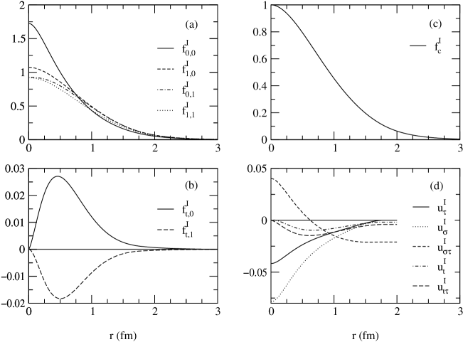
Figure 7: Internal pair correlation functions in nucleon: (a) central, projected into $T,S$ channels, $f^{I}_{T,S}$; (b) $S=1$ tensor, $f^{I}_{t,T}$; (c) central correlation, $f^{I}_{c}$; (d) operator correlations, $u^{I}_{p}=f^{I}_{p}/f^{I}_{c}$, at $r<2$. They are constant for $r>2$ fm.

The optimum internal correlations are plotted in Fig.(7). At small distances, $\lesssim 0.5$ fm the spin-isospin dependence is seen in the relative sizes of the $f^{c}_{T,S}$. We notice that $T,S=0,0$ pairs are favored at small distance due to the attractive short-range terms in the OGE and OPE interactions. This results in the $u$-quark ($d$-quark) distributions in the neutron (proton) having smaller radii than their isospin partner and gives a negative rms charge radius to the neutron, as mentioned earlier.

III.2 Two-Nucleon variational wave function

The six-quark wave function representing two uncorrelated nucleons in $T,S=0,1$ state with spin projection $M_{S}$ is given by:

$$\Phi^{NN}(M_{S}) = \sum_{{\cal P}=1}^{10}(-1)^{(1+\delta_{{\cal P},1})}\Phi^{NN}_{\cal P}(M_{S})|\mathcal{P}\rangle$$ (60)

$$\Phi^{NN}_{\cal P}(M_{S}) = \frac{1}{\sqrt{2}}\left[\Psi^{N}_{\cal P}(p,m_{1};ijk)\Psi^{N}_{\cal P}(n,m_{2};lmn)\right.$$ (61)

$$-\left.\ \ \ \Psi^{N}_{\cal P}(n,m_{1};ijk)\Psi^{N}_{\cal P}(p,m_{2};lmn)\right]^{S=1}_{M_{S}}$$

Here $\Psi^{N}_{\cal P}(p(n),m_{1};ijk)$ denotes the wave function of quarks $ijk$ in the proton (neutron) with spin projection $m_{1}$, as in Eq.(43). The quark numbers $ijk$ and $lmn$ depend upon the partition ${\cal P}$, and the full wave function $\Phi^{NN}(M_{S})$ is antisymmetric under the exchange of any quark pair. The spins inside square brackets are coupled to values indicated by the sub- and superscripts.

The variational six-quark wave function, $\Psi_{V}$ for the interacting two-nucleon state is obtained by inserting correlations in the above wave function. We consider long range correlations between the centers-of-mass of quarks $ijk$ and $lmn$, as well as correlations between the nine external quark pairs, like $il$, with one quark from each singlet. The correlations between internal quark pairs, such as $ij$ in the same singlet, are included in the nucleon wave functions $\Psi^{N}_{\cal P}(p(n),m_{1};ijk)$. The $\Psi_{V}$ is chosen as:

$$\Psi_{V}(M) = \sum_{\mathcal{P}=1}^{10}(-1)^{(1+\delta_{{\cal P},1})}\left(\mathcal{S}\prod_{q=i,j,k\atop q^{\prime}=l,m,n}\hat{F}^{E}_{qq^{\prime}}\right)\Psi^{NN}_{\cal P}(M)|\mathcal{P}\rangle\ ,$$ (62)

$$\Psi^{NN}_{\cal P}(M) = \frac{\tilde{u}(r_{\cal P})}{r_{\cal P}}Y_{0}^{0}\Phi^{NN}_{\cal P}(M_{S}=M)+\frac{\tilde{w}(r_{\cal P})}{r_{\cal P}}\left[Y_{2}^{M_{L}}(\hat{\mathbf{r}}_{\cal P})\Phi^{NN}_{\cal P}(M_{S})\right]^{J=1}_{M_{J}=M}$$ (63)

where

$${\bf r}_{\cal P}=\frac{1}{3}({\bf r}_{i}+{\bf r}_{j}+{\bf r}_{k}-{\bf r}_{l}-{\bf r}_{m}-{\bf r}_{n}).$$ (64)

The long range correlations, $\tilde{u}(r_{\cal P})$ and $\tilde{w}(r_{\cal P})$, are calculated from the two-nucleon Schrödinger equation,

$$\left\{-\frac{\hbar^{2}}{m_{N}}\nabla^{2}+\hat{v}_{NN}(\mathbf{r})\right\}\Psi^{NN}(\mathbf{r})=E^{NN}\Psi^{NN}(\mathbf{r}).$$ (65)

Here $\Psi^{NN}$ is the wave function of Eq.(63) taken in a given partition, say the first. The substitution of $\Psi^{NN}$ into Eq.(65) results in the set of coupled equations for $\tilde{u}$ and $\tilde{w}$ shown in Eqs.(1,I) with $u\to\tilde{u}$ and $w\to\tilde{w}$. These are solved subject to the boundary conditions:

$$\tilde{u}(R_{c})=0.$$

$$\tilde{w}(R_{c})=0.$$ (66)

for the ground state in a cavity of diameter $R_{c}$. The two-nucleon effective potential $\hat{v}_{NN}$, used to minimize the energy, is discussed in the next section.

The external correlation operators, $\hat{F}^{E}_{qq^{\prime}}$, contain six terms associated with the operators $O^{p=1,6}_{qq^{\prime}}$, as do the the internal correlations. By projecting the $\hat{F}^{E}_{qq^{\prime}}$ into two-quark $T,S$ channels we obtain the six functions $f^{E}_{T,S}$ and $f^{E}_{t,T}$. These functions are assumed to obey Eqs.(50–52) with the internal $v^{I}$ and $\lambda^{I}$ replaced by the external $v^{E}$ and $\lambda^{E}$, however the boundary conditions of the $f^{E}$ are different from those of $f^{I}$ as discussed below.

Terms without quark exchange between the nucleons, i.e. those having $\mathcal{P}=\mathcal{P^{\prime}}$ seem to dominate the expectation values of $\openone$ and $\hat{H}$. In these terms the confinement as well as the OGE interactions do not contribute to external pairs. Therefore we take:

$$\hat{v}^{E}_{ij}=\hat{v}^{\pi}_{ij}(\mathbf{r}_{ij}).$$ (67)

The boundary conditions for the external correlations are those appropriate for objects which are free at large separation. They are:

$$f^{E}_{T,S}(r\to 0) =$$ constant (68)

$$f^{E}_{T,S}(r\geq d_{c}) = 1$$ (69)

$$f^{E}_{t,T}(r\to 0) = 0$$ (70)

$$f^{E}_{t,T}(r\geq d_{t}) = 0$$ (71)

where $d_{c}$ and $d_{t}$ are the central and tensor “healing” lengths which are varied to minimize the variational energy.

As in the theory of nuclear matter wiringa:nm the $\lambda^{E}$ are taken as constants for distances less than the healing lengths while the boundary conditions fix the form for radii greater than the healing lengths:

$$\lambda^{E}_{T,0}(r) = \lambda^{E,0}_{T,0}\theta(d_{c}-r)+v_{T,0}\theta(r-d_{c})$$ (72)

$$\lambda^{E}_{T,1}(r) = \lambda^{E,0}_{T,1}\theta(d_{c}-r)+[v^{E}_{T,1}+\sqrt{8}(v^{E}_{t,T}-\lambda^{E}_{T,1})f_{t,T}]\theta(r-d_{c})$$ (73)

$$\lambda^{E}_{t,T}(r) = \lambda^{E,0}_{t,T}\theta(d_{t}-r)+v_{t,T}\theta(r-d_{t}),$$ (74)

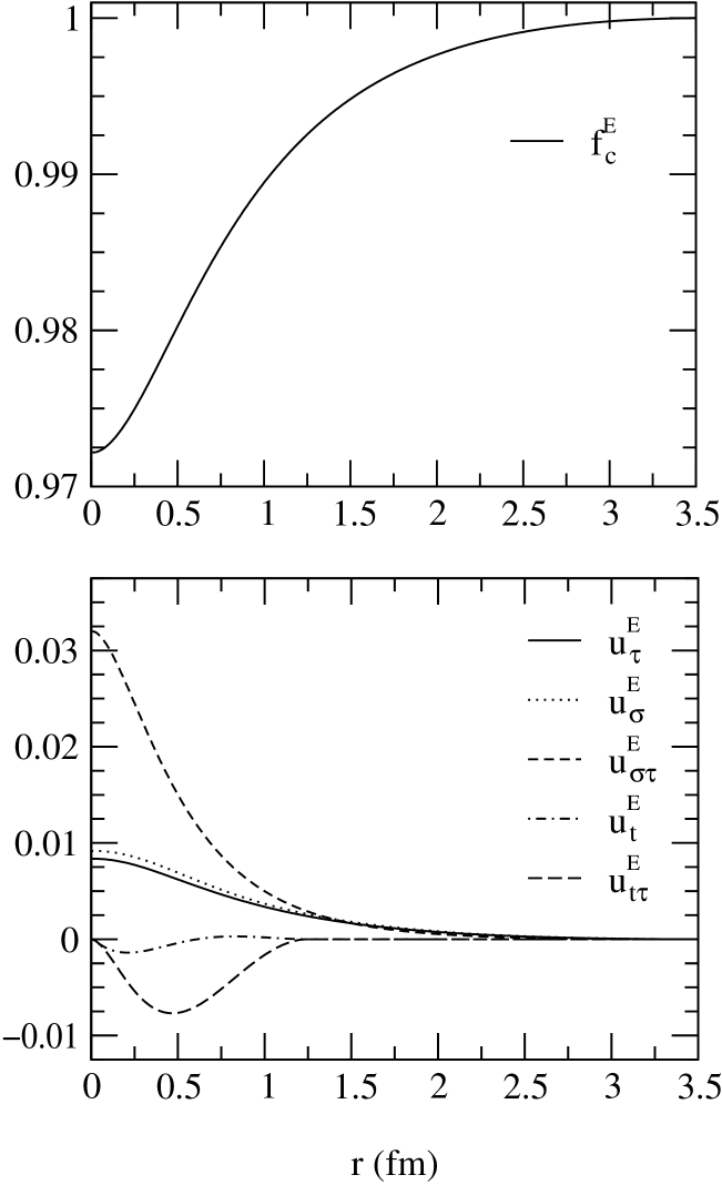
Figure 8: External pair correlation functions in six-quark wave function for $R_{c}=2$ fm with $d_{c}=3.55,d_{t}=1.25$: central correlation, $f^{E}_{c}$, (top); operator correlations, $f^{E}_{p}$ (bottom).

with $\theta(r)$ the Heaviside step function. The $\lambda^{E,0}$ are varied to match the boundary conditions, so there are no free parameters besides $d_{c}$ and $d_{t}$. The external correlations are shown in Fig.(8) for the optimum values of $d_{c},d_{t}$ at $R_{c}=2$ fm. The central correlation, $f^{E}_{c}(r)$ is seen to be $\simeq 1$ over the entire range, with a slight ‘dip’ at short distances which arises primarily due to the short-ranged $\sigma\tau$ term in OPEP. Even though the $f^{E}$ are small, they have an effect since the total wave function has a symmeterized product of nine of them.

III.3 Monte Carlo evaluation

The present VMC calculation of six-quark states is formally similar to that of ⁶Li pudliner1 except for the color factors. The wave function Eq.(62) is expressed as a vector function of the configuration vector ${\bf R}=\{{\bf r}_{1},...{\bf r}_{6}\}$:

$$\Psi_{V} = \sum_{\mathcal{P}=1}^{10}\Psi_{\cal P}({\bf R})|\mathcal{P}\rangle,$$ (75)

$$= \sum_{\mathcal{P}=1}^{10}\sum_{\alpha=1}^{320}\psi_{{\cal P},\alpha}({\bf R})|\alpha\rangle|\mathcal{P}\rangle,$$

where $|\alpha\rangle$ are six particle spin-isospin states. The tensor correlations populate all the $2^{6}$ spin states, and, since isospin is conserved, we consider only the five possible $T=0$ six-quark states. The set of the 320 states $|\alpha\rangle$ used here is the same as that in ⁶Li. In this representation the correlation operators $\hat{F}_{qq^{\prime}}$ are sparse, $320\times 320$ matrix functions of ${\bf R}$. The wave function of Eq.(62) contains symmetrized products of correlation operators $\hat{F}^{I}_{qq^{\prime}}$ and $\hat{F}^{E}_{qq^{\prime}}$. Each $\Psi_{\cal P}({\bf R})$ is a sum of $N_{pr}!$ terms, where the number of pairs, $N_{pr}=15$. The $\Psi_{\mathcal{P},r}$ denotes the term in which the $N_{pr}$ pair correlation operators act in an order denoted by $r$, and

$$\Psi_{\cal P}({\bf R})=\sum_{r=1}^{N_{pr}!}\Psi_{{\cal P},r}({\bf R}).$$ (76)

This sum is evaluated stochastically in Monte Carlo.

The expectation value of an operator:

$$\langle\hat{O}\rangle=\frac{\langle\Psi_{V}|\hat{O}|\Psi_{V}\rangle}{\langle\Psi_{V}|\Psi_{V}\rangle}=\frac{\cal N}{\cal D},$$ (77)

is evaluated using $N_{c}$ samples of ${\bf R}_{I}$, and left, right operator orders $l_{I}$ and $r_{I}$ obtained by sampling the weight:

$$W_{l,r}(\mathbf{R})=|\sum_{\mathcal{P,P^{\prime}}}(-1)^{\delta_{{\cal P},1}+\delta_{{\cal P^{\prime}},1}}\Psi_{{\cal P},l}^{\dagger}(\mathbf{R})\Psi_{{\cal P^{\prime}},r}(\mathbf{R})\langle\mathcal{P}|\mathcal{P}^{\prime}\rangle e^{-\gamma_{FT}^{2}|\mathbf{r}_{i}-\mathbf{r}_{j}|^{2}}|,$$ (78)

The average value and the standard deviation are calculated from $\sim 10^{5}$ samples using block averaging. The CD and CND contributions are evaluated separately; for example ${\cal N}={\cal N}_{CD}+{\cal N}_{CND}$, where ${\cal N}_{CD}$ is the average value of:

$$\sum_{\cal P}\Psi_{{\cal P},l_{I}}^{\dagger}(\mathbf{R}_{I})\hat{O}\Psi_{{\cal P},r_{I}}(\mathbf{R}_{I})\ ,$$ (79)

while ${\cal N}_{CND}$ contains all the other terms.

The Fortran90 computer code for this calculation was run on 6 nodes of an IBM-SP . The amount of computer time required to generate one statitistically independent configuration $\{\mathbf{R},l,r\}$ and evaluate its energy is $1.35$ node seconds. For runs of $10^{5}$ configurations, we obtain a statistical variance for the total energy of the system at the $\sim 0.1$% level. A run of this length takes $\sim 40$ node hours.

IV Six-body results

The parameters for the single particle Hamiltonian, Eq.(5), as previously described, are listed in Table 4. As mentioned earlier the $\alpha_{s}$ is determined from the $N-\Delta$ mass difference and $V_{0}$ is chosen to reproduce the nucleon mass, $m_{N}=938.9$ MeV, taken as the average of the proton and neutron masses. We choose two values for the flux-tube overlap parameter, $\gamma_{FT}$, to cover the physically interesting range, and minimize the energy of $\Psi_{V}$ with respect to variational parameters for each of them. The energy is also calculated for the $R_{c}=2$ fm case, with $\gamma_{FT}=0$, perturbatively, as discussed below.

The six-body wave function is minimized with respect to the external pair correlation operators, $\hat{F}^{E}_{ij}$, and the $NN$ long range correlation functions, $\tilde{u}$ and $\tilde{w}$. The $\hat{F}^{E}_{ij}$ are varied by adjusting the central and tensor healing lengths, $d_{c}$ and $d_{t}$. Internal pair correlation operators, $\hat{F}^{I}_{ij}$, as well as the internal triplet correlation function, $F^{I}_{123}$, are held at the equilibrium values for the single nucleon. The $\tilde{u}$ and $\tilde{w}$ in Eq.(63), are obtained from Eq.(65) with an effective $NN$ interaction, $\hat{v}_{NN}$ and subject to the boundary conditions, Eqs.(III.2). We obtain an approximate effective potential, $\hat{v}_{con}$ by the “convolution” method:

$$v_{con}(R;M)=\int d\mathbf{R}\ \delta^{(3)}\!\!\left(\mathbf{R}_{1}-\frac{R}{2}\mathbf{\hat{z}}\right)\delta^{(3)}\!\!\left(\mathbf{R}_{2}+\frac{R}{2}\mathbf{\hat{z}}\right)\Phi^{NN\dagger}_{1}(M)\left(\,\sum_{q=1,2,3}\sum_{q^{\prime}=4,5,6}\hat{v}^{\pi}_{qq^{\prime}}\right)\Phi^{NN}_{1}(M)$$ (80)

with $d\mathbf{R}=d^{3}r_{1}d^{3}r_{2}\cdots d^{3}r_{6}$, $\mathbf{R}_{1}=\frac{1}{3}(\mathbf{r}_{1}+\mathbf{r}_{2}+\mathbf{r}_{3})$, $\mathbf{R}_{2}=\frac{1}{3}(\mathbf{r}_{4}+\mathbf{r}_{5}+\mathbf{r}_{6})$, and $\Phi^{NN}_{1}$ given by Eq.(61) with $\mathcal{P}=1$. The delta-functions fix the centers-of-mass of the nucleons at separation $R$ along the $z$-axis. Note that $\Phi^{NN}_{1}$ depends only on the internal quark pairs in the first partition $\mathcal{P}=1$ and is independent of the nucleon centers-of-mass, $\mathbf{R}_{1}$ and $\mathbf{R}_{2}$. Only the OPEP between quarks in different nucleons contributes to this convolution potential; it therefore has no spin-orbit term. We evaluate $v_{con}(R;M)$ via Monte Carlo integration for two values of $M=1,0$ and project into central and tensor potentials, $v_{con}^{c}$ and $v_{con}^{t}$ as:

$$v_{con}^{c}(R) = \frac{1}{3}\left[2v_{con}(R;1)+v_{con}(R;0)\right]$$ (81)

$$v_{con}^{t}(R) = \frac{1}{6}\left[v_{con}(R;1)-v_{con}(R;0)\right].$$ (82)

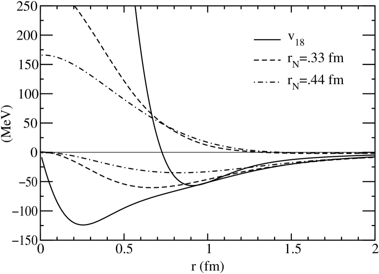
Figure 9: The $v^{c}_{d}$ and $v^{t}_{d}$ in Argonne $v_{18}$ model are compared with the $v^{c}_{con}$ and $v^{t}_{con}$ for the present $\Psi^{N}(r_{N}=0.44$ fm) and for the CKP $\Psi^{N}$ with $r_{N}=0.33$ fm.

These are plotted in Fig.(9) along with the corresponding terms from the Argonne $v_{18}$ potential which appear in Eqs.(1,I).

The effective potential appearing in Eq.(65) is taken as:

$$\hat{v}_{NN}=\alpha_{c}v_{con}^{c}+\alpha_{t}v_{con}^{t}S_{12}.$$ (83)

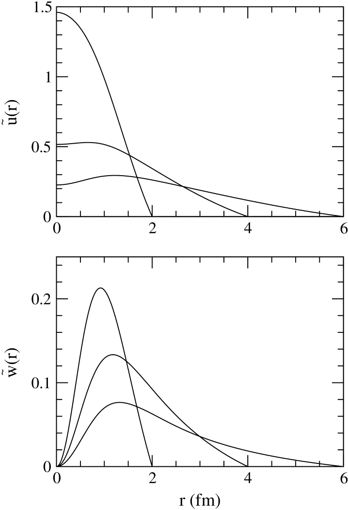
Figure 10: $NN$ radial correlation functions $\tilde{u}(r)$ (upper part) and $\tilde{w}(r)$ (lower part) for $R_{c}=2$, 4, and 6 fm.

where $\alpha_{c}$ and $\alpha_{t}$ are determined variationally for each $R_{c}$ and $\gamma_{FT}$. The resulting $\tilde{u}$ and $\tilde{w}$ for $\gamma_{FT}=2$ fm^-1 are plotted in Fig.(10). They should not be interpreted as the $NN$ two nucleon relative wave functions since the six-quark $\Psi_{V}$ contains additional $f^{E}$ correlations. The $NN$ radial wave functions may be obtained from $\Psi_{V}$ and $\Psi^{NN}$, as discussed in Sec.V. Table 5 gives the optimum values of $d_{c}$, $d_{t}$, $\alpha_{c}$, and $\alpha_{t}$. As discussed later, our $\Psi_{V}$ is less accurate for $R_{c}=6$ fm, $\gamma_{FT}\to\infty$ than for all other cases. The $\alpha_{c}$ and $\alpha_{t}$ for this case may not be the optimum values.

Smaller values of $\alpha_{c}$ are favored presumably because the external pair correlation function, $f^{E}_{c}(r_{ij})$, less than one for small distances, supresses configurations where the quarks in different nucleons approach each other. When the nucleons overlap the small difference in $f^{E}_{c}(r_{ij})$ from unity has a significant effect on the wave function since it contributes via all the nine pairs of quarks belonging to different nucleons. The facts, that $\alpha_{t}\approx 1$ in all states and $d_{t}$ is small, suggest that most of the tensor two-nucleon correlation is induced by the effective $\hat{v}_{NN}$.

The results of the full VMC calculation are given in Table 2 for each $R_{c}$ and $\gamma_{FT}$. The top three rows of this table give the total, kinetic, and potential energies for the optimum $\Psi_{V}$ per nucleon. The statistical variance relative to the total energy is:

$$\sigma_{rel}=\left(\frac{N_{c}^{-1}\sum_{I}E_{V}^{2}(\mathbf{R}_{I})-\overline{E_{V}}^{2}}{\overline{E_{V}}^{2}}\right)^{1/2}=\sqrt{\overline{\epsilon^{2}}}$$ (84)

where $E_{V}(\mathbf{R}_{I})$ is the local energy, Eq.(4), $\overline{E_{V}}$ is the average of the local energy, and $N_{c}$ is the number of configurations, $\mathbf{R}_{I}$. The relative fluctuation, $\epsilon(\mathbf{R}_{I})$, in $E_{V}(\mathbf{R}_{I})$ is defined as $E_{V}(\mathbf{R}_{I})=\overline{E_{V}}(1+\epsilon(\mathbf{R}_{I}))$, and $\sigma_{rel}$ gives its rms value. If $\Psi_{V}$ is the true ground state wave function then $E_{V}(\mathbf{R}_{I})=\overline{E_{V}}$, for all $\mathbf{R}_{I}$ and $\epsilon=0$. The rms value of $\epsilon$ is $0.13$ in all states in Table 2 except $\gamma_{FT}\to\infty$, $R_{c}=6$ fm where $\sigma_{rel}=0.17$. The perturbation calculation, $R_{c}=2$ fm, $\gamma_{FT}=0$ has $\sigma_{rel}=0.19$. We can probably reduce these $\epsilon$ values by reoptimizing $\alpha_{c}$, $\alpha_{t}$, $d_{c}$, and $d_{t}$, but the present results serve to indicate the role of the external $f^{E}$ and $\tilde{u}$ and $\tilde{w}$ in improving $\Psi_{V}$. The fluctuations in the kinetic and total potential energies, $T$ and $V$, relative to the total energy, are much larger, of $\sim\!1$. Although $T$ and $V$ fluctuate wildly as $\mathbf{R}_{I}$ varies, their sum, $E_{V}(\mathbf{R}_{I})$, changes little, evidence that $\Psi_{V}$ is a good representation of the true ground state, $\Psi_{0}$.

The standard deviation in the expectation values obtained from $10^{5}$ configurations is shown in parentheses for all observables in Table 2, and the deviation in $E_{V}$ is only 0.4 MeV per nucleon. This table also lists the contributions of the various potential terms in the Hamiltonian, and the energy of $\Psi_{V}$ relative to two free nucleons, per nucleon, compared to the empirical value calculated from Argonne $v_{18}$. It shows that all of the terms in the Hamiltonian differ by only a few percent from their single nucleon values, except $v^{\pi}_{t\tau}$, which is greatly enhanced. Comparison of the calculated $\delta E(R_{c})$ with $\delta E_{emp}(R_{c})$ shows that the present six-quark model does not give a sufficiently attractive strong interaction. The quark kinetic energy gives a repulsive contribution to $E(R_{c})$, while the interaction terms give a much smaller attraction. For example, at $R_{c}=2$ fm the $NN$ values for the total kinetic and potential energies per nucleon in Table 1 are 80 and $-43$ MeV, respectively, while the six-quark values are $62$ and $-3$, relative to two free nucleons. The kinetic energy is of the expected size but the potential is not attractive enough.

Comparison of $\gamma_{FT}=2$ fm^-1 and $\infty$ results indicates that the total effect of CND contributions, via flux-tube or quark exchange, forbidden for $\gamma_{FT}\to\infty$, is small and repulsive. A perturbative calculation with the $\gamma_{FT}=2$ fm^-1 wave function for $\gamma_{FT}=0$, i.e. no exchange suppression due to flux-tube overlap, gives an even higher energy of $1015.0(6)$ MeV/nucleon at $R_{c}=2$ fm, corresponding to $E(R_{c})=76.1(7)$ MeV/nucleon and $\delta E(R_{c})=24.9(7)$ MeV/nucleon. We breakdown the expectation values of operators into CD and CND terms, listed in Tables 6,7 and 8, according to:

$$\langle\hat{O}\rangle=\frac{\mathcal{N}_{CD}+\mathcal{N}_{CND}}{\mathcal{D}_{CD}+\mathcal{D}_{CND}}$$ (85)

where the terms in the numerator and denominator are evaluated as in Sec.III.3. The CND term of the unit operator, $\mathcal{D}_{CND}$, is small so we expand the denominator of Eq.(85) and obtain the CD contribution as $\mathcal{N}_{CD}/\mathcal{D}_{CD}$, while the CND part of the expectation value is:

$$\frac{\mathcal{N}_{CND}}{\mathcal{D}_{CD}}-\frac{\mathcal{D}_{CND}}{\mathcal{D}_{CD}}\frac{\mathcal{N}_{CD}}{\mathcal{D}_{CD}}.$$ (86)

As can be seen from Tables 6 to 8, the variance of the CD and CND contributions to the energy is larger than that of the total.

For short range quark exchange, $\gamma_{FT}=2$ fm^-1, the CND contribution of the unit operator, $\mathcal{D}_{CND}$, is $-0.0142$, $-0.0017$, and $-0.0003$ with the wave function normalized to one, for $R_{c}=2$, 4, and 6 fm, respectively. However, the sign of the $\mathcal{D}_{CND}$ changes for long range quark exchange, $\gamma_{FT}=0$, $R_{c}=2$ fm, having the value $+0.0058$. It is simple to understand why the exchange contribution is expected to be small and positive for long range quark exchange, so we consider this case first. If we ignore all spatial correlation of quarks in the wave function $\Phi^{NN}(M_{S})$ of Eq.(60), we obtain a CND contribution of $+1/9$ to the normalization. Localization of the nucleons reduces this value by suppression of exchanges for separations of the exchanged pair larger than the single nucleon rms quark diameter.

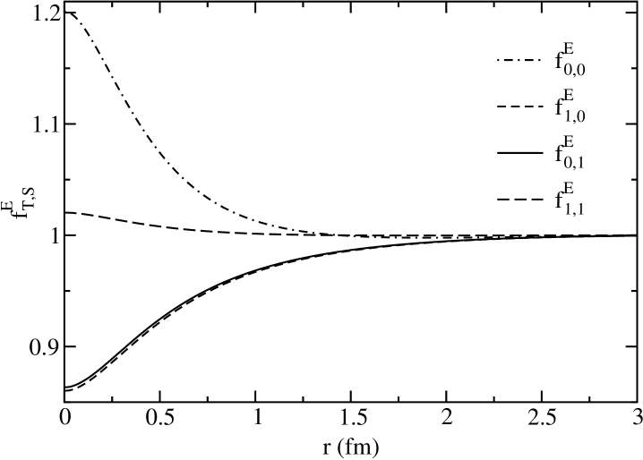
Figure 11: External central correlation operators projected into $T,S$ channels.

In the case of $\gamma_{FT}=2$ fm^-1 the sign of the CND contribution to the normalization is a consequence of the spin-isospin-color dependence of the wave function. Overall antisymmetry of the wave function implies that the sign of the contribution for exchanged quark pairs in the $T,S=(0,0)$ and $(1,1)$ states is negative while those in $(1,0)$ and $(0,1)$ are positive. External quark pairs interact via OPEP, cf. Eq.(67), resulting in the strong spin-isospin dependence of the external pair correlation functions, $f^{E}_{T,S}$, shown in Fig.(11). The $\hat{v}^{\pi}_{ij}$ is attractive at short range in $T,S=(0,0)$ and $(1,1)$ states resulting in the enhancement of exchanges which make negative contributions to the CND normalization. Similar reasoning shows that the exchange contribution due to $T,S=(1,0)$ and $(0,1)$ pairs is suppressed.

Though the quark exchange contributions are $<1\%$ of $E_{V}$, they are $\sim 10\%$ of the $E(R_{c})$, which is related to the two-nucleon interaction, and add to its repulsive core. They significantly effect the total effect of strong interactions, being the same order as $\delta E(R_{c})$.

V Conclusions

We have shown that it is possible to obtain a variational wave function for the six-quark system which gives a small standard deviation in the energy for relatively modest amounts of computational time. The present study also shows that exact calculations with small statistical errors are possible with this Hamiltonian. A GFMC code is currently being developed to project out the true ground state component of $\Psi_{V}$ using Euclidean propagation, $\Psi_{0}=\lim_{\tau\to\infty}e^{-(\hat{H}-E_{0})\tau}\Psi_{V}$.

This study also highlights the need for an improved CQM Hamiltonian. A primary issue is the inclusion of relativistic effects. The relativistic kinetic energy, $\hat{T}=\sum_{i}\sqrt{\mathbf{p}_{i}^{2}+m_{i}^{2}}$ is easy to include. Boosting the two-body potentials has been studied by Carlson et. al.carlson:rel and Forest et. al.forest:rel1 in the context of light nuclei, and by Isgur isgur:rel in a CQM. The relativization of the current model may have a significant effect on the six-quark $NN$ state. One consequence of including relativistic kinetic energy, as shown in CKP, is that with it nucleons have a smaller rms quark radius. Using the parametrization for $\Psi^{N}$ from CKP, we obtain an rms radius of 0.33 fm, against the 0.44 fm of the present $\Psi^{N}$. This has a significant effect on the convolution potential, Eq.(80), as seen in Fig.(9). As the rms quark radius of the nucleon goes to smaller values the central term of the convolution potential gets more repulsive near $r\sim 0$ and, more importantly, the tensor gets stronger. Fig.(9) shows the convolution potential tending toward the Argonne $v_{18}$ curves as the nucleon quark radius decreases.

The meson exchange picture, correct when nucleons are at large separation, is questionable when the nucleons overlap considerably. While the $v^{\pi,LR}_{\sigma\tau}$ and $v^{\pi}_{t\tau}$ are fixed by the data, the validity of $v^{\pi,SR}_{\sigma\tau}$ is questionable. As seen from the tables, this term gives a large repulsive contribution to $\delta E(R_{c})$ and one of the ways to get better agreement with $\delta E_{emp}(R_{c})$ may be to reduce its strength.

Accepting the limitations of the present model and calculations we can add terms to the six-quark Hamiltonian to reproduce the $\delta E_{emp}(R_{c})$. For example, if we assume quark pairs interact via a medium range attractive scalar potential $v^{S}$ of the two-pion exchange range:

$$v^{S} = c^{S}\sum_{q<q^{\prime}\leq 6}\tilde{T}_{\mu}^{2}(r_{qq^{\prime}})$$ (87)

$$\tilde{T}_{\mu} = T_{\mu}-\frac{\Lambda_{S}^{3}}{\mu^{3}}T_{\Lambda_{S}}-\frac{1}{2}\frac{\Lambda_{S}}{\mu}\left(\frac{\Lambda_{S}^{2}}{\mu^{2}}-1\right)\left(\Lambda_{S}r+1\right)Y_{\Lambda_{S}},$$

its strength $c^{S}$ and cutoff $\Lambda_{S}$ can be adjusted to fit $\delta E_{emp}(R_{c})$. As before $\mu$ is the pion mass. The two-pion exchange interaction between quarks has recently been discussed by Riska and Brown brown99 . The effect of this potential is calculated perturbatively from the two-quark distribution functions,

$$\rho_{2}(r)=\frac{\int\>d\mathbf{R}\Psi_{V}^{\dagger}(\mathbf{R})\sum_{q<q^{\prime}}\delta^{(3)}\!\left(\mathbf{r}-(\mathbf{r}_{i}-\mathbf{r}_{j})\right)\Psi_{V}(\mathbf{R})}{\int d\mathbf{R}\Psi_{V}^{\dagger}(\mathbf{R})\Psi_{V}(\mathbf{R})}$$ (88)

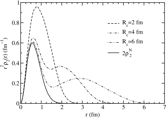
Figure 12: Quark pair distribution functions in six-quark and single nucleon states. The $\rho_{2}^{N}$ of the nucleon is multiplied by a factor of two for easier comparision.

which give the probability to find two quarks a distance $r$ apart. They are plotted in Fig.(12) for $R_{c}=2$, 4, and 6 fm. The expectation values of $v^{S}$ are given by:

$$\langle v^{S}\rangle=\int d^{3}r\rho_{2}(r)v^{S}(r).$$ (89)

The results of this exploratory calculation are shown in Table 9 for $\Lambda_{S}=5$ fm^-1 and $c^{S}$ chosen to reproduce $\delta E_{emp}(R_{c}=2$ fm). The $\langle v^{S}\rangle$ in the single nucleon state is $-51.4$ MeV and $-21.0$ MeV, for $\Lambda=5$ and 2 fm^-1 cases, respectively, which is small enough to be treated perturbatively, and it merely redefines the constant $V_{0}$. Though the effect of $v^{S}$ is minimal on the single hadron spectrum, it is larger in the six-quark case since there are nine pairs of quarks in different nucleons. This illustrates how we could refine the CQM Hamiltonian using $NN$ scattering data.

The quark pair distribution function in a single nucleon, $\rho^{N}_{2}(r)$, is also plotted in Fig.(12), scaled by a factor of 2 for easier comparison with the $\rho_{2}$ for six quarks. When $R_{c}=4$ and 6 fm the first peak in $\rho_{2}$ at $r\sim 0.6$ fm corresponds to the distribution of pairs in a single nucleon while the second peak at larger radii corresponds to the distribution of pairs of quarks in different nucleons. In these cases the first peak approximately equals $2\rho^{N}_{2}(r)$ as expected. For $R_{c}=2$ fm these peaks merge.

Further insight into the quark substructure of the two-nucleon states is gained by calculating the quark-pair distribution function for the $\mathsf{T}_{q}\cdot\mathsf{T}_{q^{\prime}}$ operator in OGE interactions. It is denoted by, $\rho^{g}_{2}$, and defined as:

$$\rho^{g}_{2}(r)=\frac{\int\>d\mathbf{R}\Psi_{V}^{\dagger}(\mathbf{R})\sum_{q<q^{\prime}}\mathsf{T}_{q}\cdot\mathsf{T}_{q^{\prime}}\delta^{(3)}\!\left(\mathbf{r}-(\mathbf{r}_{q}-\mathbf{r}_{q^{\prime}})\right)\Psi_{V}(\mathbf{R})}{\int d\mathbf{R}\Psi_{V}^{\dagger}(\mathbf{R})\Psi_{V}(\mathbf{R})}$$ (90)

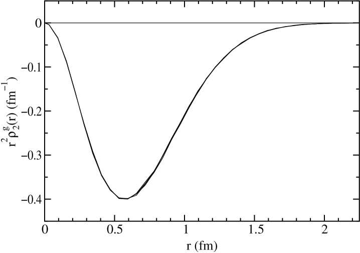
Figure 13: The quark pair $\mathsf{T}_{q^{\prime}}\cdot\mathsf{T}_{q}$ distribution function in $R_{c}=2$, 4, and 6 fm six-quark states and in the nucleon. The nucleon $\rho_{2}^{g}(r)$ is multiplied by two for easier comparison. This figure has four essentially overlapping curves.

and plotted in Fig.(13). The figure has four overlapping curves showing $\rho^{g}_{2}$ for $R_{c}=2$, 4, 6 fm and $2\rho^{g(N)}_{2}$ in the single nucleon. The $\mathsf{T}_{q}\cdot\mathsf{T}_{q^{\prime}}$ has the value $-2/3$ for quark pairs single nucleons and is zero for CD terms when the quarks are in different nucleons. Considering only the CD terms we expect the $\rho^{g}_{2}$ to lie on top of each other for all $R_{c}$. CND contributions can cause small ($\sim 1\%$) differences in $\rho^{g}_{2}$ dependent on $R_{c}$. However the accuracy of the present calculation of $\rho^{g}_{2}(r)$ is also $\sim 1\%$. Note the absence of a second peak for $r>2$ fm indicating the lack of long-ranged color-dependent correlations, as expected.

Although we will not include the results here, the effective $NN$ wave functions may be calculated from the $\Psi_{V}$ using the methods of Schiavilla et. al.schiavilla and Forest et. al.donuts , and the knowledge of $E(R_{c})$ allows one to determine $NN$ scattering phase shifts carlson:res . The aim of the present work was to explore if QMC calculations can be used to study the six-quark system with sufficient accuracy to discern nuclear effects. The present results are obviously encouraging.

$R_{c}$	2 fm	4 fm	6 fm	$\infty$
$E(R_{c})/2$	37.01	2.32	$-0.35$	$-$1.12
$\langle T_{N}(R_{c})\rangle/2$	79.61	23.96	15.16	9.94
$\langle v_{NN}(R_{c})\rangle/2$	$-$42.62	$-$21.64	$-$15.51	$-11.06$
$E_{NI}(R_{c})/2$	51.16	12.79	5.69	0
$\delta E_{emp}(R_{c})/2$	$-$14.16	$-$10.48	$-$6.04	$-1.12$

Table 1: Energies per nucleon calculated from the isoscalar part of Argonne $v_{18}$ potential (in MeV) vs. the diameter of the confining cavity. $R_{c}\to\infty$ corresponds to the free deuteron.

	$\gamma_{FT}=2$ fm-1			$\gamma_{FT}\to\infty$
$R_{c}$	2 fm	4 fm	6 fm	2 fm	4 fm	6 fm	$N$	$\Delta$
$E_{V}$	998.9(4)	950.0(4)	943.3(4)	990.7(4)	948.1(4)	942.6(5)	938.9(4)	1233.2(4)
$T$	1115(4)	1070(4)	1062(4)	1118(4)	1065(4)	1057(4)	1053(4)	755(3)
$V$	257(4)	253(4)	255(4)	247(4)	257(4)	259(4)	260(4)	852(2)
$V^{C}$	996(2)	995(2)	995(2)	997(2)	997(2)	996(2)	996(2)	1157(2)
$v^{g}_{c}$	$-$340.8(4)	$-$340.9(4)	$-$340.8(4)	$-$340.6(4)	$-$340.3(4)	$-$340.6(4)	$-$340.8(4)	$-$308.4(4)
$v^{g}_{\sigma}$	$-$101.8(3)	$-$106.5(4)	$-$107.5(4)	$-$107.0(4)	$-$106.7(4)	$-$106.9(4)	$-$107.4(4)	56.6(2)
$v^{g}_{t}$	$-$4.74(1)	$-$4.31(1)	$-$4.23(1)	$-$4.32(1)	$-$4.25(1)	$-$4.23(1)	$-$4.24(1)	$-$7.75(7)
$v^{g}_{\ell s}$	$-$2.20(1)	$-$2.09(1)	$-$2.06(1)	$-$2.24(1)	$-$2.09(1)	$-$2.07(1)	$-$2.08(1)	$-$2.28(5)
$v^{\pi,SR}_{\sigma\tau}$	$-$283(1)	$-$296(1)	$-$298(1)	$-$292(1)	$-$295(1)	$-$297(1)	$-$299(1)	$-$37.2(2)
$v^{\pi,LR}_{\sigma\tau}$	20.91(3)	22.52(4)	23.13(4)	21.51(3)	22.54(4)	23.10(5)	23.69(4)	3.96(1)
$v^{\pi}_{t\tau}$	$-$27.7(1)	$-$14.8(2)	$-$9.7(1)	$-$24.6(1)	$-$14.4(2)	$-$9.49(2)	$-$6.48(1)	$-$9.86(9)
$E(R_{c})$	60.0(6)	11.1(6)	4.4(6)	51.8(6)	9.2(6)	3.7(7)
$\delta E(R_{c})$	8.8(6)	$-$1.7(6)	$-$1.3(6)	0.7(6)	$-$3.6(6)	$-$2.0(7)
$\delta E_{emp}(R_{c})$	$-$14.21	$-$10.5	$-$6.0	$-$14.21	$-$10.5	$-$6.0

Table 2: Energies per nucleon (in MeV) of six-quark states compared with the single hadron values for single $N$ and $\Delta$. Statistical errors are shown in parenthesis.

$\mathcal{P}$	($ijk$)	($lmn$)	$P_{ij}$
1	123	456	—
2	423	156	$P_{14}$
3	523	416	$P_{15}$
4	623	451	$P_{16}$
5	143	256	$P_{24}$
6	153	426	$P_{25}$
7	163	452	$P_{26}$
8	124	356	$P_{34}$
9	125	436	$P_{35}$
10	126	453	$P_{36}$

Table 3: Six-body wave function partitions and quark exchange operators. The first column is the partition number, the second and third lists the quarks joined by flux tubes in singlets, and the last column is the quark exchange operator which gives that partition when applied to $|\mathcal{P}=1\rangle$.

$\sqrt{\sigma}$	880 MeV
$\alpha_{s}$	.61
$f_{\pi NN}/4\pi$	.075
$m_{Q}$	313 MeV
$\Lambda$	5 fm-1
$\gamma_{FT}$	2,$\infty$ fm-1
$V_{0}$	373.7 MeV

Table 4: CQM Hamiltonian parameters

$R_{c}$	$\gamma_{FT}$(fm-1)	$\alpha_{c}$	$\alpha_{t}$	$d_{c}$ (fm)	$d_{t}$ (fm)
	2	.10	.90	3.55	1.25
2	$\infty$	.17	.90	3.35	1.10
	2	.30	1.0	10.0	1.20
4	$\infty$	.50	1.0	10.0	1.10
	2	.90	.93	10.0	1.20
6	$\infty$	.34	.72	10.0	1.20

Table 5: Optimum values of the variational parameters.

	$\gamma_{FT}=2$ fm-1			$\gamma_{FT}\to\infty$	$\gamma_{FT}=0$
	CD	CND	Total	Total	CD	CND	Total
$E_{V}$	990.8(8)	8.1(3)	998.9(4)	990.7(4)	990.3(8)	25.1(3)	1015.0(6)
$T$	1117(4)	$-$2(1)	1115(4)	1117(4)	1113(4)	7(1)	1119(4)
$V$	247(4)	10.4(2)	257(4)	247(4)	252(3)	18.1(3)	270(3)
$V^{C}$	997(2)	$-$0.44(3)	996(2)	997(2)	1000(2)	2.1(4)	1002(2)
$v^{g}_{c}$	$-$340.5(4)	$-$.2(2)	$-$340.8(4)	$-$340.6(4)	$-$340.0(4)	$-$.5(3)	$-$340.4(4)
$v^{g}_{\sigma}$	$-$106.2(3)	4.4(2)	$-$101.8(3)	$-$107.0(4)	$-$106.0(3)	8.0(3)	$-$98.0(3)
$v^{g}_{t}$	$-$4.31(1)	$-$.43(1)	$-$4.74(1)	$-$4.33(1)	$-$4.30(1)	$-$1.40(3)	$-$5.69(2)
$v^{g}_{\ell s}$	$-$2.26(1)	.06(1)	$-$2.20(1)	$-$2.24(1)	$-$2.25(1)	.024(6)	$-$2.22(1)
$v^{\pi,SR}_{\sigma\tau}$	$-$290(1)	8.1(5)	$-$283(1)	$-$292(1)	$-$290(1)	12.9(4)	$-$277(1)
$v^{\pi,LR}_{\sigma\tau}$	21.47(3)	$-$.56(3)	20.91(3)	21.52(3)	21.44(4)	$-$1.71(6)	19.71(4)
$v^{\pi}_{t\tau}$	$-$27.35(1)	$-$.39(1)	$-$27.7(1)	$-$24.6(1)	$-$27.3(1)	$-$1.29(3)	$-$28.6(1)

Table 6: Variationally determined six-quark state energies for cavity diameter $R_{c}=2$ fm for finite ($\gamma_{FT}=2$ fm^-1) and strong ($\gamma_{FT}\to\infty$) coupling. The columns give color-diagonal, CD, color-non diagonal, CND and total contributions. The $\gamma_{FT}=0$ state is evaluated perturbatively.

	$\gamma_{FT}=2$ fm-1			$\gamma_{FT}\to\infty$
	CD	CND	Total	Total
$E_{V}$	948.8(5)	1.2(1)	950.0(4)	948.1(4)
$T$	1070(4)	$-$.3(4)	1070(4)	1065(4)
$V$	252(4)	1.5(1)	253(4)	257(4)
$V^{C}$	995(2)	.0(1)	995(2)	997(2)
$v^{g}_{c}$	$-$340.8(4)	$-$.04(9)	$-$340.9(4)	$-$340.3(4)
$v^{g}_{\sigma}$	$-$107.1(4)	.6(1)	$-$106.5(4)	$-$106.7(4)
$v^{g}_{t}$	$-$4.25(1)	$-$.06(1)	$-$4.31(1)	$-$4.25(1)
$v^{g}_{\ell s}$	$-$2.10(1)	.002(1)	$-$2.09(1)	$-$2.09(1)
$v^{\pi,SR}_{\sigma\tau}$	$-$296(1)	1.1(2)	$-$296(1)	$-$295(1)
$v^{\pi,LR}_{\sigma\tau}$	22.59(4)	$-$.07(1)	22.52(3)	22.54(3)
$v^{\pi}_{t\tau}$	$-$14.8(2)	$-$.04(1)	$-$14.8(1)	$-$14.4(2)

Table 7: Six-quark state energies for cavity diameter $R_{c}=4$ fm. Notation identical to Table 6.

	$\gamma_{FT}=2$ fm-1			$\gamma_{FT}\to\infty$
	CD	CND	Total	Total
$E_{V}$	943.1(5)	.27(3)	943.3(2)	942.6(5)
$T$	1062(4)	.0(1)	1062(4)	1057(4)
$V$	255(4)	.23(3)	255(4)	259(4)
$V^{C}$	995(2)	$-$.01(5)	995(2)	996(2)
$v^{g}_{c}$	$-$340.8(4)	.02(3)	$-$340.8(4)	$-$340.6(4)
$v^{g}_{\sigma}$	$-$107.6(4)	.12(4)	$-$107.5(4)	$-$106.9(4)
$v^{g}_{t}$	$-$4.22(1)	$-$.043(1)	$-$4.23(1)	$-$4.23(1)
$v^{g}_{\ell s}$	$-$2.06(1)	.002(1)	$-$2.06(1)	$-$2.07(1)
$v^{\pi,SR}_{\sigma\tau}$	$-$300(1)	.18(8)	$-$298(1)	$-$297(1)
$v^{\pi,LR}_{\sigma\tau}$	23.14(4)	$-$.01(1)	23.13(4)	23.10(3)
$v^{\pi}_{t\tau}$	$-$9.6(1)	$-$.007(2)	$-$9.7(1)	$-$9.49(2)

Table 8: Six-quark state energies for cavity diameter $R_{c}=6$ fm. Notation identical to Table 6.

$c^{S}(MeV)$	$\Lambda_{s}$ (fm-1)	2 fm	4 fm	6 fm
0		8.8(4)	$-$1.7(4)	$-$1.3(4)
$-$0.0077	5	$-$14.2(4)	$-$6.5(4)	$-$2.6(4)
$-$0.67	2	$-$14.2(4)	$-$11.0(4)	$-$5.1(4)
$\delta E_{emp}$		$-$14.2	$-$10.5	$-$6.0

Table 9: The $\delta E(R_{c})$ for various $c^{S}$ and $\Lambda_{S}$ compared with $\delta E_{emp}(R_{c})$ from Argonne $v_{18}$ potential.

flux

(100,100)

(0,0)(.5w,.5w) thin (-.5w,0)v1 (0,0)v2 (-.25w,.433w)v3 (-.25w,.144w)v7 (0,w-.45h)v4 (0.5w,w-.45h)v5 (.25w,.567w-.45h)v6 (.25w,.856w-.45h)v8 plainv1,v7 plainv2,v7 plainv3,v7 plainv4,v8 plainv5,v8 plainv6,v8 label=(a),l.a=-85,l.d=.1wv2

(50,50)(50,50) thin (1.1w,.275w)v12 (1.273w,.175w)v22 (1.1w-.173w,.175w)v32 (1.1w,.475w)v42 (1.273w,-.025w)v52 (1.446w,.275w)v62 (1.273w,.575w)v72 (1.1w-.173w,.575w)v82 (1.1w-.346w,.275w)v92 (1.1w-.173w,-.025w)v102 plainv22,v12 plainv32,v12 plainv42,v12 plainv22,v52 plainv22,v62 plainv32,v92 plainv32,v102 plainv42,v72 plainv42,v82 label=(b),l.a=-30,l.d=.1wv102

Figure 5: Flux tube configurations for system of six quarks consistent with gauge invariance. Fig.(a) shows the flux tubes for the two nucleon state, while (b) shows the “exotic” six-quark configuration.

Figure 6: Flux tube configurations for quark exchange. The solid lines show flux tubes for the first partition (123;456). The dashed lines show the flux configuration in the seventh partition (163;452), obtained by exchanging quarks 2 and 6.