Ground states of the Wick-Cutkosky model using light-front dynamics

Abstract

We consider the ground state in a model with scalar nucleons and a meson using the formalism of light-front dynamics. Light-front potentials for two-nucleon bound states are calculated using two approaches. First, light-front time-ordered perturbation theory is used to calculate one- and two-meson-exchange potentials. These potentials give results that agree well with the ladder and ladder plus crossed box Bethe-Salpeter spectra. Secondly, approximations that incorporate non-perturbative physics are used to calculate alternative one-meson-exchange potentials. These non-perturbative potentials give better agreement with the spectra of the full non-perturbative ground-state calculation than the perturbative potentials. For lightly-bound states, all of the approaches appear to agree with each other.

I Introduction

Recent experiments at Thomas Jefferson National Accelerator Facility have measured the $A(Q^{2})$ structure function of the deuteron for momentum transfers up to 6 (GeV/c)² [1], and measurements for $B(Q^{2})$ are planned. At such large momentum transfers, a relativistic description of the deuteron is required. One approach that gives such a description is light-front dynamics, which we will examine here. To separate the effects of the using light-front dynamics from the effects of the model, we choose to use the massive Wick-Cutkosky model. This is a “toy model” investigation, instead of the full nuclear theory calculation. Using this model, the light-front Hamiltonian approach is used to solve for the bound-state wavefunction. The results of our calculation can then be compared to other calculations done with the same model but different approaches. The simplest observable that can be compared is the relationship between the bound-state mass and the coupling constant.

The utility of the light-front dynamics was first discussed by Dirac [2]. We start by expressing the four-vector $x^{\mu}$ in terms of the light-front variables $x^{\mu}=(x^{+},x^{-},x^{1},x^{2})$, where $x^{\pm}=x^{0}\pm x^{3}$. This is simply a change of variables, but an especially convenient one. Using this coordinate system and defining the commutation relations at equal light-front time ($x^{+}=t_{\text{LF}}$), we obtain a light-front Hamiltonian [3, 4, 5]. The Hamiltonian is used in the light-front Schrödinger equation to solve for the ground state.

There are many desirable features of the light-front dynamics and the use of light-front coordinates. First of all, high-energy experiments are naturally described using light-front coordinates. The wave front of a beam of high-energy particles traveling in the (negative) three-direction is defined by a surface where $x^{+}$ is (approximately) constant. Such a beam can probe the wavefunction of a target described in terms of light-front variables [3, 6]: the Bjorken $x$ variable used to describe high-energy experiments is simply the ratio of the plus momentum of the struck constituent particle to the total plus momentum ($p^{+}$) of the bound state. Secondly, the vacuum for a theory with massive particles can be very simple on the light front. This is because all massive particles and anti-particles have positive plus momentum, and the total plus momentum is a conserved quantity. Thus, the naïve vacuum (with $p^{+}=0$) is empty, and diagrams that couple to this vacuum are zero. This greatly reduces the number of non-trivial light-front time-ordered diagrams. Thirdly, the generators of boosts in the one, two, and plus directions are kinematical, meaning they are independent of the interaction. Thus, even when the Hamiltonian is truncated, the wavefunctions will transform correctly under boosts. Thus, light-front dynamics is useful for describing form factors at high momentum transfers. A drawback of the light-front formalism is that the Hamiltonian is not manifestly rotationally invariant, since the generators of rotations about the one and two directions are dynamical. A study of the effects of the loss of rotational invariance of the excited states in the model being used here was made in Ref. [7], which shows that there is less breaking of the degeneracy in the spectrum when higher order potentials are used as opposed to lower order potentials.

There are other approaches that can be used to obtain relativistic wavefunctions and bound-state energies, including the Feynman-Schwinger representation (FSR) of the two-particle Green’s function[8] and the Bethe-Salpeter equation (BSE) [9, 10, 11, 12]. The FSR is useful since it can be constructed so it is equivalent to the Bethe-Salpeter equation using a kernel where all two-particle-to-two-particle ladder and crossed ladder diagrams are included. However, it requires a path integral to be done numerically, so it is computationally intensive to obtain an accurate answer. The FSR result is to be considered the full solution that the Bethe-Salpeter and Hamiltonian equations approximate. The BSE can be solved much quicker than the FSR, however a truncation of the BSE kernel is required, causing the BSE results to differ from the FSR results. It is well known that any finite truncation of the kernel yields bound-state wavefunctions with problems, such as the incorrect one-body limit [13]. For our scalar model the potential is always attractive, so truncation of the kernel gives binding energies that are too small [14, 15, 16]. Another approach is explicitly covariant light-front dynamics [17, 18], where manifest covariance is kept at the price of using a null-plane whose orientation is not fixed.

Here we study light-front dynamics because of its close connection to experimental observables. Using field theory, light-front potentials can be derived that give results physically equivalent to those of the Bethe-Salpeter equation. We define “physically equivalent” in section III C. Depending on the diagrams used to construct the potential, one can argue that certain potentials are physically equivalent to the Bethe-Salpeter equations with certain kernels. The best that these potentials can do is reproduce the results of the corresponding Bethe-Salpeter equations. On the other hand, light-front potentials can be constructed that attempt to incorporate non-perturbative physics. It is possible that these potentials can give results that agree with the full theory results better than the Bethe-Salpeter equation using low-order kernels. We will consider both types of potentials in this paper, and see how well they perform.

A brief discussion about the approximation used is in order. It is well known that the vacuum of the full Wick-Cutkosky model is unstable [19] due to the cubic coupling which provides the interaction. However, when the bound-state calculation is restricted to the two-particle sector, the quenched approximation is used, and the self-energy and vertex-renormalization diagrams are neglected, the theory has a well defined ground state. In this paper, we compare the results of our light-front Hamiltonian calculation to the Bethe-Salpeter and FSR calculations, both of which use the same approximations. The use of these simplifying approximations allows us to highlight the differences between the various approaches. The inclusion of the self-energy diagrams and counterterms for the light-front Hamiltonian [20] and for the FSR [21, 22] will not be discussed here.

A Outline of the paper

The objective of this paper is to obtain the bound-state energy for the ground state in our theory. In our model, neutral scalar nucleons interact via a Yukawa interaction, which is mediated by a neutral scalar meson. The light-front Hamiltonian derived from the Lagrangian is used in the light-front Schrödinger equation for a two-nucleon bound state. The rules for light-front time-ordered perturbation theory (LFTOPT) are then derived for this Schrödinger equation, along with the Feynman rules for the effective potential. All of this is discussed in more detail in section II.

The full potential for the light-front Schrödinger equation is given by an infinite sum of diagrams. Using the LFTOPT rules in section III, we derive the one-boson-exchange (OBE) and two-boson-exchange (TBE) potentials, where the diagrams that give rise to mass and vertex renormalization are not included. The two-boson-exchange stretched-box (TBE:SB) diagrams, a subset of the TBE diagrams, are used to construct the TBE:SB potential, and the utility of this potential is commented on. After the discussion of the perturbative potentials, we define several potentials in section IV which attempt to incorporate non-perturbative physics in a OBE type of potential. Three potentials are obtained by approximating the OBE potential directly (giving the symmetrized mass, instantaneous, and retarded potentials), and one potential is obtained by approximating the Bethe-Salpeter equation and reducing it to a three-dimensional equation (giving the modified-Green’s-function potential).

In section V, the potentials are used to numerically obtain the spectra, the coupling constant versus bound-state mass curves. This is done by solving the light-front Schrödinger equation with each of the truncated potentials (OBE, TBE, and TBE:SB), and the approximate potentials (symmetrized mass, instantaneous, retarded, and modified-Green’s-function). We compare these results to those in the literature obtained with other approaches.

We summarize our findings in section VI. Only a few low-order terms from the perturbative potentials are needed to approximate the results of the physically equivalent Bethe-Salpeter equations [7, 23, 24]. Since the light-front potentials are calculated without including the mass and vertex renormalization diagrams, the Bethe-Salpeter kernels used also do not include those diagrams. Since the interaction in the Wick-Cutkosky model is strictly attractive, the spectra calculated using the perturbative potentials will underestimate the the binding energy compared with the spectra for the physically equivalent Bethe-Salpeter equations. As progressively higher-order terms in the potential are kept, the spectra calculated will agree better with the BSE spectra. However, when a truncated kernel is used in the Bethe-Salpeter equation, the solutions obtained are known to be a poor approximation of the full solution [14, 15, 16], which for our theory (where no renormalization graphs are kept) is given by the Feynman-Schwinger representation of the Green’s function [8, 25]. Hence, our truncated potentials cannot give the full results. The non-perturbative approximations of the potential give spectra that more closely match the spectrum of the full solution. This suggests that these approximations are reproducing the physics more accurately than the perturbative potentials.

The conventions and notations employed in this paper are summarized in Appendix A. The conversion of the light-front Schrödinger equation into matrix form suitable for numerical evaluation is discussed in Appendix B. Azimuthal-angle integrations of the OBE potentials, which help simplify the evaluation of the bound-state wavefunctions, are given in Appendix C. The loop integrations and azimuthal-angle integrations needed for the TBE potentials are discussed in Appendix D. A check of the validity of the uncrossed approximation used in section IV D is done in Appendix E.

This study is related to the work of Sales et al. [23], who computed bound states using the light-front Hamiltonian with the OBE and TBE:SB approximations, and compared to the ladder Bethe-Salpeter equation results. Here, we consider also the effect of including the crossed graph part of the TBE potential as well as several non-perturbative approximations.

II Our model

We consider an isospin doublet of two uncharged scalars $\phi=(\phi_{1},\phi_{2})$ with mass $M$ (which we will refer to as nucleons), that couple to a third, uncharged scalar $\chi$ with mass $\mu$ (which we will refer to as a meson) by a $\phi^{2}\chi$ interaction. This is the massive extension of the Wick-Cutkosky model [26], which has been used on the light front to study scattering states [18] as well as bound states [23]. The Lagrangian is

$${\mathcal{L}} = \frac{1}{2}\left(\partial_{\mu}\phi\partial^{\mu}\phi-M^{2}\phi^{2}\right)+\frac{1}{2}\left(\partial_{\mu}\chi\partial^{\mu}\chi-\mu^{2}\chi^{2}\right)+g\frac{M}{2}\phi^{2}\chi,$$ (1)

where $g$ is a dimensionless coupling constant and $\phi^{2}=\phi_{1}^{2}+\phi_{2}^{2}$.

A Light-front Hamiltonian

To obtain the light-front Hamiltonian from the Lagrangian in Eq. (1), we follow the approach used by Miller [6] and many others (see the review [3]) to write the light-front Hamiltonian ($P^{-}$) as the sum of a free, non-interacting part and a term containing the interactions. We use the conventions given in Appendix A. The operators we use can be expressed in terms of Fock space operators since for this theory in light-front dynamics, the physical vacuum is the Fock space vacuum, and thus the Hilbert space is simply the Fock space. The Hamiltonian is obtained by using the energy-momentum tensor in

$$P^{\mu}=\frac{1}{2}\int dx^{-}d^{2}x_{\perp}\;T^{+\mu}(x^{+}=0,x^{-},\mathchoice{{\hbox{\boldmath$\displaystyle x$}}}{{\hbox{\boldmath$\textstyle x$}}}{{\hbox{\boldmath$\scriptstyle x$}}}{{\hbox{\boldmath$\scriptscriptstyle x$}}}_{\perp}),$$ (2)

The usual relations determine $T^{+\mu}$, with

$$T^{\mu\nu}=-g^{\mu\nu}{\cal L}+\sum_{r}{\partial{\cal L}\over\partial(\partial_{\mu}\phi_{r})}\partial^{\nu}\phi_{r},$$ (3)

in which the degrees of freedom (the fields $\phi$ and $\chi$) are labeled by $\phi_{r}$.

It is worthwhile to consider the limit in which the interactions between the fields are removed. This will allow us to define the free Hamiltonian $P^{-}_{0}$ and to display the necessary commutation relations. The energy-momentum tensor of the non-interacting fields is defined as $T_{0}^{\mu\nu}$. Use of Eq. (3) leads to the result

$$T^{\mu\nu}_{0} = \partial^{\mu}\phi\partial^{\nu}\phi-\frac{g^{\mu\nu}}{2}\left[\partial_{\sigma}\phi\partial^{\sigma}\phi-M^{2}\phi^{2}\right]+\partial^{\mu}\chi\partial^{\nu}\chi-\frac{g^{\mu\nu}}{2}\left[\partial_{\sigma}\chi\partial^{\sigma}\chi-\mu^{2}\chi^{2}\right],$$ (4)

with

$$T^{+-}_{0}=\mathchoice{{\hbox{\boldmath$\displaystyle\nabla$}}}{{\hbox{\boldmath$\textstyle\nabla$}}}{{\hbox{\boldmath$\scriptstyle\nabla$}}}{{\hbox{\boldmath$\scriptscriptstyle\nabla$}}}_{\perp}\phi\cdot\mathchoice{{\hbox{\boldmath$\displaystyle\nabla$}}}{{\hbox{\boldmath$\textstyle\nabla$}}}{{\hbox{\boldmath$\scriptstyle\nabla$}}}{{\hbox{\boldmath$\scriptscriptstyle\nabla$}}}_{\perp}\phi+M^{2}\phi^{2}+\mathchoice{{\hbox{\boldmath$\displaystyle\nabla$}}}{{\hbox{\boldmath$\textstyle\nabla$}}}{{\hbox{\boldmath$\scriptstyle\nabla$}}}{{\hbox{\boldmath$\scriptscriptstyle\nabla$}}}_{\perp}\chi\cdot\mathchoice{{\hbox{\boldmath$\displaystyle\nabla$}}}{{\hbox{\boldmath$\textstyle\nabla$}}}{{\hbox{\boldmath$\scriptstyle\nabla$}}}{{\hbox{\boldmath$\scriptscriptstyle\nabla$}}}_{\perp}\chi+\mu^{2}\chi^{2}.$$ (5)

The scalar nucleon fields can be expressed in terms of creation and destruction operators:

$$\phi_{i}(x) = \int\frac{d^{2}k_{\perp}dk^{+}\,\theta(k^{+})}{(2\pi)^{3/2}\sqrt{2k^{+}}}\left[a_{i}(\mathchoice{{\hbox{\boldmath$\displaystyle k$}}}{{\hbox{\boldmath$\textstyle k$}}}{{\hbox{\boldmath$\scriptstyle k$}}}{{\hbox{\boldmath$\scriptscriptstyle k$}}})e^{-ik\cdot x}+a_{i}^{\dagger}(\mathchoice{{\hbox{\boldmath$\displaystyle k$}}}{{\hbox{\boldmath$\textstyle k$}}}{{\hbox{\boldmath$\scriptstyle k$}}}{{\hbox{\boldmath$\scriptscriptstyle k$}}})e^{ik\cdot x}\right],$$ (6)

where $i=1,2$ is a particle index, $k\cdot x={1\over 2}(k^{-}x^{+}+k^{+}x^{-})-\mathchoice{{\hbox{\boldmath$\displaystyle k$}}}{{\hbox{\boldmath$\textstyle k$}}}{{\hbox{\boldmath$\scriptstyle k$}}}{{\hbox{\boldmath$\scriptscriptstyle k$}}}_{\perp}\cdot\mathchoice{{\hbox{\boldmath$\displaystyle x$}}}{{\hbox{\boldmath$\textstyle x$}}}{{\hbox{\boldmath$\scriptstyle x$}}}{{\hbox{\boldmath$\scriptscriptstyle x$}}}_{\perp}$ with $k^{-}=\frac{M^{2}+\mathchoice{{\hbox{\boldmath$\displaystyle k$}}}{{\hbox{\boldmath$\textstyle k$}}}{{\hbox{\boldmath$\scriptstyle k$}}}{{\hbox{\boldmath$\scriptscriptstyle k$}}}_{\perp}^{2}}{k^{+}}$, and $\mathchoice{{\hbox{\boldmath$\displaystyle k$}}}{{\hbox{\boldmath$\textstyle k$}}}{{\hbox{\boldmath$\scriptstyle k$}}}{{\hbox{\boldmath$\scriptscriptstyle k$}}}\equiv(k^{+},\mathchoice{{\hbox{\boldmath$\displaystyle k$}}}{{\hbox{\boldmath$\textstyle k$}}}{{\hbox{\boldmath$\scriptstyle k$}}}{{\hbox{\boldmath$\scriptscriptstyle k$}}}_{\perp})$. Note that $k^{-}$ is such that the particles are on the mass shell, which is a consequence of using a Hamiltonian theory. The $\theta$ function restricts $k^{+}$ to positive values. Likewise, the scalar meson field is given by

$$\chi(x) = \int\frac{d^{2}k_{\perp}dk^{+}\,\theta(k^{+})}{(2\pi)^{3/2}\sqrt{2k^{+}}}\left[a_{\chi}(\mathchoice{{\hbox{\boldmath$\displaystyle k$}}}{{\hbox{\boldmath$\textstyle k$}}}{{\hbox{\boldmath$\scriptstyle k$}}}{{\hbox{\boldmath$\scriptscriptstyle k$}}})e^{-ik\cdot x}+a_{\chi}^{\dagger}(\mathchoice{{\hbox{\boldmath$\displaystyle k$}}}{{\hbox{\boldmath$\textstyle k$}}}{{\hbox{\boldmath$\scriptstyle k$}}}{{\hbox{\boldmath$\scriptscriptstyle k$}}})e^{ik\cdot x}\right],$$ (7)

where $k^{-}=\frac{\mu^{2}+\mathchoice{{\hbox{\boldmath$\displaystyle k$}}}{{\hbox{\boldmath$\textstyle k$}}}{{\hbox{\boldmath$\scriptstyle k$}}}{{\hbox{\boldmath$\scriptscriptstyle k$}}}_{\perp}^{2}}{k^{+}}$, so that the mesons are also on the mass shell. The non-vanishing commutation relations are

$$\left[a_{\alpha}(\mathchoice{{\hbox{\boldmath$\displaystyle k$}}}{{\hbox{\boldmath$\textstyle k$}}}{{\hbox{\boldmath$\scriptstyle k$}}}{{\hbox{\boldmath$\scriptscriptstyle k$}}}),a_{\alpha}^{\dagger}(\mathchoice{{\hbox{\boldmath$\displaystyle k$}}}{{\hbox{\boldmath$\textstyle k$}}}{{\hbox{\boldmath$\scriptstyle k$}}}{{\hbox{\boldmath$\scriptscriptstyle k$}}}^{\prime})\right] = \delta(\mathchoice{{\hbox{\boldmath$\displaystyle k$}}}{{\hbox{\boldmath$\textstyle k$}}}{{\hbox{\boldmath$\scriptstyle k$}}}{{\hbox{\boldmath$\scriptscriptstyle k$}}}_{\perp}-\mathchoice{{\hbox{\boldmath$\displaystyle k$}}}{{\hbox{\boldmath$\textstyle k$}}}{{\hbox{\boldmath$\scriptstyle k$}}}{{\hbox{\boldmath$\scriptscriptstyle k$}}}^{\prime}_{\perp})\delta(k^{+}-k^{\prime+}),$$ (8)

where $\alpha=1,2,\chi$ is a particle index. The commutation relations are defined at equal light-front time, $x^{+}=0$. It is useful to define

$$\delta^{(2,+)}(\mathchoice{{\hbox{\boldmath$\displaystyle k$}}}{{\hbox{\boldmath$\textstyle k$}}}{{\hbox{\boldmath$\scriptstyle k$}}}{{\hbox{\boldmath$\scriptscriptstyle k$}}}-\mathchoice{{\hbox{\boldmath$\displaystyle k$}}}{{\hbox{\boldmath$\textstyle k$}}}{{\hbox{\boldmath$\scriptstyle k$}}}{{\hbox{\boldmath$\scriptscriptstyle k$}}}^{\prime}) \equiv \delta(\mathchoice{{\hbox{\boldmath$\displaystyle k$}}}{{\hbox{\boldmath$\textstyle k$}}}{{\hbox{\boldmath$\scriptstyle k$}}}{{\hbox{\boldmath$\scriptscriptstyle k$}}}_{\perp}-\mathchoice{{\hbox{\boldmath$\displaystyle k$}}}{{\hbox{\boldmath$\textstyle k$}}}{{\hbox{\boldmath$\scriptstyle k$}}}{{\hbox{\boldmath$\scriptscriptstyle k$}}}^{\prime}_{\perp})\delta(k^{+}-k^{\prime+}),$$ (9)

which will be used throughout this paper.

We write a ket in the two-distinguishable-particle sector of the Fock space as

$$|k_{1},k_{2}\rangle = a_{1}^{\dagger}(k_{1})a_{2}^{\dagger}(k_{2})|0\rangle.$$ (10)

This implies that the identity operator in this Fock space sector can be written as

$$I_{2} = \int d^{2}k_{1,\perp}dk_{1}^{+}\int d^{2}k_{2,\perp}dk_{2}^{+}|k_{1},k_{2}\rangle\langle k_{1},k_{2}|.$$ (11)

The derivatives appearing in the quantity $T^{+-}_{0}$ are evaluated and then one sets $x^{+}$ to 0 to obtain the result

$$P^{-}_{0} = \int_{k}\,\left[\frac{M^{2}+\mathchoice{{\hbox{\boldmath$\displaystyle k$}}}{{\hbox{\boldmath$\textstyle k$}}}{{\hbox{\boldmath$\scriptstyle k$}}}{{\hbox{\boldmath$\scriptscriptstyle k$}}}_{\perp}^{2}}{k^{+}}\left(a_{1}^{\dagger}(k)a_{1}(k)+a_{2}^{\dagger}(k)a_{2}(k)\right)+\frac{\mu^{2}+\mathchoice{{\hbox{\boldmath$\displaystyle k$}}}{{\hbox{\boldmath$\textstyle k$}}}{{\hbox{\boldmath$\scriptstyle k$}}}{{\hbox{\boldmath$\scriptscriptstyle k$}}}_{\perp}^{2}}{k^{+}}a_{\chi}^{\dagger}(k)a_{\chi}(k)\right],$$ (12)

with $\int_{k}=\int d^{2}k_{\perp}dk^{+}\,\theta(k^{+})$. Eq. (12) has the interpretation of an operator that counts the light-front energy $k^{-}$ (which is $\frac{M^{2}+\mathchoice{{\hbox{\boldmath$\displaystyle k$}}}{{\hbox{\boldmath$\textstyle k$}}}{{\hbox{\boldmath$\scriptstyle k$}}}{{\hbox{\boldmath$\scriptscriptstyle k$}}}_{\perp}^{2}}{k^{+}}$ for the nucleons and $\frac{\mu^{2}+\mathchoice{{\hbox{\boldmath$\displaystyle k$}}}{{\hbox{\boldmath$\textstyle k$}}}{{\hbox{\boldmath$\scriptstyle k$}}}{{\hbox{\boldmath$\scriptscriptstyle k$}}}_{\perp}^{2}}{k^{+}}$ for the mesons) of all of the particles.

We now consider the interacting part of the Lagrangian, ${\mathcal{L}}_{I}$. An analysis similar to that for the non-interacting parts yields the interacting part of the light-front Hamiltonian $P_{I}^{-}$;

$$P_{I}^{-} = \sum_{i=1,2}\frac{M}{2}\int_{k}\int_{k^{\prime}}\frac{1}{(2\pi)^{3/2}\sqrt{2k^{+}k^{\prime+}(k^{+}+k^{\prime+})}}$$ (15)

$$\phantom{\sum_{i=1,2}\frac{gM}{2}\int_{k}\int_{k^{\prime}}}\times\left\{\left[2a_{i}^{\dagger}(k+k^{\prime})a_{\chi}(k^{\prime})a_{i}(k)+a_{\chi}^{\dagger}(k+k^{\prime})a_{i}(k^{\prime})a_{i}(k)\right]\right.$$

$$\phantom{\sum_{i=1,2}\frac{gM}{2}\int_{k}\int_{k^{\prime}}\times\left\{\right.}+\mbox{Hermitian conjugate}\Big{\}}.\phantom{\left.\right\}}$$

The interaction Hamiltonian is self-adjoint since the Hilbert space is the Fock space. The total light-front Hamiltonian is given by $P^{-}=P^{-}_{0}+gP^{-}_{I}$.

B Hamiltonian bound-state equations

We will be studying the bound states of two distinguishable nucleons. The technology of time-ordered (old-fashioned) perturbation theory is used to construct the light-front time-ordered perturbation theory (LFTOPT) for our Hamiltonian. We start with the light-front Schrödinger equation in the full Fock space,

$$\left(P_{0}^{-}+gP_{I}^{-}\right)|\psi^{\text{GS}}_{F}\rangle = |\psi^{\text{GS}}_{F}\rangle P^{-}_{\text{GS}},$$ (16)

where $P_{0}^{-}+gP_{I}^{-}$ is the Hamiltonian in the full Fock-space basis, $|\psi^{\text{GS}}_{F}\rangle$ is the ground-state wavefunction in the full Fock space, and $P^{-}_{\text{GS}}$ is the light-front energy of that state. Recall that $P^{-}_{0}$, the non-interacting part of the Hamiltonian, is diagonal in the momentum basis, while $P^{-}_{I}$, which contains the interaction, has only off-diagonal elements.

A serious drawback of this equation is that the wavefunction $\psi^{\text{GS}}_{F}\rangle$ has support from infinitely many sectors of the Fock space, since $P^{-}_{I}$ changes the total number of particles. However, the components of the wavefunction with many particles will be small compared to the two-particle component if the coupling constant is not too large. We will construct the two-particle light-front Schrödinger equation which the two-particle component of the wavefunction satisfies. From this construction, we will obtain the rules for the LFTOPT.

We start by introducing the projection operators ${\mathcal{P}}$ and ${\mathcal{Q}}$. The operator ${\mathcal{P}}$ projects out the sector of Fock space with two distinguishable nucleons and no mesons, while ${\mathcal{Q}}=I-{\mathcal{P}}$ projects out all the other sectors. We define

$${\mathcal{P}}|\psi^{\text{GS}}_{F}\rangle \equiv |\psi^{\text{GS}}\rangle$$ (17)

$${\mathcal{Q}}|\psi^{\text{GS}}_{F}\rangle \equiv |\psi^{\text{GS}}_{Q}\rangle,$$ (18)

so that $|\psi^{\text{GS}}_{F}\rangle=|\psi^{\text{GS}}\rangle+|\psi^{\text{GS}}_{Q}\rangle$. Since the free Hamiltonian does not change the number of particles, $[{\mathcal{P}},P_{0}^{-}]=[{\mathcal{Q}},P_{0}^{-}]=0$. The interaction Hamiltonian changes the particle number, so it cannot connect the two-particle sector to itself, thus ${\mathcal{P}}P_{I}^{-}{\mathcal{P}}=0$.

Using these projection operators, Eq. (16) can be broken up into two parts,

$$P_{0}^{-}|\psi^{\text{GS}}\rangle+g{\mathcal{P}}P_{I}^{-}{\mathcal{Q}}|\psi^{\text{GS}}_{Q}\rangle = |\psi^{\text{GS}}\rangle P^{-}_{\text{GS}}$$ (19)

$$\left(P_{0}^{-}+g{\mathcal{Q}}P_{I}^{-}{\mathcal{Q}}\right)|\psi^{\text{GS}}_{Q}\rangle+g{\mathcal{Q}}P_{I}^{-}{\mathcal{P}}|\psi^{\text{GS}}\rangle = |\psi^{\text{GS}}_{Q}\rangle P^{-}_{\text{GS}}.$$ (20)

Eliminating the $|\psi^{\text{GS}}_{Q}\rangle$ and using the expression of the identity given in Eq. (11) we obtain the two-particle effective light-front Schrödinger equation

$$\int d^{2}p_{1,\perp}dp_{1}^{+}\int d^{2}p_{2,\perp}dp_{2}^{+}\langle\mathchoice{{\hbox{\boldmath$\displaystyle k$}}}{{\hbox{\boldmath$\textstyle k$}}}{{\hbox{\boldmath$\scriptstyle k$}}}{{\hbox{\boldmath$\scriptscriptstyle k$}}}_{1},\mathchoice{{\hbox{\boldmath$\displaystyle k$}}}{{\hbox{\boldmath$\textstyle k$}}}{{\hbox{\boldmath$\scriptstyle k$}}}{{\hbox{\boldmath$\scriptscriptstyle k$}}}_{2}|\left[P_{0}^{-}+V(g,P^{-}_{\text{GS}})\right]|\mathchoice{{\hbox{\boldmath$\displaystyle p$}}}{{\hbox{\boldmath$\textstyle p$}}}{{\hbox{\boldmath$\scriptstyle p$}}}{{\hbox{\boldmath$\scriptscriptstyle p$}}}_{1},\mathchoice{{\hbox{\boldmath$\displaystyle p$}}}{{\hbox{\boldmath$\textstyle p$}}}{{\hbox{\boldmath$\scriptstyle p$}}}{{\hbox{\boldmath$\scriptscriptstyle p$}}}_{2}\rangle\langle\mathchoice{{\hbox{\boldmath$\displaystyle p$}}}{{\hbox{\boldmath$\textstyle p$}}}{{\hbox{\boldmath$\scriptstyle p$}}}{{\hbox{\boldmath$\scriptscriptstyle p$}}}_{1},\mathchoice{{\hbox{\boldmath$\displaystyle p$}}}{{\hbox{\boldmath$\textstyle p$}}}{{\hbox{\boldmath$\scriptstyle p$}}}{{\hbox{\boldmath$\scriptscriptstyle p$}}}_{2}|\psi^{\text{GS}}\rangle$$ (21)

$$\quad=\langle\mathchoice{{\hbox{\boldmath$\displaystyle k$}}}{{\hbox{\boldmath$\textstyle k$}}}{{\hbox{\boldmath$\scriptstyle k$}}}{{\hbox{\boldmath$\scriptscriptstyle k$}}}_{1},\mathchoice{{\hbox{\boldmath$\displaystyle k$}}}{{\hbox{\boldmath$\textstyle k$}}}{{\hbox{\boldmath$\scriptstyle k$}}}{{\hbox{\boldmath$\scriptscriptstyle k$}}}_{2}|\psi^{\text{GS}}\rangle P^{-}_{\text{GS}},$$ (22)

where $P_{0}^{-}$ and the potential $V$ act in the two-nucleon basis. The two-particle potential is given by

$$V(g,P^{-}) = g^{2}{\mathcal{P}}P_{I}^{-}\frac{{\mathcal{Q}}}{P^{-}-P_{0}^{-}-g{\mathcal{Q}}P_{I}^{-}{\mathcal{Q}}}P_{I}^{-}{\mathcal{P}}.$$ (23)

Note that Eq. (22) is similar to Eq. (16), except for two main differences. Here we have a two-nucleon wavefunction, which makes it simpler. However, the potential is light-front energy dependent, which makes it more complicated.

The denominator in the definition of the potential is non-diagonal in the full Fock space, so the matrix inversion that it represents is highly non-trivial. This problem is avoided by expanding the inversion in powers of the coupling constant $g$ to get

$$V(g,P^{-}) = {\mathcal{P}}P_{I}^{-}\left[\frac{g^{2}{\mathcal{Q}}}{P^{-}-P_{0}^{-}}\sum_{n=0}^{\infty}\left(P_{I}^{-}\frac{g{\mathcal{Q}}}{P^{-}-P_{0}^{-}}\right)^{n}\right]P_{I}^{-}{\mathcal{P}}.$$ (24)

This can be simplified further by noting that in the two-nucleon sector of our theory, every meson emitted must be absorbed, so there must be an even number of interactions. Thus, the full potential can be written as the sum of $n$ meson exchange potentials,

$$V(P^{-},g) = \sum_{n=1}^{\infty}g^{2n}V_{(2n)}(P^{-}),$$ (25)

where $V_{(2n)}$ is the potential due to the exchange of $n$ mesons, given by

$$V_{(2n)}(P^{-}) = {\mathcal{P}}\left(P_{I}^{-}\frac{{\mathcal{Q}}}{P^{-}-P_{0}^{-}}\right)^{2n-1}P_{I}^{-}{\mathcal{P}}.$$ (26)

It is easy to see how to write a sum of diagrams for the potential when one says what Eq. (26) represents in words. We start off with two particles, then the interaction occurs. There are two possibilities of what can happen; nucleon 1 or 2 can emit a meson. Each possibility has a separate diagram. After the interaction, there is propagation with the light-front Green’s function,

$$G_{\text{LF}}(P^{-}) = \frac{1}{P^{-}-P_{0}^{-}},$$ (27)

until another interaction occurs, and so on. We simply sum up all of the possible orderings of the interaction to get the full potential. The $n^{\text{th}}$ order potential is simply the sum of all possible diagrams with $n$-meson exchanges.

Each intermediate state in Eq. (26) has more than two particles, so the diagrams are two-particle irreducible with respect to the two-particle Green’s function $G_{2\text{LF}}={\mathcal{P}}G_{\text{LF}}{\mathcal{P}}$. We can represent $G_{2\text{LF}}$ by its diagonal matrix elements,

$$G_{2\text{LF}}(\mathchoice{{\hbox{\boldmath$\displaystyle k$}}}{{\hbox{\boldmath$\textstyle k$}}}{{\hbox{\boldmath$\scriptstyle k$}}}{{\hbox{\boldmath$\scriptscriptstyle k$}}}_{1},\mathchoice{{\hbox{\boldmath$\displaystyle k$}}}{{\hbox{\boldmath$\textstyle k$}}}{{\hbox{\boldmath$\scriptstyle k$}}}{{\hbox{\boldmath$\scriptscriptstyle k$}}}_{2};P^{-})=\frac{1}{P^{-}-k_{1}^{-}-k_{2}^{-}}.$$ (28)

In the diagrams we draw, the nucleons will be represented by solid lines and the mesons by the dashed lines. Although the states we will be considering consist of two distinguishable nucleons, we will not label the nucleon lines. We will be using the quenched approximation (so there are no nucleon loops) and neglect the mass and vertex renormalization diagrams (so the physical masses and coupling constant are used, and each meson emitted from one nucleon must be absorbed by the other nucleon). It is not expected that these restrictions will lead to qualitatively different results than the true full solution when the states are not too deeply bound. The quenched approximation is reasonable when the masses of the nucleon fields are large compared to the binding energy. Use of the physical masses and coupling constant are reasonable as well when the momenta are not too large.

We stress again that we will compare various truncations of the light-front Hamiltonian to other calculations which do not include renormalization diagrams. This is because we want to determine the effect of truncation on the light-front Hamiltonian. The differences between our calculation and those which include the self-energy graphs [20], which may be large for deeply-bound states, are not considered here.

The rules for drawing the $n$-meson-exchange graphs that correspond to this approximation are:

1. Draw all topologically distinct time-ordered diagrams with $n$ mesons. Use solid lines for the nucleons and dashed lines for the mesons.

2. Delete all graphs which couple particles to the vacuum. In the massive theory we consider here, these diagrams always vanish since the vacuum has zero plus momentum, and massive particles always have positive plus momentum.

3. Our quenched approximation and use of the physical masses and coupling constant requires us to delete all graphs that have nucleon loops or have mesons that are emitted and absorbed from the same nucleon.

4. Delete all other graphs which are not allowed in the particular approximation that is being considered. For example, consider the potential from the the Hamiltonian theory that can be obtained from the ladder Bethe-Salpeter equation. That potential will not have any graphs where the meson lines cross.

Once the diagrams are drawn, we use the following rules to convert the sum of diagrams into the potential $\langle\mathchoice{{\hbox{\boldmath$\displaystyle k$}}}{{\hbox{\boldmath$\textstyle k$}}}{{\hbox{\boldmath$\scriptstyle k$}}}{{\hbox{\boldmath$\scriptscriptstyle k$}}}_{1},\mathchoice{{\hbox{\boldmath$\displaystyle k$}}}{{\hbox{\boldmath$\textstyle k$}}}{{\hbox{\boldmath$\scriptstyle k$}}}{{\hbox{\boldmath$\scriptscriptstyle k$}}}_{2}|V_{(2n)}(P^{-})|\mathchoice{{\hbox{\boldmath$\displaystyle p$}}}{{\hbox{\boldmath$\textstyle p$}}}{{\hbox{\boldmath$\scriptstyle p$}}}{{\hbox{\boldmath$\scriptscriptstyle p$}}}_{1},\mathchoice{{\hbox{\boldmath$\displaystyle p$}}}{{\hbox{\boldmath$\textstyle p$}}}{{\hbox{\boldmath$\scriptstyle p$}}}{{\hbox{\boldmath$\scriptscriptstyle p$}}}_{2}\rangle$:

1. Overall factor of $\frac{\delta^{(2,+)}(\mathchoice{{\hbox{\boldmath$\displaystyle k$}}}{{\hbox{\boldmath$\textstyle k$}}}{{\hbox{\boldmath$\scriptstyle k$}}}{{\hbox{\boldmath$\scriptscriptstyle k$}}}_{1}+\mathchoice{{\hbox{\boldmath$\displaystyle k$}}}{{\hbox{\boldmath$\textstyle k$}}}{{\hbox{\boldmath$\scriptstyle k$}}}{{\hbox{\boldmath$\scriptscriptstyle k$}}}_{2}-\mathchoice{{\hbox{\boldmath$\displaystyle p$}}}{{\hbox{\boldmath$\textstyle p$}}}{{\hbox{\boldmath$\scriptstyle p$}}}{{\hbox{\boldmath$\scriptscriptstyle p$}}}_{1}-\mathchoice{{\hbox{\boldmath$\displaystyle p$}}}{{\hbox{\boldmath$\textstyle p$}}}{{\hbox{\boldmath$\scriptstyle p$}}}{{\hbox{\boldmath$\scriptscriptstyle p$}}}_{2})}{2(2\pi)^{3}\sqrt{k_{1}^{+}k_{2}^{+}p_{1}^{+}p_{2}^{+}}}$. This delta function says that the total light-front three-momentum is conserved. We define the light-front three-momentum $\mathchoice{{\hbox{\boldmath$\displaystyle P$}}}{{\hbox{\boldmath$\textstyle P$}}}{{\hbox{\boldmath$\scriptstyle P$}}}{{\hbox{\boldmath$\scriptscriptstyle P$}}}\equiv\mathchoice{{\hbox{\boldmath$\displaystyle k$}}}{{\hbox{\boldmath$\textstyle k$}}}{{\hbox{\boldmath$\scriptstyle k$}}}{{\hbox{\boldmath$\scriptscriptstyle k$}}}_{1}+\mathchoice{{\hbox{\boldmath$\displaystyle k$}}}{{\hbox{\boldmath$\textstyle k$}}}{{\hbox{\boldmath$\scriptstyle k$}}}{{\hbox{\boldmath$\scriptscriptstyle k$}}}_{2}$.

2. To each internal line, assign a light-front three-momentum $\mathchoice{{\hbox{\boldmath$\displaystyle q$}}}{{\hbox{\boldmath$\textstyle q$}}}{{\hbox{\boldmath$\scriptstyle q$}}}{{\hbox{\boldmath$\scriptscriptstyle q$}}}_{i}$ where $i=1,2,\ldots,N$ and $N$ is the number of internal lines. The light-front energy for particle $i$ with mass $m_{i}$ is $q_{i}=\frac{m_{1}^{2}+\mathchoice{{\hbox{\boldmath$\displaystyle q$}}}{{\hbox{\boldmath$\textstyle q$}}}{{\hbox{\boldmath$\scriptstyle q$}}}{{\hbox{\boldmath$\scriptscriptstyle q$}}}^{2}_{i,\perp}}{q_{i}^{+}}$. It is useful to define $z_{i}=q_{i}^{+}/P^{+}$.

3. A factor of $\frac{\theta(z_{i}^{+})}{z_{i}^{+}}$ for each internal line.

4. An extra factor of $\frac{M^{2}}{P^{+}P^{-}}$ for each internal meson line.

5. A factor of $\frac{P^{-}}{\left(P^{-}-\sum_{i}q_{i}^{-}\right)}$ between consecutive vertices, where the sum is over only the particles that exist in the intermediate time between those vertices.

6. Use light-front three-momentum conservation to eliminate all the independent momenta.

7. Integrate with $\int\frac{d^{2}q_{i,\perp}dz_{i}}{2P^{+}P^{-}(2\pi)^{3}}$ over all remaining free internal momenta.

8. Symmetry factor of $\frac{1}{2}$ when two nucleons are created or destroyed at the same time.

With these rules, one can calculate the effective potential for any order.

C Further development of the light-front Schrödinger equation

Once the potential is calculated, we can plug it into Eq. (22), which we as

$$\int d^{2}p_{1,\perp}dp_{1}^{+}\int d^{2}p_{2,\perp}dp_{2}^{+}\langle\mathchoice{{\hbox{\boldmath$\displaystyle k$}}}{{\hbox{\boldmath$\textstyle k$}}}{{\hbox{\boldmath$\scriptstyle k$}}}{{\hbox{\boldmath$\scriptscriptstyle k$}}}_{1},\mathchoice{{\hbox{\boldmath$\displaystyle k$}}}{{\hbox{\boldmath$\textstyle k$}}}{{\hbox{\boldmath$\scriptstyle k$}}}{{\hbox{\boldmath$\scriptscriptstyle k$}}}_{2}|\left[P_{0}^{-}+V(g(P^{-}),P^{-})\right]|\mathchoice{{\hbox{\boldmath$\displaystyle p$}}}{{\hbox{\boldmath$\textstyle p$}}}{{\hbox{\boldmath$\scriptstyle p$}}}{{\hbox{\boldmath$\scriptscriptstyle p$}}}_{1},\mathchoice{{\hbox{\boldmath$\displaystyle p$}}}{{\hbox{\boldmath$\textstyle p$}}}{{\hbox{\boldmath$\scriptstyle p$}}}{{\hbox{\boldmath$\scriptscriptstyle p$}}}_{2}\rangle\langle\mathchoice{{\hbox{\boldmath$\displaystyle p$}}}{{\hbox{\boldmath$\textstyle p$}}}{{\hbox{\boldmath$\scriptstyle p$}}}{{\hbox{\boldmath$\scriptscriptstyle p$}}}_{1},\mathchoice{{\hbox{\boldmath$\displaystyle p$}}}{{\hbox{\boldmath$\textstyle p$}}}{{\hbox{\boldmath$\scriptstyle p$}}}{{\hbox{\boldmath$\scriptscriptstyle p$}}}_{2}|\psi^{\text{GS}}\rangle$$ (29)

$$\quad=\langle\mathchoice{{\hbox{\boldmath$\displaystyle k$}}}{{\hbox{\boldmath$\textstyle k$}}}{{\hbox{\boldmath$\scriptstyle k$}}}{{\hbox{\boldmath$\scriptscriptstyle k$}}}_{1},\mathchoice{{\hbox{\boldmath$\displaystyle k$}}}{{\hbox{\boldmath$\textstyle k$}}}{{\hbox{\boldmath$\scriptstyle k$}}}{{\hbox{\boldmath$\scriptscriptstyle k$}}}_{2}|\psi^{\text{GS}}\rangle P^{-},$$ (30)

where $P^{-}$ is an arbitrary light-front energy and $g(P^{-})$ is the coupling constant which yields the bound-state wavefunction with $P^{-}$ as the bound-state energy. We call this $g(P^{-})$ the spectrum of the light-front Schrödinger equation for the corresponding wavefunction.

The total momentum $\mathchoice{{\hbox{\boldmath$\displaystyle P$}}}{{\hbox{\boldmath$\textstyle P$}}}{{\hbox{\boldmath$\scriptstyle P$}}}{{\hbox{\boldmath$\scriptscriptstyle P$}}}=\mathchoice{{\hbox{\boldmath$\displaystyle k$}}}{{\hbox{\boldmath$\textstyle k$}}}{{\hbox{\boldmath$\scriptstyle k$}}}{{\hbox{\boldmath$\scriptscriptstyle k$}}}_{1}+\mathchoice{{\hbox{\boldmath$\displaystyle k$}}}{{\hbox{\boldmath$\textstyle k$}}}{{\hbox{\boldmath$\scriptstyle k$}}}{{\hbox{\boldmath$\scriptscriptstyle k$}}}_{2}$ is conserved by the potential given in Eq. (25), so the wavefunction in Eq. (30) can be parameterized by the total momentum. To make the calculations easier later, we choose to be in the center-of-momentum frame, where the components of the total momentum can be written as $\mathchoice{{\hbox{\boldmath$\displaystyle P$}}}{{\hbox{\boldmath$\textstyle P$}}}{{\hbox{\boldmath$\scriptstyle P$}}}{{\hbox{\boldmath$\scriptscriptstyle P$}}}_{\perp}=0$ and $P^{+}=P^{-}=E$. The ground-state energy, $E$, is the same as the mass of the bound state. In terms of the binding energy $B$, $E=2M-B$. In the center-of-momentum frame, the ground-state wavefunction is parameterized by $E$, so we can define

$$\langle\mathchoice{{\hbox{\boldmath$\displaystyle k$}}}{{\hbox{\boldmath$\textstyle k$}}}{{\hbox{\boldmath$\scriptstyle k$}}}{{\hbox{\boldmath$\scriptscriptstyle k$}}}_{1},\mathchoice{{\hbox{\boldmath$\displaystyle k$}}}{{\hbox{\boldmath$\textstyle k$}}}{{\hbox{\boldmath$\scriptstyle k$}}}{{\hbox{\boldmath$\scriptscriptstyle k$}}}_{2}|\psi^{\text{GS}}_{M}\rangle = \delta^{(2,+)}(\mathchoice{{\hbox{\boldmath$\displaystyle k$}}}{{\hbox{\boldmath$\textstyle k$}}}{{\hbox{\boldmath$\scriptstyle k$}}}{{\hbox{\boldmath$\scriptscriptstyle k$}}}_{1}+\mathchoice{{\hbox{\boldmath$\displaystyle k$}}}{{\hbox{\boldmath$\textstyle k$}}}{{\hbox{\boldmath$\scriptstyle k$}}}{{\hbox{\boldmath$\scriptscriptstyle k$}}}_{2}-\mathchoice{{\hbox{\boldmath$\displaystyle P$}}}{{\hbox{\boldmath$\textstyle P$}}}{{\hbox{\boldmath$\scriptstyle P$}}}{{\hbox{\boldmath$\scriptscriptstyle P$}}})\psi^{\text{GS}}(\mathchoice{{\hbox{\boldmath$\displaystyle k$}}}{{\hbox{\boldmath$\textstyle k$}}}{{\hbox{\boldmath$\scriptstyle k$}}}{{\hbox{\boldmath$\scriptscriptstyle k$}}}_{1})$$ (31)

$$\langle\mathchoice{{\hbox{\boldmath$\displaystyle k$}}}{{\hbox{\boldmath$\textstyle k$}}}{{\hbox{\boldmath$\scriptstyle k$}}}{{\hbox{\boldmath$\scriptscriptstyle k$}}}_{1},\mathchoice{{\hbox{\boldmath$\displaystyle k$}}}{{\hbox{\boldmath$\textstyle k$}}}{{\hbox{\boldmath$\scriptstyle k$}}}{{\hbox{\boldmath$\scriptscriptstyle k$}}}_{2}|V_{(2n)}(P^{-})|\mathchoice{{\hbox{\boldmath$\displaystyle p$}}}{{\hbox{\boldmath$\textstyle p$}}}{{\hbox{\boldmath$\scriptstyle p$}}}{{\hbox{\boldmath$\scriptscriptstyle p$}}}_{1},\mathchoice{{\hbox{\boldmath$\displaystyle p$}}}{{\hbox{\boldmath$\textstyle p$}}}{{\hbox{\boldmath$\scriptstyle p$}}}{{\hbox{\boldmath$\scriptscriptstyle p$}}}_{2}\rangle = \delta^{(2,+)}(\mathchoice{{\hbox{\boldmath$\displaystyle k$}}}{{\hbox{\boldmath$\textstyle k$}}}{{\hbox{\boldmath$\scriptstyle k$}}}{{\hbox{\boldmath$\scriptscriptstyle k$}}}_{1}+\mathchoice{{\hbox{\boldmath$\displaystyle k$}}}{{\hbox{\boldmath$\textstyle k$}}}{{\hbox{\boldmath$\scriptstyle k$}}}{{\hbox{\boldmath$\scriptscriptstyle k$}}}_{2}-\mathchoice{{\hbox{\boldmath$\displaystyle p$}}}{{\hbox{\boldmath$\textstyle p$}}}{{\hbox{\boldmath$\scriptstyle p$}}}{{\hbox{\boldmath$\scriptscriptstyle p$}}}_{1}-\mathchoice{{\hbox{\boldmath$\displaystyle p$}}}{{\hbox{\boldmath$\textstyle p$}}}{{\hbox{\boldmath$\scriptstyle p$}}}{{\hbox{\boldmath$\scriptscriptstyle p$}}}_{2})V_{(2n)}(E;\mathchoice{{\hbox{\boldmath$\displaystyle k$}}}{{\hbox{\boldmath$\textstyle k$}}}{{\hbox{\boldmath$\scriptstyle k$}}}{{\hbox{\boldmath$\scriptscriptstyle k$}}}_{1};\mathchoice{{\hbox{\boldmath$\displaystyle p$}}}{{\hbox{\boldmath$\textstyle p$}}}{{\hbox{\boldmath$\scriptstyle p$}}}{{\hbox{\boldmath$\scriptscriptstyle p$}}}_{1}).$$ (32)

With these, Eq. (30) effectively becomes a one-particle equation, where particle 2’s momentum is determined by $\mathchoice{{\hbox{\boldmath$\displaystyle k$}}}{{\hbox{\boldmath$\textstyle k$}}}{{\hbox{\boldmath$\scriptstyle k$}}}{{\hbox{\boldmath$\scriptscriptstyle k$}}}_{2}=\mathchoice{{\hbox{\boldmath$\displaystyle P$}}}{{\hbox{\boldmath$\textstyle P$}}}{{\hbox{\boldmath$\scriptstyle P$}}}{{\hbox{\boldmath$\scriptscriptstyle P$}}}-\mathchoice{{\hbox{\boldmath$\displaystyle k$}}}{{\hbox{\boldmath$\textstyle k$}}}{{\hbox{\boldmath$\scriptstyle k$}}}{{\hbox{\boldmath$\scriptscriptstyle k$}}}_{1}$. The minus component (the light-front energy) of particle 2 is defined by the requirement that the particle 2 is on mass shell, so $k^{-}_{2}=(M^{2}+\mathchoice{{\hbox{\boldmath$\displaystyle k$}}}{{\hbox{\boldmath$\textstyle k$}}}{{\hbox{\boldmath$\scriptstyle k$}}}{{\hbox{\boldmath$\scriptscriptstyle k$}}}_{2,\perp}^{2})/k_{2}^{+}$. We also define $x\equiv k_{1}^{+}/P^{+}=x_{Bj}$, where $x_{Bj}$ is the Bjorken $x$ variable, so that $k_{2}^{+}/P^{+}=1-x$. Likewise, we write the Bjorken variables that correspond to the momenta $\mathchoice{{\hbox{\boldmath$\displaystyle p$}}}{{\hbox{\boldmath$\textstyle p$}}}{{\hbox{\boldmath$\scriptstyle p$}}}{{\hbox{\boldmath$\scriptscriptstyle p$}}}_{1}$ and $\mathchoice{{\hbox{\boldmath$\displaystyle q$}}}{{\hbox{\boldmath$\textstyle q$}}}{{\hbox{\boldmath$\scriptstyle q$}}}{{\hbox{\boldmath$\scriptscriptstyle q$}}}_{1}$ as $y\equiv p_{1}^{+}/P^{+}$ and $z\equiv q_{1}^{+}/P^{+}$.

Using Eqs. (31), (32), and the fact that the plus momentum of both nucleons is positive, we can write the light-front Schrödinger equation Eq. (30) as

$$\int d^{2}p_{1,\perp}\int_{0}^{E}dp^{+}_{1}V(g(E),E;\mathchoice{{\hbox{\boldmath$\displaystyle k$}}}{{\hbox{\boldmath$\textstyle k$}}}{{\hbox{\boldmath$\scriptstyle k$}}}{{\hbox{\boldmath$\scriptscriptstyle k$}}}_{1};\mathchoice{{\hbox{\boldmath$\displaystyle p$}}}{{\hbox{\boldmath$\textstyle p$}}}{{\hbox{\boldmath$\scriptstyle p$}}}{{\hbox{\boldmath$\scriptscriptstyle p$}}}_{1})\psi^{\text{GS}}(\mathchoice{{\hbox{\boldmath$\displaystyle p$}}}{{\hbox{\boldmath$\textstyle p$}}}{{\hbox{\boldmath$\scriptstyle p$}}}{{\hbox{\boldmath$\scriptscriptstyle p$}}}_{1}) = \psi^{\text{GS}}(\mathchoice{{\hbox{\boldmath$\displaystyle k$}}}{{\hbox{\boldmath$\textstyle k$}}}{{\hbox{\boldmath$\scriptstyle k$}}}{{\hbox{\boldmath$\scriptscriptstyle k$}}}_{1})(E-k_{1}^{-}-k_{2}^{-}).$$ (33)

It useful to convert from light-front coordinates $\mathchoice{{\hbox{\boldmath$\displaystyle k$}}}{{\hbox{\boldmath$\textstyle k$}}}{{\hbox{\boldmath$\scriptstyle k$}}}{{\hbox{\boldmath$\scriptscriptstyle k$}}}_{1}=(k_{1}^{+},\mathchoice{{\hbox{\boldmath$\displaystyle k$}}}{{\hbox{\boldmath$\textstyle k$}}}{{\hbox{\boldmath$\scriptstyle k$}}}{{\hbox{\boldmath$\scriptscriptstyle k$}}}_{\perp})$ to equal-time coordinates $\mathchoice{{\hbox{\boldmath$\displaystyle k$}}}{{\hbox{\boldmath$\textstyle k$}}}{{\hbox{\boldmath$\scriptstyle k$}}}{{\hbox{\boldmath$\scriptscriptstyle k$}}}_{\text{ET}}=(\mathchoice{{\hbox{\boldmath$\displaystyle k$}}}{{\hbox{\boldmath$\textstyle k$}}}{{\hbox{\boldmath$\scriptstyle k$}}}{{\hbox{\boldmath$\scriptscriptstyle k$}}}_{\perp},k^{3})$, using an implicit definition of $k^{3}$ [27]

$$k_{1}^{+} = \frac{E}{2k^{0}(\mathchoice{{\hbox{\boldmath$\displaystyle k$}}}{{\hbox{\boldmath$\textstyle k$}}}{{\hbox{\boldmath$\scriptstyle k$}}}{{\hbox{\boldmath$\scriptscriptstyle k$}}}_{\text{ET}})}\left[k^{0}(\mathchoice{{\hbox{\boldmath$\displaystyle k$}}}{{\hbox{\boldmath$\textstyle k$}}}{{\hbox{\boldmath$\scriptstyle k$}}}{{\hbox{\boldmath$\scriptscriptstyle k$}}}_{\text{ET}})+k^{3}\right]$$ (34)

$$k^{0}(\mathchoice{{\hbox{\boldmath$\displaystyle k$}}}{{\hbox{\boldmath$\textstyle k$}}}{{\hbox{\boldmath$\scriptstyle k$}}}{{\hbox{\boldmath$\scriptscriptstyle k$}}}_{\text{ET}}) = \sqrt{M^{2}+\mathchoice{{\hbox{\boldmath$\displaystyle k$}}}{{\hbox{\boldmath$\textstyle k$}}}{{\hbox{\boldmath$\scriptstyle k$}}}{{\hbox{\boldmath$\scriptscriptstyle k$}}}_{\text{ET}}^{2}}.$$ (35)

Often the explicit dependence of $k^{0}$ on $\mathchoice{{\hbox{\boldmath$\displaystyle k$}}}{{\hbox{\boldmath$\textstyle k$}}}{{\hbox{\boldmath$\scriptstyle k$}}}{{\hbox{\boldmath$\scriptscriptstyle k$}}}_{\text{ET}}$ will not be shown. It is worth emphasizing that this is just a convenient change of variables; $\psi^{\text{GS}}(\mathchoice{{\hbox{\boldmath$\displaystyle k$}}}{{\hbox{\boldmath$\textstyle k$}}}{{\hbox{\boldmath$\scriptstyle k$}}}{{\hbox{\boldmath$\scriptscriptstyle k$}}}_{\text{ET}})$ is not the usual equal-time ground-state wavefunction. With this transformation, we can express $k_{1}^{\pm}$ and $k_{2}^{\pm}$ as

$$k_{1}^{+}=k_{2}^{-}\left(\frac{E}{2k^{0}}\right)^{2}=\left(1+\frac{k^{3}}{k^{0}}\right)\frac{E}{2},$$ (37)

$$k_{2}^{+}=k_{1}^{-}\left(\frac{E}{2k^{0}}\right)^{2}=\left(1-\frac{k^{3}}{k^{0}}\right)\frac{E}{2}.$$ (38)

Using these, Eq. (33) becomes

$$\int d^{3}p_{\text{ET}}\frac{2p_{1}^{+}p_{2}^{+}}{p^{0}}V(g(E),E,\mathchoice{{\hbox{\boldmath$\displaystyle k$}}}{{\hbox{\boldmath$\textstyle k$}}}{{\hbox{\boldmath$\scriptstyle k$}}}{{\hbox{\boldmath$\scriptscriptstyle k$}}}_{\text{ET}};\mathchoice{{\hbox{\boldmath$\displaystyle p$}}}{{\hbox{\boldmath$\textstyle p$}}}{{\hbox{\boldmath$\scriptstyle p$}}}{{\hbox{\boldmath$\scriptscriptstyle p$}}}_{\text{ET}})\psi^{\text{GS}}(\mathchoice{{\hbox{\boldmath$\displaystyle p$}}}{{\hbox{\boldmath$\textstyle p$}}}{{\hbox{\boldmath$\scriptstyle p$}}}{{\hbox{\boldmath$\scriptscriptstyle p$}}}_{\text{ET}}) = \psi^{\text{GS}}(\mathchoice{{\hbox{\boldmath$\displaystyle k$}}}{{\hbox{\boldmath$\textstyle k$}}}{{\hbox{\boldmath$\scriptstyle k$}}}{{\hbox{\boldmath$\scriptscriptstyle k$}}}_{\text{ET}})\left[E^{2}-(2k^{0})^{2}\right].$$ (39)

Now consider the exchange of the particle labels 1 and 2. This causes

$$\mathchoice{{\hbox{\boldmath$\displaystyle k$}}}{{\hbox{\boldmath$\textstyle k$}}}{{\hbox{\boldmath$\scriptstyle k$}}}{{\hbox{\boldmath$\scriptscriptstyle k$}}}_{1,\perp} \rightarrow \mathchoice{{\hbox{\boldmath$\displaystyle k$}}}{{\hbox{\boldmath$\textstyle k$}}}{{\hbox{\boldmath$\scriptstyle k$}}}{{\hbox{\boldmath$\scriptscriptstyle k$}}}_{2,\perp}=-\mathchoice{{\hbox{\boldmath$\displaystyle k$}}}{{\hbox{\boldmath$\textstyle k$}}}{{\hbox{\boldmath$\scriptstyle k$}}}{{\hbox{\boldmath$\scriptscriptstyle k$}}}_{1,\perp}$$ (40)

$$k_{1}^{+} \rightarrow k_{2}^{+}=E-k_{1}^{+},$$ (41)

which means that $k^{3}$ as defined in Eq. (34) transforms as $k^{3}\rightarrow-k^{3}$, so $\mathchoice{{\hbox{\boldmath$\displaystyle k$}}}{{\hbox{\boldmath$\textstyle k$}}}{{\hbox{\boldmath$\scriptstyle k$}}}{{\hbox{\boldmath$\scriptscriptstyle k$}}}_{\text{ET}}\rightarrow-\mathchoice{{\hbox{\boldmath$\displaystyle k$}}}{{\hbox{\boldmath$\textstyle k$}}}{{\hbox{\boldmath$\scriptstyle k$}}}{{\hbox{\boldmath$\scriptscriptstyle k$}}}_{\text{ET}}$. Consequently, exchange of particle labels 1 and 2 is the same as parity for $\mathchoice{{\hbox{\boldmath$\displaystyle k$}}}{{\hbox{\boldmath$\textstyle k$}}}{{\hbox{\boldmath$\scriptstyle k$}}}{{\hbox{\boldmath$\scriptscriptstyle k$}}}_{\text{ET}}$.

Since the two nucleons are identical except for the particle label, the effective potential commutes with parity to all orders in $g^{2}$. Furthermore, the light-front Hamiltonian is explicitly invariant under rotations about the three-axis. These considerations allow us to classify the wavefunctions as eigenfunctions of parity and the three-component of the angular momentum operator. The ground state will have even parity and be invariant under rotation about the three-axis, so we can write

$$\psi^{\text{GS}}(\mathchoice{{\hbox{\boldmath$\displaystyle k$}}}{{\hbox{\boldmath$\textstyle k$}}}{{\hbox{\boldmath$\scriptstyle k$}}}{{\hbox{\boldmath$\scriptscriptstyle k$}}}_{\text{ET}})=\psi^{\text{GS}}(k_{\text{ET}},\theta_{k},\phi_{k})=\psi^{\text{GS}}(k_{\text{ET}},\theta_{k})=\psi^{\text{GS}}(k_{\text{ET}},\pi-\theta_{k}),$$ (42)

where $\theta_{k}$ and $\phi_{k}$ are the polar and azimuthal angles, respectively, for the vector $\mathchoice{{\hbox{\boldmath$\displaystyle k$}}}{{\hbox{\boldmath$\textstyle k$}}}{{\hbox{\boldmath$\scriptstyle k$}}}{{\hbox{\boldmath$\scriptscriptstyle k$}}}_{\text{ET}}$.

The cylindrical symmetry and parity of the wavefunction can be used to rewrite Eq. (39) as

$$\int_{0}^{\infty}dp_{\text{ET}}\int_{0}^{\pi/2}d\theta_{p}\frac{2p_{1}^{+}p_{2}^{+}p^{2}_{\text{ET}}\sin\theta_{p}}{p^{0}}V^{+}(k_{\text{ET}},\theta_{k};p_{\text{ET}},\theta_{p})\psi^{\text{GS}}(p_{\text{ET}},\theta_{p})$$ (43)

$$\qquad=\psi^{\text{GS}}(k_{\text{ET}},\theta_{k})\left[E^{2}-4(k^{0})^{2}\right],$$ (44)

where

$$V^{+}(k_{\text{ET}},\theta_{k};p_{\text{ET}},\theta_{p}) = \frac{1}{2}\Big{[}V(k_{\text{ET}},\theta_{k};p_{\text{ET}},\theta_{p})+V(k_{\text{ET}},\theta_{k};p_{\text{ET}},\pi-\theta_{p})\Big{]}$$ (45)

$$V(k_{\text{ET}},\theta_{k};p_{\text{ET}},\theta_{p}) = \int\!\!\!\int_{0}^{2\pi}\frac{d\phi_{k}\,d\phi_{p}}{2\pi}V(\mathchoice{{\hbox{\boldmath$\displaystyle k$}}}{{\hbox{\boldmath$\textstyle k$}}}{{\hbox{\boldmath$\scriptstyle k$}}}{{\hbox{\boldmath$\scriptscriptstyle k$}}}_{\text{ET}};\mathchoice{{\hbox{\boldmath$\displaystyle p$}}}{{\hbox{\boldmath$\textstyle p$}}}{{\hbox{\boldmath$\scriptstyle p$}}}{{\hbox{\boldmath$\scriptscriptstyle p$}}}_{\text{ET}}).$$ (46)

We call $V(k_{\text{ET}},\theta_{k};p_{\text{ET}},\theta_{p})$ the azimuthal-angle-averaged potential. The light-front vectors can also be expressed in terms of the azimuthal angle $\phi$, where $\mathchoice{{\hbox{\boldmath$\displaystyle k$}}}{{\hbox{\boldmath$\textstyle k$}}}{{\hbox{\boldmath$\scriptstyle k$}}}{{\hbox{\boldmath$\scriptscriptstyle k$}}}=(k^{+},k_{\perp},\phi_{k})$, which allows the azimuthal-angle-averaged potential to be written in light-front coordinates

$$V(k^{+}_{1},k_{1,\perp};p_{1}^{+},p_{1,\perp}) = \int\!\!\!\int_{0}^{2\pi}\frac{d\phi_{k}\,d\phi_{p}}{2\pi}V(\mathchoice{{\hbox{\boldmath$\displaystyle k$}}}{{\hbox{\boldmath$\textstyle k$}}}{{\hbox{\boldmath$\scriptstyle k$}}}{{\hbox{\boldmath$\scriptscriptstyle k$}}}_{1};\mathchoice{{\hbox{\boldmath$\displaystyle p$}}}{{\hbox{\boldmath$\textstyle p$}}}{{\hbox{\boldmath$\scriptstyle p$}}}{{\hbox{\boldmath$\scriptscriptstyle p$}}}_{1}).$$ (47)

All of the simplifications of Eq. (44) based on physical considerations have been addressed. However, further rearrangements need to be done before Eq. (44) is fit to be solved on the computer. Since these involve only numerical techniques, they are relegated to Appendix B.

III Perturbative Potentials

A truncation must be made of the expansion of the potential given in Eq. (25), since it is not feasible to calculate the infinite sum of graphs for the potential in this Hamiltonian theory. In this paper we consider three truncations of the potential derived from the field theory. First the OBE potential and the TBE potentials are calculated. Then, we note that a subset of the TBE diagrams, the stretched-box diagrams, correspond to the truncated potential derived from the ladder Bethe-Salpeter equation. Thus, three truncated potentials are obtained that have a physical interpretation.

The matrix elements of these potentials are written in the two-particle momentum basis, denoting the momentum of the incoming particles by $\mathchoice{{\hbox{\boldmath$\displaystyle p$}}}{{\hbox{\boldmath$\textstyle p$}}}{{\hbox{\boldmath$\scriptstyle p$}}}{{\hbox{\boldmath$\scriptscriptstyle p$}}}_{1}$ and $\mathchoice{{\hbox{\boldmath$\displaystyle p$}}}{{\hbox{\boldmath$\textstyle p$}}}{{\hbox{\boldmath$\scriptstyle p$}}}{{\hbox{\boldmath$\scriptscriptstyle p$}}}_{2}$, and the outgoing particles $\mathchoice{{\hbox{\boldmath$\displaystyle k$}}}{{\hbox{\boldmath$\textstyle k$}}}{{\hbox{\boldmath$\scriptstyle k$}}}{{\hbox{\boldmath$\scriptscriptstyle k$}}}_{1}$ and $\mathchoice{{\hbox{\boldmath$\displaystyle k$}}}{{\hbox{\boldmath$\textstyle k$}}}{{\hbox{\boldmath$\scriptstyle k$}}}{{\hbox{\boldmath$\scriptscriptstyle k$}}}_{2}$. For simplicity, we choose to work in the center-of-momentum frame. By inspecting the rules for converting a light-front time-ordered diagram into a potential given in section II B, and looking at Eq. (32), we find that each piece of the effective-one-particle potential $V(E;\mathchoice{{\hbox{\boldmath$\displaystyle k$}}}{{\hbox{\boldmath$\textstyle k$}}}{{\hbox{\boldmath$\scriptstyle k$}}}{{\hbox{\boldmath$\scriptscriptstyle k$}}}_{1},\mathchoice{{\hbox{\boldmath$\displaystyle p$}}}{{\hbox{\boldmath$\textstyle p$}}}{{\hbox{\boldmath$\scriptstyle p$}}}{{\hbox{\boldmath$\scriptscriptstyle p$}}}_{1})$ is proportional to

$$\frac{E}{2(2\pi)^{3}\sqrt{k_{1}^{+}k_{2}^{+}p_{1}^{+}p_{2}^{+}}}.$$ (48)

(An extra factor of $E$ is included to simplify later equations.) This term will by suppressed in all of the potentials written in this paper.

A OBE Potential

We start by drawing all the allowed and non-vanishing time-ordered diagrams with one meson exchange. These diagrams are shown in Fig. 1. The light-front time-ordered perturbation theory rules given in section II B are used to calculate the potential due to OBE potential,

$$V_{\text{OBE}}(E;\mathchoice{{\hbox{\boldmath$\displaystyle k$}}}{{\hbox{\boldmath$\textstyle k$}}}{{\hbox{\boldmath$\scriptstyle k$}}}{{\hbox{\boldmath$\scriptscriptstyle k$}}}_{1};\mathchoice{{\hbox{\boldmath$\displaystyle p$}}}{{\hbox{\boldmath$\textstyle p$}}}{{\hbox{\boldmath$\scriptstyle p$}}}{{\hbox{\boldmath$\scriptscriptstyle p$}}}_{1}) = \left(\frac{M}{E}\right)^{2}\left[\frac{\theta(x-y)/|x-y|}{E-p^{-}_{1}-k^{-}_{2}-\omega^{-}(\mathchoice{{\hbox{\boldmath$\displaystyle k$}}}{{\hbox{\boldmath$\textstyle k$}}}{{\hbox{\boldmath$\scriptstyle k$}}}{{\hbox{\boldmath$\scriptscriptstyle k$}}}_{1}-\mathchoice{{\hbox{\boldmath$\displaystyle p$}}}{{\hbox{\boldmath$\textstyle p$}}}{{\hbox{\boldmath$\scriptstyle p$}}}{{\hbox{\boldmath$\scriptscriptstyle p$}}}_{1})}\right.$$ (50)

$$\phantom{\left(\frac{M}{E}\right)^{2}\left[\right.}\left.+\frac{\theta(y-x)/|y-x|}{E-k^{-}_{1}-p^{-}_{2}-\omega^{-}(\mathchoice{{\hbox{\boldmath$\displaystyle p$}}}{{\hbox{\boldmath$\textstyle p$}}}{{\hbox{\boldmath$\scriptstyle p$}}}{{\hbox{\boldmath$\scriptscriptstyle p$}}}_{1}-\mathchoice{{\hbox{\boldmath$\displaystyle k$}}}{{\hbox{\boldmath$\textstyle k$}}}{{\hbox{\boldmath$\scriptstyle k$}}}{{\hbox{\boldmath$\scriptscriptstyle k$}}}_{1})}\right].$$

We have introduced the notation that meson with light-front three-momentum $\textstyle q$ has a light-front energy given by

$$\omega^{-}(\mathchoice{{\hbox{\boldmath$\displaystyle q$}}}{{\hbox{\boldmath$\textstyle q$}}}{{\hbox{\boldmath$\scriptstyle q$}}}{{\hbox{\boldmath$\scriptscriptstyle q$}}}) = \frac{\mu^{2}+\mathchoice{{\hbox{\boldmath$\displaystyle q$}}}{{\hbox{\boldmath$\textstyle q$}}}{{\hbox{\boldmath$\scriptstyle q$}}}{{\hbox{\boldmath$\scriptscriptstyle q$}}}_{\perp}^{2}}{q^{+}}.$$ (51)

The azimuthal-angle average of $V_{\text{OBE}}$ is discussed in Appendix C.

FIG. 1.: The diagrams for the OBE potential.

The potential given in Eq. (50) can also be used for scattering states. In that case, $E=k_{1}^{-}+k_{2}^{-}=p_{1}^{-}+p_{2}^{-}$, which allows the potential to be written as

$$V_{\text{OBE}}(E_{\text{scat}};\mathchoice{{\hbox{\boldmath$\displaystyle k$}}}{{\hbox{\boldmath$\textstyle k$}}}{{\hbox{\boldmath$\scriptstyle k$}}}{{\hbox{\boldmath$\scriptscriptstyle k$}}}_{1};\mathchoice{{\hbox{\boldmath$\displaystyle p$}}}{{\hbox{\boldmath$\textstyle p$}}}{{\hbox{\boldmath$\scriptstyle p$}}}{{\hbox{\boldmath$\scriptscriptstyle p$}}}_{1}) = \frac{M^{2}/E_{\text{scat}}}{(k_{1}-p_{1})^{2}-\mu^{2}}.$$ (52)

The scattering potential is the same as the usual equal-time OBE potential. This must be the case, since the scattering potential is also given by covariant Feynman diagrams, which have the same form independent of the form of dynamics.

Returning to the bound-state regime, we note that the OBE potential can easily be written in terms of the equal-time coordinates. A reorganization of Eq. (50) yields

$$V_{\text{OBE}}(E;\mathchoice{{\hbox{\boldmath$\displaystyle k$}}}{{\hbox{\boldmath$\textstyle k$}}}{{\hbox{\boldmath$\scriptstyle k$}}}{{\hbox{\boldmath$\scriptscriptstyle k$}}}_{\text{ET}};\mathchoice{{\hbox{\boldmath$\displaystyle p$}}}{{\hbox{\boldmath$\textstyle p$}}}{{\hbox{\boldmath$\scriptstyle p$}}}{{\hbox{\boldmath$\scriptscriptstyle p$}}}_{\text{ET}}) = \left(\frac{M}{E}\right)^{2}E\left[\frac{\theta(x-y)}{(k_{1}^{+}-p_{1}^{+})(E-p^{-}_{1}-k^{-}_{2})-\mu^{2}-(\mathchoice{{\hbox{\boldmath$\displaystyle p$}}}{{\hbox{\boldmath$\textstyle p$}}}{{\hbox{\boldmath$\scriptstyle p$}}}{{\hbox{\boldmath$\scriptscriptstyle p$}}}_{\perp}-\mathchoice{{\hbox{\boldmath$\displaystyle k$}}}{{\hbox{\boldmath$\textstyle k$}}}{{\hbox{\boldmath$\scriptstyle k$}}}{{\hbox{\boldmath$\scriptscriptstyle k$}}}_{\perp})^{2}}\right.$$ (54)

$$\phantom{\left(\frac{M}{E}\right)^{2}E\left[\right.}\left.+\frac{\theta(y-x)}{(p_{1}^{+}-k_{1}^{+})(E-k^{-}_{1}-p^{-}_{2})-\mu^{2}-(\mathchoice{{\hbox{\boldmath$\displaystyle p$}}}{{\hbox{\boldmath$\textstyle p$}}}{{\hbox{\boldmath$\scriptstyle p$}}}{{\hbox{\boldmath$\scriptscriptstyle p$}}}_{\perp}-\mathchoice{{\hbox{\boldmath$\displaystyle k$}}}{{\hbox{\boldmath$\textstyle k$}}}{{\hbox{\boldmath$\scriptstyle k$}}}{{\hbox{\boldmath$\scriptscriptstyle k$}}}_{\perp})^{2}}\right].$$

Using the relations in Eq. (II C), we find

$$(k_{1}^{+}-p_{1}^{+})(E-p^{-}_{1}-k^{-}_{2}) = \left(\frac{k^{3}}{k^{0}}-\frac{p^{3}}{p^{0}}\right)\left(\frac{E^{2}-4M^{2}}{2}-p_{\text{ET}}^{2}-k_{\text{ET}}^{2}\right)$$ (56)

$$+\frac{k^{3}}{k^{0}}\frac{p^{3}}{p^{0}}\left(k^{0}-p^{0}\right)^{2}-(k^{3}-p^{3})^{2}.$$

Under the exchange $k\leftrightarrow p$, the only thing that changes in Eq. (56) is that the first term picks up a minus sign. This observation allows Eq. (54) to be rewritten as

$$V_{\text{OBE}}(E;\mathchoice{{\hbox{\boldmath$\displaystyle k$}}}{{\hbox{\boldmath$\textstyle k$}}}{{\hbox{\boldmath$\scriptstyle k$}}}{{\hbox{\boldmath$\scriptscriptstyle k$}}}_{\text{ET}};\mathchoice{{\hbox{\boldmath$\displaystyle p$}}}{{\hbox{\boldmath$\textstyle p$}}}{{\hbox{\boldmath$\scriptstyle p$}}}{{\hbox{\boldmath$\scriptscriptstyle p$}}}_{\text{ET}}) = \left(\frac{M}{E}\right)^{2}\frac{E}{\left|\frac{k^{3}}{k^{0}}-\frac{p^{3}}{p^{0}}\right|\Delta+\frac{k^{3}}{k^{0}}\frac{p^{3}}{p^{0}}(q^{0}_{\text{ET}})^{2}-\mathchoice{{\hbox{\boldmath$\displaystyle q$}}}{{\hbox{\boldmath$\textstyle q$}}}{{\hbox{\boldmath$\scriptstyle q$}}}{{\hbox{\boldmath$\scriptscriptstyle q$}}}_{\text{ET}}^{2}-\mu^{2}},$$ (57)

where

$$\Delta = \frac{E^{2}-4M^{2}}{2}-p_{\text{ET}}^{2}-k_{\text{ET}}^{2}$$ (58)

$$q_{\text{ET}}^{\mu} = k^{\mu}_{\text{ET}}-p^{\mu}_{\text{ET}}.$$ (59)

Note that $q_{\text{ET}}^{-}$ is not the light-front energy of the meson, since in a Hamiltonian theory only the light-front three-momenta are conserved; the four-momenta is not conserved. Equation (57) will be useful in the context of approximations based on the physical arguments that we will discuss in section IV.

B TBE Potential

As in the previous section, we start by drawing all the allowed, non-vanishing time-ordered diagrams with two meson exchanges shown in Fig. 2. The diagrams are classified according to the behavior of the intermediate particles. The total TBE potential is given by the sum of all the diagrams, so

$$V_{\text{TBE}} = V_{\text{TBE:SB}}+V_{\text{TBE:SX}}+V_{\text{TBE:TX}}+V_{\text{TBE:WX}}+V_{\text{TBE:ZX}}.$$ (60)

FIG. 2.: The components of the TBE potential, (a) the stretched-box, (b) stretched-crossed, (c) T-crossed, (d) wide-crossed, and (e) Z-crossed diagrams. Here, $\widehat{q}_{1}=k_{1}+p_{1}-q_{1}$ and $\widehat{q}_{2}=k_{2}+p_{2}-q_{2}$.

In the diagrams for the TBE potential in Fig. 2, the intermediate loop momenta can be parameterized by $\mathchoice{{\hbox{\boldmath$\displaystyle q$}}}{{\hbox{\boldmath$\textstyle q$}}}{{\hbox{\boldmath$\scriptstyle q$}}}{{\hbox{\boldmath$\scriptscriptstyle q$}}}_{1}$ or $\mathchoice{{\hbox{\boldmath$\displaystyle q$}}}{{\hbox{\boldmath$\textstyle q$}}}{{\hbox{\boldmath$\scriptstyle q$}}}{{\hbox{\boldmath$\scriptscriptstyle q$}}}_{2}$. The dependent variable is defined by the relation $\mathchoice{{\hbox{\boldmath$\displaystyle P$}}}{{\hbox{\boldmath$\textstyle P$}}}{{\hbox{\boldmath$\scriptstyle P$}}}{{\hbox{\boldmath$\scriptscriptstyle P$}}}=\mathchoice{{\hbox{\boldmath$\displaystyle q$}}}{{\hbox{\boldmath$\textstyle q$}}}{{\hbox{\boldmath$\scriptstyle q$}}}{{\hbox{\boldmath$\scriptscriptstyle q$}}}_{1}+\mathchoice{{\hbox{\boldmath$\displaystyle q$}}}{{\hbox{\boldmath$\textstyle q$}}}{{\hbox{\boldmath$\scriptstyle q$}}}{{\hbox{\boldmath$\scriptscriptstyle q$}}}_{2}$. The Bjorken $x$ variable that corresponds to $\mathchoice{{\hbox{\boldmath$\displaystyle q$}}}{{\hbox{\boldmath$\textstyle q$}}}{{\hbox{\boldmath$\scriptstyle q$}}}{{\hbox{\boldmath$\scriptscriptstyle q$}}}_{1}$ ($\mathchoice{{\hbox{\boldmath$\displaystyle q$}}}{{\hbox{\boldmath$\textstyle q$}}}{{\hbox{\boldmath$\scriptstyle q$}}}{{\hbox{\boldmath$\scriptscriptstyle q$}}}_{2}$) is labeled with $z$ ($1-z$). We use the Feynman rules to calculate all of these potentials, starting with

$$V_{\text{TBE:SB}}(E;\mathchoice{{\hbox{\boldmath$\displaystyle k$}}}{{\hbox{\boldmath$\textstyle k$}}}{{\hbox{\boldmath$\scriptstyle k$}}}{{\hbox{\boldmath$\scriptscriptstyle k$}}}_{1};\mathchoice{{\hbox{\boldmath$\displaystyle p$}}}{{\hbox{\boldmath$\textstyle p$}}}{{\hbox{\boldmath$\scriptstyle p$}}}{{\hbox{\boldmath$\scriptscriptstyle p$}}}_{1}) = \left(\frac{M}{E}\right)^{4}\int\frac{d^{2}q_{\perp}}{2(2\pi)^{3}}\left[\int_{0}^{1}dz\frac{\theta(z-y)\theta(x-z)}{z(1-z)(z-y)(x-z)}\right.$$ (65)

$$\phantom{\left(\frac{M}{E}\right)^{4}\int\frac{d^{2}q_{\perp}}{2(2\pi)^{3}}\left[\right.}\left.\times\frac{1}{E-q_{1}^{-}-k_{2}^{-}-\omega^{-}(\mathchoice{{\hbox{\boldmath$\displaystyle k$}}}{{\hbox{\boldmath$\textstyle k$}}}{{\hbox{\boldmath$\scriptstyle k$}}}{{\hbox{\boldmath$\scriptscriptstyle k$}}}_{1}-\mathchoice{{\hbox{\boldmath$\displaystyle q$}}}{{\hbox{\boldmath$\textstyle q$}}}{{\hbox{\boldmath$\scriptstyle q$}}}{{\hbox{\boldmath$\scriptscriptstyle q$}}}_{1})}\right.$$

$$\phantom{\left(\frac{M}{E}\right)^{4}\int\frac{d^{2}q_{\perp}}{2(2\pi)^{3}}\left[\right.}\left.\times\frac{1}{E-p_{1}^{-}-k_{2}^{-}-\omega^{-}(\mathchoice{{\hbox{\boldmath$\displaystyle k$}}}{{\hbox{\boldmath$\textstyle k$}}}{{\hbox{\boldmath$\scriptstyle k$}}}{{\hbox{\boldmath$\scriptscriptstyle k$}}}_{1}-\mathchoice{{\hbox{\boldmath$\displaystyle q$}}}{{\hbox{\boldmath$\textstyle q$}}}{{\hbox{\boldmath$\scriptstyle q$}}}{{\hbox{\boldmath$\scriptscriptstyle q$}}}_{1})-\omega^{-}(\mathchoice{{\hbox{\boldmath$\displaystyle q$}}}{{\hbox{\boldmath$\textstyle q$}}}{{\hbox{\boldmath$\scriptstyle q$}}}{{\hbox{\boldmath$\scriptscriptstyle q$}}}_{1}-\mathchoice{{\hbox{\boldmath$\displaystyle p$}}}{{\hbox{\boldmath$\textstyle p$}}}{{\hbox{\boldmath$\scriptstyle p$}}}{{\hbox{\boldmath$\scriptscriptstyle p$}}}_{1})}\right.$$

$$\phantom{\left(\frac{M}{E}\right)^{4}\int\frac{d^{2}q_{\perp}}{2(2\pi)^{3}}\left[\right.}\left.\times\frac{1}{E-p_{1}^{-}-q_{2}^{-}-\omega^{-}(\mathchoice{{\hbox{\boldmath$\displaystyle q$}}}{{\hbox{\boldmath$\textstyle q$}}}{{\hbox{\boldmath$\scriptstyle q$}}}{{\hbox{\boldmath$\scriptscriptstyle q$}}}_{1}-\mathchoice{{\hbox{\boldmath$\displaystyle p$}}}{{\hbox{\boldmath$\textstyle p$}}}{{\hbox{\boldmath$\scriptstyle p$}}}{{\hbox{\boldmath$\scriptscriptstyle p$}}}_{1})}\right]$$

$$\phantom{\left(\frac{M}{E}\right)^{4}\int\frac{d^{2}q_{\perp}}{2(2\pi)^{3}}}+\{1\leftrightarrow 2\}.$$

The symbol $\{1\leftrightarrow 2\}$ means that all labels 1 are replaced with 2 and vice versa, as well as replacing the Bjorken variables $x$, $y$, and $z$ with $1-x$, $1-y$, and $1-z$. This is a way of explicitly stating the symmetry of the potential under exchange of particles 1 and 2. A detailed discussion of the evaluation of the loop integral in Eq. (65) is given in Appendix D.

It is straightforward to calculate the other parts of the TBE potential,

$$V_{\text{TBE:SX}}(E;\mathchoice{{\hbox{\boldmath$\displaystyle k$}}}{{\hbox{\boldmath$\textstyle k$}}}{{\hbox{\boldmath$\scriptstyle k$}}}{{\hbox{\boldmath$\scriptscriptstyle k$}}}_{1};\mathchoice{{\hbox{\boldmath$\displaystyle p$}}}{{\hbox{\boldmath$\textstyle p$}}}{{\hbox{\boldmath$\scriptstyle p$}}}{{\hbox{\boldmath$\scriptscriptstyle p$}}}_{1}) = \left(\frac{M}{E}\right)^{4}\int\frac{d^{2}q_{\perp}}{2(2\pi)^{3}}\left[\int_{0}^{1}dz\frac{\theta(x-z)\theta(z-y)}{z(x-z)(1+z-x-y)(z-y)}\right.$$ (70)

$$\phantom{\left(\frac{M}{E}\right)^{4}\int\frac{d^{2}q_{\perp}}{2(2\pi)^{3}}\left[\right.}\left.\times\frac{1}{E-q_{1}^{-}-k_{2}^{-}-\omega^{-}(\mathchoice{{\hbox{\boldmath$\displaystyle k$}}}{{\hbox{\boldmath$\textstyle k$}}}{{\hbox{\boldmath$\scriptstyle k$}}}{{\hbox{\boldmath$\scriptscriptstyle k$}}}_{1}-\mathchoice{{\hbox{\boldmath$\displaystyle q$}}}{{\hbox{\boldmath$\textstyle q$}}}{{\hbox{\boldmath$\scriptstyle q$}}}{{\hbox{\boldmath$\scriptscriptstyle q$}}}_{1})}\right.$$

$$\phantom{\left(\frac{M}{E}\right)^{4}\int\frac{d^{2}q_{\perp}}{2(2\pi)^{3}}\left[\right.}\left.\times\frac{1}{E-p_{1}^{-}-k_{2}^{-}-\omega^{-}(\mathchoice{{\hbox{\boldmath$\displaystyle k$}}}{{\hbox{\boldmath$\textstyle k$}}}{{\hbox{\boldmath$\scriptstyle k$}}}{{\hbox{\boldmath$\scriptscriptstyle k$}}}_{1}-\mathchoice{{\hbox{\boldmath$\displaystyle q$}}}{{\hbox{\boldmath$\textstyle q$}}}{{\hbox{\boldmath$\scriptstyle q$}}}{{\hbox{\boldmath$\scriptscriptstyle q$}}}_{1})-\omega^{-}(\mathchoice{{\hbox{\boldmath$\displaystyle q$}}}{{\hbox{\boldmath$\textstyle q$}}}{{\hbox{\boldmath$\scriptstyle q$}}}{{\hbox{\boldmath$\scriptscriptstyle q$}}}_{1}-\mathchoice{{\hbox{\boldmath$\displaystyle p$}}}{{\hbox{\boldmath$\textstyle p$}}}{{\hbox{\boldmath$\scriptstyle p$}}}{{\hbox{\boldmath$\scriptscriptstyle p$}}}_{1})}\right.$$

$$\phantom{\left(\frac{M}{E}\right)^{4}\int\frac{d^{2}q_{\perp}}{2(2\pi)^{3}}\left[\right.}\left.\times\frac{1}{E-p_{1}^{-}-\widehat{q}_{2}^{-}-\omega^{-}(\mathchoice{{\hbox{\boldmath$\displaystyle k$}}}{{\hbox{\boldmath$\textstyle k$}}}{{\hbox{\boldmath$\scriptstyle k$}}}{{\hbox{\boldmath$\scriptscriptstyle k$}}}_{1}-\mathchoice{{\hbox{\boldmath$\displaystyle q$}}}{{\hbox{\boldmath$\textstyle q$}}}{{\hbox{\boldmath$\scriptstyle q$}}}{{\hbox{\boldmath$\scriptscriptstyle q$}}}_{1})}\right]$$

$$\phantom{\left(\frac{M}{E}\right)^{4}\int\frac{d^{2}q_{\perp}}{2(2\pi)^{3}}}+\{1\leftrightarrow 2\},$$

where we have denoted the light-front energy of particle 2 by $\widehat{q}_{2}^{-}$, given by

$$\widehat{q}_{2}^{-} = \epsilon^{-}(\mathchoice{{\hbox{\boldmath$\displaystyle P$}}}{{\hbox{\boldmath$\textstyle P$}}}{{\hbox{\boldmath$\scriptstyle P$}}}{{\hbox{\boldmath$\scriptscriptstyle P$}}}+\mathchoice{{\hbox{\boldmath$\displaystyle q$}}}{{\hbox{\boldmath$\textstyle q$}}}{{\hbox{\boldmath$\scriptstyle q$}}}{{\hbox{\boldmath$\scriptscriptstyle q$}}}_{1}-\mathchoice{{\hbox{\boldmath$\displaystyle p$}}}{{\hbox{\boldmath$\textstyle p$}}}{{\hbox{\boldmath$\scriptstyle p$}}}{{\hbox{\boldmath$\scriptscriptstyle p$}}}_{1}-\mathchoice{{\hbox{\boldmath$\displaystyle k$}}}{{\hbox{\boldmath$\textstyle k$}}}{{\hbox{\boldmath$\scriptstyle k$}}}{{\hbox{\boldmath$\scriptscriptstyle k$}}}_{1})$$ (71)

$$\epsilon^{-}(\mathchoice{{\hbox{\boldmath$\displaystyle q$}}}{{\hbox{\boldmath$\textstyle q$}}}{{\hbox{\boldmath$\scriptstyle q$}}}{{\hbox{\boldmath$\scriptscriptstyle q$}}}) = \frac{M^{2}+\mathchoice{{\hbox{\boldmath$\displaystyle q$}}}{{\hbox{\boldmath$\textstyle q$}}}{{\hbox{\boldmath$\scriptstyle q$}}}{{\hbox{\boldmath$\scriptscriptstyle q$}}}_{\perp}^{2}}{q^{+}}.$$ (72)

The rest of the TBE potential is given by

$$V_{\text{TBE:TX}}(E;\mathchoice{{\hbox{\boldmath$\displaystyle k$}}}{{\hbox{\boldmath$\textstyle k$}}}{{\hbox{\boldmath$\scriptstyle k$}}}{{\hbox{\boldmath$\scriptscriptstyle k$}}}_{1};\mathchoice{{\hbox{\boldmath$\displaystyle p$}}}{{\hbox{\boldmath$\textstyle p$}}}{{\hbox{\boldmath$\scriptstyle p$}}}{{\hbox{\boldmath$\scriptscriptstyle p$}}}_{1}) = \left(\frac{M}{E}\right)^{4}\int\frac{d^{2}q_{\perp}}{2(2\pi)^{3}}\left[\int_{0}^{1}dz\frac{\theta(x-z)\theta(1+z-x-y)\theta(y-z)}{z(x-z)(1+z-x-y)(y-z)}\right.$$ (77)

$$\phantom{\left(\frac{M}{E}\right)^{4}\int\frac{d^{2}q_{\perp}}{2(2\pi)^{3}}\left[\right.}\left.\times\frac{1}{E-q_{1}^{-}-k_{2}^{-}-\omega^{-}(\mathchoice{{\hbox{\boldmath$\displaystyle k$}}}{{\hbox{\boldmath$\textstyle k$}}}{{\hbox{\boldmath$\scriptstyle k$}}}{{\hbox{\boldmath$\scriptscriptstyle k$}}}_{1}-\mathchoice{{\hbox{\boldmath$\displaystyle q$}}}{{\hbox{\boldmath$\textstyle q$}}}{{\hbox{\boldmath$\scriptstyle q$}}}{{\hbox{\boldmath$\scriptscriptstyle q$}}}_{1})}\right.$$

$$\phantom{\left(\frac{M}{E}\right)^{4}\int\frac{d^{2}q_{\perp}}{2(2\pi)^{3}}\left[\right.}\left.\times\frac{1}{E-q_{1}^{-}-\widehat{q}_{2}^{-}-\omega^{-}(\mathchoice{{\hbox{\boldmath$\displaystyle k$}}}{{\hbox{\boldmath$\textstyle k$}}}{{\hbox{\boldmath$\scriptstyle k$}}}{{\hbox{\boldmath$\scriptscriptstyle k$}}}_{1}-\mathchoice{{\hbox{\boldmath$\displaystyle q$}}}{{\hbox{\boldmath$\textstyle q$}}}{{\hbox{\boldmath$\scriptstyle q$}}}{{\hbox{\boldmath$\scriptscriptstyle q$}}}_{1})-\omega^{-}(\mathchoice{{\hbox{\boldmath$\displaystyle p$}}}{{\hbox{\boldmath$\textstyle p$}}}{{\hbox{\boldmath$\scriptstyle p$}}}{{\hbox{\boldmath$\scriptscriptstyle p$}}}_{1}-\mathchoice{{\hbox{\boldmath$\displaystyle q$}}}{{\hbox{\boldmath$\textstyle q$}}}{{\hbox{\boldmath$\scriptstyle q$}}}{{\hbox{\boldmath$\scriptscriptstyle q$}}}_{1})}\right.$$

$$\phantom{\left(\frac{M}{E}\right)^{4}\int\frac{d^{2}q_{\perp}}{2(2\pi)^{3}}\left[\right.}\left.\times\frac{1}{E-p_{1}^{-}-\widehat{q}_{2}^{-}-\omega^{-}(\mathchoice{{\hbox{\boldmath$\displaystyle k$}}}{{\hbox{\boldmath$\textstyle k$}}}{{\hbox{\boldmath$\scriptstyle k$}}}{{\hbox{\boldmath$\scriptscriptstyle k$}}}_{1}-\mathchoice{{\hbox{\boldmath$\displaystyle q$}}}{{\hbox{\boldmath$\textstyle q$}}}{{\hbox{\boldmath$\scriptstyle q$}}}{{\hbox{\boldmath$\scriptscriptstyle q$}}}_{1})}\right]$$

$$\phantom{\left(\frac{M}{E}\right)^{4}\int\frac{d^{2}q_{\perp}}{2(2\pi)^{3}}}+\{1\leftrightarrow 2\}$$

$$V_{\text{TBE:WX}}(E;\mathchoice{{\hbox{\boldmath$\displaystyle k$}}}{{\hbox{\boldmath$\textstyle k$}}}{{\hbox{\boldmath$\scriptstyle k$}}}{{\hbox{\boldmath$\scriptscriptstyle k$}}}_{1};\mathchoice{{\hbox{\boldmath$\displaystyle p$}}}{{\hbox{\boldmath$\textstyle p$}}}{{\hbox{\boldmath$\scriptstyle p$}}}{{\hbox{\boldmath$\scriptscriptstyle p$}}}_{1}) = \left(\frac{M}{E}\right)^{4}\int\frac{d^{2}q_{\perp}}{2(2\pi)^{3}}\left[\int_{0}^{1}dz\frac{\theta(x-z)\theta(1+z-x-y)\theta(y-z)}{z(x-z)(1+z-x-y)(y-z)}\right.$$ (82)

$$\phantom{\left(\frac{M}{E}\right)^{4}\int\frac{d^{2}q_{\perp}}{2(2\pi)^{3}}\left[\right.}\left.\times\frac{1}{E-q_{1}^{-}-k_{2}^{-}-\omega^{-}(\mathchoice{{\hbox{\boldmath$\displaystyle k$}}}{{\hbox{\boldmath$\textstyle k$}}}{{\hbox{\boldmath$\scriptstyle k$}}}{{\hbox{\boldmath$\scriptscriptstyle k$}}}_{1}-\mathchoice{{\hbox{\boldmath$\displaystyle q$}}}{{\hbox{\boldmath$\textstyle q$}}}{{\hbox{\boldmath$\scriptstyle q$}}}{{\hbox{\boldmath$\scriptscriptstyle q$}}}_{1})}\right.$$

$$\phantom{\left(\frac{M}{E}\right)^{4}\int\frac{d^{2}q_{\perp}}{2(2\pi)^{3}}\left[\right.}\left.\times\frac{1}{E-q_{1}^{-}-\widehat{q}_{2}^{-}-\omega^{-}(\mathchoice{{\hbox{\boldmath$\displaystyle k$}}}{{\hbox{\boldmath$\textstyle k$}}}{{\hbox{\boldmath$\scriptstyle k$}}}{{\hbox{\boldmath$\scriptscriptstyle k$}}}_{1}-\mathchoice{{\hbox{\boldmath$\displaystyle q$}}}{{\hbox{\boldmath$\textstyle q$}}}{{\hbox{\boldmath$\scriptstyle q$}}}{{\hbox{\boldmath$\scriptscriptstyle q$}}}_{1})-\omega^{-}(\mathchoice{{\hbox{\boldmath$\displaystyle p$}}}{{\hbox{\boldmath$\textstyle p$}}}{{\hbox{\boldmath$\scriptstyle p$}}}{{\hbox{\boldmath$\scriptscriptstyle p$}}}_{1}-\mathchoice{{\hbox{\boldmath$\displaystyle q$}}}{{\hbox{\boldmath$\textstyle q$}}}{{\hbox{\boldmath$\scriptstyle q$}}}{{\hbox{\boldmath$\scriptscriptstyle q$}}}_{1})}\right.$$

$$\phantom{\left(\frac{M}{E}\right)^{4}\int\frac{d^{2}q_{\perp}}{2(2\pi)^{3}}\left[\right.}\left.\times\frac{1}{E-q_{1}^{-}-p_{2}^{-}-\omega^{-}(\mathchoice{{\hbox{\boldmath$\displaystyle p$}}}{{\hbox{\boldmath$\textstyle p$}}}{{\hbox{\boldmath$\scriptstyle p$}}}{{\hbox{\boldmath$\scriptscriptstyle p$}}}_{1}-\mathchoice{{\hbox{\boldmath$\displaystyle q$}}}{{\hbox{\boldmath$\textstyle q$}}}{{\hbox{\boldmath$\scriptstyle q$}}}{{\hbox{\boldmath$\scriptscriptstyle q$}}}_{1})}\right]$$

$$\phantom{\left(\frac{M}{E}\right)^{4}\int\frac{d^{2}q_{\perp}}{2(2\pi)^{3}}}+\{1\leftrightarrow 2\}$$

$$V_{\text{TBE:ZX}}(E;\mathchoice{{\hbox{\boldmath$\displaystyle k$}}}{{\hbox{\boldmath$\textstyle k$}}}{{\hbox{\boldmath$\scriptstyle k$}}}{{\hbox{\boldmath$\scriptscriptstyle k$}}}_{1};\mathchoice{{\hbox{\boldmath$\displaystyle p$}}}{{\hbox{\boldmath$\textstyle p$}}}{{\hbox{\boldmath$\scriptstyle p$}}}{{\hbox{\boldmath$\scriptscriptstyle p$}}}_{1}) = \left(\frac{M}{E}\right)^{4}\int\frac{d^{2}q_{\perp}}{2(2\pi)^{3}}\left[\int_{0}^{1}dz\frac{\theta(x+y-1-z)}{z(x-z)(x+y-1-z)(y-z)}\right.$$ (87)

$$\phantom{\left(\frac{M}{E}\right)^{4}\int\frac{d^{2}q_{\perp}}{2(2\pi)^{3}}\left[\right.}\left.\times\frac{1}{E-q_{1}^{-}-k_{2}^{-}-\omega^{-}(\mathchoice{{\hbox{\boldmath$\displaystyle k$}}}{{\hbox{\boldmath$\textstyle k$}}}{{\hbox{\boldmath$\scriptstyle k$}}}{{\hbox{\boldmath$\scriptscriptstyle k$}}}_{1}-\mathchoice{{\hbox{\boldmath$\displaystyle q$}}}{{\hbox{\boldmath$\textstyle q$}}}{{\hbox{\boldmath$\scriptstyle q$}}}{{\hbox{\boldmath$\scriptscriptstyle q$}}}_{1})}\right.$$

$$\phantom{\left(\frac{M}{E}\right)^{4}\int\frac{d^{2}q_{\perp}}{2(2\pi)^{3}}\left[\right.}\left.\times\frac{1}{E-q_{1}^{-}-k_{2}^{-}-p_{2}^{-}-\epsilon^{-}(\mathchoice{{\hbox{\boldmath$\displaystyle p$}}}{{\hbox{\boldmath$\textstyle p$}}}{{\hbox{\boldmath$\scriptstyle p$}}}{{\hbox{\boldmath$\scriptscriptstyle p$}}}_{1}+\mathchoice{{\hbox{\boldmath$\displaystyle k$}}}{{\hbox{\boldmath$\textstyle k$}}}{{\hbox{\boldmath$\scriptstyle k$}}}{{\hbox{\boldmath$\scriptscriptstyle k$}}}_{1}-\mathchoice{{\hbox{\boldmath$\displaystyle P$}}}{{\hbox{\boldmath$\textstyle P$}}}{{\hbox{\boldmath$\scriptstyle P$}}}{{\hbox{\boldmath$\scriptscriptstyle P$}}}-\mathchoice{{\hbox{\boldmath$\displaystyle q$}}}{{\hbox{\boldmath$\textstyle q$}}}{{\hbox{\boldmath$\scriptstyle q$}}}{{\hbox{\boldmath$\scriptscriptstyle q$}}}_{1}-)}\right.$$

$$\phantom{\left(\frac{M}{E}\right)^{4}\int\frac{d^{2}q_{\perp}}{2(2\pi)^{3}}\left[\right.}\left.\times\frac{1}{E-q_{1}^{-}-p_{2}^{-}-\omega^{-}(\mathchoice{{\hbox{\boldmath$\displaystyle p$}}}{{\hbox{\boldmath$\textstyle p$}}}{{\hbox{\boldmath$\scriptstyle p$}}}{{\hbox{\boldmath$\scriptscriptstyle p$}}}_{1}-\mathchoice{{\hbox{\boldmath$\displaystyle q$}}}{{\hbox{\boldmath$\textstyle q$}}}{{\hbox{\boldmath$\scriptstyle q$}}}{{\hbox{\boldmath$\scriptscriptstyle q$}}}_{1})}\right]$$

$$\phantom{\left(\frac{M}{E}\right)^{4}\int\frac{d^{2}q_{\perp}}{2(2\pi)^{3}}}+\{1\leftrightarrow 2\}.$$

The loop integrals in the expressions for the TBE potentials and the azimuthal-angle averaging are discussed in Appendix D.

C TBE:SB Potential: Connection to the ladder Bethe-Salpeter equation

It is well known that the full, untruncated Bethe-Salpeter equation can be reduced to the full, untruncated Hamiltonian (Schrödinger-type) equation by integration over the energy or light-front energy variables. If a truncated kernel is used for the Bethe-Salpeter equation, then the physically equivalent Hamiltonian equation will not include all the graphs that the full theory allows. By physically equivalent, we mean that the spectra of the potential $V$ should reproduce the spectrum for the states of the Bethe-Salpeter equation, excluding the so-called “abnormal” states [26]. For an extensive discussion of this in the equal-time case see, for instance, Klein [28], Phillips and Wallace [29], Lahiff and Afnan [30], and for examples on the light front, Chang and Ma [31] and Ligterink and Bakker [24].

In particular, consider the Bethe-Salpeter equation when the ladder kernel is used. The physically equivalent light-front potential will not include any graphs where the meson lines cross, so to order $g^{4}$, the potential is given by $g^{2}V_{\text{OBE}}+g^{4}V_{\text{TBE:SB}}$. Therefore, by considering the TBE:SB truncation, we can test how well the light-front Hamiltonian approach approximates the full ladder Bethe-Salpeter equation. This is idea discussed more throughly in [7, 23, 24].

IV Non-perturbative Potentials

The potentials discussed in this section are derived from the OBE field theory potential, but additional approximations are made to simplify the expressions.

A Symmetrized-mass approximation

Krautgärtner, Pauli and Wölz [32] and Trittmann and Pauli [33] studied positronium with a large coupling constant in light-front dynamics. The one-photon-exchange potential they obtain has a colinear singularity due to the sum of the instantaneous photon exchange graph and a gauge-dependent factor from the spin sum. They argue that the singularity is not physical, and therefore must be canceled by higher-order terms in the potential. The effect of those terms can be simulated by choosing the bound-state energy so that the coefficient of the singular term vanishes. They find that this condition is met when the light-front energy $P^{-}$ in the one-photon-exchange potential is replaced with the operator $\omega$, expressed here in the two-particle basis,

$$P^{-}\Rightarrow\omega\left(\mathchoice{{\hbox{\boldmath$\displaystyle k$}}}{{\hbox{\boldmath$\textstyle k$}}}{{\hbox{\boldmath$\scriptstyle k$}}}{{\hbox{\boldmath$\scriptscriptstyle k$}}}_{1},\mathchoice{{\hbox{\boldmath$\displaystyle k$}}}{{\hbox{\boldmath$\textstyle k$}}}{{\hbox{\boldmath$\scriptstyle k$}}}{{\hbox{\boldmath$\scriptscriptstyle k$}}}_{2};\mathchoice{{\hbox{\boldmath$\displaystyle p$}}}{{\hbox{\boldmath$\textstyle p$}}}{{\hbox{\boldmath$\scriptstyle p$}}}{{\hbox{\boldmath$\scriptscriptstyle p$}}}_{1},\mathchoice{{\hbox{\boldmath$\displaystyle p$}}}{{\hbox{\boldmath$\textstyle p$}}}{{\hbox{\boldmath$\scriptstyle p$}}}{{\hbox{\boldmath$\scriptscriptstyle p$}}}_{2}\right) \equiv \frac{1}{2}\left(p_{1}^{-}+p_{2}^{-}+k_{1}^{-}+k_{2}^{-}\right).$$ (88)

This is called the symmetrized mass [32], the average of the total $P^{-}$ in the initial and final states. It is important to note that this approximation affects not only the singular term, but also the energy denominator in the rest of the OBE potential. The modified denominators simulate the effects of the non-perturbative higher-order terms that are not included explicitly in the OBE potential. Potentials obtained with this approximation are similar to those given by the unitary transformation method [34], where the potentials depend explicitly on the initial- and final-state energies.

In our model, there are no singularities associated with the OBE graphs because we deal only with scalar fields. However, we may use their approximation to obtain a new light-front OBE potential that should incorporate some non-perturbative effects. Recalling that the only place where $P^{-}$ occurred in Eq. (50) was in the denominator, the $E$ in the denominator of the OBE potential is replaced with $\omega$ to get

$$V_{\omega}(\mathchoice{{\hbox{\boldmath$\displaystyle k$}}}{{\hbox{\boldmath$\textstyle k$}}}{{\hbox{\boldmath$\scriptstyle k$}}}{{\hbox{\boldmath$\scriptscriptstyle k$}}}_{1};\mathchoice{{\hbox{\boldmath$\displaystyle p$}}}{{\hbox{\boldmath$\textstyle p$}}}{{\hbox{\boldmath$\scriptstyle p$}}}{{\hbox{\boldmath$\scriptscriptstyle p$}}}_{1}) = \left(\frac{M}{E}\right)^{2}\left[\frac{\theta(x-y)/|x-y|}{\frac{1}{2}\left(-p_{1}^{-}+p_{2}^{-}+k_{1}^{-}-k_{2}^{-}\right)-\omega^{-}(\mathchoice{{\hbox{\boldmath$\displaystyle k$}}}{{\hbox{\boldmath$\textstyle k$}}}{{\hbox{\boldmath$\scriptstyle k$}}}{{\hbox{\boldmath$\scriptscriptstyle k$}}}_{1}-\mathchoice{{\hbox{\boldmath$\displaystyle p$}}}{{\hbox{\boldmath$\textstyle p$}}}{{\hbox{\boldmath$\scriptstyle p$}}}{{\hbox{\boldmath$\scriptscriptstyle p$}}}_{1})}\right.$$ (90)

$$\phantom{\left(\frac{M}{E}\right)^{2}\left[\right.}\left.+\frac{\theta(y-x)/|y-x|}{\frac{1}{2}\left(+p_{1}^{-}-p_{2}^{-}-k_{1}^{-}+k_{2}^{-}\right)-\omega^{-}(\mathchoice{{\hbox{\boldmath$\displaystyle p$}}}{{\hbox{\boldmath$\textstyle p$}}}{{\hbox{\boldmath$\scriptstyle p$}}}{{\hbox{\boldmath$\scriptscriptstyle p$}}}_{1}-\mathchoice{{\hbox{\boldmath$\displaystyle k$}}}{{\hbox{\boldmath$\textstyle k$}}}{{\hbox{\boldmath$\scriptstyle k$}}}{{\hbox{\boldmath$\scriptscriptstyle k$}}}_{1})}\right]$$

$$= \left(\frac{M}{E}\right)^{2}\frac{E}{\frac{1}{2}(k_{1}^{+}-p_{1}^{+})\left(-p_{1}^{-}+p_{2}^{-}+k_{1}^{-}-k_{2}^{-}\right)-\mu^{2}-(\mathchoice{{\hbox{\boldmath$\displaystyle k$}}}{{\hbox{\boldmath$\textstyle k$}}}{{\hbox{\boldmath$\scriptstyle k$}}}{{\hbox{\boldmath$\scriptscriptstyle k$}}}_{\perp}-\mathchoice{{\hbox{\boldmath$\displaystyle p$}}}{{\hbox{\boldmath$\textstyle p$}}}{{\hbox{\boldmath$\scriptstyle p$}}}{{\hbox{\boldmath$\scriptscriptstyle p$}}}_{\perp})^{2}}.$$ (91)

Writing the light-front variables in the denominator in terms of the equal-time variables, as prescribed in Eq. (II C), we find

$$\frac{1}{2}(k_{1}^{+}-p_{1}^{+})\left(-p_{1}^{-}+p_{2}^{-}+k_{1}^{-}-k_{2}^{-}\right) = -(k^{3}-p^{3})^{2}+\frac{k^{3}}{k^{0}}\frac{p^{3}}{p^{0}}(k^{0}-p^{0})^{2}.$$ (92)

Thus, Eq. (91) can be rewritten as

$$V_{\omega}(\mathchoice{{\hbox{\boldmath$\displaystyle k$}}}{{\hbox{\boldmath$\textstyle k$}}}{{\hbox{\boldmath$\scriptstyle k$}}}{{\hbox{\boldmath$\scriptscriptstyle k$}}}_{\text{ET}};\mathchoice{{\hbox{\boldmath$\displaystyle p$}}}{{\hbox{\boldmath$\textstyle p$}}}{{\hbox{\boldmath$\scriptstyle p$}}}{{\hbox{\boldmath$\scriptscriptstyle p$}}}_{\text{ET}}) = \left(\frac{M}{E}\right)^{2}\frac{E}{\frac{k^{3}}{k^{0}}\frac{p^{3}}{p^{0}}(k^{0}-p^{0})^{2}-(\mathchoice{{\hbox{\boldmath$\displaystyle k$}}}{{\hbox{\boldmath$\textstyle k$}}}{{\hbox{\boldmath$\scriptstyle k$}}}{{\hbox{\boldmath$\scriptscriptstyle k$}}}_{\text{ET}}-\mathchoice{{\hbox{\boldmath$\displaystyle p$}}}{{\hbox{\boldmath$\textstyle p$}}}{{\hbox{\boldmath$\scriptstyle p$}}}{{\hbox{\boldmath$\scriptscriptstyle p$}}}_{\text{ET}})^{2}-\mu^{2}}.$$ (93)

This result can also by obtained more directly by considering the first term in Eq. (56). Recall that the $E^{2}$ that appears in the denominator is written as $P^{+}P^{-}$ in an arbitrary frame, so in the symmetrized-mass approximation, the $E^{2}$ term is replaced with $E\omega$. This causes $\Delta$ term in the denominator of Eq. (57) to vanish, so the equation reduces to Eq. (93). Also, note that by writing this new potential, we attempt to incorporate physics from higher-order graphs than just the OBE graphs.

The singularity structure of the symmetrized-mass potential is easily analyzed. When scattering states are used, in the center-of-momentum frame the total energy of the state is $E=2k^{0}=2p^{0}$, so the relations in Eq. (II C) become

$$k_{1}^{\pm}=k^{0}\pm k^{3},$$ (95)

$$k_{2}^{\pm}=k^{0}\mp k^{3}.$$ (96)

Using these relations, the symmetrized mass is $\omega=E$. Thus, for scattering states, this potential is same as the OBE scattering potential and the singularity structure is the same.

B Instantaneous and Retarded approximations

For our bound states, $k_{\text{ET}}^{2}\ll M^{2}$, so that the $\frac{k^{3}p^{3}}{k^{0}p^{0}}(k^{0}-p^{0})^{2}$ will be much smaller than the other terms in the denominator of Eq. (93). Therefore, we may approximate the symmetrized-mass potential $V_{\omega}$ by the instantaneous potential,

$$V_{\text{Inst}}(\mathchoice{{\hbox{\boldmath$\displaystyle k$}}}{{\hbox{\boldmath$\textstyle k$}}}{{\hbox{\boldmath$\scriptstyle k$}}}{{\hbox{\boldmath$\scriptscriptstyle k$}}}_{\text{ET}};\mathchoice{{\hbox{\boldmath$\displaystyle p$}}}{{\hbox{\boldmath$\textstyle p$}}}{{\hbox{\boldmath$\scriptstyle p$}}}{{\hbox{\boldmath$\scriptscriptstyle p$}}}_{\text{ET}}) = \left(\frac{M}{E}\right)^{2}\frac{-E}{(\mathchoice{{\hbox{\boldmath$\displaystyle k$}}}{{\hbox{\boldmath$\textstyle k$}}}{{\hbox{\boldmath$\scriptstyle k$}}}{{\hbox{\boldmath$\scriptscriptstyle k$}}}_{\text{ET}}-\mathchoice{{\hbox{\boldmath$\displaystyle p$}}}{{\hbox{\boldmath$\textstyle p$}}}{{\hbox{\boldmath$\scriptstyle p$}}}{{\hbox{\boldmath$\scriptscriptstyle p$}}}_{\text{ET}})^{2}+\mu^{2}}.$$ (97)

Alternatively, we may also argue that since the energy difference term is small, we can also approximate $V_{\omega}$ by the retarded potential,

$$V_{\text{Ret}}(\mathchoice{{\hbox{\boldmath$\displaystyle k$}}}{{\hbox{\boldmath$\textstyle k$}}}{{\hbox{\boldmath$\scriptstyle k$}}}{{\hbox{\boldmath$\scriptscriptstyle k$}}}_{\text{ET}};\mathchoice{{\hbox{\boldmath$\displaystyle p$}}}{{\hbox{\boldmath$\textstyle p$}}}{{\hbox{\boldmath$\scriptstyle p$}}}{{\hbox{\boldmath$\scriptscriptstyle p$}}}_{\text{ET}}) = \left(\frac{M}{E}\right)^{2}\frac{E}{(k^{0}-p^{0})^{2}-(\mathchoice{{\hbox{\boldmath$\displaystyle k$}}}{{\hbox{\boldmath$\textstyle k$}}}{{\hbox{\boldmath$\scriptstyle k$}}}{{\hbox{\boldmath$\scriptscriptstyle k$}}}_{\text{ET}}-\mathchoice{{\hbox{\boldmath$\displaystyle p$}}}{{\hbox{\boldmath$\textstyle p$}}}{{\hbox{\boldmath$\scriptstyle p$}}}{{\hbox{\boldmath$\scriptscriptstyle p$}}}_{\text{ET}})^{2}-\mu^{2}}$$ (98)

$$= \left(\frac{M}{E}\right)^{2}\frac{E}{(k_{\text{ET}}-p_{\text{ET}})^{2}-\mu^{2}},$$ (99)

where $k_{\text{ET}}$ and $p_{\text{ET}}$ represent four-vectors, defined by the equal-time three-vectors and the condition that $k_{\text{ET}}^{2}=p_{\text{ET}}^{2}=M^{2}$. These potentials resemble the three-dimensional Blankenbecler-Sugar [35] or Gross [36] quasi-potentials.

Both of these approximations are reasonable if the energy difference between the initial and final states is small, which is valid for lightly-bound states. The instantaneous potential is a better approximation of the symmetrized-mass potential, since if we expand the symmetrized-mass potential to second-order in perturbation theory about $k^{0}=p^{0}$, we get $V_{\omega}=V_{\text{Inst}}$. Also, note that these potentials are explicitly rotationally invariant in terms of our equal-time parameterization, which provides significant computational advantages.

C Three-dimensional reduction of the Bethe-Salpeter equation

We now consider a non-perturbative approximation used by Wallace and Mandelzweig [37, 38]. The basic idea is to first make an approximation of the Bethe-Salpeter equation, then reduce that modified Bethe-Salpeter equation to the physically equivalent Hamiltonian equation. This approach was used by Phillips and Wallace [29] for the model we use, however, they obtained an equal-time Hamiltonian, while we seek a light-front Hamiltonian. Before we do this, we first review the basic mechanics of the three-dimensional reduction, as presented in Sales et al. [23] and specialized to our particular case. We postpone the discussion of the approximation until section IV D.

The Bethe-Salpeter equation can be written in matrix form as $\Gamma=KG_{0}\Gamma$, or explicitly in function form in the momentum basis as

$$\Gamma(k_{1};P) = \int\frac{d^{4}p_{1}}{(2\pi)^{4}}K(k_{1},p_{1};P)G_{0}(p_{1};P)\Gamma(p_{1};P).$$ (100)

In these equations, $\Gamma$ is the four-dimensional vertex function, $K$ is the four-dimensional kernel, and $G_{0}$ is the two-particle four-dimensional Green’s function. The momenta are $P$, the total four-momentum, and $p_{1}$, the four-momentum of particle 1. Particle 2’s momentum is implicitly $P-p_{1}$. The four-dimensional Green’s function is given by

$$G_{0}(k_{1};P) = id(k_{1})d(P-k_{1}),$$ (101)

where $d$ is the one-particle Green’s function. On the light front, $d$ can be written as

$$d(p) = \left(\frac{1}{p^{+}}\right)\frac{1}{p^{-}-\mbox{Sign}(p^{+})\epsilon^{-}(\mathchoice{{\hbox{\boldmath$\displaystyle p$}}}{{\hbox{\boldmath$\textstyle p$}}}{{\hbox{\boldmath$\scriptstyle p$}}}{{\hbox{\boldmath$\scriptscriptstyle p$}}})},$$ (102)

where the light-front energy $\epsilon^{-}$ is given by

$$\epsilon^{-}(\mathchoice{{\hbox{\boldmath$\displaystyle p$}}}{{\hbox{\boldmath$\textstyle p$}}}{{\hbox{\boldmath$\scriptstyle p$}}}{{\hbox{\boldmath$\scriptscriptstyle p$}}}) = \frac{M^{2}+\mathchoice{{\hbox{\boldmath$\displaystyle p$}}}{{\hbox{\boldmath$\textstyle p$}}}{{\hbox{\boldmath$\scriptstyle p$}}}{{\hbox{\boldmath$\scriptscriptstyle p$}}}_{\perp}^{2}}{|p^{+}|}-i\eta.$$ (103)

The real part of $\epsilon^{-}$ is a positive definite quantity, and $\eta$ is positive infinitesimal.

The Bethe-Salpeter equation can be rewritten [39] as

$$\Gamma = W\widehat{G}_{0}\Gamma,$$ (104)

where $\widehat{G}_{0}$ is an auxiliary Green’s function, and $W$ is defined by

$$W = K+K(G_{0}-\widehat{G}_{0})W.$$ (105)

The advantage of this rearrangement is that we are free to choose the form of the auxiliary Green’s function, $\widehat{G}_{0}$. The choice of $\widehat{G}_{0}$ advocated in Ref. [23] is

$$\widehat{G}_{0}(k_{1},p_{1};P) = G_{0}(k_{1};P)\frac{\delta^{(2,+)}(\mathchoice{{\hbox{\boldmath$\displaystyle k$}}}{{\hbox{\boldmath$\textstyle k$}}}{{\hbox{\boldmath$\scriptstyle k$}}}{{\hbox{\boldmath$\scriptscriptstyle k$}}}_{1}-\mathchoice{{\hbox{\boldmath$\displaystyle p$}}}{{\hbox{\boldmath$\textstyle p$}}}{{\hbox{\boldmath$\scriptstyle p$}}}{{\hbox{\boldmath$\scriptscriptstyle p$}}}_{1})}{g_{0}(\mathchoice{{\hbox{\boldmath$\displaystyle k$}}}{{\hbox{\boldmath$\textstyle k$}}}{{\hbox{\boldmath$\scriptstyle k$}}}{{\hbox{\boldmath$\scriptscriptstyle k$}}}_{1};P)}G_{0}(p_{1};P),$$ (106)

where

$$g_{0}(\mathchoice{{\hbox{\boldmath$\displaystyle k$}}}{{\hbox{\boldmath$\textstyle k$}}}{{\hbox{\boldmath$\scriptstyle k$}}}{{\hbox{\boldmath$\scriptscriptstyle k$}}}_{1},P) = \int\frac{dk_{1}^{-}}{2(2\pi)}G_{0}(k_{1};P).$$ (107)

There is an extra factor of 2 in the denominator of Eq. (107) when compared to the equal-time formalism. This is due to the Jacobian of the light-front coordinates.

Using the definition of $\widehat{G}_{0}$ given in Eq. (106), we can integrate the modified Bethe-Salpeter equation, in Eq. (104), over the light-front energy to get

$$\gamma(\mathchoice{{\hbox{\boldmath$\displaystyle k$}}}{{\hbox{\boldmath$\textstyle k$}}}{{\hbox{\boldmath$\scriptstyle k$}}}{{\hbox{\boldmath$\scriptscriptstyle k$}}}_{1};P) = \int\frac{d^{2}p_{1,\perp}\,dp^{+}_{1}}{(2\pi)^{3}}w(\mathchoice{{\hbox{\boldmath$\displaystyle k$}}}{{\hbox{\boldmath$\textstyle k$}}}{{\hbox{\boldmath$\scriptstyle k$}}}{{\hbox{\boldmath$\scriptscriptstyle k$}}}_{1},\mathchoice{{\hbox{\boldmath$\displaystyle p$}}}{{\hbox{\boldmath$\textstyle p$}}}{{\hbox{\boldmath$\scriptstyle p$}}}{{\hbox{\boldmath$\scriptscriptstyle p$}}}_{1};P)g_{0}(\mathchoice{{\hbox{\boldmath$\displaystyle p$}}}{{\hbox{\boldmath$\textstyle p$}}}{{\hbox{\boldmath$\scriptstyle p$}}}{{\hbox{\boldmath$\scriptscriptstyle p$}}}_{1};P)\gamma(\mathchoice{{\hbox{\boldmath$\displaystyle p$}}}{{\hbox{\boldmath$\textstyle p$}}}{{\hbox{\boldmath$\scriptstyle p$}}}{{\hbox{\boldmath$\scriptscriptstyle p$}}}_{1};P),$$ (108)

where

$$w(\mathchoice{{\hbox{\boldmath$\displaystyle k$}}}{{\hbox{\boldmath$\textstyle k$}}}{{\hbox{\boldmath$\scriptstyle k$}}}{{\hbox{\boldmath$\scriptscriptstyle k$}}}_{1},\mathchoice{{\hbox{\boldmath$\displaystyle p$}}}{{\hbox{\boldmath$\textstyle p$}}}{{\hbox{\boldmath$\scriptstyle p$}}}{{\hbox{\boldmath$\scriptscriptstyle p$}}}_{1};P) \equiv \frac{1}{g_{0}(\mathchoice{{\hbox{\boldmath$\displaystyle k$}}}{{\hbox{\boldmath$\textstyle k$}}}{{\hbox{\boldmath$\scriptstyle k$}}}{{\hbox{\boldmath$\scriptscriptstyle k$}}}_{1};P)}\langle G_{0}WG_{0}\rangle(\mathchoice{{\hbox{\boldmath$\displaystyle k$}}}{{\hbox{\boldmath$\textstyle k$}}}{{\hbox{\boldmath$\scriptstyle k$}}}{{\hbox{\boldmath$\scriptscriptstyle k$}}}_{1},\mathchoice{{\hbox{\boldmath$\displaystyle p$}}}{{\hbox{\boldmath$\textstyle p$}}}{{\hbox{\boldmath$\scriptstyle p$}}}{{\hbox{\boldmath$\scriptscriptstyle p$}}}_{1};P)\frac{1}{g_{0}(\mathchoice{{\hbox{\boldmath$\displaystyle p$}}}{{\hbox{\boldmath$\textstyle p$}}}{{\hbox{\boldmath$\scriptstyle p$}}}{{\hbox{\boldmath$\scriptscriptstyle p$}}}_{1};P)}$$ (109)

$$\gamma(\mathchoice{{\hbox{\boldmath$\displaystyle k$}}}{{\hbox{\boldmath$\textstyle k$}}}{{\hbox{\boldmath$\scriptstyle k$}}}{{\hbox{\boldmath$\scriptscriptstyle k$}}}_{1};P) \equiv \frac{1}{g_{0}(\mathchoice{{\hbox{\boldmath$\displaystyle k$}}}{{\hbox{\boldmath$\textstyle k$}}}{{\hbox{\boldmath$\scriptstyle k$}}}{{\hbox{\boldmath$\scriptscriptstyle k$}}}_{1};P)}\int\frac{dk^{-}_{1}}{2(2\pi)}G_{0}(k_{1};P)\Gamma(k_{1};P).$$ (110)

The functional $\langle f\rangle$ is defined by its action on an arbitrary function $f(k_{1},p_{1})$, where $k_{1}$ and $p_{1}$ are four-vectors, as

$$\langle f\rangle(\mathchoice{{\hbox{\boldmath$\displaystyle k$}}}{{\hbox{\boldmath$\textstyle k$}}}{{\hbox{\boldmath$\scriptstyle k$}}}{{\hbox{\boldmath$\scriptscriptstyle k$}}}_{1},\mathchoice{{\hbox{\boldmath$\displaystyle p$}}}{{\hbox{\boldmath$\textstyle p$}}}{{\hbox{\boldmath$\scriptstyle p$}}}{{\hbox{\boldmath$\scriptscriptstyle p$}}}_{1}) = \int\frac{dk^{-}_{1}}{2(2\pi)}\,\frac{dp^{-}_{1}}{2(2\pi)}f(k_{1},p_{1}).$$ (111)

We proceed by calculating the specific form of $g_{0}$,

$$g_{0}(\mathchoice{{\hbox{\boldmath$\displaystyle k$}}}{{\hbox{\boldmath$\textstyle k$}}}{{\hbox{\boldmath$\scriptstyle k$}}}{{\hbox{\boldmath$\scriptscriptstyle k$}}}_{1};P) = \frac{\theta(k_{1}^{+})\theta(k_{2}^{+})}{2k_{1}^{+}k_{2}^{+}}\frac{1}{P^{-}-k_{1}^{-}-k_{2}^{-}},$$ (112)

where $k_{i}^{-}=\epsilon^{-}(\mathchoice{{\hbox{\boldmath$\displaystyle k$}}}{{\hbox{\boldmath$\textstyle k$}}}{{\hbox{\boldmath$\scriptstyle k$}}}{{\hbox{\boldmath$\scriptscriptstyle k$}}}_{i})$. As $g_{0}$ is a three-dimensional quantity, it is clear that $k_{i}^{-}$ is not the independent minus component of a momentum four-vector. With this expression for $g_{0}$, we can specialize Eq. (108) to the center-of-momentum frame and obtain

$$\left(E-k_{1}^{-}-k_{2}^{-}\right)\psi(\mathchoice{{\hbox{\boldmath$\displaystyle k$}}}{{\hbox{\boldmath$\textstyle k$}}}{{\hbox{\boldmath$\scriptstyle k$}}}{{\hbox{\boldmath$\scriptscriptstyle k$}}}_{1};E) = \int d^{2}p_{1,\perp}\int_{0}^{E}dp_{1}^{+}\,\frac{w(\mathchoice{{\hbox{\boldmath$\displaystyle k$}}}{{\hbox{\boldmath$\textstyle k$}}}{{\hbox{\boldmath$\scriptstyle k$}}}{{\hbox{\boldmath$\scriptscriptstyle k$}}}_{1},\mathchoice{{\hbox{\boldmath$\displaystyle p$}}}{{\hbox{\boldmath$\textstyle p$}}}{{\hbox{\boldmath$\scriptstyle p$}}}{{\hbox{\boldmath$\scriptscriptstyle p$}}}_{1};E)}{2(2\pi)^{3}\sqrt{k_{1}^{+}k_{2}^{+}p_{1}^{+}p_{2}^{+}}}\psi(\mathchoice{{\hbox{\boldmath$\displaystyle p$}}}{{\hbox{\boldmath$\textstyle p$}}}{{\hbox{\boldmath$\scriptstyle p$}}}{{\hbox{\boldmath$\scriptscriptstyle p$}}}_{1};E),$$ (113)

where

$$\psi(\mathchoice{{\hbox{\boldmath$\displaystyle k$}}}{{\hbox{\boldmath$\textstyle k$}}}{{\hbox{\boldmath$\scriptstyle k$}}}{{\hbox{\boldmath$\scriptscriptstyle k$}}}_{1};E) = \frac{g_{0}(\mathchoice{{\hbox{\boldmath$\displaystyle k$}}}{{\hbox{\boldmath$\textstyle k$}}}{{\hbox{\boldmath$\scriptstyle k$}}}{{\hbox{\boldmath$\scriptscriptstyle k$}}}_{1};E)}{\sqrt{k_{1}^{+}k_{2}^{+}}}\gamma(\mathchoice{{\hbox{\boldmath$\displaystyle k$}}}{{\hbox{\boldmath$\textstyle k$}}}{{\hbox{\boldmath$\scriptstyle k$}}}{{\hbox{\boldmath$\scriptscriptstyle k$}}}_{1};E).$$ (114)

By comparing this equation to Eq. (33), we find that the full light-front two-nucleon effective potential that corresponds to the kernel $K$, after suppressing the coefficient given in Eq. (48), is

$$V(\mathchoice{{\hbox{\boldmath$\displaystyle k$}}}{{\hbox{\boldmath$\textstyle k$}}}{{\hbox{\boldmath$\scriptstyle k$}}}{{\hbox{\boldmath$\scriptscriptstyle k$}}}_{1},\mathchoice{{\hbox{\boldmath$\displaystyle p$}}}{{\hbox{\boldmath$\textstyle p$}}}{{\hbox{\boldmath$\scriptstyle p$}}}{{\hbox{\boldmath$\scriptscriptstyle p$}}}_{1};E) = \frac{1}{E}w(\mathchoice{{\hbox{\boldmath$\displaystyle k$}}}{{\hbox{\boldmath$\textstyle k$}}}{{\hbox{\boldmath$\scriptstyle k$}}}{{\hbox{\boldmath$\scriptscriptstyle k$}}}_{1},\mathchoice{{\hbox{\boldmath$\displaystyle p$}}}{{\hbox{\boldmath$\textstyle p$}}}{{\hbox{\boldmath$\scriptstyle p$}}}{{\hbox{\boldmath$\scriptscriptstyle p$}}}_{1};E).$$ (115)

Thus, we can calculate light-front potentials directly from the Bethe-Salpeter equation using this method.

The potential $V$ can be expanded in powers of the coupling constant, as done in LFTOPT. We find that when the auxiliary Green’s function given in Eq. (106) and the OBE kernel are used, the lowest order parts of the potential (as calculated in [23]) are the same as our OBE and TBE:SB potentials. Thus, we conclude that this method produces the physically equivalent Hamiltonian theory to the Bethe-Salpeter equation being used. We will use this in the next section to derive a Hamiltonian potential for a situation where LFTOPT cannot be used.

D The modified-Green’s-function approach

Now that the technology for the three-dimensional reduction has been reviewed, we derive an approximate kernel for the Bethe-Salpeter equation. We will follow the approach of Phillips and Wallace [29] and works cited therein. The idea is to start with the Bethe-Salpeter equation where the kernel is truncated to only include ladder (one-boson-exchange) and crossed (two-boson-exchange) parts,

$$\Gamma = (K_{\text{ladder}}+K_{\text{cross}})G_{0}\Gamma.$$ (116)

An uncrossed approximation is used where the crossed part of the kernel is approximated by $K_{\text{cross}}\approx K_{\text{ladder}}G_{C}K_{\text{ladder}}$. Our job is to find a valid modified Green’s function, $G_{C}$. Using this uncrossed approximation,

$$\Gamma \approx (K_{\text{ladder}}+K_{\text{ladder}}G_{C}K_{\text{ladder}})G_{0}\Gamma.$$ (117)

One can attempt to rewrite Eq. (116) as an equation linear in $K_{\text{ladder}}$, to obtain the modified-Green’s-function Bethe-Salpeter equation,

$$\Gamma_{\text{MGF}} = K_{\text{ladder}}\Big{(}G_{0}+G_{C}\Big{)}\Gamma_{\text{MGF}}.$$ (118)

By iterating this integral equation for $\Gamma_{C}$, we obtain

$$\Gamma_{\text{MGF}} = \left[K_{\text{ladder}}+\sum_{n=1}^{\infty}K_{\text{ladder}}\left(G_{C}K_{\text{ladder}}\right)^{n}\right]G_{0}\Gamma_{\text{MGF}}.$$ (119)

The part of Eq. (118) that plays the role of the kernel includes the uncrossed approximation of the original kernel $K_{\text{ladder}}+K_{\text{ladder}}G_{C}K_{\text{ladder}}$ as well as many more terms. We note that the higher-order terms approximate some of the higher-order terms that should be included in the full kernel, such as three-boson-exchange diagrams where several meson lines cross. However, this approach undercounts the higher-order terms which it approximates, and also leaves out some terms completely. Therefore, this new Bethe-Salpeter equation will give results that are closer to the full solution than Eq. (116), but will not give the exact solution. The articles by Wallace and Mandelzweig [37, 38] demonstrate that this approach, by effectively summing an infinite set of interactions, gives the correct one-body limit, which is something that the usual Bethe-Salpeter equation with a truncated kernel cannot do.

The modified Bethe-Salpeter equation in Eq. (118) is reduced to a Hamiltonian equation via the technique discussed in the previous section. The equal-time Hamiltonian has been derived by Phillips and Wallace [29]. They found that this modified-Green’s-function approach gave a spectra that lies closer to the full ground-state spectra than the other approximations they considered. We will use the light-front reduction to obtain the light-front potential for the Hamiltonian equation physically equivalent to Eq. (118).

To clearly see what role $G_{C}$ plays, we compare the crossed and uncrossed Feynman graphs in Fig. 3. Using the Feynman rules,

$$K_{\text{crossed}} \propto \int\frac{d^{4}q_{1}}{(2\pi)^{4}}\frac{1}{(k_{1}-q_{1})^{2}-\mu^{2}}d(q_{1})d(\widehat{q}_{2})\frac{1}{(p_{1}-q_{1})^{2}-\mu^{2}}$$ (120)

$$K_{\text{uncrossed}} \propto \int\frac{d^{4}q_{1}}{(2\pi)^{4}}\frac{1}{(k_{1}-q_{1})^{2}-\mu^{2}}d(q_{1})d(q_{2})\frac{1}{(p_{1}-q_{1})^{2}-\mu^{2}},$$ (121)

where $d$ is the one-particle propagator given in Eq. (102), and $\widehat{q}_{2}=-q_{2}+p_{2}+k_{2}$. The only difference between these two graphs is that the crossed one has $d(\widehat{q}_{2})$ while the uncrossed one has $d(q_{2})$.

FIG. 3.: The crossed and uncrossed Feynman graphs, where $\widehat{q}_{2}=-q_{2}+p_{2}+k_{2}$.

We want an approximate one-particle Green’s function $d_{C}$ that only depends on $q_{1}$ and $P$, so that

$$d_{C}(q_{1};P) \approx d(\widehat{q}_{2}).$$ (122)

Substitution of $d_{C}(q_{1};P)$ for $d(\widehat{q}_{2})$ in the crossed graph causes the graph to become uncrossed. The penalty for this simplification is that a modified Green’s function propagates in the intermediate state, namely $id(q_{1})d_{C}(q_{1};P)$. It is important that this approximation is invariant under relabeling particle labels, so we explicitly symmetrize by defining

$$G_{C} = \frac{i}{2}\left[d(q_{1})d_{C}(q_{1};P)+d(q_{2})d_{C}(q_{2};P)\right]$$ (123)

How should we approximate $d_{C}$? Since we are interested in obtaining a bound state, a low-energy approximation is chosen. Specializing to the center-of-momentum frame in this limit, the external momenta are half the total momentum, so $p_{2}=k_{2}=P/2$ and $\widehat{q}_{2}=P-q_{2}=q_{1}$. This approximation is similar to the one used by Phillips and Wallace. Thus, we define $d_{C}(q_{1};P)\equiv d(q_{1})$ so

$$G_{C}(k_{1};P) = G_{1}(k_{1};P)+G_{2}(k_{1};P),$$ (124)

where we define $G_{1}$ and $G_{2}$ by

$$G_{1}(k_{1};P) = \frac{i}{2}d(k_{1})^{2}$$ (125)

$$G_{2}(k_{1};P) = \frac{i}{2}d(P-k_{1})^{2}.$$ (126)

This approximation for $G_{C}$ is valid for this model for the energy range we study, as discussed in Appendix E.

We can write the modified-Green’s-function Bethe-Salpeter equation as

$$\Gamma_{\text{MGF}}=K_{\text{ladder}}\widetilde{G}_{0}\Gamma_{\text{MGF}},$$ (127)

where

$$\widetilde{G}_{0} = G_{0}+G_{1}+G_{2}.$$ (128)

This is used as the starting point of three-dimensional reduction discussed in Section IV C, where $\widetilde{G}_{0}$ is considered as the Green’s function. Before doing the reduction, note that the two poles of $G_{1}$ and $G_{2}$ lie in the same half plane for each function, so

$$\widetilde{g}_{0}(\mathchoice{{\hbox{\boldmath$\displaystyle k$}}}{{\hbox{\boldmath$\textstyle k$}}}{{\hbox{\boldmath$\scriptstyle k$}}}{{\hbox{\boldmath$\scriptscriptstyle k$}}}_{1},P) \equiv \int\frac{dk_{1}^{-}}{2(2\pi)}\widetilde{G}_{0}(k_{1},;P)$$ (129)

$$= g_{0}(\mathchoice{{\hbox{\boldmath$\displaystyle k$}}}{{\hbox{\boldmath$\textstyle k$}}}{{\hbox{\boldmath$\scriptstyle k$}}}{{\hbox{\boldmath$\scriptscriptstyle k$}}}_{1},P)$$ (130)

Proceeding with the three-dimensional reduction of Eq. (127) in the center-of-momentum frame, we obtain

$$\left(E-k_{1}^{-}-k_{2}^{-}\right)\widetilde{\psi}(\mathchoice{{\hbox{\boldmath$\displaystyle k$}}}{{\hbox{\boldmath$\textstyle k$}}}{{\hbox{\boldmath$\scriptstyle k$}}}{{\hbox{\boldmath$\scriptscriptstyle k$}}}_{1};E) = \int d^{2}p_{1,\perp}\int_{0}^{E}dp_{1}^{+}\,\frac{\widetilde{w}(\mathchoice{{\hbox{\boldmath$\displaystyle k$}}}{{\hbox{\boldmath$\textstyle k$}}}{{\hbox{\boldmath$\scriptstyle k$}}}{{\hbox{\boldmath$\scriptscriptstyle k$}}}_{1},\mathchoice{{\hbox{\boldmath$\displaystyle p$}}}{{\hbox{\boldmath$\textstyle p$}}}{{\hbox{\boldmath$\scriptstyle p$}}}{{\hbox{\boldmath$\scriptscriptstyle p$}}}_{1};E)}{2(2\pi)^{3}\sqrt{k_{1}^{+}k_{2}^{+}p_{1}^{+}p_{2}^{+}}}\widetilde{\psi}(\mathchoice{{\hbox{\boldmath$\displaystyle p$}}}{{\hbox{\boldmath$\textstyle p$}}}{{\hbox{\boldmath$\scriptstyle p$}}}{{\hbox{\boldmath$\scriptscriptstyle p$}}}_{1};E),$$ (131)

where

$$\widetilde{w}(\mathchoice{{\hbox{\boldmath$\displaystyle k$}}}{{\hbox{\boldmath$\textstyle k$}}}{{\hbox{\boldmath$\scriptstyle k$}}}{{\hbox{\boldmath$\scriptscriptstyle k$}}}_{1},\mathchoice{{\hbox{\boldmath$\displaystyle p$}}}{{\hbox{\boldmath$\textstyle p$}}}{{\hbox{\boldmath$\scriptstyle p$}}}{{\hbox{\boldmath$\scriptscriptstyle p$}}}_{1};P) = \frac{1}{g_{0}(\mathchoice{{\hbox{\boldmath$\displaystyle k$}}}{{\hbox{\boldmath$\textstyle k$}}}{{\hbox{\boldmath$\scriptstyle k$}}}{{\hbox{\boldmath$\scriptscriptstyle k$}}}_{1};P)}\langle\widetilde{G}_{0}\widetilde{W}\widetilde{G}_{0}\rangle(\mathchoice{{\hbox{\boldmath$\displaystyle k$}}}{{\hbox{\boldmath$\textstyle k$}}}{{\hbox{\boldmath$\scriptstyle k$}}}{{\hbox{\boldmath$\scriptscriptstyle k$}}}_{1},\mathchoice{{\hbox{\boldmath$\displaystyle p$}}}{{\hbox{\boldmath$\textstyle p$}}}{{\hbox{\boldmath$\scriptstyle p$}}}{{\hbox{\boldmath$\scriptscriptstyle p$}}}_{1};P)\frac{1}{g_{0}(\mathchoice{{\hbox{\boldmath$\displaystyle p$}}}{{\hbox{\boldmath$\textstyle p$}}}{{\hbox{\boldmath$\scriptstyle p$}}}{{\hbox{\boldmath$\scriptscriptstyle p$}}}_{1};P)}$$ (132)

$$\widetilde{\psi}(\mathchoice{{\hbox{\boldmath$\displaystyle k$}}}{{\hbox{\boldmath$\textstyle k$}}}{{\hbox{\boldmath$\scriptstyle k$}}}{{\hbox{\boldmath$\scriptscriptstyle k$}}}_{1};E) = \frac{1}{\sqrt{k_{1}^{+}k_{2}^{+}}}\int\frac{dk^{-}_{1}}{2(2\pi)}\widetilde{G}_{0}(k_{1};P)\Gamma_{\text{MGF}}(k_{1};P),$$ (133)

and the modified kernel $\widetilde{W}$ is given by

$$\widetilde{W} = K_{\text{ladder}}+K_{\text{ladder}}\left[\widetilde{G}_{0}-\widehat{\widetilde{G}}_{0}\right]\widetilde{W}$$ (134)

$$\widehat{\widetilde{G}}_{0}(k_{1},p_{1};P) = \widetilde{G}_{0}(k_{1};P)\frac{\delta^{(2,+)}(\mathchoice{{\hbox{\boldmath$\displaystyle k$}}}{{\hbox{\boldmath$\textstyle k$}}}{{\hbox{\boldmath$\scriptstyle k$}}}{{\hbox{\boldmath$\scriptscriptstyle k$}}}_{1}-\mathchoice{{\hbox{\boldmath$\displaystyle p$}}}{{\hbox{\boldmath$\textstyle p$}}}{{\hbox{\boldmath$\scriptstyle p$}}}{{\hbox{\boldmath$\scriptscriptstyle p$}}}_{1})}{g_{0}(\mathchoice{{\hbox{\boldmath$\displaystyle k$}}}{{\hbox{\boldmath$\textstyle k$}}}{{\hbox{\boldmath$\scriptstyle k$}}}{{\hbox{\boldmath$\scriptscriptstyle k$}}}_{1};P)}\widetilde{G}_{0}(p_{1};P).$$ (135)

It is a feature of the light front that $\widetilde{g}_{0}=g_{0}$, so that the uncrossed approximation only affects the potential, and Eq. (131) has the same form as Eq. (108). In the equal-time calculation [29] $\widetilde{g}_{0}\neq g_{0}$, so the approximation changes both the Green’s function as well as the potential.

We now expand $\widetilde{W}$ in powers of the coupling constant, and keep only the lowest order term, $K_{\text{ladder}}$. According to Eq. (115), the light-front potential that corresponds to this truncation of the kernel is the modified-Green’s-function (MGF) potential $V_{\text{MGF}}$,

$$V_{\text{MGF}}(\mathchoice{{\hbox{\boldmath$\displaystyle k$}}}{{\hbox{\boldmath$\textstyle k$}}}{{\hbox{\boldmath$\scriptstyle k$}}}{{\hbox{\boldmath$\scriptscriptstyle k$}}}_{1},\mathchoice{{\hbox{\boldmath$\displaystyle p$}}}{{\hbox{\boldmath$\textstyle p$}}}{{\hbox{\boldmath$\scriptstyle p$}}}{{\hbox{\boldmath$\scriptscriptstyle p$}}}_{1};P) = \frac{1}{E}\frac{1}{g_{0}(\mathchoice{{\hbox{\boldmath$\displaystyle k$}}}{{\hbox{\boldmath$\textstyle k$}}}{{\hbox{\boldmath$\scriptstyle k$}}}{{\hbox{\boldmath$\scriptscriptstyle k$}}}_{1};P)}\langle\widetilde{G}_{0}K_{\text{ladder}}\widetilde{G}_{0}\rangle(\mathchoice{{\hbox{\boldmath$\displaystyle k$}}}{{\hbox{\boldmath$\textstyle k$}}}{{\hbox{\boldmath$\scriptstyle k$}}}{{\hbox{\boldmath$\scriptscriptstyle k$}}}_{1},\mathchoice{{\hbox{\boldmath$\displaystyle p$}}}{{\hbox{\boldmath$\textstyle p$}}}{{\hbox{\boldmath$\scriptstyle p$}}}{{\hbox{\boldmath$\scriptscriptstyle p$}}}_{1};P)\frac{1}{g_{0}(\mathchoice{{\hbox{\boldmath$\displaystyle p$}}}{{\hbox{\boldmath$\textstyle p$}}}{{\hbox{\boldmath$\scriptstyle p$}}}{{\hbox{\boldmath$\scriptscriptstyle p$}}}_{1};P)}.$$ (136)

The one-boson-exchange kernel $K_{\text{ladder}}$ is given by the Feynman diagram, so

$$K_{\text{ladder}}(k_{1},p_{1};P) = \frac{(iM)^{2}}{(k_{1}-p_{1})^{2}-\mu^{2}+i\eta}$$ (137)

$$= \left(\frac{1}{k_{1}^{+}-p_{1}^{+}}\right)\frac{M^{2}}{(k_{1}^{-}-p_{1}^{-})-\mbox{Sign}(k_{1}^{+}-p_{1}^{+})\omega^{-}(\mathchoice{{\hbox{\boldmath$\displaystyle k$}}}{{\hbox{\boldmath$\textstyle k$}}}{{\hbox{\boldmath$\scriptstyle k$}}}{{\hbox{\boldmath$\scriptscriptstyle k$}}}_{1}-\mathchoice{{\hbox{\boldmath$\displaystyle p_{1}$}}}{{\hbox{\boldmath$\textstyle p_{1}$}}}{{\hbox{\boldmath$\scriptstyle p_{1}$}}}{{\hbox{\boldmath$\scriptscriptstyle p_{1}$}}})},$$ (138)

where the light-front energy of the meson is given by

$$\omega^{-}(\mathchoice{{\hbox{\boldmath$\displaystyle q$}}}{{\hbox{\boldmath$\textstyle q$}}}{{\hbox{\boldmath$\scriptstyle q$}}}{{\hbox{\boldmath$\scriptscriptstyle q$}}}) = \frac{\mu^{2}-{\bf q}_{\perp}^{2}}{|q^{+}|}-i\eta.$$ (139)

By examining the locations of all the poles in the $k^{-}$ integrals for $V_{\text{MGF}}$, we find the integrals are non-vanishing only when both $x$ and $y$ are between $0$ and $1$. The sign functions in the denominator of $K_{\text{ladder}}$ naturally divide $V_{\text{MGF}}$ into two parts, one for $x<y$ and the other for $x>y$. The integrals in $V_{\text{MGF}}$ are straightforward, but quite lengthy and tedious. Therefore, we show only the final answer,

$$V_{\text{MGF}}(\mathchoice{{\hbox{\boldmath$\displaystyle k$}}}{{\hbox{\boldmath$\textstyle k$}}}{{\hbox{\boldmath$\scriptstyle k$}}}{{\hbox{\boldmath$\scriptscriptstyle k$}}}_{1},\mathchoice{{\hbox{\boldmath$\displaystyle p$}}}{{\hbox{\boldmath$\textstyle p$}}}{{\hbox{\boldmath$\scriptstyle p$}}}{{\hbox{\boldmath$\scriptscriptstyle p$}}}_{1};P) = \left(\frac{M}{E}\right)^{2}\left[\frac{\theta(x-y)}{|x-y|}\left(\frac{1}{D_{1}}+\frac{N_{p,21}+N_{k,12}}{2D_{1}^{2}}+\frac{N_{p,21}N_{k,12}}{2D_{1}^{3}}\right)\right.$$ (141)

$$\phantom{\left(\frac{M}{E}\right)^{2}\left[\right.}\left.+\frac{\theta(y-x)}{|y-x|}\left(\frac{1}{D_{2}}+\frac{N_{k,21}+N_{p,12}}{2D_{2}^{2}}+\frac{N_{p,12}N_{k,21}}{2D_{2}^{3}}\right)\right],$$

where

$$N_{k,12} = \frac{k_{1}^{+}}{k_{2}^{+}}(E-k_{1}^{-}-k_{2}^{-})$$ (142)

$$N_{k,21} = \frac{k_{2}^{+}}{k_{1}^{+}}(E-k_{1}^{-}-k_{2}^{-})$$ (143)

$$D_{1} = E-p_{1}^{-}-k_{2}^{-}-\omega^{-}(\mathchoice{{\hbox{\boldmath$\displaystyle k$}}}{{\hbox{\boldmath$\textstyle k$}}}{{\hbox{\boldmath$\scriptstyle k$}}}{{\hbox{\boldmath$\scriptscriptstyle k$}}}_{1}-\mathchoice{{\hbox{\boldmath$\displaystyle p$}}}{{\hbox{\boldmath$\textstyle p$}}}{{\hbox{\boldmath$\scriptstyle p$}}}{{\hbox{\boldmath$\scriptscriptstyle p$}}}_{2})$$ (144)

$$D_{2} = E-k_{1}^{-}-p_{2}^{-}-\omega^{-}(\mathchoice{{\hbox{\boldmath$\displaystyle p$}}}{{\hbox{\boldmath$\textstyle p$}}}{{\hbox{\boldmath$\scriptstyle p$}}}{{\hbox{\boldmath$\scriptscriptstyle p$}}}_{1}-\mathchoice{{\hbox{\boldmath$\displaystyle k$}}}{{\hbox{\boldmath$\textstyle k$}}}{{\hbox{\boldmath$\scriptstyle k$}}}{{\hbox{\boldmath$\scriptscriptstyle k$}}}_{2}).$$ (145)

The expressions for $N_{p,12}$ and $N_{p,21}$ are obtained by replacing $k$ with $p$ in $N_{k,12}$ and $N_{k,21}$.

What is the physical interpretation of this modified-Green’s-function potential? The first term multiplying each $\theta$ function gives the OBE potential we derived before from the perturbation theory. There the $D$ in the denominators corresponds to one meson exchange. The second and third terms multiplying the $\theta$ functions, with $D^{2}$ and $D^{3}$ in the denominators appear to be effective two- and three-meson-exchange terms. Since time-ordered perturbation theory does not apply to the modified Bethe-Salpeter equation that we use, the exact nature of these terms is not easy to understand. However, it is clear that these terms increase the strength of the potential, and should mimic the higher-order diagrams that are not being included explicitly.

The only dependence on the direction of the perpendicular components of $k$ and $p$ comes from the $D$’s. This allows the azimuthal-angle integration of $V_{\text{MGF}}$ to be done easily, as shown in Appendix C.

V Results

For our numerical work, we pick the meson mass to be $0.15$ times that of the nucleon, so $\mu=0.15M$. This is chosen so that our ground state can be considered a toy model of deuterium, and also to facilitate comparison with the results of Nieuwenhuis and Tjon [25] and Phillips and Afnan [40]. Nieuwenhuis and Tjon used the Feynman-Schwinger representation (FSR) of the two-particle Green’s function[8] in the quenched approximation without the mass and vertex renormalization terms [25]. Their result is to be considered the full solution that the Bethe-Salpeter and Hamiltonian equations approximate. For the Bethe-Salpeter equation, computation of the bound-state energies for models similar to ours have been done for the ladder [41] and ladder plus crossed [16] kernels over 30 years ago. More recent results are found in [40, 42], where the solutions are compared to those given by the FSR approach.

Now consider how the light-front Hamiltonian approach fits in with the other approaches. As discussed in section III C, different light-front potentials can be derived from Bethe-Salpeter equations with different kernels. We have mentioned that the OBE+TBE:SB potential should approximate the ladder Bethe-Salpeter equation, and similarly the OBE+TBE potential should approximate the Bethe-Salpeter equation when the ladder plus crossed kernel is used. The best that these truncated Hamiltonians can do is approximate their respective Bethe-Salpeter equations.

With this in mind, we evaluate the coupling constant versus bound-state energy curves (which we will call the spectrum) for the Hamiltonian equation with the OBE potential, the OBE+TBE:SB potential, and the OBE+TBE potential. For the range of values we use here, we find numerical errors in the value of $g^{2}$ are less than 2%. Our results (without error bars) are plotted along with the results obtained with the ladder BSE [40], and ladder plus crossed BSE [43] in Fig. 4. We note that the OBE+TBE:SB potential agrees well with the ladder BSE, and the OBE+TBE potential agrees with the ladder plus crossed BSE. This is the best that a Hamiltonian can do, so this result is interpreted as evidence that, in general, the higher-order diagrams are very small for the ground state on the light front.

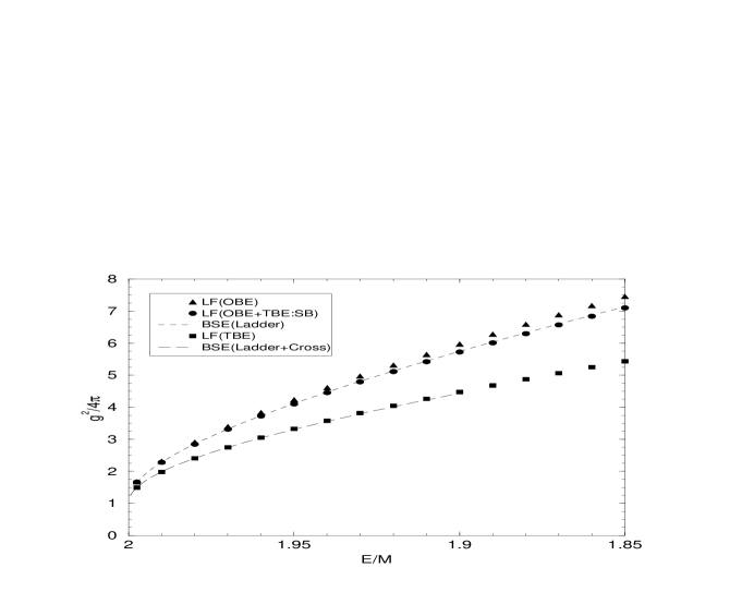
FIG. 4.: We display here three light-front calculations using the OBE, OBE+TBE:SB, and OBE+TBE potentials. The spectra for the Bethe-Salpeter equation for the ladder and ladder plus crossed kernels are also plotted. The curves for the ladder (ladder plus crossed) Bethe-Salpeter equation and the light-front OBE+TBE:SB (OBE+TBE) potentials are very close to each other, almost indistinguishable in this figure. $E$ is the energy of the ground state of two nucleons, and $M$ is the mass of the nucleons. The meson mass is $\mu=0.15M$. In terms of the binding energy $B$, $E=2M-B$.

If all one wanted was a way to approximate the spectra for Bethe-Salpeter equations with different kernels, one could just use the truncated potentials that the LFTOPT provide. However, the true goal is to approximate the spectra for the full ground state, which in this model is given by the FSR approach [25]. We expect that the non-perturbative potentials should give a better approximation of the full solution than the perturbative potentials, since the non-perturbative potentials attempt to incorporate physics from higher-order diagrams, although this is not immediately clear by looking at the forms of the potentials used. We plot the results for all of the light-front potentials described in this paper, the three truncated potentials (OBE, OBE+TBE:SB, and OBE+TBE) and the four non-perturbative potentials (symmetrized mass, retarded, instantaneous, and modified Green’s function) along with the results for the full theory in Fig. 5. For deeply-bound states, there is considerable disagreement between the perturbative results and the full results, while the non-perturbative results do better, with the modified-Green’s-function (MGF) potential achieving the closest agreement. For lightly-bound states, the results for all of the potentials appear converge to each other, close to the full result.

FIG. 5.: The spectra for the seven light-front potentials (OBE, OBE+TBE:SB, OBE+TBE, retarded, instantaneous, symmetrized mass, modified-Green’s-function) are plotted here along with the spectra for the full solution (FSR). The instantaneous curve lies very close to the symmetrized mass curve, hence the same line style is used for both.

For the modified-Green’s-function potential, only the first term of the expansion in $g^{2}$ was kept. In principle, higher-order terms could be calculated. However, since there was fairly good agreement between the OBE potential and the ladder Bethe-Salpeter equation, it is expected that the MGF potential will give results that are close to the ladder Bethe-Salpeter equation using the modified-Green’s-function.

VI Conclusions

In this paper, we consider the ground state of a massive Wick-Cutkosky model using a Hamiltonian derived from light-front dynamics. We examine three different truncations of the effective potential derived from the perturbative field theory, and four approximations that attempt to incorporate non-perturbative physics. For each of these potentials, we calculate the coupling constant that gives the ground-state for a given bound-state energy (the spectra), and compare to the spectra from different approaches found in the literature. We find fairly good agreement between all the methods for lightly-bound systems.

For the full range of binding energies studied, the results for calculations including one- and two-boson-exchange potentials agree with the Bethe-Salpeter equation using the physically equivalent truncation of the kernel within the numerical errors. (This is a consequence of examining the ground state. For the excited states more higher-order light-front time-ordered graphs are required to get the same level of agreement [7].) The agreement for the case with the stretched box diagrams (OBE+TBE:SB) has been shown previously by Sales et al. [23]; the result with the crossed-box contribution (OBE+TBE) is new. This excellent agreement with the Bethe-Salpeter results has an undesirable consequence: The BSE results are known to be a poor approximation of the full solution for deeply bound systems, so the truncated Hamiltonian approach cannot provide a good approximation to the full solution in that regime.

The non-perturbative potentials based on physical considerations give a better approximation of the full solution than the potentials obtained from LFTOPT. For all binding energies, the modified-Green’s-function potential achieves the closest agreement with the full solution of all the potentials considered here. However, there is still considerable disagreement between approximate potentials and the full result for deeply bound states. We interpret this as an indication that the approximations, while incorporating some non-perturbative physics, do not go far enough. In the weakly-bound regime, which is of relevance for deuteron calculations, the spectra for all of the potentials are close together, indicating that light-front dynamics provides a good description of lightly-bound systems.

A Notation, conventions, and useful relations

This is patterned after the review by Harindranath[4]. For a general four-vector $a$, we define the light-front variables

$$a^{\pm} = a^{0}\pm a^{3},$$ (A1)

$$\mathchoice{{\hbox{\boldmath$\displaystyle a$}}}{{\hbox{\boldmath$\textstyle a$}}}{{\hbox{\boldmath$\scriptstyle a$}}}{{\hbox{\boldmath$\scriptscriptstyle a$}}}_{\perp} = (a^{1},a^{2}),$$ (A2)

so the 4-vector $a^{\mu}$ can be denoted

$$a = (a^{+},a^{-},\mathchoice{{\hbox{\boldmath$\displaystyle a$}}}{{\hbox{\boldmath$\textstyle a$}}}{{\hbox{\boldmath$\scriptstyle a$}}}{{\hbox{\boldmath$\scriptscriptstyle a$}}}_{\perp}).$$ (A3)

Using this, we find that the scalar product is

$$a\cdot b = a^{\mu}b_{\mu}=\frac{1}{2}\left(a^{+}b^{-}+a^{-}b^{+}\right)-\mathchoice{{\hbox{\boldmath$\displaystyle a$}}}{{\hbox{\boldmath$\textstyle a$}}}{{\hbox{\boldmath$\scriptstyle a$}}}{{\hbox{\boldmath$\scriptscriptstyle a$}}}_{\perp}\cdot\mathchoice{{\hbox{\boldmath$\displaystyle b$}}}{{\hbox{\boldmath$\textstyle b$}}}{{\hbox{\boldmath$\scriptstyle b$}}}{{\hbox{\boldmath$\scriptscriptstyle b$}}}_{\perp}.$$ (A4)

This defines $g_{\mu\nu}$, with $g_{+-}=g_{-+}=1/2$, $g_{11}=g_{22}=-1$, and all other elements of $g$ vanish. The elements of $g^{\mu\nu}$ are obtained from the condition that $g^{\mu\nu}$ is the inverse of $g_{\mu\nu}$, so $g^{\alpha\beta}g_{\beta\lambda}=\delta^{\alpha}_{\lambda}$. Its elements are the same as those of $g_{\mu\nu}$, except for $g^{-+}=g^{+-}=2$. Thus,

$$a^{\pm} = 2a_{\mp}.$$ (A5)

and the partial derivatives are similarly given by

$$\partial^{\pm} = 2\partial_{\mp}=2\frac{\partial}{\partial x^{\mp}}.$$ (A6)

Moving to the physical consequences of this coordinate system, the commutation relations $[p^{\mu},x^{\nu}]=ig^{\mu\nu}$ yields

$$\,[p^{\pm},x^{\mp}] = 2i$$ (A7)

$$\,[\mathchoice{{\hbox{\boldmath$\displaystyle p$}}}{{\hbox{\boldmath$\textstyle p$}}}{{\hbox{\boldmath$\scriptstyle p$}}}{{\hbox{\boldmath$\scriptscriptstyle p$}}}_{\perp}^{i},\mathchoice{{\hbox{\boldmath$\displaystyle x$}}}{{\hbox{\boldmath$\textstyle x$}}}{{\hbox{\boldmath$\scriptstyle x$}}}{{\hbox{\boldmath$\scriptscriptstyle x$}}}_{\perp}^{j}] = -i\delta_{i,j},$$ (A8)

with the other commutators equal to zero. Thus, $\mathchoice{{\hbox{\boldmath$\displaystyle x$}}}{{\hbox{\boldmath$\textstyle x$}}}{{\hbox{\boldmath$\scriptstyle x$}}}{{\hbox{\boldmath$\scriptscriptstyle x$}}}_{\perp}^{i}$ is canonically conjugate to $\mathchoice{{\hbox{\boldmath$\displaystyle p$}}}{{\hbox{\boldmath$\textstyle p$}}}{{\hbox{\boldmath$\scriptstyle p$}}}{{\hbox{\boldmath$\scriptscriptstyle p$}}}_{\perp}^{i}$, and $x^{\pm}$ is conjugate to $p^{\mp}$. In light-front dynamics, $x^{+}$ plays the role of time (the light-front time), so $p^{-}$ is the light-front energy and the light-front Hamiltonian is given by $P^{-}$.

Particles have the light-front energy defined by the on-shell constraint $k^{2}=m^{2}$. This implies that the light-front energy is

$$k^{-} = \frac{m^{2}+\mathchoice{{\hbox{\boldmath$\displaystyle k$}}}{{\hbox{\boldmath$\textstyle k$}}}{{\hbox{\boldmath$\scriptstyle k$}}}{{\hbox{\boldmath$\scriptscriptstyle k$}}}_{\perp}^{2}}{k^{+}}.$$ (A9)

The free components of the momentum can be written as the light-front three-vector $\textstyle k$, denoted by

$$k = (k^{+},\mathchoice{{\hbox{\boldmath$\displaystyle k$}}}{{\hbox{\boldmath$\textstyle k$}}}{{\hbox{\boldmath$\scriptstyle k$}}}{{\hbox{\boldmath$\scriptscriptstyle k$}}}_{\perp}).$$ (A10)

B Conversion to matrix form

To solve for the bound-state wavefunction numerically, the light-front Schrödinger equation given in Eq. (44) must be discretized and cast in matrix form. The equation is first symmetrized to get

$$-\int_{0}^{\infty}dp_{\text{ET}}\int_{0}^{\pi/2}d\theta_{p}V_{S}^{+}(k_{\text{ET}},\theta_{k};p_{\text{ET}},\theta_{p})\psi_{S}^{\text{GS}}(p_{\text{ET}},\theta_{p}) = \psi_{S}^{\text{GS}}(k_{\text{ET}},\theta_{k}),$$ (B1)

where

$$V_{S}^{+}(k_{\text{ET}},\theta_{k};p_{\text{ET}},\theta_{p}) = B(k_{\text{ET}})A(k_{\text{ET}},\theta_{k})V^{+}(k_{\text{ET}},\theta_{k};p_{\text{ET}},\theta_{p})A(p_{\text{ET}},\theta_{p})B(p_{\text{ET}})$$ (B2)

$$\psi_{S}^{\text{GS}}(k_{\text{ET}},\theta_{k}) = B(k_{\text{ET}})^{-1}A(k_{\text{ET}},\theta_{k})\psi^{\text{GS}}(k_{\text{ET}},\theta_{k})$$ (B3)

$$A(k_{\text{ET}},\theta_{k}) = \sqrt{\frac{2k_{1}^{+}k_{2}^{+}k^{2}_{\text{ET}}\sin\theta_{k}}{(k^{0})}}$$ (B4)

$$B(k_{\text{ET}}) = \sqrt{\frac{-1}{E^{2}-4(k^{0})^{2}}}.$$ (B5)

Before discretizing the integrals, note that

$$\int_{0}^{\infty}dp\,f(p) = a\int_{0}^{1}du\left(f(au)+\frac{f(a/u)}{u^{2}}\right).$$ (B6)

Using this trick, the $p_{\text{ET}}$ integral in Eq. B1 can be written as an integral over a finite range. Since we are concerned with a bound state, the wavefunction is exponentially damped for large momenta, and the second term of Eq. (B6) converges as $u$ approaches zero.

All the integrals in Eq. B1 then are over a finite range, and can be discretized using Gauss-Legendre quadrature. The specific routines for the quadrature are given by Numerical Recipes in C [44]. This conversion gives a matrix equation that approximates the original Eq. B1,

$$-V_{S}^{+}(g(E),E)\psi_{S}^{\text{GS}} = \psi_{S}^{\text{GS}},$$ (B7)

where the explicit dependence of $V_{S}^{+}$ on the symmetrized potential on the binding energy $E$ and the coupling constant $g$ is shown. This equation must be solved self-consistently for the spectrum $g(E)$.

The approach we use is to first solve for the spectrum for the OBE potential. The eigenvalue equation

$$V_{S,\text{OBE}}^{+}(E)\psi_{S}^{\text{GS}} = \alpha\psi_{S}^{\text{GS}},$$ (B8)

where

$$\alpha = \frac{-1}{g_{\text{OBE}}(E)^{2}}.$$ (B9)

The ground-state wavefunction is the eigenvector that corresponds to the smallest eigenvalue $\alpha$. We calculate the wavefunction and the smallest coupling constant using EISPACK [45] routines for a range of energies to map out the spectrum.

Using the coupling constant for the OBE potential as a starting point, we can use Eq. B7 for higher-order potentials that include $N$ meson exchanges. For a given energy, the coupling constant $g(E)$ is initially chosen as $g_{\text{OBE}}(E)$, then we solve

$$\left[\sum_{n=1}^{N}g(E)^{2n}V_{S,(2n)}^{+}(E)\right]\psi_{S}^{\text{GS}} = \beta\psi_{S}^{\text{GS}},$$ (B10)

as an eigenvalue equation for $\beta$. The coupling constant $g(E)$ is varied until the the lowest eigenvalue is $\beta=-1$, at which point $g(E)$ is the correct value of the spectrum corresponding to the ground-state wavefunction $\psi_{S}^{\text{GS}}$.

C Azimuthal-angle integration of the OBE and MGF potentials

In this section, we evaluate the azimuthal-angle integration of the OBE potential in Eq. (54) and the first term in MGF potential in Eq. (141), using the prescription for azimuthal-angle integration given in Eq. (47). One of the integrals is easily done since since the potential is independent of the azimuthal angle between the two perpendicular momenta, so

$$V(k^{+},k_{\perp};p^{+},p_{\perp}) \propto \left[\theta(x-y)\int_{0}^{2\pi}\frac{d\phi}{A_{1}+B\cos\phi}+\theta(y-x)\int_{0}^{2\pi}\frac{d\phi}{A_{2}+B\cos\phi}\right],$$ (C1)

where

$$A_{1} = (k_{1}^{+}-p_{1}^{+})(E-p^{-}_{1}-k^{-}_{2})-\mu^{2}-p_{\perp}^{2}-k_{\perp}^{2}$$ (C2)

$$A_{2} = (p_{1}^{+}-k_{1}^{+})(E-k^{-}_{1}-p^{-}_{2})-\mu^{2}-p_{\perp}^{2}-k_{\perp}^{2}$$ (C3)

$$B = 2k_{\perp}p_{\perp}.$$ (C4)

The integrals in Eq. C1 are easily done to give, since the $A$’s are negative,

$$\int_{0}^{2\pi}\frac{d\phi}{A+B\cos\phi} = \frac{-2\pi}{\sqrt{A^{2}-B^{2}}}.$$ (C5)

Using this, the azimuthal-angle-averaged OBE potential is given by

$$V_{\text{OBE}}(k^{+},k_{\perp};p^{+},p_{\perp}) = -2\pi\left(\frac{M}{E}\right)^{2}E\left[\frac{\theta(x-y)}{\sqrt{A_{1}^{2}-B^{2}}}+\frac{\theta(y-x)}{\sqrt{A_{2}^{2}-B^{2}}}\right].$$ (C6)

It is straightforward to rewrite this equation for the potential in terms of the equal-time coordinates.

When the other terms in the MGF potential are azimuthal-angle averaged, integrations similar to the one given in Eq. C5 are encountered, with the denominator squared or cubed. We note that

$$\int_{0}^{2\pi}\frac{d\phi}{(A+B\cos\phi)^{2}} = \frac{-2\pi}{\sqrt{A^{2}-B^{2}}}\,\frac{A}{A^{2}-B^{2}}$$ (C7)

$$\int_{0}^{2\pi}\frac{d\phi}{(A+B\cos\phi)^{3}} = \frac{-2\pi}{\sqrt{A^{2}-B^{2}}}\,\frac{2A^{2}+B^{2}}{(A^{2}-B^{2})^{2}},$$ (C8)

so the azimuthal-angle-averaged MGF potential is given by

$$V_{\text{MGF}}(\mathchoice{{\hbox{\boldmath$\displaystyle k$}}}{{\hbox{\boldmath$\textstyle k$}}}{{\hbox{\boldmath$\scriptstyle k$}}}{{\hbox{\boldmath$\scriptscriptstyle k$}}}_{1},\mathchoice{{\hbox{\boldmath$\displaystyle p$}}}{{\hbox{\boldmath$\textstyle p$}}}{{\hbox{\boldmath$\scriptstyle p$}}}{{\hbox{\boldmath$\scriptscriptstyle p$}}}_{1};P) = -2\pi\left(\frac{M}{E}\right)^{2}\left[\frac{\theta(x-y)}{\sqrt{A_{1}^{2}-B^{2}}}\left(1+\frac{N_{p,21}+N_{k,12}}{2D_{1,2}}+\frac{N_{p,21}N_{k,12}}{2D_{1,3}}\right)\right.$$ (C10)

$$\phantom{-2\pi\left(\frac{M}{E}\right)^{2}\left[\right.}\left.+\frac{\theta(y-x)}{\sqrt{A_{2}^{2}-B^{2}}}\left(1+\frac{N_{k,21}+N_{p,12}}{2D_{2,2}}+\frac{N_{p,12}N_{k,21}}{2D_{2,3}}\right)\right],$$

where

$$D_{i,2} \equiv \frac{A^{2}-B^{2}}{A}$$ (C11)

$$D_{i,3} \equiv \frac{(A^{2}-B^{2})^{2}}{2A^{2}+B^{2}},$$ (C12)

and $i=1,2$.

D Azimuthal-Angle Integration and Loop integration of the TBE potentials

As in the previous section, we want the azimuthal-angle integrals of the TBE potentials given in Eqs. (65-87). For these potentials, there is also a loop integral that has to be done. We start by analyzing the equations schematically. Each of the terms in the TBE potentials can be written in the following form,

$$V_{\text{TBE}}(k^{+},k_{\perp};p^{+},p_{\perp}) = \int_{0}^{\infty}\frac{q_{\perp}dq_{\perp}}{2(2\pi)^{3}}\int_{0}^{1}dz\,J(k^{+},q^{+},p^{+})I(k^{+},k_{\perp},q^{+},q_{\perp},p^{+},p_{\perp})$$ (D1)

$$I(k^{+},k_{\perp},q^{+},q_{\perp},p^{+},p_{\perp}) = \int_{0}^{2\pi}d\phi_{q}d\phi_{p}\frac{1}{A_{1}+B_{1}\cos\phi_{q}}$$ (D4)

$$\times\frac{1}{A_{2}+B_{2}\cos\phi_{q}+C_{2}\cos\phi_{p}+D_{2}\cos(\phi_{p}-\phi_{q})}$$

$$\times\frac{1}{A_{3}+B_{3}\cos\phi_{q}+C_{3}\cos\phi_{p}+D_{3}\cos(\phi_{p}-\phi_{q})},$$

where the $A$’s, $B$’s, $C$’s, and $D$’s may have dependence on $k^{+}$, $k_{\perp}$, $p^{+}$, $p_{\perp}$, $q^{+}=zE$, and $q_{\perp}$; they are independent of the azimuthal angles. These functions can be easily determined for each potential by examining the forms of the original equations. The rotational invariance of the potential about the three-axis allows the $\phi_{k}$ integration to be done trivially.

In the integrand of $I$, only the last two terms depend on $\phi_{p}$. To emphasize this, we write

$$I(k^{+},k_{\perp},q^{+},q_{\perp},p^{+},p_{\perp}) = \int_{0}^{2\pi}d\phi_{q}\frac{I_{2}(k^{+},k_{\perp},\mathchoice{{\hbox{\boldmath$\displaystyle q$}}}{{\hbox{\boldmath$\textstyle q$}}}{{\hbox{\boldmath$\scriptstyle q$}}}{{\hbox{\boldmath$\scriptscriptstyle q$}}},p^{+},p_{\perp})}{(A_{1}+B_{1}\cos\phi_{q})(A_{2}+B_{2}\cos\phi_{q})(A_{3}+B_{3}\cos\phi_{q})}$$ (D5)

$$I_{2}(k^{+},k_{\perp},\mathchoice{{\hbox{\boldmath$\displaystyle q$}}}{{\hbox{\boldmath$\textstyle q$}}}{{\hbox{\boldmath$\scriptstyle q$}}}{{\hbox{\boldmath$\scriptscriptstyle q$}}},p^{+},p_{\perp}) = \int_{0}^{2\pi}\frac{d\phi_{p}}{(1+a_{2}\cos\phi_{p}+b_{2}\sin\phi_{p})(1+a_{3}\cos\phi_{p}+b_{3}\sin\phi_{p})}$$ (D6)

where, for $i=2,3$,

$$a_{i} = \frac{C_{i}+D_{i}\cos\phi_{q}}{A_{i}+B_{i}\cos\phi_{q}}$$ (D7)

$$b_{i} = \frac{D_{i}\sin\phi_{q}}{A_{i}+B_{i}\cos\phi_{q}}.$$ (D8)

The integral in $I_{2}$ is evaluated to obtain

$$I_{2}(k^{+},k_{\perp},\mathchoice{{\hbox{\boldmath$\displaystyle q$}}}{{\hbox{\boldmath$\textstyle q$}}}{{\hbox{\boldmath$\scriptstyle q$}}}{{\hbox{\boldmath$\scriptscriptstyle q$}}},p^{+},p_{\perp}) = \frac{2\pi}{(a_{2}-a_{3})^{2}+(b_{2}-b_{3})^{2}-(a_{2}b_{3}-a_{3}b_{2})^{2}}$$ (D10)

$$\times\left(\frac{a_{2}(a_{2}-a_{3})+b_{2}(b_{2}-b_{3})}{\sqrt{1-a_{2}^{2}-b_{2}^{2}}}+\frac{a_{3}(a_{3}-a_{2})+b_{3}(b_{3}-b_{2})}{\sqrt{1-a_{3}^{2}-b_{3}^{2}}}\right)$$

The remaining three-dimensional loop integral in $V_{\text{TBE}}$ on $\textstyle q$ is done using numeric techniques. The trick introduced in Appendix B to convert the semi-infinite $q_{\perp}$ integration into an integration on a compact range. Before doing the $z$ integral, the range of integration is limited by using the step functions. Gauss-Legendre quadrature, given by Numerical Recipes in C [44], is used to evaluate all the integrals.

Since each of the parts of the full TBE potential (TBE:SB, TBE:SX, …) should be hermitian and invariant under interchange of particle 1 and 2, these invariances can be used as a self-consistency check. Each matrix element is calculated twice, first by using the straightforward approach, then particle labels 1 and 2 are interchanged and it is calculated again. The results are compared, and if they differ by an unacceptable amount, the number of quadrature points is increased and the element is recalculated. In order to get the numerical accuracy of the potentials correct to within 1%, we start with ten points for the $q_{\perp}$ integral, six points for the $\phi_{q}$ integral, and three points for the $z$ integral, resulting in a three-dimensional integral using 180 points.

E Check of the Uncrossed Approximation

In this section, we want to check that how well the approximation

$$K_{\text{cross}} \approx K_{\text{ladder}}G_{C}K_{\text{ladder}},$$ (E1)

works. Since we are using a Hamiltonian theory and are interested in the potentials, we compare the potentials defined by

$$V_{\text{TBE:X}} = \frac{1}{E}g_{0}^{-1}\langle G_{0}K_{\text{cross}}G_{0}\rangle g_{0}^{-1}$$ (E2)

$$V_{\text{TBE:UX}} = \frac{1}{E}g_{0}^{-1}\langle G_{0}K_{\text{ladder}}G_{C}K_{\text{ladder}}G_{0}\rangle g_{0}^{-1}.$$ (E3)

The notation used here is defined in sections IV C and IV D.

The TBE crossed potential (TBE:X) can be written as

$$V_{\text{TBE:X}} = V_{\text{TBE:SX}}+V_{\text{TBE:TX}}+V_{\text{TBE:WX}}+V_{\text{TBE:ZX}},$$ (E4)

where the potentials on the right-hand side are defined in section III B. Calculation of the TBE approximate uncrossed potential (TBE:UX) is straightforward, but tedious. We find that

$$V_{\text{TBE:UX}}(E;\mathchoice{{\hbox{\boldmath$\displaystyle k$}}}{{\hbox{\boldmath$\textstyle k$}}}{{\hbox{\boldmath$\scriptstyle k$}}}{{\hbox{\boldmath$\scriptscriptstyle k$}}}_{1},\mathchoice{{\hbox{\boldmath$\displaystyle p$}}}{{\hbox{\boldmath$\textstyle p$}}}{{\hbox{\boldmath$\scriptstyle p$}}}{{\hbox{\boldmath$\scriptscriptstyle p$}}}_{1}) = \frac{1}{2}\Big{[}V_{\text{TBE:UX1}}(E;\mathchoice{{\hbox{\boldmath$\displaystyle k$}}}{{\hbox{\boldmath$\textstyle k$}}}{{\hbox{\boldmath$\scriptstyle k$}}}{{\hbox{\boldmath$\scriptscriptstyle k$}}}_{1},\mathchoice{{\hbox{\boldmath$\displaystyle p$}}}{{\hbox{\boldmath$\textstyle p$}}}{{\hbox{\boldmath$\scriptstyle p$}}}{{\hbox{\boldmath$\scriptscriptstyle p$}}}_{1})+V_{\text{TBE:UX1}}(E;\mathchoice{{\hbox{\boldmath$\displaystyle p$}}}{{\hbox{\boldmath$\textstyle p$}}}{{\hbox{\boldmath$\scriptstyle p$}}}{{\hbox{\boldmath$\scriptscriptstyle p$}}}_{1},\mathchoice{{\hbox{\boldmath$\displaystyle k$}}}{{\hbox{\boldmath$\textstyle k$}}}{{\hbox{\boldmath$\scriptstyle k$}}}{{\hbox{\boldmath$\scriptscriptstyle k$}}}_{1})$$ (E6)

$$\phantom{\frac{1}{2}\Big{[}}+V_{\text{TBE:UX2}}(E;\mathchoice{{\hbox{\boldmath$\displaystyle k$}}}{{\hbox{\boldmath$\textstyle k$}}}{{\hbox{\boldmath$\scriptstyle k$}}}{{\hbox{\boldmath$\scriptscriptstyle k$}}}_{1},\mathchoice{{\hbox{\boldmath$\displaystyle p$}}}{{\hbox{\boldmath$\textstyle p$}}}{{\hbox{\boldmath$\scriptstyle p$}}}{{\hbox{\boldmath$\scriptscriptstyle p$}}}_{1})+V_{\text{TBE:UX2}}(E;\mathchoice{{\hbox{\boldmath$\displaystyle p$}}}{{\hbox{\boldmath$\textstyle p$}}}{{\hbox{\boldmath$\scriptstyle p$}}}{{\hbox{\boldmath$\scriptscriptstyle p$}}}_{1},\mathchoice{{\hbox{\boldmath$\displaystyle k$}}}{{\hbox{\boldmath$\textstyle k$}}}{{\hbox{\boldmath$\scriptstyle k$}}}{{\hbox{\boldmath$\scriptscriptstyle k$}}}_{1})\Big{]},$$

where

$$V_{\text{TBE:UX1}}(E;\mathchoice{{\hbox{\boldmath$\displaystyle k$}}}{{\hbox{\boldmath$\textstyle k$}}}{{\hbox{\boldmath$\scriptstyle k$}}}{{\hbox{\boldmath$\scriptscriptstyle k$}}}_{1},\mathchoice{{\hbox{\boldmath$\displaystyle p$}}}{{\hbox{\boldmath$\textstyle p$}}}{{\hbox{\boldmath$\scriptstyle p$}}}{{\hbox{\boldmath$\scriptscriptstyle p$}}}_{1}) = \left(\frac{M}{E}\right)^{4}\int\frac{d^{2}q_{\perp}}{2(2\pi)^{3}}\left[\int_{0}^{1}dz\frac{\theta(x-z)\theta(z-y)}{(x-z)z^{2}(z-y)}\right.$$ (E10)

$$\phantom{\left(\frac{M}{E}\right)^{4}\int\frac{d^{2}q_{\perp}}{2(2\pi)^{3}}\left[\right.}\left.\times\frac{1}{E-p_{1}^{-}-k_{2}^{-}-\omega^{-}(\mathchoice{{\hbox{\boldmath$\displaystyle q$}}}{{\hbox{\boldmath$\textstyle q$}}}{{\hbox{\boldmath$\scriptstyle q$}}}{{\hbox{\boldmath$\scriptscriptstyle q$}}}_{1}-\mathchoice{{\hbox{\boldmath$\displaystyle p$}}}{{\hbox{\boldmath$\textstyle p$}}}{{\hbox{\boldmath$\scriptstyle p$}}}{{\hbox{\boldmath$\scriptscriptstyle p$}}}_{1})-\omega^{-}(\mathchoice{{\hbox{\boldmath$\displaystyle k$}}}{{\hbox{\boldmath$\textstyle k$}}}{{\hbox{\boldmath$\scriptstyle k$}}}{{\hbox{\boldmath$\scriptscriptstyle k$}}}_{1}-\mathchoice{{\hbox{\boldmath$\displaystyle q$}}}{{\hbox{\boldmath$\textstyle q$}}}{{\hbox{\boldmath$\scriptstyle q$}}}{{\hbox{\boldmath$\scriptscriptstyle q$}}}_{1})}\right.$$

$$\phantom{\left(\frac{M}{E}\right)^{4}\int\frac{d^{2}q_{\perp}}{2(2\pi)^{3}}\left[\right.}\left.\times\left(\frac{1}{E-q_{1}^{-}-k_{2}^{-}-\omega^{-}(\mathchoice{{\hbox{\boldmath$\displaystyle k$}}}{{\hbox{\boldmath$\textstyle k$}}}{{\hbox{\boldmath$\scriptstyle k$}}}{{\hbox{\boldmath$\scriptscriptstyle k$}}}_{1}-\mathchoice{{\hbox{\boldmath$\displaystyle q$}}}{{\hbox{\boldmath$\textstyle q$}}}{{\hbox{\boldmath$\scriptstyle q$}}}{{\hbox{\boldmath$\scriptscriptstyle q$}}}_{1})}\right)^{2}\right]$$

$$\phantom{\left(\frac{M}{E}\right)^{4}\int\frac{d^{2}q_{\perp}}{2(2\pi)^{3}}}+\{1\leftrightarrow 2\}$$

$$V_{\text{TBE:UX2}}(E;\mathchoice{{\hbox{\boldmath$\displaystyle k$}}}{{\hbox{\boldmath$\textstyle k$}}}{{\hbox{\boldmath$\scriptstyle k$}}}{{\hbox{\boldmath$\scriptscriptstyle k$}}}_{1},\mathchoice{{\hbox{\boldmath$\displaystyle p$}}}{{\hbox{\boldmath$\textstyle p$}}}{{\hbox{\boldmath$\scriptstyle p$}}}{{\hbox{\boldmath$\scriptscriptstyle p$}}}_{1}) = \left(\frac{M}{E}\right)^{4}\int\frac{d^{2}q_{\perp}}{2(2\pi)^{3}}\left[\int_{0}^{1}dz\frac{\theta(x-z)\theta(y-z)}{(x-z)z^{2}(y-z)}\right.$$ (E14)

$$\phantom{\left(\frac{M}{E}\right)^{4}\int\frac{d^{2}q_{\perp}}{2(2\pi)^{3}}\left[\right.}\left.\times\frac{1}{E-q_{1}^{-}-p_{2}^{-}-\omega^{-}(\mathchoice{{\hbox{\boldmath$\displaystyle p$}}}{{\hbox{\boldmath$\textstyle p$}}}{{\hbox{\boldmath$\scriptstyle p$}}}{{\hbox{\boldmath$\scriptscriptstyle p$}}}_{1}-\mathchoice{{\hbox{\boldmath$\displaystyle q$}}}{{\hbox{\boldmath$\textstyle q$}}}{{\hbox{\boldmath$\scriptstyle q$}}}{{\hbox{\boldmath$\scriptscriptstyle q$}}}_{1})}\right.$$

$$\phantom{\left(\frac{M}{E}\right)^{4}\int\frac{d^{2}q_{\perp}}{2(2\pi)^{3}}\left[\right.}\left.\times\left(\frac{1}{E-q_{1}^{-}-k_{2}^{-}-\omega^{-}(\mathchoice{{\hbox{\boldmath$\displaystyle k$}}}{{\hbox{\boldmath$\textstyle k$}}}{{\hbox{\boldmath$\scriptstyle k$}}}{{\hbox{\boldmath$\scriptscriptstyle k$}}}_{1}-\mathchoice{{\hbox{\boldmath$\displaystyle q$}}}{{\hbox{\boldmath$\textstyle q$}}}{{\hbox{\boldmath$\scriptstyle q$}}}{{\hbox{\boldmath$\scriptscriptstyle q$}}}_{1})}\right)^{2}\right]$$

$$\phantom{\left(\frac{M}{E}\right)^{4}\int\frac{d^{2}q_{\perp}}{2(2\pi)^{3}}}+\{1\leftrightarrow 2\}.$$

Now consider the azimuthal-angle and loop integrals for these potentials. The approach used is similar to that of section D. Analyzing the potentials reveals that each of the terms can be written in the following schematic form,

$$V_{\text{TBE:UX,i}}(k^{+},k_{\perp};p^{+},p_{\perp}) = \int_{0}^{\infty}\frac{q_{\perp}dq_{\perp}}{2(2\pi)^{3}}\int_{0}^{1}dz\,J(k^{+},q^{+},p^{+})I_{i}(k^{+},k_{\perp},q^{+},q_{\perp},p^{+},p_{\perp})$$ (E15)

$$I_{i}(k^{+},k_{\perp},q^{+},q_{\perp},p^{+},p_{\perp}) = \int_{0}^{2\pi}\frac{d\phi_{q}d\phi}{A_{1,i}+B_{1,i}\cos\phi_{q}+C_{1,i}\cos\phi}\left(\frac{1}{A_{2}+B_{2}\cos\phi_{q}}\right)^{2},$$ (E16)

where $\phi=-\phi_{q}+\phi_{p}$, and the $A$’s, $B$’s, and $C$’s may have dependence on $k^{+}$, $k_{\perp}$, $p^{+}$, $p_{\perp}$, $q^{+}=zE$, and $q_{\perp}$; they are independent of the azimuthal angles. These factors can be easily determined for each potential by examining the forms of the original equations. The rotational invariance of the potential about the three-axis allows the $\phi_{k}$ integration to be done trivially. The $\phi$ integral is easily done to obtain

$$I(k^{+},k_{\perp},q^{+},q_{\perp},p^{+},p_{\perp}) = -2\pi\int_{0}^{2\pi}d\phi_{q}\frac{1}{\sqrt{a_{i}^{2}-C_{1,i}^{2}}}\left(\frac{1}{A_{2}+B_{2}\cos\phi_{q}}\right)^{2},$$ (E17)

where

$$a_{i} = A_{1,i}+B_{1,i}\cos\phi_{q}.$$ (E18)

Further simplification is possible for $V_{\text{TBE:UX2}}$, since for that potential $B_{1,2}=0$,

$$I(k^{+},k_{\perp},q^{+},q_{\perp},p^{+},p_{\perp}) = \frac{(2\pi)^{2}A_{2}}{\sqrt{A_{1,2}^{2}-C_{1,2}^{2}}\sqrt{A_{2}^{2}-B_{2}^{2}}(A_{2}^{2}-B_{2}^{2})}.$$ (E19)

The techniques discussed in the previous section are used to do the remaining loop integrals.

The spectra for the OBE+TBE:SB+TBE:UX potential can be calculated and compared to the OBE+TBE:SB+TBE:X potential (which is the same as the OBE+TBE potential), the modified-Green’s-function potential, and the ladder plus crossed Bethe-Salpeter equation. The spectra are plotted in Fig. 6. The spectra for the TBE:UX, TBE:X and BSE all lie close to each other, which shows that that the uncrossed approximation is valid.

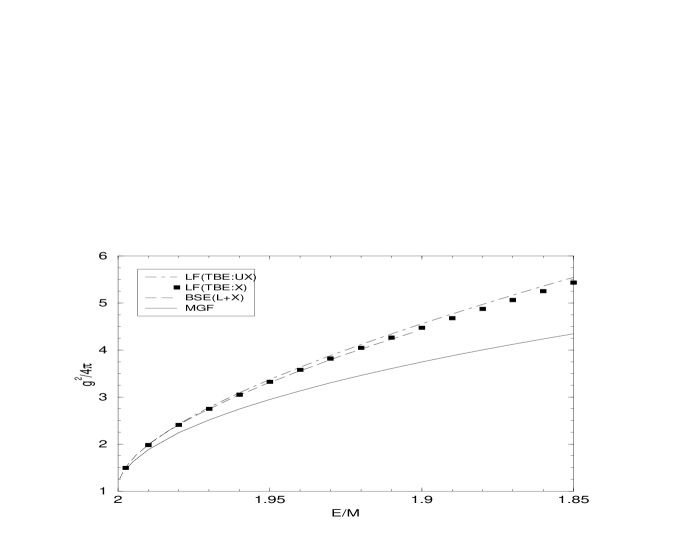
FIG. 6.: The spectra are plotted for the potential derived from the TBE truncation of the uncrossed approximation (OBE+TBE:SB+TBE:UX, denoted in the figure by TBE:UX), the TBE potential (OBE+TBE, denoted by TBE:X), the ladder plus crossed Bethe-Salpeter equation (BSE(L+X)), and the modified-Green’s-function potential (MGF). Except for the MGF spectrum, all the curves lie close to each other.

This shows that the important approximation in the modified-Green’s-function approach is not the uncrossed approximation, but the addition of the extra interaction terms in Eq. (118) which serve to mimic the higher order interactions.

REFERENCES

- [1] L. C. Alexa et al. [Jefferson Lab Hall A Collaboration], Phys. Rev. Lett. 82, 1374 (1999) [nucl-ex/9812002].
- [2] P. A. Dirac, Rev. Mod. Phys. 21, 392 (1949).
- [3] S. J. Brodsky, H. Pauli and S. S. Pinsky, Phys. Rept. 301, 299 (1998) [hep-ph/9705477].
- [4] A. Harindranath, hep-ph/9612244.
- [5] T. Heinzl, hep-th/9812190.
- [6] G. A. Miller, Phys. Rev. C56, 2789 (1997) [nucl-th/9706028].
- [7] J. R. Cooke, G. A. Miller and D. R. Phillips, nucl-th/9910013.
- [8] Y. A. Simonov and J. A. Tjon, Annals Phys. 228, 1 (1993).
- [9] Y. Nambu, Prog. Theor. Phys. 5, 614 (1950).
- [10] J. Schwinger, Proc. Nat. Acad. Sci. 37, 452 (1951); 37, 455 (1951).
- [11] M. Gell-Mann and F. Low, Phys. Rev. 84, 350 (1951).
- [12] E. E. Salpeter and H. A. Bethe, Phys. Rev. 84, 1232 (1951).
- [13] F. Gross, Phys. Rev. C26, 2203 (1982).
- [14] M.J. Levine, J.A. Tjon, and J. Wright, Phys. Rev. Lett. 16, 962 (1966),
- [15] M.J. Levine, J. Wright, and J.A. Tjon, Phys. Rev. 154, 1433 (1967).
- [16] M.J. Levine and J. Wright, Phys. Rev. D2, 2509 (1970).
- [17] J. Carbonell, B. Desplanques, V. A. Karmanov and J. F. Mathiot, Phys. Rept. 300, 215 (1998) [nucl-th/9804029].
- [18] N. C. Schoonderwoerd, B. L. Bakker and V. A. Karmanov, Phys. Rev. C58, 3093 (1998) [hep-ph/9806365].
- [19] G. Baym, Phys. Rev. 117, 886 (1960).
- [20] J. J. Wivoda and J. R. Hiller, Phys. Rev. D47, 4647 (1993).
- [21] C. Savkli, J. Tjon and F. Gross, Phys. Rev. C60, 055210 (1999) [hep-ph/9906211].
- [22] R. Rosenfelder and A. W. Schreiber, Phys. Rev. D53, 3337 (1996) [nucl-th/9504002]; 53, 3354 (1996) [nucl-th/9504005].
- [23] J. H. Sales, T. Frederico, B. V. Carlson and P. U. Sauer, nucl-th/9909029.
- [24] N. E. Ligterink and B. L. Bakker, Phys. Rev. D52, 5954 (1995) [hep-ph/9412315].
- [25] T. Nieuwenhuis and J. A. Tjon, Phys. Rev. Lett. 77, 814 (1996) [hep-ph/9606403].
- [26] G. C. Wick, Phys. Rev. 96, 1124 (1954); R. E. Cutkosky, ibid. 96, 1135 (1954).
- [27] M. V. Terentev, Sov. J. Nucl. Phys. 24, 106 (1976).
- [28] A. Klein, Phys. Rev. 90, 1101 (1953).
- [29] D. R. Phillips and S. J. Wallace, Phys. Rev. C54, 507 (1996) [nucl-th/9603008].
- [30] A. D. Lahiff and I. R. Afnan, Phys. Rev. C56, 2387 (1997) [nucl-th/9708037].
- [31] S. Chang and S. Ma, Phys. Rev. 180, 1506 (1969).
- [32] M. Krautgartner, H. C. Pauli and F. Wolz, Phys. Rev. D45, 3755 (1992).
- [33] U. Trittmann and H. Pauli, hep-th/9705021.
- [34] J. A. Eden and M. F. Gari, Phys. Rev. C53, 1510 (1996) [nucl-th/9601025], S. Okubo, Prog. Theor. Phys. 12, 603 (1954).
- [35] R. Blankenbecler and R. Sugar, Phys. Rev. 142, 1051 (1966).
- [36] F. Gross, Phys. Rev. 186, 1448 (1969).
- [37] S. J. Wallace, in Nuclear and Particle Physics on the Light Cone (LAMPF Workshop), 1988, edited by M.B. Johnson and L.S. Kisslinger (World Scientific, Singapore, 1989), p. 477.
- [38] S. J. Wallace and V. B. Mandelzweig, Nucl. Phys. A503, 673 (1989).
- [39] R.M. Woloshyn and A.D. Jackson, Nucl. Phys. B64, 269 (1973).
- [40] D. R. Phillips and I. R. Afnan, Phys. Rev. C54, 1542 (1996) [nucl-th/9605004].
- [41] C. Schwartz, Phys. Rev. 137, B717 (1965).
- [42] L. Theussl and B. Desplanques, nucl-th/9908007.
- [43] D.R. Phillips (private communication).
- [44] W.H. Press, S.A. Teukolsky, W.T. Vetterling, and B.P. Flannery, Numerical Recipes in C, second edition (Cambridge University Press, New York, 1992), p. 147.
- [45] B.T. Smith et al, Matrix Eigensystem Routines – EISPACK Guide, Lecture Notes in Computer Science, Vol. 6, Second Edition, Springer-Verlag, New York, Heidelberg, Berlin, 1976; B.S. Garbow et al, Matrix Eigensystem Routines – EISPACK Guide Extension, Lecture Notes in Computer Science, Vol. 51, Springer-Verlag, New York, Heidelberg, Berlin, 1977.