The $F/D$ ratio and meson-baryon couplings from QCD sum rules-II

Abstract

Using QCD sum rules, we compute the diagonal meson-baryon couplings, $\pi NN$, $\eta NN$, $\pi\Xi\Xi$, $\eta\Xi\Xi$, $\pi\Sigma\Sigma$ and $\eta\Sigma\Sigma$, from the baryon-baryon correlation function with a meson, $i\int d^{4}x~{}e^{iq\cdot x}\langle 0|TJ_{B}(x){\bar{J}}_{B}(0)|M(p)\rangle$. The calculations are performed to leading order in $p_{\mu}$ by considering the two separate Dirac structures, $i\gamma_{5}\gamma_{\mu}p^{\mu}$ and $\gamma_{5}\sigma_{\mu\nu}{q^{\mu}p^{\nu}}$ separately. We first improve the previous sum rule calculations on these Dirac structures for the $\pi NN$ coupling by including three-particle pion wave functions of twist 4 and then extend the formalism to calculate the other couplings, $\eta NN$, $\pi\Xi\Xi$, $\eta\Xi\Xi$, $\pi\Sigma\Sigma$ and $\eta\Sigma\Sigma$. In the SU(3) symmetric limit, we identify the terms responsible for the $F/D$ ratio in the OPE by matching the obtained couplings with their SU(3) relations. Depending on the Dirac structure considered, we find different identifications for the $F/D$ ratio. The couplings including the SU(3) breaking effects are also discussed within our approach.

I INTRODUCTION

The QCD sum rule [1] is often used to determine hadronic parameters from QCD. In this framework, an interpolating field appropriate for the hadron of concern is introduced using quark and gluon fields and used to construct an appropriate correlation function. The correlation function is calculated on the one hand by the operator product expansion (OPE) at the deep Euclidean region of the correlator momentum $q^{2}\rightarrow-\infty$ using QCD degrees of freedom. On the other hand, its phenomenological form is constructed using hadronic degrees of freedom. In most cases of practical QCD sum rule calculations, the phenomenological form is analytic in the complex $q^{2}$ plane except along the positive real axis. Through a dispersion relation, the nonanalytic structure along the positive real axis is matched to the QCD representation of the correlator at $q^{2}\rightarrow-\infty$ and the hadron parameter of concern is extracted in terms of QCD parameters.

The QCD sum rule framework has been widely used to calculate various hadronic properties [2]. Among various applications, determining meson-baryon couplings is of particular interest because meson-baryon couplings are important ingredients for analyzing baryon-baryon interactions. Their values determined from QCD may provide important constraints in constructing baryon-baryon potentials [3]. One main feature of meson-baryon couplings is SU(3) symmetry as it provides a systematic classification of the couplings [4] in terms of the two parameters, the $\pi NN$ coupling and the $F/D$ ratio. This systematic classification of the couplings is a basis for making realistic potential models for hyperon-baryon interactions [5, 6]. In this approach, however, implementing the SU(3) breaking in the couplings is somewhat limited because the models used rely solely on hadronic degrees of freedom and thus the way of introducing the SU(3) breaking terms in the model may not be unique. Moreover, the baryon-baryon scattering data used in the fitting processes are not precise enough to pick out a specific mesonic channel. Therefore, it would be useful to constrain each model of meson-baryon coupling directly from other non-perturbative methods of QCD, such as QCD sum rules.

Recently, the two-point correlation function of the nucleon interpolating fields with an external pion field

$$\Pi(q,p)=i\int d^{4}xe^{iq\cdot x}\langle 0|T[J_{N}(x){\bar{J}}_{N}(0)]|\pi(p)\rangle\ .$$ (1)

has been extensively used to calculate the pion-nucleon coupling within the conventional QCD sum rule method [7, 8, 9, 10, 11, 12]. Another approach relying on the three-point function [13] gives results that may contain non-negligible contributions from the higher resonances $\pi(1300)$ and $\pi(1800)$ [14]. Moreover, using the two-point correlation function, the sum rule can be easily extended to other meson-baryon couplings and the SU(3) limit can be easily taken to identify the $F/D$ ratio. Among various developments using Eq. (1), one interesting attempt is to calculate the coupling beyond the chiral limit [9] by considering the Dirac structure $i\gamma_{5}$ at the order $p^{2}=m_{\pi}^{2}$. As a consistent chiral counting, linear terms in the quark mass $m_{q}$ have been included in the OPE side. The pion-nucleon coupling obtained by combining this sum rule with the nucleon chiral-odd sum rule seems to be quite satisfactory.

This sum rule beyond the chiral limit has been recently applied to other meson-baryon couplings such as $\eta NN$, $\pi\Xi\Xi$, $\eta\Xi\Xi$, $\pi\Sigma\Sigma$ and $\eta\Sigma\Sigma$ [10]. The OPE of each sum rule is found to satisfy the SU(3) relations for the couplings proposed in Ref. [4], which enables us to identify the terms responsible for the $F/D$ ratio. This nontrivial observation for the $F/D$ ratio, which is a natural consequence of using the SU(3) symmetric interpolating fields, was possible because the sum rules are constructed beyond the chiral limit. The sum rules, if constructed in the soft-meson limit for example, provide the OPE trivially satisfying the SU(3) relations with $F/D=0$. Therefore, going beyond the chiral limit especially in the $i\gamma_{5}$ sum rules is important for obtaining nontrivial value of the $F/D$ ratio. From this sum rule, the ratio obtained is $F/D\sim 0.2$ substantially smaller than what it has been known from SU(6) consideration. Furthermore, meson-baryon couplings after taking into account the SU(3) breaking in the OPE as well as in the phenomenological part undergo huge changes from their SU(3) symmetric values. This finding is not consistent with Nijmegen potentials [5, 6] or with common assumptions in studying hypernuclei.

On the other hand, similar sum rule calculations can be performed for the couplings using Dirac structures other than the $i\gamma_{5}$ structure. As discussed in Ref. [8], the correlation function Eq. (1) contains the other Dirac structures, $i\gamma_{5}{\hat{p}}$ (${\hat{p}}\equiv\gamma_{\mu}p^{\mu}$ ) and $\gamma_{5}\sigma_{\mu\nu}q^{\mu}p^{\nu}$, which can also be used to construct sum rules for the $\pi NN$ coupling beyond the soft-pion limit. Of course, it is straightforward to extend the $i\gamma_{5}{\hat{p}}$ and $\gamma_{5}\sigma_{\mu\nu}q^{\mu}p^{\nu}$ sum rules and calculate the couplings $\eta NN$, $\pi\Xi\Xi$, $\eta\Xi\Xi$, $\pi\Sigma\Sigma$and $\eta\Sigma\Sigma$. In the SU(3) limit, the OPE should satisfy the SU(3) relations for the couplings, which will allow us to identify the OPE terms responsible for the $F/D$ ratio. This is our primary purpose of this work. In particular, we will see if the identifications made from these Dirac structures are consistent with the previous identification made in Ref. [10], or if the Dirac structure dependence of the sum rule results [8] still persists in these identifications. Once the sum rules are constructed, it will be straightforward to introduce the SU(3) breaking within this framework and see how the SU(3) breaking affects the couplings.

As presented in Ref. [7], the $\gamma_{5}\sigma_{\mu\nu}q^{\mu}p^{\nu}$ Dirac structure has nice features in calculating the $\pi NN$ coupling. To be specific, this sum rule provides a coupling independent of the models employed to construct its phenomenological side and the result is rather stable against the variation of the continuum parameter. Indeed, this structure has been further applied to the study of the couplings $g_{NK\Lambda}$ and $g_{NK\Sigma}$ [15] and other pion-baryon couplings [16]. Even though the calculated $\pi NN$ coupling is a bit smaller than the empirical value, it may be useful to investigate this sum rule further and improve the previous result. In this work, we will revisit the previous $\pi NN$ calculations and improve the OPE calculation in the highest dimensions. We then apply the framework to other meson-baryon couplings in the SU(3) sector to identify the OPE responsible for the $F/D$ ratio.

The other Dirac structure $i\gamma_{5}{\hat{p}}$, as discussed in Ref. [8], is found not to be reliable for calculating the $\pi NN$ coupling as it contains large contributions from the continuum. The extracted value is highly sensitive to the continuum threshold. Nevertheless, we will study this sum rule again for the completeness first of all. We will improve the OPE calculation by including higher dimensional operators. Then, by extending the sum rule to the other couplings, we will see how the identification for the $F/D$ ratio from this Dirac structure is different from the ones obtained from other Dirac structures.

The paper is organized as follows. In Section II, we will revisit the $i\gamma_{5}{\hat{p}}$ and $\gamma_{5}\sigma_{\mu\nu}q^{\mu}p^{\nu}$ sum rules for $\pi NN$ and refine the OPE calculation. We then extend this framework to construct $\eta NN$ sum rules in Section III and identify the OPE responsible for the $F/D$ ratio. In Section IV, we construct sum rules for the couplings, $\pi\Xi\Xi$, $\eta\Xi\Xi$, $\pi\Sigma\Sigma$ and $\eta\Sigma\Sigma$. We confirm that the OPE of each sum rule satisfies the SU(3) relations with the identification of the $F/D$ ratio made in Section III. In Section V, we present our analysis in the SU(3) symmetric limit. The analysis beyond the SU(3) limit is given in Section VI but only for the $\gamma_{5}\sigma_{\mu\nu}q^{\mu}p^{\nu}$ sum rules.

II Pion-nucleon coupling determined beyond the soft-pion limit

In this section, we construct QCD sum rules for the $\pi^{0}pp$ coupling at the first order of the pion momentum ${\cal O}(p_{\mu})$, to predict the coupling beyond the soft-pion limit. To do this, we use the two-point correlation function with a pion,

$$\Pi(q,p)=i\int d^{4}xe^{iq\cdot x}\langle 0|T[J_{p}(x){\bar{J}}_{p}(0)]|\pi^{0}(p)\rangle\ \equiv\int d^{4}xe^{iq\cdot x}\Pi(x,p)\ .$$ (2)

Here $J_{p}$ is the proton interpolating field suggested by Ioffe [17],

$$J_{p}=\epsilon_{abc}[u_{a}^{T}C\gamma_{\mu}u_{b}]\gamma_{5}\gamma^{\mu}d_{c}\ ,$$ (3)

where $a,b,c$ are color indices, $T$ denotes the transpose with respect to the Dirac indices, $C$ the charge conjugation. Using this correlator, we construct the sum rules beyond the soft-pion limit by considering the Dirac structures, $i\gamma_{5}{\hat{p}}$ (${\hat{p}}\equiv\gamma_{\mu}p^{\mu}$) and $\gamma_{5}\sigma_{\mu\nu}q^{\mu}p^{\nu}$. After taking out the Dirac structures containing one power of the pion momentum, we take the limit $p_{\mu}\rightarrow 0$ in the rest of the correlator. These sum rules have been considered in Ref. [7, 8] but we revisit them here to improve the OPE calculations. By considering the sum rules for $\pi^{0}pp$ instead of $\pi^{+}pn$, we can easily extend the formalism to the other diagonal meson-baryon couplings, $\eta NN$, $\pi\Xi\Xi$, $\eta\Sigma\Sigma$ and so on.

The QCD side of the correlator Eq.(2) is calculated via the operator product expansion (OPE) at the deep spacelike region $q^{2}\rightarrow-\infty$. In our calculations, we use the vacuum saturation hypothesis to factor out quark-antiquark component with a pion (denoted by $D^{q}_{ab}$ below) from the correlator. The rest of the correlator is basically time-ordered products of quark fields which are normally evaluated by background-field techniques [18]. Accordingly, it is straightforward to write the correlator in the coordinate space,

$$\Pi(x,p)=-i\epsilon_{abc}\epsilon_{a^{\prime}b^{\prime}c^{\prime}}\Bigg{\{} \gamma_{5}\gamma^{\mu}D^{d}_{cc^{\prime}}\gamma^{\nu}\gamma_{5}{\rm Tr}\left[iS_{aa^{\prime}}(x)(\gamma_{\nu}C)^{T}iS_{bb^{\prime}}^{T}(x)(C\gamma_{\mu})^{T}\right]$$ (4)

$$- \gamma_{5}\gamma^{\mu}D^{d}_{cc^{\prime}}\gamma^{\nu}\gamma_{5}{\rm Tr}\left[iS_{ab^{\prime}}(x)\gamma_{\nu}CiS_{ba^{\prime}}^{T}(x)(C\gamma_{\mu})^{T}\right]$$ (5)

$$- \gamma_{5}\gamma^{\mu}iS_{cc^{\prime}}(x)\gamma^{\nu}\gamma_{5}{\rm Tr}\left[iS_{ab^{\prime}}(x)\gamma_{\nu}C(D^{u}_{ba^{\prime}})^{T}(C\gamma_{\mu})^{T}\right]$$ (6)

$$+ \gamma_{5}\gamma^{\mu}iS_{cc^{\prime}}(x)\gamma^{\nu}\gamma_{5}{\rm Tr}\left[iS_{aa^{\prime}}(x)(\gamma_{\nu}C)^{T}(D^{u}_{bb^{\prime}})^{T}(C\gamma_{\mu})^{T}\right]$$ (7)

$$+ \gamma_{5}\gamma^{\mu}iS_{cc^{\prime}}(x)\gamma^{\nu}\gamma_{5}{\rm Tr}\left[D^{u}_{aa^{\prime}}(\gamma_{\nu}C)^{T}iS_{bb^{\prime}}^{T}(x)(C\gamma_{\mu})^{T}\right]$$ (8)

$$- \gamma_{5}\gamma^{\mu}iS_{cc^{\prime}}(x)\gamma^{\nu}\gamma_{5}{\rm Tr}\left[D^{u}_{ab^{\prime}}\gamma_{\nu}CiS_{ba^{\prime}}^{T}(x)(C\gamma_{\mu})^{T}\right]\Bigg{\}}\ .$$ (9)

The quark propagators $iS(x)$ inside the traces are the u-quark propagators and the ones outside of the traces are the d-quark propagators. For the time being, we postpone discussions on the gluonic contributions which are obtained by moving a gluon tensor from a quark propagator into the quark-antiquark component with a pion (constituting thus the three-particle pion wave functions according to the nomenclature commonly used in the light-cone QCD sum rules [20]). Then, it is possible to write the quark-antiquark component with a pion in terms of three matrix elements involving a pion. Namely, for $q={u~{}{\rm or}~{}d}$-quark, we have

$$(D_{aa^{\prime}}^{q})^{\alpha\beta} \equiv \langle 0|q^{\alpha}_{a}(x){\bar{q}}^{\beta}_{a^{\prime}}(0)|\pi^{0}(p)\rangle\$$ (10)

$$= {\delta_{aa^{\prime}}\over 12}(\gamma^{\mu}\gamma_{5})^{\alpha\beta}\langle 0|{\bar{q}}(0)\gamma_{\mu}\gamma_{5}q(x)|\pi^{0}(p)\rangle\ +{\delta_{aa^{\prime}}\over 12}(i\gamma_{5})^{\alpha\beta}\langle 0|{\bar{q}}(0)i\gamma_{5}q(x)|\pi^{0}(p)\rangle$$ (12)

$$-{\delta_{aa^{\prime}}\over 24}(\gamma_{5}\sigma^{\mu\nu})^{\alpha\beta}\langle 0|{\bar{q}}(0)\gamma_{5}\sigma_{\mu\nu}q(x)|\pi^{0}(p)\rangle\ .$$

The pseudoscalar pion matrix element $\langle 0|{\bar{q}}(0)i\gamma_{5}q(x)|\pi^{0}(p)\rangle$ contributes only to the $i\gamma_{5}$ structure of the correlator, not participating in the sum rules of the Dirac structures $i\gamma_{5}{\hat{p}}$ and $\gamma_{5}\sigma_{\mu\nu}q^{\mu}p^{\nu}$. The rest two components differ by their chirality and both contribute to the $i\gamma_{5}{\hat{p}}$ and $\gamma_{5}\sigma_{\mu\nu}q^{\mu}p^{\nu}$ sum rules.

At the first order in $p_{\mu}$, the pseudovector matrix element for the $u$-quark up to twist-4 can be calculated as provided in Appendix A, namely,

$$A_{\mu}^{u}(\pi^{0})\equiv\langle 0|{\bar{u}}(0)\gamma_{\mu}\gamma_{5}u(x)|\pi^{0}(p)\rangle\sim if_{\pi}p_{\mu}-i{5\over 18}f_{\pi}\delta^{2}\left({1\over 2}x^{2}p_{\mu}-{1\over 5}x_{\mu}x\cdot p\right)\ ,$$ (13)

where $f_{\pi}=93$ MeV and the twist-4 parameter $\delta^{2}=0.2$ GeV² according to Ref. [21]. The $d$-quark matrix element has the opposite sign from the $u$-quark element,

$$A_{\mu}^{d}(\pi^{0})\equiv\langle 0|{\bar{d}}(0)\gamma_{\mu}\gamma_{5}d(x)|\pi^{0}(p)\rangle\sim-if_{\pi}p_{\mu}+i{5\over 18}f_{\pi}\delta^{2}\left({1\over 2}x^{2}p_{\mu}-{1\over 5}x_{\mu}x\cdot p\right)\ ,$$ (14)

because the pion is an isovector particle. In the local limit (that is, $x_{\mu}=0$), this equation becomes just the PCAC relation. By taking the divergence of the local operator and applying the soft-pion theorem to the resulting matrix element, one can easily derive the well-known Gell-Mann$-$Oakes$-$Renner relation,

$$2m_{q}\langle{\bar{q}}q\rangle=-m_{\pi}^{2}f^{2}_{\pi}\ .$$ (15)

This implies that the $m_{q}$ terms in the OPE are not the same order as the first order in $p_{\mu}$. In other words, the $m_{q}$ terms should not be included in the OPE when the sum rules are constructed at the first order in $p_{\mu}$. This tricky point does not matter in the $\pi pp$ or $\eta pp$ sum rules because the $u$ or $d$ quark masses are small anyway. However, in cases when strange quarks are involved, the quark-mass corrections could be compatible with other OPE terms and therefore this point should be kept in mind: the sum rules at the first order in $p_{\mu}$ should not include quark-mass terms in the OPE.

The other pion matrix element contributing to our sum rules is the pseudotensor type $B_{\mu\nu}^{q}(\pi^{0})\equiv\langle 0|{\bar{q}}(0)\gamma_{5}\sigma_{\mu\nu}q(x)|\pi^{0}(p)\rangle$ with $q=u,d$, which up to leading order in $p_{\mu}$ can be written,

$$B_{\mu\nu}^{u}(\pi^{0})\equiv\langle 0|{\bar{u}}(0)\gamma_{5}\sigma_{\mu\nu}u(x)|\pi^{0}(p)\rangle \rightarrow -i(p_{\mu}x_{\nu}-p_{\nu}x_{\mu}){\langle{\bar{u}}u\rangle\over 6f_{\pi}}\ ,$$ (16)

$$B_{\mu\nu}^{d}(\pi^{0})\equiv\langle 0|{\bar{d}}(0)\gamma_{5}\sigma_{\mu\nu}d(x)|\pi^{0}(p)\rangle \rightarrow +i(p_{\mu}x_{\nu}-p_{\nu}x_{\mu}){\langle{\bar{d}}d\rangle\over 6f_{\pi}}\ .$$ (17)

This will be derived in Appendix B. In the sum rules of the Dirac structures $i\gamma_{5}{\hat{p}}$ and $\gamma_{5}\sigma_{\mu\nu}q^{\mu}p^{\nu}$, the matrix elements $A_{\mu}^{q}$ and $B_{\mu\nu}^{q}$ each multiplied by the corresponding Dirac matrix according to Eq. (12) contribute.

The OPE diagrams that we are considering up to dimension 7 are given in figure 1. Each blob in figures 1 [except the figures (e) and (f)] denotes either $A_{\mu}^{q}$ or $B_{\mu\nu}^{q}$. For example, if we take the term containing $A_{\mu}^{q}$ in Eq. (12) for the pion matrix element, figure 1 (a) contribute to the $i\gamma_{5}{\hat{p}}$ sum rule. But in the case of figure 1 (b), even if we take $A_{\mu}^{q}$ for the blob, because the chirality is flipped by the disconnected quark line [namely by the $\langle{\bar{q}}q\rangle$ condensate], this diagram contributes to the $\gamma_{5}\sigma_{\mu\nu}q^{\mu}p^{\nu}$ sum rule.

Figures 1 (e) (f), where a gluon from a quark propagator interacts with the quark-antiquark element with a pion, are new in this work, not properly considered in our previous calculations [7]. In these cases, the blob denotes the three-particle pion wave functions commonly used in the light-cone QCD sum rules [20]. At order $p_{\mu}$, the only three-particle wave function contributing to our sum rules is

$$\langle 0|q(x)^{\alpha}_{a}ig_{s}[{\tilde{G}}^{A}(0)]^{\sigma\rho}{\bar{q}}(0)^{\beta}_{b}|\pi^{0}(p)\rangle \equiv -{1\over 16}t^{A}_{ab}(\gamma_{\theta})^{\alpha\beta}(p^{\rho}g^{\theta\sigma}-p^{\sigma}g^{\theta\rho})A^{q}_{G}$$ (18)

$$\sim \pm t^{A}_{ab}(\gamma_{\theta})^{\alpha\beta}{f_{\pi}\delta^{2}\over 48}(p^{\rho}g^{\theta\sigma}-p^{\sigma}g^{\theta\rho})\ ,$$ (19)

where ${\tilde{G}}^{A}_{\alpha\beta}$ is the dual of the gluon strength tensor, ${\tilde{G}}^{A}_{\alpha\beta}={1\over 2}\epsilon_{\alpha\beta\sigma\rho}(G^{A})^{\sigma\rho}$. The plus sign is for the $d$-quark and the minus sign is for the $u$-quark. For its derivation, see Appendix C.

Other diagrams contributing to our sum rules but not explicitly shown in figures 1 are when a gluonic tensor coming from the disconnected quark line combines with the quark condensate to form the quark-gluon mixed condensate. These are basically obtained from figure 1 (b) by expanding the disconnected quark line in $x_{\mu}$. We have not drawn those diagrams since they are basically the same kind as figure 1 (c). Similarly, the OPE coming from the coordinate expansion of the quark-antiquark component with a pion, namely the diagram obtained by expanding the blob in figure 1 (a) or (b), is the same kind as figure 1 (e) or (f) and therefore is not explicitly shown.

We now collect the OPE contributing to the $i\gamma_{5}{\hat{p}}$ sum rule first in the coordinate space and take the Fourier transformation afterward. Figure 1 (a) contributes to the $i\gamma_{5}{\hat{p}}$ sum rule when the pion matrix element $A_{\mu}^{q}$ is taken. It is

$${4i\over\pi^{4}}\gamma_{5}\left[-{x\cdot A^{d}\over x^{8}}{\hat{x}}+{\hat{A}^{u}\over x^{6}}-{x\cdot A^{u}\over x^{8}}{\hat{x}}\right] = {4i\over\pi^{4}}\gamma_{5}{\hat{A}^{u}\over x^{6}}$$ (20)

$$\stackrel{{\scriptstyle\rm F.T.}}{{\longrightarrow}} ~{}~{}i\gamma_{5}{\hat{p}}{f_{\pi}\over 2\pi^{2}}\left[q^{2}ln(-q^{2})+\delta^{2}ln(-q^{2})\right]\ ,$$ (21)

where we have used the isospin relation $A_{\mu}^{u}(\pi^{0})=-A_{\mu}^{d}(\pi^{0})$ in the first step and then Eq. (13) afterward before the Fourier transformation is taken. In the first step, the $d$-quark contribution was canceled by the corresponding $u$-quark contribution. It should be noted however that, in the case of the $\eta NN$ coupling, such a cancellation does not occur as $\eta$ is an isoscalar. The contribution from figure 1 (d) is similarly obtained,

$$\left\langle{\alpha_{s}\over\pi}{\cal G}^{2}\right\rangle {i\gamma_{5}\over 144\pi^{2}}\left[A_{\alpha}^{d}{1\over x^{4}}(x^{2}\gamma^{\alpha}-x^{\alpha}{\hat{x}})-A_{\alpha}^{u}{1\over x^{4}}(-4x^{2}\gamma^{\alpha}+x^{\alpha}{\hat{x}})\right]$$ (22)

$$\stackrel{{\scriptstyle\rm F.T.}}{{\longrightarrow}} ~{}~{}-i\gamma_{5}{\hat{p}}{f_{\pi}\over 12}\left\langle{\alpha_{s}\over\pi}{\cal G}^{2}\right\rangle\left[-{1\over q^{2}}-{\delta^{2}\over 9q^{4}}\right]\ .$$ (23)

As in Eq. (21), the isospin relation $A_{\mu}^{u}(\pi^{0})=-A_{\mu}^{d}(\pi^{0})$ has been used. Other diagrams contributing to the $i\gamma_{5}{\hat{p}}$ sum rule are calculated straightforwardly,

$${\rm Fig.\ref{fig1}(f)} \rightarrow i\gamma_{5}{\hat{p}}{3\over 4\pi^{2}}ln(-q^{2})[A^{d}_{G}+A^{u}_{G}]=0\ ,$$ (24)

$${\rm Fig.\ref{fig1}(b)} \rightarrow i\gamma_{5}{\hat{p}}{2\over 9f_{\pi}}\langle{\bar{u}}u\rangle^{2}{1\over q^{2}}\ ,$$ (25)

$${\rm Fig.\ref{fig1}(c)} \rightarrow-i\gamma_{5}{\hat{p}}{m_{0}^{2}\langle{\bar{u}}u\rangle^{2}\over 36f_{\pi}}{1\over q^{4}}\ .$$ (26)

In obtaining Eqs. (25) and (26), the pseudotensor pion matrix element $B_{\mu\nu}^{q}$ has been used for the blobs in the figures. The chirality change due to taking $B_{\mu\nu}^{q}$ is compensated by the disconnected quark line so that total chirality is the same as Eq. (23). Note that the quark-gluon mixed condensate in the last equation is parametrized as $\langle{\bar{u}}g_{s}\sigma\cdot{\cal G}u\rangle\equiv m_{0}^{2}\langle{\bar{u}}u\rangle$ with $m^{2}_{0}=0.8$ GeV² [22].

The phenomenological side for the $i\gamma_{5}{\hat{p}}$ sum rule takes the form,

$$-{g_{\pi N}\lambda_{N}^{2}m_{N}\over(q^{2}-m_{N}^{2})^{2}}+\cdot\cdot\cdot\ .$$ (27)

The ellipsis includes the continuum whose spectral density is parametrized by a step function, and the nucleon single-pole term. The single-pole term comes from $N\rightarrow N^{*}$ transitions as well as the PS and PV scheme-dependent $N\rightarrow N$ [7]. As the pion momentum is taken out along with its Dirac structure $i\gamma_{5}{\hat{p}}$, the rest correlator contains only the correlator momentum $q^{2}$. We thus employ a single-variable dispersion relation in matching the two sides of the sum rule.

In QCD sum rules with external fields, a double dispersion relation is sometime used. (See for example Ref. [20].) But as suggested in Ref. [23], sum rules invoking the double dispersion relation may contain spurious terms. As discussed in Ref [24], the spurious terms, at least in a few examples considered in Ref [24], give rise to unphysical poles in the spectral density located at the continuum threshold. Indeed, it was demonstrated in Ref.[23] that if sum rules are constructed for each power of the external momentum as we did in this work, the sum rules coming from the double dispersion relation are identical to that coming from the single dispersion relation, provided the spurious terms are eliminated. Thus, even though there are on-going discussions [25], we believe that the single-variable dispersion relation leads to the correct sum rules constructed at the order $p_{\mu}$.

Taking the Borel transformation with respect to the correlator momentum $-q^{2}$, we obtain the $i\gamma_{5}{\hat{p}}$ sum rule,

$$g_{\pi N}~{}m_{N}~{}\lambda_{N}^{2}(1+C_{\pi N}M^{2})~{}e^{-m^{2}_{N}/M^{2}}={f_{\pi}\over 2\pi^{2}}\left[M^{6}E_{1}(x)+\delta^{2}M^{4}E_{0}(x)\right]$$ (28)

$$+M^{2}\left[{f_{\pi}\over 12}\left\langle{\alpha_{s}\over\pi}{\cal G}^{2}\right\rangle+{2\langle{\bar{q}}q\rangle^{2}\over 9f_{\pi}}\right]-{\delta^{2}f_{\pi}\over 108}\left\langle{\alpha_{s}\over\pi}{\cal G}^{2}\right\rangle+{m_{0}^{2}\langle{\bar{q}}q\rangle^{2}\over 36f_{\pi}}\ .$$ (29)

As the isospin symmetry is always imposed, $\langle{\bar{q}}q\rangle$ denotes either $\langle{\bar{u}}u\rangle$ or $\langle{\bar{d}}d\rangle$. The contribution from the nucleon single pole term whose residue is not known has been denoted by $C_{\pi N}$. The continuum contribution is denoted by the factor, $E_{n}(x\equiv S_{0}/M^{2})=1-(1+x+\cdot\cdot\cdot+x^{n}/n!)e^{-x}$ where $S_{0}$ is the continuum threshold. Comparing the corresponding sum rule in the previous calculation [8], we note that the last two terms are new in this work. They however belong to the highest dimension and their magnitudes are suppressed by the large numerical factors involved.

We now construct the $\gamma_{5}\sigma^{\mu\nu}q_{\mu}p_{\nu}$ sum rule. This differs from the $i\gamma_{5}{\hat{p}}$ sum rule by its chirality. In order to sort out the OPE diagrams contributing to this sum rule, the total chirality should be counted carefully. For example, figure 1 (a) contributes to the sum rule when the pseudotensor matrix element $B^{q}_{\mu\nu}$ is taken for the pion matrix element. Since the other quark propagators do not change the chirality, the total chirality is given by the term containing the matrix element $B^{q}_{\mu\nu}$. On the other hand, figure 1 (b) contributes to the sum rule when the pseudovector element $A_{\mu}^{q}$ is taken for the pion matrix element because the chirality change due to this choice is compensated by the disconnected quark line. Collecting terms contributing to the $\gamma_{5}\sigma^{\mu\nu}q_{\mu}p_{\nu}$ structure, we have

$${\rm Fig.1(a)} \stackrel{{\scriptstyle\rm F.T.}}{{\longrightarrow}} {\langle{\bar{d}}d\rangle\over 12\pi^{2}f_{\pi}}\gamma_{5}\sigma^{\mu\nu}q_{\mu}p_{\nu}ln(-q^{2})\ ,$$ (30)

$${\rm Fig.1(b)} \rightarrow {2i\over 3\pi^{2}}\langle{\bar{d}}d\rangle{A_{\alpha}^{u}\over x^{4}}x_{\beta}\gamma_{5}\sigma^{\alpha\beta}$$ (31)

$$\stackrel{{\scriptstyle\rm F.T.}}{{\longrightarrow}} {4f_{\pi}\over 3}\langle{\bar{d}}d\rangle\gamma_{5}\sigma^{\mu\nu}q_{\mu}p_{\nu}\left({1\over q^{2}}-{5\delta^{2}\over 9q^{4}}\right)\ ,$$ (32)

$${\rm Fig.1(c)} \rightarrow {im_{0}^{2}\over 48\pi^{2}}\langle{\bar{d}}d\rangle A_{\alpha}^{u}\gamma_{5}\sigma^{\alpha\beta}{x_{\beta}\over x^{2}}$$ (33)

$$\stackrel{{\scriptstyle\rm F.T.}}{{\longrightarrow}} {f_{\pi}m_{0}^{2}\over 6}\langle{\bar{d}}d\rangle\gamma_{5}\sigma^{\mu\nu}q_{\mu}p_{\nu}{1\over q^{4}}\ ,$$ (34)

$${\rm Fig.1(d)} \stackrel{{\scriptstyle\rm F.T.}}{{\longrightarrow}} -{1\over 216f_{\pi}}\langle{\bar{d}}d\rangle\left\langle{\alpha_{s}\over\pi}{\cal G}^{2}\right\rangle\gamma_{5}\sigma^{\mu\nu}q_{\mu}p_{\nu}{1\over q^{4}}\ ,$$ (35)

$${\rm Fig.1(e)} \stackrel{{\scriptstyle\rm F.T.}}{{\longrightarrow}} -{2\langle{\bar{d}}d\rangle\over 3}A^{u}_{G}\gamma_{5}\sigma^{\mu\nu}q_{\mu}p_{\nu}{1\over q^{4}}$$ (36)

$$\rightarrow -{2f_{\pi}\over 9}\langle{\bar{d}}d\rangle\delta^{2}\gamma_{5}\sigma^{\mu\nu}q_{\mu}p_{\nu}{1\over q^{4}}\ .$$ (37)

Note in some cases, we have specified the steps before final expressions as they are useful for the extension to other couplings. It should be remarked at this stage that, since we have taken into account the contributions from operators with two gluon lines, we also have to take into account the $\alpha_{s}$ correction in the leading term of the OPE. However, that is a formidable task that will introduce only a small correction to our estimate and we will not consider it here. Rather, here we will concentrate on the effects from the higher twist component of the pion wave function.

The phenomenological side of this sum rule takes the form

$${g_{\pi N}\lambda_{N}^{2}\over(q^{2}-m_{N}^{2})^{2}}\gamma_{5}\sigma^{\mu\nu}q_{\mu}p_{\nu}+\cdot\cdot\cdot\ .$$ (38)

This expression is independent of the pseudoscalar-pseudovector coupling schemes and the ellipsis includes only the transitions $N\rightarrow N^{*}$ [7]. Matching the two expressions and subsequent Borel transformation lead to

$$g_{\pi N}~{}\lambda_{N}^{2}(1+D_{\pi N}M^{2})~{}e^{-m^{2}_{N}/M^{2}}$$ (39)

$$=-{\langle{\bar{q}}q\rangle\over f_{\pi}}\left[{M^{4}E_{0}(x)\over 12\pi^{2}}+{4\over 3}f^{2}_{\pi}M^{2}+\left\langle{\alpha_{s}\over\pi}{\cal G}^{2}\right\rangle{1\over 216}-{m_{0}^{2}f^{2}_{\pi}\over 6}+{26\over 27}f_{\pi}^{2}\delta^{2}\right]\ .$$ (40)

The contribution from $N\rightarrow N^{*}$ has been denoted by $D_{\pi N}$. The last term containing $\delta^{2}$ is new in this work, coming from figures 1 (b) and (e). This new term cancels the other term containing $m_{0}^{2}$ and makes the OPE larger. Without this term, we previously reported $g_{\pi N}\sim 10$. Thus, the new term should make better agreement with the empirical $\pi NN$ coupling.

III $\eta NN$ coupling and the $F/D$ ratio

Extensions of the $\pi^{0}pp$ sum rules to the $\eta NN$ coupling is straightforward. In this case, we consider the correlation function with an $\eta$,

$$i\int d^{4}xe^{iq\cdot x}\langle 0|T[J_{p}(x){\bar{J}}_{p}(0)]|\eta(p)\rangle\ .$$ (41)

In the SU(3) symmetric limit, there is no $\eta-\eta^{\prime}$ mixing and, within the OPE dimension that we are considering, the strange quark component of $\eta$ does not participate in the sum rule. The difference from the $\pi^{0}pp$ case is that, since $\eta$ is isoscalar, the $d$-quark matrix element couples to an $\eta$ with the same sign as the $u$-quark element does. Thus, the quark-antiquark elements with an $\eta$ contributing to our sum rules have the following relations,

$$\langle 0|{\bar{u}}(0)\gamma_{\mu}\gamma_{5}u(x)|\eta(p)\rangle = \langle 0|{\bar{d}}(0)\gamma_{\mu}\gamma_{5}d(x)|\eta(p)\rangle$$ (42)

$$\rightarrow {if_{\eta}\over\sqrt{3}}\left[p_{\mu}-{5\over 18}\delta^{2}\left({1\over 2}x^{2}p_{\mu}-{1\over 5}x_{\mu}x\cdot p\right)\right]\ ,$$ (43)

$$\langle 0|{\bar{u}}(0)\gamma_{5}\sigma_{\mu\nu}u(x)|\eta(p)\rangle = \langle 0|{\bar{d}}(0)\gamma_{5}\sigma_{\mu\nu}d(x)|\eta(p)\rangle$$ (44)

$$\rightarrow -i(p_{\mu}x_{\nu}-p_{\nu}x_{\mu}){\langle{\bar{u}}u\rangle\over 6\sqrt{3}f_{\eta}}\ ,$$ (45)

$$\langle 0|u(x)^{\alpha}_{a}ig_{s}({\tilde{G}}^{A}(0))^{\sigma\rho}{\bar{u}}(0)^{\beta}_{b}|\eta(p)\rangle = \langle 0|d(x)^{\alpha}_{a}ig_{s}({\tilde{G}}^{A}(0))^{\sigma\rho}{\bar{d}}(0)^{\beta}_{b}|\eta(p)\rangle$$ (46)

$$\rightarrow -t^{A}_{ab}(\gamma_{\theta})^{\alpha\beta}{f_{\eta}\delta^{2}\over 48\sqrt{3}}(p^{\rho}g^{\theta\sigma}-p^{\sigma}g^{\theta\rho})\ .$$ (47)

Similarly for the $\pi^{0}pp$ case, these matrix elements are the basic ingredients in calculating the OPE. In this construction, the SU(3) breaking effects are driven only by $f_{\eta}\neq f_{\pi}$.

Keeping in mind the sign change of the matrix elements involving the $d$-quark, it is straightforward to obtain the OPE for the $\eta pp$ coupling directly from Eq.(20) - Eq.(26) for the $i\gamma_{5}{\hat{p}}$ sum rule, and from Eq.(30) - Eq.(37) for the $\gamma_{5}\sigma^{\mu\nu}q_{\mu}p_{\nu}$ sum rule. For example in the case of figure 1 (a), we have the similar expression as Eq. (20) but now the $d$-quark element adds up with the $u$-quark element to yield the OPE

$${if_{\eta}\over 3\sqrt{3}\pi^{2}}\gamma_{5}{\hat{p}}\left[q^{2}ln(-q^{2})+\delta^{2}ln(-q^{2})\right]\ .$$ (48)

By similarly calculating for the other OPE, we obtain the $i\gamma_{5}{\hat{p}}$ sum rule,

$$g_{\eta N}~{}m_{N}~{}\lambda_{N}^{2}(1+ C_{\eta N} M^{2})e^{-m_{N}^{2}/M^{2}}={f_{\eta}\over 3\sqrt{3}\pi^{2}}\left[M^{6}E_{1}+{5\over 2}\delta^{2}M^{4}E_{0}\right]$$ (49)

$$+ {M^{2}\over\sqrt{3}}\left[{f_{\eta}\over 9}\left\langle{\alpha_{s}\over\pi}{\cal G}^{2}\right\rangle+{2\over 9f_{\eta}}\langle{\bar{q}}q\rangle^{2}\right]-{2f_{\eta}\delta^{2}\over 81\sqrt{3}}\left\langle{\alpha_{s}\over\pi}{\cal G}^{2}\right\rangle+{m_{0}^{2}\langle{\bar{q}}q\rangle^{2}\over 36\sqrt{3}f_{\eta}}\ .$$ (50)

The RHS in the SU(3) limit ($f_{\pi}=f_{\eta}$) should satisfy the SU(3) relation for the $\eta NN$ coupling [4],

$${g_{\eta N}\over g_{\pi N}}\sim{1\over\sqrt{3}}(4\alpha-1)\ ,$$ (51)

where $\alpha={F\over F+D}$. To identify the OPE corresponding to $\alpha$, we neglect the nucleon single pole terms $C_{\pi N}$ and $C_{\eta N}$ for the time being. A full analysis including them will be given in later sections. By taking the ratio of Eqs.(29) and (50) and comparing with Eq.(51), we find a rather complicated expression for $\alpha$,

$$4\alpha \sim \Bigg{\{}{5\over 6\pi^{2}}M^{6}E_{1}(x)+{4\delta^{2}\over 3\pi^{2}}M^{4}E_{0}(x)+\left\langle{\alpha_{s}\over\pi}{\cal G}^{2}\right\rangle\left({7\over 36}M^{2}-{11\over 324}\delta^{2}\right)+{4\over 9f^{2}_{\pi}}\langle{\bar{q}}q\rangle^{2}M^{2}$$ (53)

$$~{}~{}~{}+{m_{0}^{2}\langle{\bar{q}}q\rangle^{2}\over 18f^{2}_{\pi}}\Bigg{\}}$$

$$\times \Bigg{\{}{1\over 2\pi^{2}}M^{6}E_{1}(x)+{\delta^{2}\over 2\pi^{2}}M^{4}E_{0}(x)+{1\over 12}\left\langle{\alpha_{s}\over\pi}{\cal G}^{2}\right\rangle\left(M^{2}-{\delta^{2}\over 9}\right)+{2\langle{\bar{q}}q\rangle^{2}\over 9f^{2}_{\pi}}M^{2}$$ (55)

$$~{}~{}~{}+{m_{0}^{2}\langle{\bar{q}}q\rangle^{2}\over 36f^{2}_{\pi}}\Bigg{\}}^{-1}\ .$$

Of course, this equation as is written here should not be used to determine the $F/D$ ratio because the important contribution from the unknown nucleon single-pole terms has been neglected in the construction. This equation only provides a consistency check for the OPE as the QCD side of the sum rule should satisfy the SU(3) relations for the couplings.

By performing a similar calculation, we obtain for the $\gamma_{5}\sigma^{\mu\nu}q_{\mu}p_{\nu}$ sum rule,

$$g_{\eta N}~{}\lambda_{N}^{2}(1+D_{\eta N}M^{2})~{}e^{-m^{2}_{N}/M^{2}}$$ (56)

$$={\langle{\bar{q}}q\rangle\over\sqrt{3}f_{\eta}}\left[{M^{4}E_{0}(x)\over 12\pi^{2}}-{4\over 3}f^{2}_{\eta}M^{2}+\left\langle{\alpha_{s}\over\pi}{\cal G}^{2}\right\rangle{1\over 216}+{m_{0}^{2}f^{2}_{\eta}\over 6}-{26\over 27}f_{\eta}^{2}\delta^{2}\right]\ .$$ (57)

Note the first and third terms, as they come from the OPE containing the $d$-quark elements with $\eta$, have the opposite sign from the corresponding terms in Eq. (40). Because of this, there seems a delicate cancellation between the OPE terms and the overall OPE strength becomes small.

Combining Eqs. (40) and (57) and neglecting again the nucleon single-pole terms, $D_{\pi N}$ and $D_{\eta N}$, we identify $\alpha$ in the SU(3) limit ($f_{\pi}=f_{\eta}$),

$$4\alpha \sim \Bigg{\{}{8f_{\pi}\over 3}M^{2}-{f_{\pi}m_{0}^{2}\over 3}+{52f_{\pi}\delta^{2}\over 27}\Bigg{\}}$$ (58)

$$\times \Bigg{\{}{M^{4}E_{0}(x)\over 12\pi^{2}f_{\pi}}+{4f_{\pi}\over 3}M^{2}+{26\over 27}f_{\pi}\delta^{2}-{f_{\pi}m_{0}^{2}\over 6}+{1\over 216f_{\pi}}\left\langle{\alpha_{s}\over\pi}{\cal G}^{2}\right\rangle\Bigg{\}}^{-1}\ .$$ (59)

The quark condensate is canceled in the ratio. The expression is clearly different from Eq. (55). In our previous work, we obtain from the $i\gamma_{5}$ sum rules beyond the chiral limit [10],

$$4\alpha \sim {4m_{q}m_{0}^{2}\langle{\bar{q}}q\rangle^{2}\over 3f_{\pi}}$$ (60)

$$\times \Bigg{\{}-m_{\pi}^{2}M^{4}E_{0}(x)\left[{\langle{\bar{q}}q\rangle\over 12\pi^{2}f_{\pi}}+{3f_{3\pi}\over 4\sqrt{2}\pi^{2}}\right]+{2m_{q}\over f_{\pi}}\langle{\bar{q}}q\rangle^{2}M^{2}+{m_{\pi}^{2}\over 72f_{\pi}}\langle{\bar{q}}q\rangle\left\langle{\alpha_{s}\over\pi}{\cal G}^{2}\right\rangle$$ (61)

$$+ {2m_{q}\over 3f_{\pi}}m_{0}^{2}\langle{\bar{q}}q\rangle^{2}\Bigg{\}}^{-1}\ .$$ (62)

Through the Gell-Mann$-$Oakes$-$Renner relation, the $m_{q}$ as well as the $m_{\pi}^{2}$ dependence will be canceled in the ratio. This expression is also not consistent with Eq.(55) or Eq.(59). Therefore, depending on Dirac structures, we clearly have different expressions for $\alpha$. Later sections, we will discuss the numerical value of $\alpha$ when we analyze the sum rules including the unknown single-pole terms.

IV $\pi\Xi\Xi$, $\eta\Xi\Xi$, $\pi\Sigma\Sigma$ and $\eta\Sigma\Sigma$

Having identified the OPE corresponding to $\alpha$ in the SU(3) limit, we apply, as consistency checks, the sum rule framework introduced above to the couplings, $\pi\Xi\Xi$, $\eta\Xi\Xi$, $\pi\Sigma\Sigma$ and $\eta\Sigma\Sigma$. In this extension, the strange quark enters to the sum rules as an active degree of freedom. One important constraint to be satisfied always is the SU(3) relations for the couplings [4]. This means that the identification of $\alpha$ made in Eq. (55) for the $i\gamma_{5}{\hat{p}}$ sum rule and in Eq.(59) for the $\gamma_{5}\sigma^{\mu\nu}q_{\mu}p_{\nu}$ should be separately satisfied whenever SU(3) symmetry is imposed on the OPE. This statement is obvious because the interpolating fields used for $\Xi$ and $\Sigma$ are constructed from the nucleon interpolating field via the SU(3) rotation. However, it is often the case that this SU(3) constraint is not properly imposed in QCD sum rule constructions of meson-baryon couplings in the SU(3) sector.

One important limitation in this extension is related to quark mass corrections. Our sum rules are constructed at the order of ${\cal O}(p_{\mu})$ in the expansion of the meson momentum. The quark-mass terms are of higher orders and thus should not be included in this sum rule. However, when the massive $s$-quark is involved, it is questionable whether the sum rules truncated at the first order in $p_{\mu}$ is reliable: the sum rule at the order $p_{\mu}$ may not properly represent the total strength of the correlators. In this sense, our sum rules in this extension are somewhat limited and a more systematic procedure which does not rely on the expansion of the meson momentum may be required for realistic prediction for the couplings. Indeed, the light-cone sum rule may be useful for that purpose but in this case, QCD inputs contain the meson wave functions at a specific point instead of their integrated strength as in our case. Therefore, predictions may depend on a specific ‘ansatz’ for the wave functions [26]. Moreover, there is an issue in applying QCD duality in the construction of the light-cone sum rule [23] and the usual application of QCD duality in QCD sum rules with external fields may not be well satisfied [27]. In future a more systematic method to overcome these difficulties is anticipated. Nevertheless, our sum rules at the linear order in $p_{\mu}$ are reliable as long as the SU(3) symmetric limit is imposed, because, in that limit, the $s$-quark mass is small. Therefore, the discussion regarding the $F/D$ ratio is reasonable. When we discuss the couplings beyond the SU(3) limit, however, this limitation should be noted.

We calculate the meson-baryon couplings for $\pi\Xi\Xi$, $\eta\Xi\Xi$, $\pi\Sigma\Sigma$ and $\eta\Sigma\Sigma$ from a correlation function of the type,

$$i\int d^{4}xe^{iq\cdot x}\langle 0|T[J_{B}(x){\bar{J}}_{B}(0)]|M(p)\rangle\ ,$$ (63)

where $J_{B}$ is the corresponding baryon interpolating field and $|M(p)\rangle$ is the meson state of concern. For $\Xi$ and $\Sigma$, we use the interpolating fields [2]

$$J_{\Xi} = -\epsilon_{abc}[s_{a}^{T}C\gamma_{\mu}s_{b}]\gamma_{5}\gamma^{\mu}u_{c}\ ,$$ (64)

$$J_{\Sigma} = \epsilon_{abc}[u_{a}^{T}C\gamma_{\mu}u_{b}]\gamma_{5}\gamma^{\mu}s_{c}\ ,$$ (65)

respectively obtained from the nucleon interpolating field via the SU(3) rotations. Calculation can be performed similarly as before. But, since the baryon interpolating fields have the similar structure as the nucleon interpolating field, we can easily obtain the OPE for each sum rule by making simple replacements from the $\pi NN$ or $\eta NN$ sum rules. To be more specific, the OPE for the $\pi\Xi\Xi$ coupling is obtained from that of the $\pi pp$ coupling by replacing the quark fields, $u\rightarrow s$ and $d\rightarrow u$. The same replacements are required to obtain the OPE for the $\eta\Xi\Xi$ from that of $\eta pp$. For the $\pi\Sigma\Sigma$ and $\eta\Sigma\Sigma$ couplings, we need to replace $d\rightarrow s$ from the corresponding nucleon sum rules. A new ingredient in this extension is the strange quark-antiquark component with the specific meson of concern. The strange quark-antiquark component does not couple to a pion within the OPE dimension that we are considering. However, in the case of the $\eta$-baryon couplings, there is nonzero strength between the strange quark-antiquark operators and an $\eta$. Its strength relative to the $u$ or $d$-quark operators can be read off from the SU(3) Gell-Mann matrix. Namely, we have

$$A_{\mu}^{s}(\eta)\equiv\langle 0|{\bar{s}}(0)\gamma_{\mu}\gamma_{5}s(x)|\eta(p)\rangle \rightarrow -{2\over\sqrt{3}}if_{\eta}p_{\mu}+i{5\over 9\sqrt{3}}f_{\eta}\delta^{2}\left({1\over 2}x^{2}p_{\mu}-{1\over 5}x_{\mu}x\cdot p\right)\ ,$$ (66)

$$B_{\mu\nu}^{s}(\eta)\equiv\langle 0|{\bar{s}}(0)\gamma_{5}\sigma_{\mu\nu}s(x)|\eta(p)\rangle \rightarrow +i(p_{\mu}x_{\nu}-p_{\nu}x_{\mu}){\langle{\bar{s}}s\rangle\over 3\sqrt{3}f_{\eta}}\ ,$$ (67)

$$\langle 0|s(x)^{\alpha}_{a}ig_{s}({\tilde{G}}^{A}(0))^{\sigma\rho}{\bar{s}}(0)^{\beta}_{b}|\eta(p)\rangle \rightarrow +t^{A}_{ab}(\gamma_{\theta})^{\alpha\beta}{f_{\eta}\delta^{2}\over 24\sqrt{3}}(p^{\rho}g^{\theta\sigma}-p^{\sigma}g^{\theta\rho})\ .$$ (68)

Compared with Eqs.(14), (17),(19), the strange quark-antiquark elements with an $\eta$ have the overall sign consistent with the d-quark components with a pion but the magnitude has been multiplied by the factor $2/\sqrt{3}$ as it should be. In Eqs. (66) and (68), the SU(3) breaking is reflected only in $f_{\eta}$ but in Eq. (67), there is another SU(3) breaking source, the strange quark condensate. As we know how to go to the SU(3) symmetric limit from these two breaking sources, the SU(3) relations for the couplings can be easily investigated in this approach.

With these differences in mind, we can straightforwardly calculate the OPE for each coupling. In the case of the $i\gamma_{5}{\hat{p}}$ Dirac structure, we obtain the $\pi\Xi\Xi$ sum rule,

$$g_{\pi\Xi}~{}m_{\Xi}~{}\lambda_{\Xi}^{2}(1+C_{\pi\Xi}M^{2})~{}e^{-m^{2}_{\Xi}/M^{2}} = -{f_{\pi}\over 12\pi^{2}}\left[M^{6}E_{1}-2\delta^{2}M^{4}E_{0}\right]$$ (69)

$$+ {f_{\pi}\over 72}\left\langle{\alpha_{s}\over\pi}{\cal G}^{2}\right\rangle\left(M^{2}-{5\delta^{2}\over 9}\right)\ .$$ (70)

Again, neglecting the unknown single pole term $C_{\pi\Xi}$, it is easy to see that in the SU(3) limit the RHS satisfies the SU(3) relation,

$${g_{\pi\Xi}\over g_{\pi N}}\sim 2\alpha-1\ ,$$ (71)

if we identify $\alpha$ as Eq. (55). This suggests that our approach makes sense at least in retrieving consistently the SU(3) relation for the coupling. For the other couplings, we similarly proceed the calculations. The LHS side of each sum rule has the similar structure as that of Eq.(70) but now we have different baryon mass, the coupling, and the strength of the interpolating field to the baryon of concern. The RHS of each sum rule for the $i\gamma_{5}{\hat{p}}$ structure is obtained as follows

$$\eta\Xi\Xi :~{}~{}-{1\over\sqrt{3}}\Bigg{\{}{11f_{\eta}\over 12\pi^{2}}M^{6}E_{1}+{7f_{\eta}\delta^{2}\over 6\pi^{2}}M^{4}E_{0}+{f_{\eta}\over 72}\left\langle{\alpha_{s}\over\pi}{\cal G}^{2}\right\rangle\left(13M^{2}-{17\delta^{2}\over 9}\right)$$ (72)

$$~{}~{}~{}~{}~{}~{}~{}~{}~{}~{}+ {4\langle{\bar{s}}s\rangle^{2}\over 9f_{\eta}}M^{2}+{m_{0}^{2}\langle{\bar{s}}s\rangle^{2}\over 18f_{\eta}}\Bigg{\}}\ ,$$ (73)

$$\pi\Sigma\Sigma :~{}~{}{f_{\pi}\over 12\pi^{2}}\left[5M^{6}E_{1}+8\delta^{2}M^{4}E_{0}\right]+{f_{\pi}\over 72}\left\langle{\alpha_{s}\over\pi}{\cal G}^{2}\right\rangle\left(7M^{2}-{11\delta^{2}\over 9}\right)$$ (74)

$$~{}~{}~{}~{}~{}~{}~{}~{}~{}~{}+ {2\langle{\bar{q}}q\rangle^{2}\over 9f_{\pi}}M^{2}+{m_{0}^{2}\langle{\bar{q}}q\rangle^{2}\over 36f_{\pi}}\ ,$$ (75)

$$\eta\Sigma\Sigma :~{}~{}{1\over\sqrt{3}}\Bigg{\{}{7f_{\eta}\over 12\pi^{2}}M^{6}E_{1}+{f_{\eta}\delta^{2}\over 3\pi^{2}}M^{4}E_{0}+{f_{\eta}\over 72}\left\langle{\alpha_{s}\over\pi}{\cal G}^{2}\right\rangle\left(5M^{2}-{\delta^{2}\over 9}\right)$$ (76)

$$~{}~{}~{}~{}~{}~{}~{}~{}~{}~{}+ {2\langle{\bar{q}}q\rangle^{2}\over 9f_{\eta}}M^{2}+{m_{0}^{2}\langle{\bar{q}}q\rangle^{2}\over 36f_{\eta}}\Bigg{\}}\ .$$ (77)

Again it is straightforward to show that in the SU(3) limit ($f_{\pi}=f_{\eta}$, $\langle{\bar{s}}s\rangle=\langle{\bar{q}}q\rangle$ and $\lambda_{N}=\lambda_{\Xi}=\lambda_{\Sigma}$) the RHS of each sum rule satisfies the SU(3) relations for the couplings,

$${g_{\eta\Xi}\over g_{\pi N}}\sim-{1\over\sqrt{3}}(1+2\alpha)\;;\quad{g_{\pi\Sigma}\over g_{\pi N}}\sim 2\alpha\;;\quad{g_{\eta\Sigma}\over g_{\pi N}}\sim{2\over\sqrt{3}}(1-\alpha)\ ,$$ (78)

with $\alpha$ given in Eq. (55). Therefore the consistency check has been made for these sum rules.

In the case of the $\gamma_{5}\sigma^{\mu\nu}q_{\mu}p_{\nu}$ Dirac structure, the LHS side of the sum rule for meson($m_{i}=\pi~{}{\rm or}~{}\eta$)-baryon ($B_{j}=\Xi~{}{\rm or}~{}\Sigma$) coupling takes the form

$$g_{m_{i}B_{j}}~{}\lambda_{B_{j}}^{2}(1+D_{m_{i}B_{j}}M^{2})~{}e^{-m^{2}_{B_{j}}/M^{2}}\ .$$ (79)

In the RHS, we have the following set of the sum rules,

$$\pi\Xi\Xi:~{}~{} {\langle{\bar{q}}q\rangle\over 12\pi^{2}f_{\pi}}M^{4}E_{0}+{\langle{\bar{q}}q\rangle\over 216f_{\pi}}\left\langle{\alpha_{s}\over\pi}{\cal G}^{2}\right\rangle\ ,$$ (80)

$$\eta\Xi\Xi:~{}~{} {\langle{\bar{q}}q\rangle\over\sqrt{3}}\Bigg{\{}{M^{4}E_{0}\over 12\pi^{2}f_{\eta}}+{8f_{\eta}M^{2}\over 3}+{52f_{\eta}\delta^{2}\over 27}-{f_{\eta}m_{0}^{2}\over 3}+{1\over 216f_{\eta}}\left\langle{\alpha_{s}\over\pi}{\cal G}^{2}\right\rangle\Bigg{\}}\ ,$$ (81)

$$\pi\Sigma\Sigma:~{}~{} \langle{\bar{s}}s\rangle\Bigg{\{}-{4f_{\pi}\over 3}M^{2}-{26f_{\pi}\delta^{2}\over 27}+{f_{\pi}m_{0}^{2}\over 6}\Bigg{\}}\ ,$$ (82)

$$\eta\Sigma\Sigma:~{}~{} {\langle{\bar{s}}s\rangle\over\sqrt{3}}\Bigg{\{}-{M^{4}E_{0}\over 6\pi^{2}f_{\eta}}-{4f_{\eta}\over 3}M^{2}-{26f_{\eta}\delta^{2}\over 27}-{1\over 108f_{\eta}}\left\langle{\alpha_{s}\over\pi}{\cal G}^{2}\right\rangle+{f_{\eta}m_{0}^{2}\over 6}\Bigg{\}}\ .$$ (83)

It can be easily checked that these RHS of the sum rules satisfy the SU(3) relations for the couplings Eqs. (71) and (78) if we identify $\alpha$ as given in Eq.(59), again making sure the consistency with SU(3) symmetry.

V Analysis in the SU(3) symmetric limit

We now analyze the sum rules provided in the previous sections within the SU(3) symmetric limit. What we have demonstrated so far is that we have different identifications for the $F/D$ ratio depending on the Dirac structure considered. Each set of sum rules satisfies the SU(3) relations for the couplings with different identifications for the $F/D$ ratio. In this section, we calculate numerical values of the $F/D$ ratio from the $i\gamma_{5}{\hat{p}}$ and $\gamma_{5}\sigma_{\mu\nu}q^{\mu}p^{\nu}$ sum rules separately, and see if they are consistent with the previous calculation beyond the chiral limit [10]. In the SU(3) limit, all the baryon masses are the same $m_{N}=m_{\Xi}=m_{\Sigma}$, and we also have the relations, $\langle{\bar{s}}s\rangle=\langle{\bar{q}}q\rangle$ and $f_{\eta}=f_{\pi}$. Moreover, from the baryon mass sum rules [2], the strength of each interpolating field to the low-lying baryon should be the same in this limit, $\lambda_{N}=\lambda_{\Xi}=\lambda_{\Sigma}$. We take the conventional values for the QCD parameters in this analysis,

$$\langle{\bar{q}}q\rangle = -(0.23~{}{\rm GeV})^{3}\;;\quad\left\langle{\alpha_{s}\over\pi}{\cal G}^{2}\right\rangle=(0.33~{}{\rm GeV})^{4}$$ (84)

$$\delta^{2} = 0.2~{}{\rm GeV}^{2}\;;\quad m_{0}^{2}=0.8~{}{\rm GeV}^{2}\ .$$ (85)

We start with the $i\gamma_{5}{\hat{p}}$ sum rules in the SU(3) limit. This structure for the $\pi NN$ coupling has been studied in Ref. [8]. By revisiting them here, we want to see whether the higher dimensional operators included in this work change the previous results. To proceed, we rearrange the sum rule equations for the $i\gamma_{5}{\hat{p}}$ structure, Eqs. (29),(50), (70),(73), (75),(77) into the form,

$$a+bM^{2}=f(M^{2})\ ,$$ (86)

by transferring baryon masses and the exponential factors to the RHS of the sum rules. Thus, in the case of the $\pi NN$ sum rule, Eq. (29), the parameters represent that

$$a=g_{\pi N}\lambda_{N}^{2}\;;\quad b=g_{\pi N}\lambda_{N}^{2}C_{\pi N}\ ,$$ (87)

and similarly for the other couplings.

In figures 2 (a) (b), we plot the RHS of the sum rules $f(M^{2})$ for the couplings. The continuum threshold is set to $S_{0}=2.07$ GeV² corresponding to the Roper resonance and is used in obtaining the solid lines. To see the sensitivity to the continuum threshold, the Borel curves with $S_{0}=2.57$ GeV² are also shown with the dashed lines. The $\pi NN$ Borel curves are almost the same as the ones presented in Ref. [8] indicating that the higher dimensional operators included in this work do not change the previous results. By linearly fitting each Borel curve within an appropriate Borel window, we extract the two phenomenological parameters $a$ and $b$. The parameter $a$ is given by the intersection of the vertical axis ($M^{2}=0$) with the best fitting straight line, and the parameter $b$ is given by the slope of the line. As one can see from the figures, in most sum rules, there is huge sensitivity to the continuum threshold, which prevents us to extract reliably the parameters of the concern. At $M^{2}\sim 1$ GeV², the $\pi NN$ Borel curve undergoes 14 % change due to the continuum parameter, which however yields rather different value of $a$ as shown in table I. For the other sum rules, we can also see from the table that the extracted parameters are highly sensitive to the continuum. One of the reasons may be, as suggested in Ref. [8], because higher resonances with different parities add up in forming the continuum or the unknown single pole terms. The SU(3) parameter $\alpha=F/(F+D)$ extracted from table I is $\alpha\sim 1.24$ when the continuum parameter $S_{0}=2.07$ GeV² is used. This gives $F/D=-5.17$. But with $S_{0}=2.57$ GeV², we have totally different value, $\alpha=0.288$, which yields $F/D=0.4$. Therefore, the $i\gamma_{5}{\hat{p}}$ sum rules may not be useful in determining the $F/D$ ratio.

Figure 3 shows the Borel curves for the Dirac structure $\gamma_{5}\sigma_{\mu\nu}q^{\mu}p^{\nu}$. The sum rules, Eqs. (40), (57), (80), (81),(82) and (83) are arranged into the form of Eq. (86) and the RHS of that is plotted for each coupling in the figure. Hence, the best fitting straight line within a Borel window will provide us with the parameters $a$ and $b$, which represent the same quantities as before. In contrast to the $i\gamma_{5}{\hat{p}}$ sum rules, the Borel curves in this case are rather insensitive to the continuum parameter $S_{0}$. The sensitivity of the Borel curves to the continuum at $M^{2}\sim 1$ GeV² is about 2 % level. Therefore, this $\gamma_{5}\sigma_{\mu\nu}q^{\mu}p^{\nu}$ structure may provide a useful constraint for the $F/D$ ratio.

The $\pi NN$ sum rule in this work has been improved from the previous calculations of Ref. [7, 8] by including gluonic contributions combined with the external pion state. They are from the three-particle pion wave functions, which produces the term involving $\delta^{2}$ in Eq. (40). The new term appears in the highest dimension and cancels the other OPE at the same dimension containing the quark-gluon mixed parameter $m_{0}^{2}$. Thus, the total OPE is well saturated by the first two OPE terms. (Note that the term involving the gluon condensate in the same dimension contributes negligibly to the total OPE.) Combining Eq. (40) with the chiral-odd nucleon sum rule and taking the standard sum rule analysis, we obtain,

$$g_{\pi N}\sim 13-14\ .$$ (88)

The errors are coming from how we choose the Borel window. This is certainly consistent with its empirical value as well as the one obtained from the sum rule beyond the chiral limit [9]. This also means that the gluonic contributions which were not included in our previous study [7, 8] are important in stabilizing the sum rules and in obtaining the coupling agreeing with the phenomenology.

Other Borel curves for the sum rules, Eqs. (57), (80), (81), (82) and (83) are plotted in figure 3. As we have demonstrated, each OPE satisfies the SU(3) relation if we identify $\alpha$ as given in Eq. (59). Thus, as far as the OPE is concerned, all the sum rules in the SU(3) limit are related by the SU(3) rotations. This means that the same Borel window should to be used for the other couplings. Table II shows our results from the $\gamma_{5}\sigma_{\mu\nu}q^{\mu}p^{\nu}$ sum rules. In the $\pi\Sigma\Sigma$ case, there is no dependence on the continuum threshold. The ratios given in the fourth column are directly related to the SU(3) relations for the couplings. From them, we consistently obtain $\alpha=0.44$, which yields

$$F/D\sim 0.78\ .$$ (89)

This is a factor of 4 larger than our previous value $F/D\sim 0.2$ determined beyond the chiral limit [10], clearly indicating the Dirac structure dependence of a sum rule result. It is even larger than the value from the SU(6) symmetry $F/D\sim 2/3$ or the recent value $F/D\sim 0.57$ [28]. Using the empirical value for the $\pi NN$ coupling, $g_{\pi N}=13.4$, we obtain the following couplings in the SU(3) limit (indicated by the superscript below),

$$g^{(S)}_{\eta N} = 5.76\;;\quad g^{(S)}_{\pi\Xi}=-1.61\;;\quad g^{(S)}_{\eta\Xi}=-14.47\ ,$$ (90)

$$g^{(S)}_{\pi\Sigma} = 11.79\;;\quad g^{(S)}_{\eta\Sigma}=8.58\ .$$ (91)

These values are in contrast with the ones determined beyond the chiral limit[10],

$$g^{(S)}_{\eta N} = -2.3\;;\quad g^{(S)}_{\pi\Xi}=-8.7\;;\quad g^{(S)}_{\eta\Xi}=-10.5\ ,$$ (92)

$$g^{(S)}_{\pi\Sigma} = 4.7\;;\quad g^{(S)}_{\eta\Sigma}=12.8\ .$$ (93)

Once again, the Dirac structure dependence [8] of a sum rule result is clearly exhibited.

What could be the reasons for this Dirac structure dependence ? Since the $i\gamma_{5}$ structure has the same chirality as the $\gamma_{5}\sigma_{\mu\nu}q^{\mu}p^{\nu}$ structure, the dependence can not be attributed only to the higher resonance contributions [8]. It seems rather due to the use of Ioffe current for baryon interpolating fields. In fact, Ioffe current is a specific choice for the nucleon interpolating field from a more general current of the type,

$$J_{N}=2\epsilon_{abc}[(u_{a}^{\rm T}Cd_{b})\gamma_{5}u_{c}+t(u_{a}^{\rm T}C\gamma_{5}d_{b})u_{c}]\ .$$ (94)

That is, when $t=-1$, this current reduces to Ioffe current. One speculation that we can think of is that the choice with $t=-1$ is not optimal for the nucleon. Other speculation is the following. Since we obtain the right strength for the $\pi NN$ coupling at least from the $i\gamma_{5}$ and $\gamma_{5}\sigma_{\mu\nu}q^{\mu}p^{\nu}$ sum rules, it could be that the Ioffe current is fine for the nucleon but its SU(3) rotated versions may not be optimal for the hyperons. Further studies are necessary to understand this problem in future.

VI Meson-baryon couplings from the pseudotensor structure

In the previous section, we studied the SU(3) relations for the couplings in the SU(3) limit from the $i\gamma_{5}{\hat{p}}$ and $\gamma_{5}\sigma_{\mu\nu}q^{\mu}p^{\nu}$ sum rules respectively. The $i\gamma_{5}{\hat{p}}$ sum rules contain strong dependence on the continuum parameter and may not be relevant for our purpose of obtaining the $F/D$ ratio. On the other hand, the $\gamma_{5}\sigma_{\mu\nu}q^{\mu}p^{\nu}$ sum rules have been found to provide a reasonable $\pi NN$ coupling with less sensitivity to the continuum threshold. The obtained valued for the $F/D$ ratio does not however agree with the previous result beyond the chiral limit. Thus, the $\gamma_{5}\sigma_{\mu\nu}q^{\mu}p^{\nu}$ sum rules provide another set of couplings when the calculation is performed beyond the SU(3) limit. As we have emphasized, however, our results for strangeness baryons should be taken with some caution because our sum rules constructed at the order ${\cal O}(p_{\mu})$ may draw a doubt when the strange quark is involved. The strange quark mass, as it is higher than ${\cal O}(p_{\mu})$, should not be included in our approach. A question therefore is whether or not the sum rules truncated at order of ${\cal O}(p_{\mu})$ make sense when the massive strange quark is involved. A more systematic method may be needed in future to verify (or refute) our approach here. But in our standpoint, there is no such a method at present.

With this limitation in mind, we present our results for the $\gamma_{5}\sigma_{\mu\nu}q^{\mu}p^{\nu}$ sum rules beyond the SU(3) limit. In our analysis, we will use the SU(3) breaking parameters

$$f_{\eta}=1.2f_{\pi}\;;\quad\langle{\bar{s}}s\rangle=0.8\langle{\bar{q}}q\rangle\ .$$ (95)

The $f_{\eta}$ value is from Ref. [29]. In addition, phenomenological parameters such as baryon masses and the strengths $\lambda_{B_{j}}$ will change as we move away from the SU(3) limit. We take the empirical values for the masses and, for the strengths, we will discuss them as we move along. We ignore the SU(3) breaking driven by the singlet-octet mixing.

Figure 4 shows the Borel curves for the $\pi\Sigma\Sigma$, $\eta\Sigma\Sigma$, $\pi\Xi\Xi$ and $\eta\Xi\Xi$. Around the resonance masses ($M^{2}\sim 1.41$ GeV² for $\Sigma$ and $M^{2}\sim 1.73$ GeV² for $\Xi$), they are well-fitted by a straight line, suggesting that the dependence on the chosen Borel window is marginal. As we have discussed, the dependence on the continuum threshold is also small. The $\eta NN$ curve (not shown) basically has the similar features as the case in the SU(3) symmetric limit but is shifted up slightly. The best fitting parameters are given in table III. Due to the unknown strengths $\lambda_{B_{j}}$ ($B_{j}=N,\Sigma,\Xi$), we here present ratios of the couplings obtained from table III,

$${g^{(B)}_{\eta N}\over g^{(B)}_{\pi N}} = 0.55\;;\quad{g^{(B)}_{\eta\Xi}\over g^{(B)}_{\pi\Xi}}=4.2\;;\quad{g^{(B)}_{\eta\Sigma}\over g^{(B)}_{\pi\Sigma}}=0.94\ .$$ (96)

In comparison with the ratios in the SU(3) limit,

$${g^{(S)}_{\eta N}\over g^{(S)}_{\pi N}} = 0.43\;;\quad{g^{(S)}_{\eta\Xi}\over g^{(S)}_{\pi\Xi}}=8.9\;;\quad{g^{(S)}_{\eta\Sigma}\over g^{(S)}_{\pi\Sigma}}=0.74\ .$$ (97)

the SU(3) breaking effects are huge for the meson-$\Xi$ couplings but not so large for the other couplings.

Let’s us now compare our results to that of other works. In table IV, our results in the SU(3) limit and that from Refs. [5, 31] are shown. The couplings in Ref. [5] are based on the assumption of the hyperon-nucleon potentials obeying SU(3) symmetry. Except for the results on $g_{\pi\Xi}$ and $g_{\eta\Sigma}$, our results qualitatively agree with that of Ref. [5]. Another approach based on the QCD parametrization method [31] gives results (see the 5th column of table IV.) not so different from Ref. [5]. Comparing our results in SU(3) to that in Ref. [31], we find qualitative agreement for $\pi\Sigma\Sigma$ but large discrepancy in $\pi\Xi\Xi$. To see the SU(3) breaking directly reflected in the couplings, we simply use the scaling proposed by Ref. [30], $\lambda^{2}_{B_{j}}\propto m^{6}_{B_{j}}$, and calculate each coupling. As shown in the 3rd column of table IV, most couplings change noticeably as we turn on the SU(3) breaking effects. As a result, they do not agree with the ones from other works. However, our results with the broken SU(3) should be taken with cautions. Since our sum rules are constructed at the order $p_{\mu}$, the couplings obtained are the ones at the kinematical point $p^{2}=0$. But the physical couplings are defined at the kinematical point $p^{2}=m^{2}_{\pi,\eta}$. Therefore, in the $\eta BB$ cases, one can expect some changes in this extrapolation. Furthermore our formalism should be improved by including higher effects of the broken SU(3) more systematically.

VII Summary

In this work, we have developed QCD sum rules beyond the soft-meson limit for the diagonal meson-baryon couplings, $\pi NN$, $\eta NN$, $\pi\Xi\Xi$, $\eta\Xi\Xi$, $\pi\Sigma\Sigma$ and $\eta\Sigma\Sigma$. The Dirac structures $i\gamma_{5}{\hat{p}}$ and $\gamma_{5}\sigma_{\mu\nu}q^{\mu}p^{\nu}$ are separately considered in constructing the sum rules. In the first stage, we have improved the previous calculations of the $\pi NN$ coupling by including three-particle pion wave functions mediated by the gluonic tensor. The $\gamma_{5}\sigma_{\mu\nu}q^{\mu}p^{\nu}$ sum rule in this revision provides the $\pi NN$ coupling closed to its empirical value, while no critical change has been observed for the $i\gamma_{5}{\hat{p}}$ sum rules. By extend the $\pi NN$ sum rules to the other couplings, we have studied the SU(3) relations for the couplings. Depending on the Dirac structure considered, we have reported different identifications of the $F/D$ ratio. Therefore, our findings support the previous claim of the Dirac structure dependence of a sum rule result [8]. In the sum rule analysis, the $i\gamma_{5}{\hat{p}}$ sum rules were found to give the results very sensitive to the continuum threshold. On the other hand, stable results are obtained from the $\gamma_{5}\sigma_{\mu\nu}q^{\mu}p^{\nu}$ sum rule, which however is not consistent with the previous results obtained from the sum rule beyond the chiral limit [10]. We have therefore provided a different set of the couplings in the SU(3) limit and beyond the SU(3) limit using the Dirac structure $\gamma_{5}\sigma_{\mu\nu}q^{\mu}p^{\nu}$. The obtained $F/D$ ratio from the $\gamma_{5}\sigma_{\mu\nu}q^{\mu}p^{\nu}$ sum rules is $0.78$, slightly larger than the SU(6) value of $2/3$. We have also discussed the SU(3) breaking effects in the couplings.

A Derivation of the pseudovector matrix elements

Here we evaluate the matrix elements given in Eqs. (13) and (14) by considering

$$\langle 0|{\bar{d}}(0)\gamma_{\mu}\gamma_{5}u(x)|\pi^{+}(p)\rangle$$ (A1)

to leading order in the pion momentum $p_{\mu}$. We consider the case with a charged pion to use some informations from Ref. [12] for twist-4 element. The matrix elements for the neutral pion, which are of our concern, can be obtained simply by isospin rotations afterward. By expanding $u(x)$ in $x_{\mu}$, we have

$$u(x)=u(0)+x_{\mu}\partial^{\mu}u(0)+{1\over 2}x_{\mu}x_{\nu}\partial^{\mu}\partial^{\nu}u(0)+\cdot\cdot\cdot\ .$$ (A2)

In the fixed-point gauge ($x_{\mu}A^{\mu}=0$), the partial derivative can be replaced by the covariant derivative, $\partial_{\mu}\rightarrow D_{\mu}\equiv\partial_{\mu}-ig_{s}A_{\mu}$. In this expansion of Eq.(A1), the first term is given by the PCAC,

$$\langle 0|{\bar{d}}(0)\gamma_{\mu}\gamma_{5}u(0)|\pi^{+}(p)\rangle=i\sqrt{2}f_{\pi}p_{\mu}\ ,$$ (A3)

where $f_{\pi}=93$ MeV. The second term in the expansion, as it contains one covariant derivative, is linear in the quark mass, ${\cal O}(m_{q})$, which is higher order than $p_{\mu}$. The third term in the expansion containing two covariant derivatives can be written

$${1\over 2}x^{\alpha}x^{\beta}\langle 0|{\bar{d}}(0)\gamma_{\mu}\gamma_{5}D_{\alpha}D_{\beta}u(0)|\pi^{+}(p)\rangle$$ (A4)

$$~{}~{}~{}~{}={1\over 4}x^{\alpha}x^{\beta}\langle 0|{\bar{d}}(0)\gamma_{\mu}\gamma_{5}(D_{\alpha}D_{\beta}+D_{\beta}D_{\alpha})u(0)|\pi^{+}(p)\rangle\ .$$ (A5)

The matrix element in the RHS sandwiched by the vacuum and the pion state is symmetric under $\alpha\leftrightarrow\beta$. Hence, it should be built by symmetrically combining the available four vector $p_{\mu}$ and the metric $g_{\mu\nu}$. At the first order in $p_{\mu}$, it is easy to see that

$$\langle 0|{\bar{d}}(0)\gamma_{\mu}\gamma_{5}{1\over 2}(D_{\alpha}D_{\beta}+D_{\beta}D_{\alpha})u(0)|\pi^{+}(p)\rangle=g_{\alpha\beta}p_{\mu}B+(g_{\alpha\mu}p_{\beta}+g_{\beta\mu}p_{\alpha})C\ .$$ (A6)

Note, other possible combinations are higher order than $p_{\mu}$. To determine the invariant functions $B$ and $C$, first let us multiply $g_{\alpha\beta}$ on both sides of Eq. (A6) to obtain,

$$\langle 0|{\bar{d}}(0)\gamma_{\mu}\gamma_{5}D^{2}u(0)|\pi^{+}(p)\rangle=(4B+2C)p_{\mu}\ .$$ (A7)

Other constraint equation can be obtained by multiplying $g_{\alpha\mu}$ on Eq. (A6),

$$\langle 0|{\bar{d}}(0)\gamma_{5}{1\over 2}(-{\hat{D}}D_{\beta}-D_{\beta}{\hat{D}})u(0)|\pi^{+}(p)\rangle=(B+5C)p_{\beta}\ ,$$ (A8)

where ${\hat{D}}\equiv\gamma_{\mu}D^{\mu}$. The LHS is linear in the quark mass $m_{q}$ and higher order in chiral counting than the order $p_{\mu}$. Thus, to leading order in $p_{\mu}$, the LHS of Eq (A8) should be zero, which yields the relation,

$$B=-5C\ .$$ (A9)

Combining this with Eq. (A7), we have

$$Bp_{\mu} = {5\over 18}\langle 0|{\bar{d}}(0)\gamma_{\mu}\gamma_{5}D^{2}u(0)|\pi^{+}(p)\rangle\ ,$$ (A10)

$$Cp_{\mu} = -{1\over 18}\langle 0|{\bar{d}}(0)\gamma_{\mu}\gamma_{5}D^{2}u(0)|\pi^{+}(p)\rangle\ .$$ (A11)

According to Ref. [12], the matrix element in the RHS is given by

$$\langle 0|{\bar{d}}(0)\gamma_{\mu}\gamma_{5}D^{2}u(0)|\pi^{+}(p)\rangle=-i\sqrt{2}f_{\pi}\delta^{2}p_{\mu}\ ,$$ (A12)

with $\delta^{2}=0.2$ GeV². Therefore, we have

$$B=-i{5\sqrt{2}\over 18}f_{\pi}\delta^{2}\;;\quad C=i{\sqrt{2}\over 18}f_{\pi}\delta^{2}\ .$$ (A13)

Using this result in Eq. (A6) and putting into Eq. (A5), we obtain

$${1\over 2}x^{\alpha}x^{\beta}\langle 0|{\bar{d}}(0)\gamma_{\mu}\gamma_{5}D_{\alpha}D_{\beta}u(0)|\pi^{+}(p)\rangle=-i{5\over 18}\sqrt{2}f_{\pi}\delta^{2}\left({1\over 2}x^{2}p_{\mu}-{1\over 5}x_{\mu}x\cdot p\right)\ .$$ (A14)

Thus, up to twist-4 but to leading order in $p_{\mu}$, we have the expansion

$$\langle 0|{\bar{d}}(0)\gamma_{\mu}\gamma_{5}u(x)|\pi^{+}(p)\rangle=i\sqrt{2}f_{\pi}p_{\mu}-i{5\over 18}\sqrt{2}f_{\pi}\delta^{2}\left({1\over 2}x^{2}p_{\mu}-{1\over 5}x_{\mu}x\cdot p\right)\ .$$ (A15)

Note that higher twists have been neglected as usual in QCD sum rules. Invoking the isospin symmetry, we directly obtain

$$\langle 0|{\bar{u}}(0)\gamma_{\mu}\gamma_{5}u(x)|\pi^{0}(p)\rangle = if_{\pi}p_{\mu}-i{5\over 18}f_{\pi}\delta^{2}\left({1\over 2}x^{2}p_{\mu}-{1\over 5}x_{\mu}x\cdot p\right)\ ,$$ (A16)

$$\langle 0|{\bar{d}}(0)\gamma_{\mu}\gamma_{5}d(x)|\pi^{0}(p)\rangle = -if_{\pi}p_{\mu}+i{5\over 18}f_{\pi}\delta^{2}\left({1\over 2}x^{2}p_{\mu}-{1\over 5}x_{\mu}x\cdot p\right)\ .$$ (A17)

B Derivation of the pseudotensor matrix elements

Here we calculate the matrix element

$$\langle 0|{\bar{u}}(0)\gamma_{5}\sigma_{\alpha\beta}u(x)|\pi^{0}(p)\rangle$$ (B1)

to leading order in $p_{\mu}$. By expanding $u(x)$ in $x_{\mu}$, we have

$$\langle 0|{\bar{u}}(0)\gamma_{5}\sigma_{\alpha\beta}u(0)|\pi^{0}(p)\rangle+x^{\mu}\langle 0|{\bar{u}}(0)\gamma_{5}\sigma_{\alpha\beta}D_{\mu}u(0)|\pi^{0}(p)\rangle+\cdot\cdot\cdot\ .$$ (B2)

The dots are higher orders than ${\cal O}(p_{\mu})$ [20]. The first term in the expansion is zero simply because it is not possible to make antisymmetric combinations with respect to $\alpha$ and $\beta$ using the available vector $p_{\mu}$ and the metric $g_{\mu\nu}$. The matrix element in the second term can be written

$$\langle 0|{\bar{u}}(0)\gamma_{5}\sigma_{\alpha\beta}D_{\mu}u(0)|\pi^{0}(p)\rangle=i(p_{\alpha}g_{\beta\mu}-p_{\beta}g_{\alpha\mu})A\ .$$ (B3)

No other combinations are allowed at order ${\cal O}(p_{\mu})$. To get the scalar function $A$, we multiply both sides with $g_{\mu\beta}$ and get,

$$-i\langle 0|{\bar{u}}(0)\gamma_{5}D_{\alpha}u(0)|\pi^{0}(p)\rangle+{\cal O}(m_{q})=3ip_{\alpha}A\ .$$ (B4)

The $m_{q}$ term is higher chiral order than $p_{\mu}$ and can be neglected at the order that we are interested in. The other term in the LHS is proportional to the first moment of the twist-3 pion wave function,

$$\langle 0|{\bar{u}}(0)\gamma_{5}D_{\alpha}u(0)|\pi^{0}(p)\rangle={\langle{\bar{u}}u\rangle\over f_{\pi}}p_{\alpha}\int_{0}^{1}du~{}u~{}\varphi_{p}(u)={\langle{\bar{u}}u\rangle\over 2f_{\pi}}p_{\alpha}\ .$$ (B5)

Note that the zeroth moment of the wave function, that is $\int_{0}^{1}du~{}\varphi_{p}(u)=1$, is fixed solely by the soft-pion theorem. The first moment $\int_{0}^{1}du~{}u~{}\varphi_{p}(u)=1/2$ has been used according to Ref. [20]. Hence,

$$A=-{\langle{\bar{u}}u\rangle\over 6f_{\pi}}\ ,$$ (B6)

which yields the tensor matrix element at the order of ${\cal O}(p_{\mu})$,

$$\langle 0|{\bar{u}}(0)\gamma_{5}\sigma_{\alpha\beta}u(x)|\pi^{0}(p)\rangle=-i(p_{\alpha}x_{\beta}-p_{\beta}x_{\alpha}){\langle{\bar{u}}u\rangle\over 6f_{\pi}}\ .$$ (B7)

Due to the isopin symmetry, the $d$-quark element is given by

$$\langle 0|{\bar{d}}(0)\gamma_{5}\sigma_{\alpha\beta}d(x)|\pi^{0}(p)\rangle=i(p_{\alpha}x_{\beta}-p_{\beta}x_{\alpha}){\langle{\bar{d}}d\rangle\over 6f_{\pi}}\ .$$ (B8)

The sign different from the u-quark element can be directly seen by using the soft-pion theorem.

C Derivation of the three-particle pion matrix elements

In this appendix, we derive the three-particle pion matrix element, Eq. (19), contributing to our sum rules to leading order in $p_{\mu}$. This matrix element can be obtained by inserting a gluonic tensor from a quark propagator into the quark-antiquark component with a pion. Among various possibilities, the one that survives to leading order in $p_{\mu}$ can be written,

$$\langle 0|q(x)^{\alpha}_{a}ig_{s}[{\tilde{G}}^{A}(0)]^{\sigma\rho}{\bar{q}}(0)^{\beta}_{b}|\pi^{0}(p)\rangle=t^{A}_{ab}(\gamma_{\theta})^{\alpha\beta}i(A^{q}_{G})^{\theta\sigma\rho}\ .$$ (C1)

Here ${\tilde{G}}^{A}_{\alpha\beta}$ is the dual of the gluon strength tensor, ${\tilde{G}}^{A}_{\alpha\beta}={1\over 2}\epsilon_{\alpha\beta\sigma\rho}(G^{A})^{\sigma\rho}$, and the color matrix $t^{A}$ is related to the Gell-Mann matrices via $t^{A}=\lambda^{A}/2$. Other possibilities in combining a gluonic tensor with the quark-antiquark component are at least the second order in $p_{\mu}$ [20]. On multiplying $t^{A}_{ba}(\gamma^{\delta})^{\beta\alpha}$ on both sides, Eq. (C1) becomes,

$$-\langle 0|{\bar{q}}(0)\gamma^{\delta}ig_{s}{\tilde{\cal G}}^{\sigma\rho}(0)q(x)|\pi^{0}(p)\rangle=16i(A_{G}^{q})^{\delta\sigma\rho}\ ,$$ (C2)

where ${\tilde{\cal G}}_{\sigma\rho}=t^{A}{\tilde{G}}^{A}_{\sigma\rho}$. At order $p_{\mu}$, the matrix element of the LHS contributes at the local limit ($x_{\mu}=0$). Among all possible antisymmetric combinations with respect to the indices $\sigma$ and $\rho$, the only possibility is

$$\langle 0|{\bar{q}}(0)\gamma^{\delta}ig_{s}{\tilde{\cal G}}^{\sigma\rho}(0)q(0)|\pi^{0}(p)\rangle=(p^{\rho}g^{\sigma\delta}-p^{\sigma}g^{\rho\delta})A^{q}_{G}\ .$$ (C3)

To determine the scalar function $A^{q}_{G}$, we multiply both sides with $g^{\delta\sigma}$. Then after some manipulations, the LHS becomes

$$\langle 0|{\bar{q}}(0)\gamma_{\sigma}ig_{s}{\tilde{\cal G}}^{\sigma\rho}(0)q(0)|\pi^{0}(p)\rangle = \langle 0|{\bar{q}}(0)\gamma^{\rho}\gamma_{5}iD^{2}q(0)|\pi^{0}(p)\rangle$$ (C4)

$$= \pm\delta^{2}f_{\pi}p^{\rho}$$ (C5)

where the plus sign is for the $u$-quark and the minus sign is for the $d$-quark. From Eqs. (C3) and (C5), we have $A^{q}_{G}=\pm\delta^{2}f_{\pi}/3$, which from Eq.(C2) yields

$$i(A_{G}^{q})^{\delta\sigma\rho}=\mp{1\over 48}(p^{\rho}g^{\sigma\delta}-p^{\sigma}g^{\rho\delta})\delta^{2}f_{\pi}\ .$$ (C6)

Therefore, putting into Eq. (C1), we have Eq. (19).

TABLE I.: The best-fitting values for the parameters $a$ and $b$ from the the $i\gamma_{5}{\hat{p}}$ sum rules in the SU(3) symmetric limit. The Borel window is chosen $0.65\leq M^{2}\leq 1.24$ GeV² and the continuum threshold we use is $S_{0}=2.07$ GeV². The numbers in the parenthesis are obtained with the slightly larger continuum threshold threshold $S_{0}=2.57$ GeV². In the fourth column, we present the ratio of each coupling divided by $g_{\pi N}$, which is directly related to the parameter $\alpha=F/(F+D)$. All ratios in the fourth column satisfy the SU(3) relation for the couplings but the obtained $\alpha$ is highly sensitive to the input parameters. The obtained value is $\alpha=1.236$ when $S_{0}=2.07$ GeV² is used but $\alpha=0.288$ when $S_{0}=2.57$ GeV². It can be shown that the value of $\alpha$ is also sensitive to the chosen Borel window. Therefore, it may not be meaningful to determine the $F/D$ ratio from the $i\gamma_{5}{\hat{p}}$ sum rule.

	$a$ (GeV6)	$b$ (GeV4)	coupling$/g_{\pi N}$
$\pi NN$	$0.00029(-0.00158)$	$0.01055(0.014)$	$1$
$\eta NN$	$0.00067(-0.00014)$	$0.00502(0.00649)$	$2.31(0.09)$
$\pi\Xi\Xi$	$0.00043(0.00067)$	$-0.00093(-0.00137)$	$1.48(-0.42)$
$\eta\Xi\Xi$	$-0.00059(0.00144)$	$-0.01164(-0.01535)$	$-2.03(-0.91)$
$\pi\Sigma\Sigma$	$0.00073(-0.00091)$	$0.00962(0.0126)$	$2.52(0.58)$
$\eta\Sigma\Sigma$	$-0.00008(-0.0013)$	$0.00663(0.00886)$	$-0.28(0.82)$

TABLE II.: The SU(3) symmetric results for the $\gamma_{5}\sigma_{\mu\nu}q^{\mu}p^{\nu}$ sum rules. The Borel window is chosen as $0.65\leq M^{2}\leq 1.24$ as before. The numbers in the parenthesis are when the slightly larger continuum threshold $S_{0}=2.57$ GeV² is used. In contrast to Table I, we have the results rather insensitive to the continuum threshold. Again, the ratios in the fourth column are shown to satisfy the SU(3) relations for the couplings exactly.

	$a$ (GeV6)	$b$ (GeV4)	coupling$/g_{\pi N}$
$\pi NN$	$0.00451(0.00434)$	$0.0017(0.00202)$	$1$
$\eta NN$	$0.00196(0.00206)$	$-0.0011(-0.00127)$	$0.43(0.47)$
$\pi\Xi\Xi$	$-0.00055(-0.00039)$	$-0.00181(-0.00211)$	$-0.12(-0.09)$
$\eta\Xi\Xi$	$-0.00488(-0.00479)$	$-0.00094(-0.00112)$	$-1.08(-1.1)$
$\pi\Sigma\Sigma$	$0.00395$	$-0.00009$	$0.88$
$\eta\Sigma\Sigma$	$0.00292(0.00273)$	$0.00204(0.00239)$	$0.64(0.63)$

TABLE III.: The best-fitting parameters $a$ and $b$ when the SU(3) breaking effects are included. The Borel windows are taken around the resonance masses. The continuum thresholds are set as shown to give a qualitative idea how the couplings change as the SU(3) breaking effects participate .

	$a$ (GeV6)	$b$ (GeV4)	Borel window (GeV2)	$S_{0}$ (GeV2)
$\eta NN$	$0.00247$	$-0.00093$	$0.65-1.24$	$2.07$
$\pi\Xi\Xi$	$-0.00284$	$-0.00264$	$1.5-1.9$	$3.$
$\eta\Xi\Xi$	$-0.01194$	$-0.00099$	$1.5-1.9$	$3.$
$\pi\Sigma\Sigma$	$0.00504$	$-0.00017$	$1.2-1.6$	-
$\eta\Sigma\Sigma$	$0.00473$	$0.00189$	$1.2-1.6$	$3.$

TABLE IV.: Meson-baryon diagonal couplings in the SU(3) limit and beyond the SU(3) limit are presented. For the SU(3) breaking case, we have used the scaling for the strength $\lambda^{2}_{B_{j}}\propto m_{B_{j}}^{6}$. The $\pi NN$ coupling in the first line is the empirical value. We emphasize that, due to the limitations mentioned in the text, the values in the third column should be regarded as just qualitative guide for the SU(3) breaking in the couplings within our approach. In the 4th and 5th columns, the couplings from other works are shown for comparison.

	SU(3)	Broken SU(3)	Nijmegen [5]	BH [31]
$g_{\pi N}$	$13.4$	$13.4$	-	-
$g_{\eta N}$	$5.76$	$7.34$	$6.37$	-
$g_{\pi\Xi}$	$-1.61$	$-1.13$	$-5.3$	$-6.05$
$g_{\eta\Xi}$	$-14.47$	$-4.73$	$-11.09$	-
$g_{\pi\Sigma}$	$11.79$	$3.66$	$11.75$	$9.24$
$g_{\eta\Sigma}$	$8.58$	$3.43$	$15.53$	-

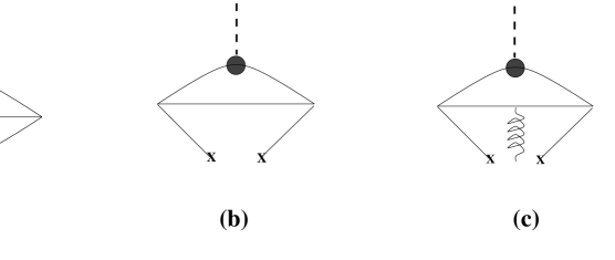
FIG. 1.: The OPE diagrams that we are considering in this work. The solid lines denote quark propagators and the wavy lines denote gluon lines. The blob in each figure denotes the quark-antiquark component interacting with an external meson (either $\pi$ or $\eta$) field specified by the dashed line. In (a),(b),(c),(d), the blob denotes the pseudovector element $A_{\mu}^{q}$ or the pseudotensor element $B_{\mu\nu}^{q}$, and in (e) and (f), it denotes the three-particle wave function Eq. (19).

FIG. 2.: The Borel mass dependence of $a+bM^{2}$ for the $i\gamma_{5}{\hat{p}}$ sum rules in the SU(3) symmetric limit. The continuum threshold $S_{0}=2.07$ GeV², corresponding to the Roper resonance, is used to obtain the solid lines. To see the sensitivity to the continuum threshold, the dashed-lines with $S_{0}=2.57$ GeV² are also plotted.

FIG. 3.: The Borel curves for the $\gamma_{5}\sigma_{\mu\nu}q^{\mu}p^{\nu}$ sum rules in the SU(3) limit. The dashed lines show the sensitivity to the continuum threshold.

FIG. 4.: The Borel curves of the $\gamma_{5}\sigma_{\mu\nu}q^{\mu}p^{\nu}$ sum rules for $\pi\Sigma\Sigma$, $\eta\Sigma\Sigma$, $\pi\Xi\Xi$ and $\eta\Xi\Xi$ when the SU(3) breaking effects are included. The continuum threshold $S_{0}=3$ GeV² has been used for the plots but the sensitivity of the curves to this choice is small.

REFERENCES

- [1] M.A. Shifman, A.I. Vainshtein, and V.I. Zakharov, Nucl. Phys. B 147 (1979) 385, 448.
- [2] L.J. Reinders, H. Rubinstein and S. Yazaki, Phys. Rep. 127 (1985) 1.
- [3] R. Machleidt in Advances in Nuclear Physics, edited by J.W. Negele and E. Vogt (Plenum, New York, 1989), Vol. 19.
- [4] J. J. de Swart, Rev. Mod. Phys. 35 (1963) 916.; 37 (1965) 326 (E).
- [5] V. G. J. Stoks and Th. A. Rijken, Phys. Rev. C 59 (1999) 3009.
- [6] Th. A. Rijken, V. G. J. Stoks and Y. Yamamoto, Phys. Rev. C 59 (1999) 21.
- [7] Hungchong Kim, Su Houng Lee and Makoto Oka, Phys. Lett. B453 (1999) 199.
- [8] Hungchong Kim, Su Houng Lee and Makoto Oka, Phys. Rev. D60 (1999) 034007.
- [9] Hungchong Kim, nucl-th/9904049, Eur. Phys. Jour. A7,(2000), 121.
- [10] Hungchong Kim, Takumi Doi, Makoto Oka and Su Houng Lee, Nucl. Phys. A662 (2000) 371.
- [11] H. Shiomi and T. Hatsuda, Nucl. Phys. A 594 (1995) 294.
- [12] M. C. Birse and B. Krippa, Phys. Lett. B 373 (1996) 9; Phys. Rev. C 54 (1996) 3240.
- [13] L.J. Reinders, H. Rubinstein and S. Yazaki, Nucl. Phys. B 213 (1983) 109.; T. Meissner and E. M. Henley, Phys. Rev. C 55 (1997) 3093.
- [14] K. Maltman, Phys. Rev. C 57 (1998) 69.
- [15] M. E. Bracco, F. S. Navarra and M. Nielsen, Phys. Lett. B454 (1999) 346.
- [16] T. M. Aliev and M. Savci, Phys. Rev. D 61 (1999) 016008.
- [17] B. L. Ioffe, Nucl. Phys. B188 (1981) 317.; B. L. Ioffe and A. V. Smilga, Nucl. Phys. B 232 (1984) 109.
- [18] V. A. Novikov, M. A. Shifman, A. I. Vainshtein and V. I. Zakharov, Fortschr. Phys. 32 (1984) 585.
- [19] J. Pasupathy, J. P. Singh, S. L. Wilson and C. B. Chiu, Phys. Rev. D 36 (1987) 1442.; S. L. Wilson, Ph.D thesis, University of Texas at Austin, 1987.
- [20] V. M. Belyaev, V. M. Braun, A. Khodjamirian and R. Rückl, Phys. Rev. D 51 (1995) 6177.; V. M. Braun and I. B. Filyanov, Z. Phys. C48 (1990) 239.
- [21] V. A. Novikov, M. A. Shifman, A. I. Vainshtein, M. B. Voloshin and V. I. Zakharov, Nucl. Phys. B 237 (1984) 525.
- [22] A. A. Ovchinnikov and A. A. Pivovarov, Sov. J. Nucl. Phys. 48 (1988) 721.
- [23] Hungchong Kim, nucl-th/9906081, To be published in Progress of Theoretical Physics.
- [24] Hungchong Kim, Phys. Rev. C61 (2000) 019801.
- [25] B. Krippa and M. C. Birse, Phys. Rev. C61 (2000) 019802.
- [26] V. L. Chernyak and A. R. Zhitnitsky, Phys. Rep. 112 (1984) 173.
- [27] B. Blok and M. Lublinsky, Phys. Rev. D 57 (1998) 2676.
- [28] P. G. Ratcliffe, Phys. Lett. B365 (1996) 383.; hep-ph/9710458.
- [29] T. Feldmann, P. Kroll and B. Stech, Phys. Rev. D 58 (1998) 114006.
- [30] J. Dey, M. Dey, M. S. Roy, Phys. Lett. B443 (1998) 293.; J. Dey, M. Dey, T. Frederico, L. Tomio, Mod. Phys. Lett. A 12 (1997) 2193.
- [31] A. J. Buchmann and E. M. Henley, nucl-th/9912044.