Interrelation between the isoscalar octupole phonon and the proton-neutron mixed-symmetry quadrupole phonon in near spherical nuclei

Abstract

The interrelation between the octupole phonon and the low-lying proton-neutron mixed-symmetry quadrupole phonon in near-spherical nuclei is investigated. The one-phonon states decay by collective $E3$ and $E2$ transitions to the ground state and by relatively strong $E1$ and $M1$ transitions to the isoscalar $2^{+}_{1}$ state. We apply the proton–neutron version of the Interacting Boson Model including quadrupole and octupole bosons ($sdf$–IBM-2). Two $F$-spin symmetric dynamical symmetry limits of the model, namely the vibrational and the $\gamma$-unstable ones, are considered. We derive analytical formulae for excitation energies as well as $B(E1),B(M1),B(E2)$, and $B(E3)$ values for a number of transitions between low-lying states.

Corresponding author:
Nadya A. Smirnova
Centre de Spectrométrie Nucléaire et de Spectrométrie de Masse,
Bat. 104, Orsay campus, F-91405, France
Tel: (+33) (0)1 69 15 48 57
Fax: (+33) (0)1 69 15 50 08
E-mail: smirnova@csnsm.in2p3.fr

I Introduction

The phonon concept is a useful and simple concept in nuclear structure physics [1]. The low-lying collective $J^{\pi}=2^{+}$ and $3^{-}$ excitations in near-spherical nuclei can be considered as quadrupole and octupole vibrations, which represent the most important vibrational degrees of freedom at low energies. The bosonic phonon concept suggests the occurrence of multiphonon states, which can decay collectively to states with one phonon less by the annihilation of one phonon. In a harmonic picture $n$-phonon states have excitation energies of $n$ times the one-phonon energy. Two of the appealing aspects of the study of multiphonon excitations high above the yrast-line is the investigation of their anharmonicities reflecting the influence of the Pauli principle and higher order residual interactions as well as the interaction of multiphonon modes with single particle degrees of freedom. Certainly these interactions can cause possible fragmentation of the idealized multiphonon modes. This fragmentation or the eventual observation of almost unfragmented multiphonon states can tell how well the considered phonon is an eigenmode of the nuclear dynamical system. To judge the deviation from the idealized multiphonon picture in reality obviously needs the formulation of this idealized situation and the investigation in how far the collective picture can account for the data.

Multiphonon and two-phonon states are at present a very actively investigated topic in nuclear structure physics. A two-quadrupole-phonon ($2^{+}\otimes 2^{+}$) triplet with states having spin and parity quantum numbers $J^{\pi}=0^{+}$, $2^{+}$, $4^{+}$ is usually known in near spherical nuclei. The absence of $J^{\pi}=1^{+},3^{+}$ members of this two-phonon multiplet points at the bosonic character of the identical quadrupole phonons involved. Multi-quadrupole-phonon states (with $n>2$) have also been identified, see e.g. [2, 3, 4]. The investigation and identification of double giant dipole resonances (2GDR), ($3^{-}\otimes 3^{-}$) double-octupole states and ($2^{+}_{\gamma}\otimes 2^{+}_{\gamma}$) double-gamma-vibrations in deformed nuclei are actively debated in the literature, see e.g. Refs. [5, 6, 7, 8, 9, 10, 11].

The mixed-multipolarity ($2^{+}\otimes 3^{-}$) quadrupole-octupole coupled quintuplet [12, 13] with spin and parity quantum numbers $J^{\pi}=1^{-}$ – $5^{-}$ is a very interesting example of the coupling of two different phonons. Members of the ($2^{+}\otimes 3^{-}$) two-phonon quintuplet should decay by definition by collective $E2$ and $E3$ transitions to the $3^{-}_{1}$ octupole phonon state and to the $2^{+}_{1}$ quadrupole phonon state, respectively. The ($2^{+}\otimes 3^{-}$) two-phonon states are expected to occur close to the sum energy $E_{2^{+}\otimes 3^{-}}=E(2^{+}_{1})+E(3^{-}_{1})$. There are only a few examples, e.g. ¹⁴⁴Sm [14], ¹⁴⁴Nd [15, 16], ¹⁴²Ce [17] and ¹¹²Cd [18], where besides the two-phonon $1^{-}$ state other multiplet members have been identified experimentally. The reason might be that all the other states from the $2^{+}\otimes 3^{-}$ quintuplet, except the $1^{-}$, are strongly mixed with non-collective excitations, losing their pure quadrupole–octupole nature. This is supported by shell-model calculations performed recently for $N=82$ nuclei [19]. Thus, the most complete data, which can be used as a testing ground for the concept of quadrupole-octupole coupled two-phonon excitations, are the transition strengths from the mostly unfragmented $1^{-}$ member of the quintuplet.

The $J^{\pi}=1^{-}$ two-phonon state has been very well investigated in magic and near spherical nuclei. In many nuclei, it has been identified close to the sum energy $E_{2^{+}\otimes 3^{-}}$, indicating a quite harmonic phonon coupling [20, 21, 22]. According to its definition, the two-phonon $1^{-}$ state should decay by a collective one-phonon $E2$ transition to the $3^{-}$ octupole phonon state. This has been confirmed experimentally [23, 24]. The collective $1^{-}_{2^{+}\otimes 3^{-}}\to 2^{+}_{1}$ $E3$ transition has not yet been measured due to the possibly dominating $E1$ and $M2$ contaminations in this transition. A particularly interesting feature of the two-phonon $1^{-}$ state is the existence of a relatively strong $E1$ transition to the ground state, which can be sensitively measured in photon scattering experiments [25]. The strength of this two-phonon annihilating $E1$ transition approximately equals the strength of the $3^{-}_{1}\to 2^{+}_{1}$ two-phonon changing $E1$ transition [26] which strongly supports quadrupole-octupole-collective origin of these $E1$ transitions.

All the low-energy one-phonon and two-phonon states mentioned above involve isoscalar phonons. Recently the isovector quadrupole excitation in the valence shell, the $2^{+}_{\rm ms}$ state, has been identified [27] in some nuclei from the measurement of absolute transition strengths, see, e.g., [16, 17, 28, 29, 30, 31, 32, 33]. Isovector excitations in the valence shell form a whole class of low-lying collective states called, more precisely, mixed-symmetry states [34, 35, 36]. The fundamental $2^{+}_{\rm ms}$ state decays by a weakly collective $E2$ transition to the ground state and by a strong $M1$ transition to the isoscalar $2^{+}_{1}$ state, with an $M1$ matrix element of the order of one nuclear magneton [36, 37]. In an harmonic phonon coupling scheme one can expect also the existence of mixed-symmetry two-phonon multiplets, that involve at least one excitation of the mixed-symmetry quadrupole phonon. Two symmetric–mixed-symmetric ($2^{+}_{1}\otimes 2^{+}_{\rm ms}$) two-quadrupole phonon excitations with positive parity, namely a $J^{\pi}=1^{+}$ state (the scissors mode), and a $J^{\pi}=3^{+}$ state have been identified already in the near spherical nucleus ⁹⁴Mo [33, 38]. Similarly one can expect the existence of a ($2^{+}_{\rm ms}\otimes 3^{-}$) mixed-symmetry quadrupole-octupole coupled multiplet with negative parity. In a naive phonon coupling picture members of this quintuplet should show a very complex but, nevertheless, simple to understand decay pattern, which can be predicted from the decay properties of the one-phonon excitations (weakly-collective $E2$ decay and strong $M1$ decay of the $2^{+}_{\rm ms}$ state, and collective $E3$ and relatively strong $E1$ decay of the $3^{-}_{1}$ octupole vibration). For instance, the $J^{\pi}=1^{-}_{2^{+}_{\rm ms}\otimes 3^{-}}$ state should decay by relatively strong $E1$, strong $M1$, weakly-collective $E2$, and collective $E3$ transitions to the ground and to the $1^{+}$ scissors state, to the ordinary, isoscalar ($2^{+}\otimes 3^{-}$) multiplet, and to the one-phonon $3^{-}$ and $2^{+}_{\rm ms}$ states, respectively (see Fig. 1).

Recently, $\gamma$ transitions between the $3^{-}$ octupole phonon state and the $2^{+}_{\rm ms}$ state have been observed experimentally [17, 39] in near spherical nuclei. For an understanding of these new observations it is necessary to investigate the interrelation of the octupole phonon state and the mixed-symmetry $2^{+}_{\rm ms}$ state theoretically. That is one aim of the present article. Another purpose of this article is the proposal of possible two-phonon states generated by the coupling of the octupole degree of freedom with the proton-neutron degree of freedom and the quantitative investigation of the properties of such constructions.

A convenient and sometimes successful approach to new and complicated physical phenomena is the investigation of symmetries and the algebraic solution of symmetric Hamiltonians. In low-energy nuclear structure physics this task can be achieved by application of the algebraic interacting boson model [40, 41]. Since we deal simultaneously with the isoscalar octupole vibration and the isovector quadrupole vibration in the valence shell of near spherical nuclei, we need a model which incorporates them both. We apply for the first time the $sdf$-IBM-2, which considers $l^{\pi}=0^{+}$ monopole ($s$) bosons, $l^{\pi}=2^{+}$ quadrupole ($d$) bosons, $l^{\pi}=3^{-}$ octupole ($f$) bosons, and the proton-neutron ($\pi$ - $\nu$) degree of freedom [34].

In this paper we develop the formalism of the $sdf$-IBM-2 in two particular dynamical symmetry limits relevant for the description of vibrational and $\gamma$-unstable nuclei. In section II we discuss the group reduction chains of the $sdf$-IBM-2 and the quantum numbers, which are necessary to classify the eigenstates of the dynamically symmetric Hamiltonians. We derive analytical formulae for $\gamma$ transition rates. The $E1$ transitions are calculated with a two-body operator. Quadrupole-octupole coupled two-body operators have turned out to be essential for the description of $E1$ transitions generated by quadrupole-octupole collectivity [42, 43, 26].

II $sdf$-IBM-2

The building blocks of the $sdf$-IBM-2 are $2\times 13$ creation and $2\times 13$ annihilation operators

$$b^{+}_{\rho lm},b_{\rho lm}$$ (1)

where $\rho=\pi,\nu$, $l=0,2,3$, $m=0,\pm 1,\ldots,\pm l$, which by definition satisfy standard boson commutation relations:

$$\left[b_{\rho lm},b^{+}_{\rho^{\prime}l^{\prime}m^{\prime}}\right]=\delta_{\rho\rho^{\prime}}\delta_{ll^{\prime}}\delta_{mm^{\prime}}\;.$$ (2)

The total number of bosons is conserved for a given nucleus, i.e.

$$N=N_{\pi}+N_{\nu}=n_{s\pi}+n_{d\pi}+n_{f\pi}+n_{s\nu}+n_{d\nu}+n_{f\nu}\;.$$ (3)

The integers $n_{l\rho}$ in Eq. (3) are the eigenvalues of the boson number operators $\hat{n}_{l\rho}=\left(b^{+}_{\rho l}\cdot\tilde{b}_{\rho l}\right)$, where the dot denotes the scalar product and $\tilde{b}_{\rho lm}=(-1)^{l-m}b_{\rho l,-m}$.

The $2\times 13^{2}=338$ bilinear combinations of proton and neutron boson operators of the type

$$b^{+}_{\rho lm}b_{\rho l^{\prime}m^{\prime}}$$ (4)

generate the Lie algebra U_π(13) $\otimes$ U_ν(13).

A Group reductions, quantum numbers and wave functions

The U_π(13) $\otimes$ U_ν(13) symmetry algebra has a rich substructure. In the present study we are interested in the $F$-spin symmetric dynamical symmetry limits of the model, which can be characterized by the reduction chains

$$\begin{array}[]{ccccccccccccccc}{\mbox{U}_{\pi}(13)}&{\otimes}&{\mbox{U}_{\nu}(13)}&{\supset}&{\mbox{U}_{\pi\nu}(13)}&{\supset}&{\mbox{U}_{\pi\nu}(6)}&{\otimes}&{\mbox{U}_{\pi\nu}(7)}&{\supset\cdots\supset}&{\mbox{SO}^{d}_{\pi\nu}(3)}&{\otimes}&{\mbox{SO}^{f}_{\pi\nu}(3)}&{\supset}&{\mbox{SO}_{\pi\nu}(3)}\\ \downarrow&&\downarrow&&\downarrow&&\downarrow&&\downarrow&&\downarrow&&\downarrow&&\downarrow\\[0.0pt] {[N_{\pi}]}&&{[N_{\nu}]}&&{[N_{1},N_{2}]}&&{[n_{1},n_{2}]}&&{[m_{1},m_{2}]}&{\ldots}&L_{d}&&L_{f}&&L\\ \end{array}$$ (5)

where the dots denote alternative group reductions discussed later. Below each group we indicate the quantum numbers, associated with it. In total, the complete classification of the basis states (5) requires 26 quantum numbers corresponding to the $2\times 13$ occupation numbers $n_{\rho lm}$ in the $m$-scheme. The $F$-spin quantum number [34, 41] relates in terms of Young tableaux to the one- or two-rowed U_πν(13) representation as

$$F=\frac{N_{1}-N_{2}}{2}\;.$$

The maximum value of the $F$-spin quantum number

$$F_{\rm max}=\frac{N}{2}$$

corresponds to the totally symmetric representations of the U_πν(13) group. States with smaller $F$-spin quantum numbers $F<F_{\rm max}$ are called mixed-symmetry states and correspond to non-symmetric representations of the U_πν(13) group. Since the $sdf$-IBM-2 contains an octupole degree of freedom, it enlarges the diversity of mixed-symmetry states compared to the standard $sd$-IBM-2. This fact can be recognized from the branching rules of U_πν(13) $\supset$ U_πν(6) $\otimes$ U_πν(7) (see Appendix A).

The simplest two-rowed representation of U_πν(13) reduces to the U_πν(6) $\supset$ U_πν(7) representations in the following way:

$${\rm U}_{\pi\nu}(13) \supset {\rm U}_{\pi\nu}(6)\otimes{\rm U}_{\pi\nu}(7)$$ (7)

$$[N-1,1] = [n-1,1]\otimes[m]$$ ()

$$[n]\otimes[m-1,1]$$

$$[n]\otimes[m]$$

where, $n=n_{1}+n_{2}$ is the total number of $s$ and $d$ bosons, $m=m_{1}+m_{2}$ is the number of $f$ bosons, giving thus $N=n+m$.

As follows from Eq. (6), three types of the mixed-symmetry states arise.

1. The $[n-1,1]\otimes[m]$ decomposition corresponds to the usual mixed-symmetry states in the $sd$-space, coupled to $m$ octupole-bosons with a wave function, which is symmetric in the $f$-sector. Examples are the fundamental $2^{+}_{\rm ms}$ state and the $1^{+}_{sc}$ “scissors” state with no $f$-boson at all, which belong to the ${\rm U}_{\pi\nu}(6)\otimes{\rm U}_{\pi\nu}(7)$ representation $[n-1,1]\otimes[0]$, or the new negative-parity mixed-symmetry two-phonon states which we denote as $(2^{+}_{\rm ms}\otimes 3^{-}_{1})$ because they are generated by the coupling of the lowest $2^{+}_{\rm ms}$ state in the $sd$-sector and one symmetric $f$-boson, which belong to the ${\rm U}_{\pi\nu}(6)\otimes{\rm U}_{\pi\nu}(7)$ representation $[n-1,1]\otimes[1]$. Note that in the presence of one $f$-boson due to the boson number conservation only $n=N-1$ bosons remain in the $sd$-sector, which can belong to the symmetric ${\rm U}_{\pi\nu}(6)$ representation $[n]=[N-1]$ or to the mixed-symmetry representations, i.e., to the lowest $[n-1,1]=[N-2,1]$. Therefore, the representation $[n-1,1]\otimes[1]$ can be considered as $(2^{+}_{\rm ms}\otimes 3^{-}_{1})$ two-phonon states. It turns out from the application of the branching rules given in Appendix A that this $(2^{+}_{\rm ms}\otimes 3^{-}_{1})$ two-phonon coupling will generate mixed-symmetry states with $F$-spin quantum numbers $F=F_{\rm max}-1$ and $F=F_{\rm max}-2$, because the representation $[N-2,1]\otimes[1]$ is also present in the U_πν(13) representation $[N-2,2]$, which has a total $F$-spin quantum number $F=F_{\rm max}-2$. In this article, we restrict ourselves to mixed-symmetry states with $F=F_{\rm max}-1$.

2. The $[n]\otimes[m-1,1]$ reduction describes the mixed-symmetry states which appear due to mixed-symmetry in the $f$-sector. We will not consider such kind of states in the present paper.

3. Finally, $[n]\otimes[m]$ states are symmetric separately in the $sd$- and in the $f$-sectors, however, they are coupled in a non-symmetric way within the full $sdf$-space. The simplest example for a mixed-symmetry state if this type is the $3^{-}_{\rm ms}$ state, which consists of $m=1$ $f$-boson and $n=N-1$ $s$-bosons. This $3^{-}_{\rm ms}$ state is the mixed-symmetry analogue state of the symmetric octupole phonon, the $3^{-}_{1}$ state. This can be clearly seen from the explicit wave functions given in Table I. Higher excited mixed-symmetry states of this type can be obtained by replacing in a symmetric way $s$-bosons with $d$-bosons in the $3^{-}_{\rm ms}$ wave function along with proper normalization. We denote the lowest energy example of such mixed-symmetry states schematically as $(2^{+}\otimes 3^{-}_{\rm ms})$.

The operator which controls the excitation energy of mixed-symmetry states with $F$-spin quantum numbers $F<F_{\rm max}$ is the Majorana operator. By definition, this is the most general operator which annihilates any totally symmetric state. Within the U_πν(13) $\supset$ U_πν(6) $\otimes$ U_πν(7), there are three important types of Majorana operators.

The well known Majorana operator $\hat{M}_{6}$ [34] is associated with the U(6) group generated by the $s$- and $d$-bosons only. It has the form

$$\hat{M}_{6}=[s^{+}_{\nu}\times d^{+}_{\pi}-s^{+}_{\pi}\times d^{+}_{\nu}]^{(2)}\cdot[s_{\nu}\times\tilde{d}_{\pi}-s_{\pi}\times\tilde{d}_{\nu}]^{(2)}-2\sum_{k=1,3}[d^{+}_{\nu}\times d^{+}_{\pi}]^{(k)}\cdot[\tilde{d}_{\nu}\times\tilde{d}_{\pi}]^{(k)}\;,$$ (8)

which influences the states whose wave functions are non-symmetric in the $sd$-sector of the model space. In Eq. (8) and below, $\times$ denotes the standard tensor product of two irreducible tensorial operators. It relates to the ${\rm U}_{\pi\nu}(6)$ quadratic Casimir operator as

$$C_{2}[\mbox{U}_{\pi\nu}(6)]=n(n+5)-2\hat{M}_{6}\;.$$ (9)

The Majorana operator $\hat{M}_{7}$ is associated with the U(7) group generated by the $f$-bosons only. It has the form

$$\hat{M}_{7}=-2\sum_{k=1,3,5}[f^{+}_{\nu}\times f^{+}_{\pi}]^{(k)}\cdot[\tilde{f}_{\nu}\times\tilde{f}_{\pi}]^{(k)}\$$ (10)

which is responsible for pushing up the mixed-symmetry states of the second type, i.e non-symmetric in the $f$-sector. It relates to the ${\rm U}_{\pi\nu}(7)$ quadratic Casimir invariant as

$$C_{2}[\mbox{U}_{\pi\nu}(7)]=m(m+6)-2\hat{M}_{7}\;.$$ (11)

Finally, the Majorana operator which is associated with the full group U(13), reads

$$\hat{M}_{13} = \hat{M}_{6}+\hat{M}_{7}+[s^{+}_{\nu}\times f^{+}_{\pi}-s^{+}_{\pi}\times f^{+}_{\nu}]^{(3)}\cdot[s_{\nu}\times\tilde{f}_{\pi}-s_{\pi}\times\tilde{f}_{\nu}]^{(3)}$$ (13)

$$+\sum_{k=1,2,3,4,5}(-1)^{k+1}[d^{+}_{\nu}\times f^{+}_{\pi}-d^{+}_{\pi}\times f^{+}_{\nu}]^{(k)}\cdot[\tilde{d}_{\nu}\times\tilde{f}_{\pi}-\tilde{d}_{\pi}\times\tilde{f}_{\nu}]^{(k)}\;,$$

$$= \left[F_{\rm max}\left(F_{\rm max}+1\right)-\hat{F}^{2}\right]\;.$$ (14)

This operator acts on all three types of mixed-symmetry states. $\hat{M}_{13}$ relates to the ${\rm U}_{\pi\nu}(13)$ quadratic Casimir operator as

$$C_{2}[\mbox{U}_{\pi\nu}(13)]=N(N+12)-2\hat{M}_{13}\;.$$ (15)

The most general Hamiltonian constructed from linear and quadratic Casimir operators of the group U_πν(6) $\otimes$ U_πν(7) reads

$$\begin{array}[]{ll}H&=H_{0}+\lambda\hat{M}_{13}+\lambda^{\prime}\hat{M}_{6}+\lambda^{\prime\prime}\hat{M}_{7}+\epsilon_{d}C_{1}[\mbox{U}_{\pi\nu}(5)]+\alpha C_{2}[\mbox{U}_{\pi\nu}(5)]+\kappa^{\prime}C_{2}[\mbox{SU}_{\pi\nu}(3)]\\ &+\eta C_{2}[\mbox{SO}_{\pi\nu}(6)]+\beta C_{2}[\mbox{SO}_{\pi\nu}(5)]+\gamma_{d}C_{2}[\mbox{SO}^{d}_{\pi\nu}(3)]+\epsilon_{f}C_{1}[\mbox{U}_{\pi\nu}(7)]\\ &+\kappa C_{2}[\mbox{SO}_{\pi\nu}(7)]+\xi C_{2}[\mbox{G}_{2\pi\nu}]+\gamma_{f}C_{2}[\mbox{SO}^{f}_{\pi\nu}(3)]+\gamma C_{2}[\mbox{SO}_{\pi\nu}(3)]\;.\end{array}$$ (16)

The definitions of the Casimir invariants of Lie groups used here are given in Appendix B. The structure of the Majorana operators has interesting consequences. The $sdf$-IBM-2 reduces to the simpler version $sdf$-IBM-1, if the strength constant $\lambda$ of the Majorana operator $\hat{M}_{13}$ is set to infinity. Using a finite value of $\lambda$, but $\lambda^{\prime\prime}=\infty$ will remove only those states which have mixed-symmetry in the $f$-sector alone. We will use this choice throughout the paper. For the ordinary mixed-symmetry states in the $sd$-sector, which are known already from the $sd$-IBM-2, the sum $\lambda+\lambda^{\prime}$ plays the role of the ordinary Majorana parameter in the $sd$-IBM-2. The excitation energies of mixed-symmetry states, which contain one $f$-boson are in addition also functions of the quantity $\lambda-\lambda^{\prime}$. This parameter controls the excitation energy of mixed-symmetry states with negative parity.

Since we are going to study vibrational or $\gamma$-unstable nuclei, we are interested in two well-known dynamical symmetry limits of the positive parity $sd$-subchain [41], namely,

$$\mbox{U}_{\pi\nu}(6)\supset\left\{\begin{array}[]{c}\mbox{U}_{\pi\nu}(5)\\ \mbox{SO}_{\pi\nu}(6)\\ \end{array}\right\}\supset\mbox{SO}_{\pi\nu}(5)\supset\mbox{SO}_{\pi\nu}(3)$$ (17)

which we consider in the following subsections.

The negative parity subchain has a unique reduction [44, 45]:

$$\begin{array}[]{ccccccc}\mbox{U}_{\pi\nu}(7)&\supset&\mbox{SO}_{\pi\nu}(7)&\supset&\mbox{G}_{2\pi\nu}&\supset&\mbox{SO}_{\pi\nu}(3)\\ \downarrow&&\downarrow&&\downarrow&&\downarrow\\[0.0pt] [m_{1},m_{2}]&&(\omega_{1},\omega_{2})&&(u_{1},u_{2})&\{\beta_{j}\}&L_{f}\\ \end{array}$$ (18)

where the quantum numbers $\{\beta_{j}\}$ ($j=1,2,3,4$) are the so-called missing labels, which are necessary to classify completely the G${}_{2}\supset$ SO(3) reduction. Unlike the case of $sdf$-IBM-1 where only the totally symmetric representations are important [40, 45], we also deal here with two-rowed representations of the algebras in (5) and (18). This requires some modifications. For example, we have to take into account the exceptional group G₂. For the reduction of not fully symmetric representations of SO(7) the group G₂ helps to resolve the labelling problem. The missing label, which is in general necessary to uniquely define the SO(7) $\supset$ G₂ reduction, is redundant in our case of only two-rowed representations.

1 The U_πν(1)$\otimes$U_πν(5)$\otimes$U_πν(7) dynamical symmetry limit

In this dynamical symmetry limit the reduction chain of the positive parity U_πν(6) subalgebra is [41]

$$\begin{array}[]{ccccccc}\mbox{U}_{\pi\nu}(6)&\supset&\mbox{U}_{\pi\nu}(5)&\supset&\mbox{SO}_{\pi\nu}(5)&\supset&\mbox{SO}^{d}_{\pi\nu}(3)\\ \downarrow&&\downarrow&&\downarrow&&\downarrow\\[0.0pt] [n_{1},n_{2}]&&\{n_{d_{1}},n_{d_{2}}\}&&[\tau_{1},\tau_{2}]&\{\alpha_{i}\}&L_{d}\\ \end{array}$$ (19)

where $\alpha_{i}$ ($i=1,2$) are missing labels, necessary to completely classify the SO(5) $\supset$SO(3) reduction. We denote here $n=n_{1}+n_{2}$ the total number of $s$ and $d$ bosons, while the number of $d$ bosons only is denoted as $n_{d}=n_{d_{1}}+n_{d_{2}}$. Thus, the total wave function can be written as

$${|[N_{\pi}]{\otimes}[N_{\nu}];[N_{1},N_{2}][n_{1},n_{2}]\{n_{d_{1}},n_{d_{2}}\}(\tau_{1},\tau_{2})\{\alpha_{i}\}L_{d};[m_{1},m_{2}](\omega_{1},\omega_{2})(u_{1},u_{2})\{\beta_{j}\}L_{f};LM\rangle}$$ (20)

The quantum numbers of the lowest states are given in Table I.

In the U_πν(5)$\otimes$U_πν(7) dynamical symmetry limit it is rather simple to construct explicitly the wave functions. We shall do this in order to make clear the variety of mixed-symmetry states appearing in the model. In Table I we present the wave functions for some states of interest. We discussed above already the one-$f$-boson octupole states. Of particular interest are here also the lowest $1^{-}$ states. From the coupling of one $d$-boson quadrupole phonon and one $f$-boson octupole phonon four $1^{-}$ states emerge. This is evident in the $m$-scheme in $F$-space because the four basis wave functions $|d_{\pi}f_{\pi}\rangle$, $|d_{\nu}f_{\pi}\rangle$, $|d_{\pi}f_{\nu}\rangle$, and $|d_{\nu}f_{\nu}\rangle$ can be formed. These basis states can be combined to states with U_πν(13) symmetry and good $F$-spin. One obtains one symmetric $1^{-}$ state corresponding to the totally symmetric $[N]$ irrep of U_πν(13) with $F$-spin quantum number $F=F_{\rm max}$, and three mixed-symmetry states: two of them with $F$-spin quantum numbers $F=F_{\rm max}-1$ and one with $F=F_{\rm max}-2$. One $F=F_{\rm max}-1$ state corresponds to the $[N-1,1]\supset[N-2,1]\otimes[1]$ reduction and the other to the $[N-1,1]\supset[N-1]\otimes[1]$ reduction in the U_πν(13)$\supset$ U_πν(6)$\otimes$ U_πν(7), chain. The last one arises from the $[N-2,2]\supset[N-2,1]\otimes[1]$ reduction. According to the discussion above we denote them as $1^{-}=(2^{+}\otimes 3^{-})_{1^{-}}$, $1^{-}_{\rm ms}=(2^{+}_{\rm ms}\otimes 3^{-})_{1^{-}}$, $1^{-\prime}_{\rm ms}=(2^{+}\otimes 3^{-}_{\rm ms})_{1^{-}}$ and $1^{-\prime\prime}_{\rm ms}$, respectively.

The U_πν(5)$\otimes$U_πν(7) dynamical symmetry Hamiltonian expressed in terms of Casimir invariants of first and second order of the relevant groups reads

$$\begin{array}[]{ll}H&=H_{0}+\lambda\hat{M}_{13}+\lambda^{\prime}\hat{M}_{6}+\lambda^{\prime\prime}\hat{M}_{7}+\epsilon_{d}C_{1}[\mbox{U}_{\pi\nu}(5)]\\ &+\alpha C_{2}[\mbox{U}_{\pi\nu}(5)]+\beta C_{2}[\mbox{SO}_{\pi\nu}(5)]+\gamma_{d}C_{2}[\mbox{SO}^{d}_{\pi\nu}(3)]+\epsilon_{f}C_{1}[\mbox{U}_{\pi\nu}(7)]\\ &+\kappa C_{2}[\mbox{SO}_{\pi\nu}(7)]+\xi C_{2}[\mbox{G}_{2\pi\nu}]+\gamma_{f}C_{2}[\mbox{SO}^{f}_{\pi\nu}(3)]+\gamma C_{2}[\mbox{SO}_{\pi\nu}(3)]\;.\end{array}$$ (21)

The eigenvalue problem for the dynamical symmetry Hamiltonian (21) can be solved analytically. The solution of the full U(5) Hamiltonian reads

$$\begin{array}[]{ll}E&=E_{0}+\lambda\left[F_{\rm max}\left(F_{\rm max}+1\right)-F(F+1)\right]+\lambda^{\prime}n_{2}(n_{1}+1)+\lambda^{\prime\prime}m_{2}(m_{1}+1)\\ &+\epsilon_{d}(n_{d_{1}}+n_{d_{2}})+\alpha[n_{d_{1}}(n_{d_{1}}+4)+n_{d_{2}}(n_{d_{2}}+2)]+\beta[\tau_{1}(\tau_{1}+3)+\tau_{2}(\tau_{2}+1)]\\ &+\gamma_{d}L_{d}(L_{d}+1)+\epsilon_{f}(m_{1}+m_{2})+\kappa[\omega_{1}(\omega_{1}+5)+\omega_{2}(\omega_{2}+3)]\\ &+\xi[u_{1}(u_{1}+5)+u_{2}(u_{2}+4)+u_{1}u_{2}]+\gamma_{f}L_{f}(L_{f}+1)+\gamma L(L+1)\;.\end{array}$$ (22)

To construct the spectrum one needs to know the branching rules for the groups involved (see Appendix). An energy spectrum corresponding to (21) is shown in Fig. 2. The parameters of the Hamiltonian are specified in the figure caption.

2 The SO_πν(6)$\otimes$U_πν(7) dynamical symmetry limit

In this dynamical symmetry limit the reduction chain of the positive parity U_πν(6) subalgebra is

$$\begin{array}[]{ccccccc}\mbox{U}_{\pi\nu}(6)&\supset&\mbox{SO}_{\pi\nu}(6)&\supset&\mbox{SO}_{\pi\nu}(5)&\supset&\mbox{SO}^{d}_{\pi\nu}(3)\\ \downarrow&&\downarrow&&\downarrow&&\downarrow\\[0.0pt] [n_{1},n_{2}]&&\langle\sigma_{1},\sigma_{2}\rangle&&[\tau_{1},\tau_{2}]&\{\alpha_{i}\}&L_{d}\\ \end{array}$$ (23)

and the total wave function is as follows:

$${|[N_{\pi}]{\otimes}[N_{\nu}];[N_{1},N_{2}][n_{1},n_{2}]\langle\sigma_{1},\sigma_{2}\rangle(\tau_{1},\tau_{2})\{\alpha_{i}\}L_{d};[m_{1},m_{2}](\omega_{1},\omega_{2})(u_{1},u_{2})\{\beta_{j}\}L_{f};LM\rangle}$$ (24)

The quantum numbers for the lowest states in this dynamical symmetry are presented in Table II.

The SO_πν(6)$\otimes$U_πν(7) dynamical symmetry Hamiltonian reads

$$\begin{array}[]{ll}H&=H_{0}+\lambda\hat{M}_{13}+\lambda^{\prime}\hat{M}_{6}+\lambda^{\prime\prime}\hat{M}_{7}+\zeta C_{2}[\mbox{SO}_{\pi\nu}(6)]\\ &+\beta C_{2}[\mbox{SO}_{\pi\nu}(5)]+\gamma_{d}C_{2}[\mbox{SO}^{d}_{\pi\nu}(3)]+\epsilon_{f}C_{1}[\mbox{U}_{\pi\nu}(7)]\\ &+\kappa C_{2}[\mbox{SO}_{\pi\nu}(7)]+\xi C_{2}[\mbox{G}_{2\pi\nu}]+\gamma_{f}C_{2}[\mbox{SO}^{f}_{\pi\nu}(3)]+\gamma C_{2}[\mbox{SO}_{\pi\nu}(3)]\;.\end{array}$$ (25)

and has the eigenvalues

$$\begin{array}[]{ll}E&=E_{0}+\lambda\left[F_{\rm max}\left(F_{\rm max}+1\right)-F(F+1)\right]+\lambda^{\prime}n_{2}(n_{1}+1)+\lambda^{\prime\prime}m_{2}(m_{1}+1)\\ &+\zeta[\sigma_{1}(\sigma_{1}+4)+\sigma_{2}(\sigma_{2}+2)]+\beta[\tau_{1}(\tau_{1}+3)+\tau_{2}(\tau_{2}+1)]+\gamma_{d}L_{d}(L_{d}+1)\\ &+\epsilon_{f}(m_{1}+m_{2})+\kappa[\omega_{1}(\omega_{1}+5)+\omega_{2}(\omega_{2}+3)]\\ &+\xi[u_{1}(u_{1}+5)+u_{2}(u_{2}+4)+u_{1}u_{2}]+\gamma_{f}L_{f}(L_{f}+1)+\gamma L(L+1)\;.\end{array}$$ (26)

The branching rules for the corresponding groups can be found in Ref. [56] and in the Appendix below. A typical energy spectrum corresponding to Eq. (26) is shown in Fig. 3. The parameters are specified in the caption.

B Electromagnetic transitions

In this subsection we discuss electromagnetic transitions between low-lying states in the $sdf$-IBM-2 with particular emphasis of those transitions which are new in the present model with respect to the standard $sd$-IBM-2 and $sdf$-IBM-1 species. For the study of the interrelation between the $F=F_{\rm max}$ octupole phonon and the $F=F_{\rm max}-1$ mixed-symmetry quadrupole phonon and possible two-phonon states generated by the coupling of them, we are interested in $E1,M1,E2$, and $E3$ transition strengths. The reduced transition probabilities

$$B(\Pi\lambda;J_{i}\to J_{f})=\frac{1}{2J_{i}+1}|\langle J_{f}||T(\Pi\lambda)||J_{i}\rangle|^{2}$$ (27)

are calculated from the matrix elements of the transition operators $T(\Pi\lambda)$, where $\Pi$ stands for the radiation character, either $E$ or $M$, and $\lambda$ denotes the multipolarity.

The electric quadrupole operator reads

$$T(E2)=e_{\pi}Q^{(2)}_{\pi}+e_{\nu}Q^{(2)}_{\nu}\;,$$ (28)

where

$$Q^{(2)}_{\rho}=[d^{+}_{\rho}\times s_{\rho}+s^{+}_{\rho}\times\tilde{d}_{\rho}]^{(2)}+\chi_{\rho}[d^{+}_{\rho}\times\tilde{d}_{\rho}]^{(2)}+\chi^{\prime}_{\rho}[f^{+}_{\rho}\times\tilde{f}_{\rho}]^{(2)}\;.$$ (29)

The magnetic dipole operator has the form

$$T(M1)=\sqrt{\frac{3}{4\pi}}\left(g_{\pi}L^{d}_{\pi}+g_{\nu}L^{d}_{\nu}+g^{\prime}_{\pi}L^{f}_{\pi}+g^{\prime}_{\nu}L^{f}_{\nu}\right)\;,$$ (30)

where

$$L^{d}_{\rho}=\sqrt{10}[d^{+}_{\rho}\times\tilde{d}_{\rho}]^{(1)}\;,\quad L^{f}_{\rho}=2\sqrt{7}[f^{+}_{\rho}\times\tilde{f}_{\rho}]^{(1)}\;.$$ (31)

According to the Eqs. (28–31) the addition of the $f$ boson enlarges the structure of electromagnetic operators of the standard $sd$-IBM-2. The standard $sd$-IBM-2, however, works well for the description of $E2$ and $M1$ transitions. In order to reduce the number of model parameters in the $sdf$-IBM-2 we, therefore, neglect below those parts of the $E2$ and $M1$ transition operators which involve the $f$-boson. Thus, we assume $\chi^{\prime}_{\rho}=0$ and $g^{\prime}_{\rho}=0$. In contrast, the $f$-boson is essential for $E3$ and $E1$ transitions, which are new with respect to the $sd$-IBM-2.

Since there is at present no experimental evidence for the existence of states with mixed-symmetry in the $f$-boson sector, we shall consider here only $F$-scalar octupole transitions, i.e., we use the following symmetric octupole operator:

$$T(E3)=e_{3}\left(O^{(3)}_{\pi}+O^{(3)}_{\nu}\right)\;,$$ (32)

where $O^{(3)}_{\rho}$ stands for

$$O^{(3)}_{\rho}=[s^{+}_{\rho}\times\tilde{f}_{\rho}+f^{+}_{\rho}\times s_{\rho}]^{(3)}+\chi[d^{+}_{\rho}\times\tilde{f}_{\rho}+f^{+}_{\rho}\times\tilde{d}_{\rho}]^{(3)}\;.$$ (33)

The general one-body electric dipole operator has the form

$$T(E1)=\alpha_{\pi}D^{(1)}_{\pi}+\alpha_{\nu}D^{(1)}_{\nu}\;,$$ (34)

where

$$D^{(1)}_{\rho}=\left[d^{+}_{\rho}\times\tilde{f}_{\rho}+f^{+}_{\rho}\times\tilde{d}_{\rho}\right]^{(1)}\;.\\$$ (35)

While the one-body $M1$, $E2$, and $E3$ transition operators work satisfactorily, the one-body $E1$-transition operator fails to provide an adequate description of low-lying dipole transition strengths in vibrational nuclei [42]. This applies for near-spherical nuclei also in the case when a $p$-boson is considered as it will be discussed below. The operator (34) has very strict selection rules, conserving the total number of $d$- and $f$-bosons $\Delta(n_{d}+n_{f})=0$. This contradicts the experimental findings where the quadrupole-octupole collective $E1$ transitions, including the ground state decay of the quadrupole-octupole two-phonon $1^{-}$ state, are even found to be enhanced, see e.g. Refs. [20, 21, 22, 25].

Two approaches exist to avoid this problem. Following the first, the $sdf$-IBM is enlarged with a $p$ boson ($l^{\pi}=1^{-}$), thus leading to the so-called $spdf$-IBM [47, 48, 49, 50]. The inclusion of the $p$ boson in the IBM corresponds to the consideration of a collective dipole vibration. There exists no unambiguous interpretation of the $p$-boson origin. Some authors point out the origin of the $p$-boson from the collective low-lying valence shell excitation after removing the center-of-mass motion [48, 50]. Others have associated the $p$-boson with the GDR [47, 49]. The $p$ boson induced one-body electric dipole operator works succesfully for the description of dipole transition strengths in deformed nuclei [47, 48, 49, 50, 51, 52]. For near-spherical nuclei, where the present article is focussing on, the inclusion of the $p$ boson does not lift all discrepancies [18].

The lowest $1^{-}$ state is the only strong low-lying $E1$ excitation in many near-spherical nuclei [25]. This fact strongly suggests that this state is identified with the collective negative-parity dipole mode in the case of considering a low-energy $p$ boson. This view, however, renders the well-established agreement of the $1^{-}$ excitation energy with the quadrupole-octupole two-phonon sum energy a sheer coincidence. Also the enhanced $E1$ strengths from other members of the quadrupole-octupole coupled quintuplet with spin quantum numbers $J\neq 1$ are not at all simple to understand.

On the other hand some other experimental facts indicate different origin of strong $E1$ transitions in near-spherical nuclei than sheer mixing with the GDR. For example, studies of $E1$-strength distribution in ¹⁴⁰Ce [53] report that the lowest $1^{-}$ state exhibits an enhanced dipole transition to the ground state, while transitions from a number of higher lying $1^{-}$ states are considerably weaker although they lie closer to the GDR and although they are calculated to have predominantly a simple 1p1h-structure, which would even favor a mixing with the GDR. Thus, the observed concentration of $E1$-strength in the lowest $1^{-}$ states should not be simply attributed to admixtures of the GDR into the states wave function if not at the same time the smaller $E1$ strengths of higher lying $1^{-}$ states are explained, too. It is even more striking that a model which can treat all these $E1$ excitations on the same footing, the microscopic Quasiparticle Phonon Model, supports the interpretation of enhanced low-lying $E1$ transitions due to quadrupole-octupole collectivity [54].

Therefore, another approach is preferable. The multiphonon structure of excitations in vibrational nuclei as well as an octupole or quadrupole-octupole coupled origin of negative-parity states, naturally suggests an $E1$-transition operator which contains a quadrupole-octupole coupled two-body part. Such a picture is also supported by the empirical correlation between $E1$-transition strengths of the $1^{-}_{1}\to 0^{+}_{1}$ and $3^{-}_{1}\to 2^{+}_{1}$ transitions found recently for heavy near-spherical nuclei [26] and by the fore-mentioned microscopic calculations [54]. Furthermore, it avoids the problems in connection with the introduction of a $p$ boson discussed above. We choose, therefore, to work with a quadrupole-octupole coupled two-body part in the $E1$ operator.

The two-body dipole operator has already been introduced within the simple quadrupole and octupole phonon model [26] and earlier within the $sdf$-IBM-1 [43, 55]. This ansatz is in good agreement with the available data. The $E1$ transition operator considered here has the form

$$\begin{array}[]{c}\displaystyle T(E1)=\alpha_{\pi}D^{(1)}_{\pi}+\alpha_{\nu}D^{(1)}_{\nu}+\\[3.0pt] \displaystyle\frac{\beta}{2N}\left[\left(Q^{(2)}_{\pi}{+}\eta Q^{(2)}_{\nu}\right){\times}\left(O^{(3)}_{\pi}{+}O^{(3)}_{\nu}\right){+}\left(O^{(3)}_{\pi}{+}O^{(3)}_{\nu}\right){\times}\left(Q^{(2)}_{\pi}{+}\eta Q^{(2)}_{\nu}\right)\right]^{(1)}\;,\end{array}$$ (36)

where $D^{(1)}_{\rho}$, $Q^{(2)}_{\rho}$, and $O^{(3)}_{\rho}$ are given by the Eqs. (35), (29) with $\chi^{\prime}_{\rho}=0$, and (33), respectively, and $\eta=e_{\nu}/e_{\pi}$. We stress that we introduce only one free parameter more ($\beta$) in the $E1$ operator with respect to the one-body operator from Eq. (34). Below we analyze $E1$-transitions within two particular dynamical symmetry limits.

1 The U_πν(1)$\otimes$U_πν(5)$\otimes$U_πν(7) dynamical symmetry limit

Using the wave functions (20) we can obtain the matrix elements of the transition operators (28), (30), (32) and (36). The technique for the calculation of such matrix elements is described in detail in Ref. [56]. In this particular dynamical symmetry limit, it is more convenient to use the explicit expressions of the wave functions constructed from boson operators following the method described in [57] (see, e.g., Ref. [56]). The $E2$ and $M1$ transition strengths between those states, whose wave functions do not involve any $f$ bosons, are exactly the same as in the case of the $sd$-IBM-2 and can be found in [56]. The advantage of the $sdf$-IBM-2 is that it provides the description of $E2$ and $M1$ transitions between negative parity states and of $E1$ and $E3$ transitions between the states of different parity and different $F$-spin. Here we are particularly interested in the electric dipole transitions which connect the octupole $3_{1}^{-}$ state with the symmetric $2^{+}_{1}$ state and with the mixed-symmetry $2_{\rm ms}^{+}$ state, as well as in those which connect the $(2^{+}\otimes 3^{-})$ two-phonon negative parity multiplet with the ground state band. We also consider here the new mixed-symmetry quadrupole-octupole coupled dipole states $1^{-}_{\rm ms}=(2^{+}_{\rm ms}\otimes 3^{-})_{1^{-}}$ and $1^{-\prime}_{\rm ms}=(2^{+}\otimes 3^{-}_{\rm ms})_{1^{-}}$ and their electromagnetic properties (including $M1$ strengths) as examples for mixed-symmetry states with negative parity. Analytical expressions of reduced transition probabilities are summarized in Table III.

It is worthwhile to look closely to the analytical expressions in Table III in order recognize the fingerprints of the simple phonon picture the consideration of which has guided us to the present model. The $E1$ transition strengths from the $3^{-}_{1}$ state to the symmetric and mixed-symmetry one-phonon quadrupole excitations, the $2^{+}_{1}$ state and the $2^{+}_{\rm ms}$ state, are both of the order of $(1/N)^{0}$, i.e., they can be strong on an absolute scale and comparable. The $3^{-}_{1}\to 2^{+}_{\rm ms}$ $F$-vector $E1$ strength can be even larger than that of the strong $F$-scalar $3^{-}_{1}\to 2^{+}_{1}$ $E1$ transition if the effective electric dipole charges $\alpha_{\pi}$ and $\alpha_{\nu}$ have opposite signs. Similarly, the $E1$ ground state excitation strengths to the $1^{-}_{1}$ state and the $1^{-}_{\rm ms}$ state are both of the order of $(1/N)^{0}$ due to the two-body part of the $E1$ operator. However, here the $F$-scalar $0^{+}_{1}\to 1^{-}_{1}$ $E1$ strength must be expected to be larger than the $F$-vector $E1$ strength of the $0^{+}_{1}\to 1^{-}_{\rm ms}$ transition because the parameter $\eta$ usually takes values between 0 and 1 leading to a reduction of the $F$-vector $E1$ strength which is proportional to the factor $(1-\eta)^{2}$. It is also interesting to compare the properties of the new mixed-symmetry $1^{-}$ states, $1^{-}_{\rm ms}$ and $1^{-\prime}_{\rm ms}$. The direct $E1$ ground state excitation strengths to the $1^{-\prime}_{\rm ms}$ state is only of the order of $(1/N)^{2}$ and therefore much smaller than the $E1$ strength to the $1^{-}_{\rm ms}$ state, which is of the order of $(1/N)^{0}$. The $1^{-}_{\rm ms}\to 3^{-}_{1}$ $E2$ strength is of the order of N, which indicates quadrupole collectivity. Since it is proportional to the square of the difference of the effective quadrupole boson charges $(e_{\pi}-e_{\nu})^{2}$ this transition should be weakly collective like the known $2^{+}_{\rm ms}\to 0^{+}_{1}$ one-quadrupole phonon decay. In contrast, the $1^{-\prime}_{\rm ms}\to 3^{-}_{1}$ $E2$ strength is of the order of $1/N$ and cannot be large. Very interesting are also the $M1$ transitions between symmetric and mixed-symmetry negative parity states. The $M1$ strengths from the $1^{-}_{\rm ms}$ state to the quadrupole-octupole coupled $1^{-}$ and $2^{-}$ two-phonon states are of the order of $(1/N)^{0}$ and should be comparable to the $2^{+}_{\rm ms}\to 2^{+}_{1}$ strong $M1$ transition. The $1^{-\prime}_{\rm ms}\to 1^{-},2^{-}$ $M1$ transitions are of the order of $(1/N)^{2}$ if the $d$-boson part alone is used in the $M1$ transition operator (30). If one allows for finite $g$-factors $g^{\prime}_{\rho}$ for the $f$-boson parts in the $M1$ operator (30), they will be responsible for the leading term of the order of $(1/N)^{0}$ which was therefore included in Table III. This resembles the fact that the $1^{-\prime}_{\rm ms}$ state originates from the non symmetric coupling of an $f$-boson to the $sd$-sector. In summary the $1^{-}_{\rm ms}$ state shows the behavior, which is mentioned in the introduction to be expected for a two-phonon state formed by the coupling of the fundamental phonons which generate the $3^{-}_{1}$ state and the $2^{+}_{\rm ms}$ state.

2 The SO_πν(6)$\otimes$U_πν(7) dynamical symmetry limit

Using the wave functions (24) we have calculated the matrix elements of the transition operators (28), (30), (32) and (36). We use here the quadrupole operator (29) with $\chi_{\rho}=0$ as is conventional for the SO(6) limit. The analytical expressions for the $E2$ and $M1$ transitions between the states which are formed only from $s$ and $d$ bosons are identical to those of the $sd$-IBM-2 and can be found in Ref. [56]. Analytical expressions for $E2$ and $M1$ transition strengths between negative parity states and for $E1$ and $E3$ transition strengths are summarized in Table IV.

III Summary

The relation and coupling of the collective octupole degree of freedom to proton-neutron mixed-symmetry states is discussed in the framework of the interacting boson model. For this purpose $s$-bosons, $d$-bosons, and $f$-bosons as well as the proton-neutron degree of freedom had to be taken into account leading to the hitherto not considered $sdf$-IBM-2 version of the model. We developed the formalism of the $sdf$-IBM-2 considering two $F$-spin symmetric dynamical symmetry limits which are denoted by U_πν(5)$\otimes$U_πν(7) and SO_πν(6)$\otimes$U_πν(7). These analytically solvable limits of the model can be relevant for the description of near spherical, vibrational and $\gamma$-unstable nuclei, respectively. The full dynamically symmetric Hamiltonians are formulated, their eigenstates are specified and the analytical expressions for their excitation energies are given. Low-lying, collective, negative parity states are discussed including for the first time negative parity mixed-symmetry states. Analytical expressions for $E1$, $M1$, $E2$, and $E3$ transition strengths were evaluated. The $E1$ operator considered here contains a quadrupole-octupole coupled two-body part besides the one-body term. Evidence for the possible dominance of $F$-vector $E1$ transitions over $F$-scalar $E1$ transitions is found. The decay properties of $1^{-}_{\rm ms}$ states in vibrational nuclei are predicted.

A U(13)$\supset$ U(6)$\otimes$U(7) branching rules

In order to provide a complete classification scheme we need to reduce the representations of U(13) group to the Kronecker product U(6)$\otimes$U(7). Here we present the branching rules only for the totally symmetric $[N]$ and the lowest mixed-symmetry $[N-1,1]$ and $[N-2,2]$ irreducible representations of U(13). The U(6)$\otimes$U(7) representations are denoted as $[\alpha]\otimes[\beta]$. Those U(6)$\otimes$U(7) decompositions, which contain $1^{-}$ states discussed in the text, are underlined.

$$\begin{array}[]{ll}[N]=&[N]\otimes[0],\;\underline{[N-1]\otimes[1]},\ldots,[1]\otimes[N-1],\;[0]\otimes[N]\\[2.0pt] [N-1,1]=&[N-1,1]\otimes[0],\;\underline{[N-2,1]\otimes[1]},\ldots,[2,1]\otimes[N-3],\;[1,1]\otimes[N-2]\\ &\underline{[N-1]\otimes[1]},\;[N-2]\otimes[2],\ldots,[2]\otimes[N-2],\;[1]\otimes[N-1]\\ &[N-2]\otimes[1,1],\;[N-3]\otimes[2,1],\ldots,[1]\otimes[N-2,1],\;[0]\otimes[N-1,1]\\[2.0pt] [N-2,2]=&[N-2,2]\otimes[0],\;[N-3,2]\otimes[1],\ldots,[3,2]\otimes[N-5],\;[2,2]\otimes[N-4]\\ &\underline{[N-2,1]\otimes[1]},\;[N-3,1]\otimes[2],\ldots,[3,1]\otimes[N-4],\;[2,1]\otimes[N-3]\\ &[N-2]\otimes[2],\;[N-3]\otimes[3],\ldots,[3]\otimes[N-3],\;[2]\otimes[N-2]\\ &[N-3,1]\otimes[1,1],\;[N-4,1]\otimes[2,1],\ldots,\;[2,1]\otimes[N-4,1],\;[1,1]\otimes[N-3,1]\\ &[N-3]\otimes[2,1],\;[N-4]\otimes[3,1],\ldots,[2]\otimes[N-3,1],\;[1]\otimes[N-2,1]\\ &[N-4]\otimes[2,2],\;[N-5]\otimes[3,2],\ldots,[1]\otimes[N-3,2],\;[0]\otimes[N-2,2]\\[2.0pt] \end{array}$$ (A1)

The branching rules for the chains U(6)$\supset$ U(5)$\supset$ SO(5) $\supset$SO(3) and U(6)$\supset$ SO(6)$\supset$ SO(5) $\supset$SO(3) reduction chains can be found elsewhere [41]. The partial classification scheme for the chain U(7)$\supset$ SO(7)$\supset$G₂ $\supset$SO(3) is given in Table VII.

B Casimir invariants

The Casimir invariants of Lie algebras exploited here can be expressed in terms of boson creation and annihilation operators as follows [41]:

$$\begin{array}[]{ll}C_{1}\left[\mbox{U(7)}\right]=&\left(f^{+}\cdot\tilde{f}\right)\;,\\ C_{2}\left[\mbox{U(7)}\right]=&\sum\limits_{K=0}^{6}\left[f^{+}\times\tilde{f}\right]^{(K)}\cdot\left[f^{+}\times\tilde{f}\right]^{(K)}\;,\\ C_{1}\left[\mbox{U(6)}\right]=&\left(s^{+}\cdot s\right)+\left(d^{+}\cdot\tilde{d}\right)\;,\\ C_{2}\left[\mbox{U(6)}\right]=&(s^{+}\cdot s)\cdot(s^{+}\cdot s)+\sum\limits_{K=0}^{4}\left[d^{+}\times\tilde{d}\right]^{(K)}\cdot\left[d^{+}\times\tilde{d}\right]^{(K)}\;,\\ C_{2}\left[\mbox{SU(3)}\right]=&2\left(\left[d^{+}{\times}s+s^{+}{\times}\tilde{d}\right]^{(2)}-\frac{\sqrt{7}}{2}\left[d^{+}{\times}\tilde{d}\right]^{(2)}\right)\left(\left[d^{+}{\times}s+s^{+}{\times}\tilde{d}\right]^{(2)}-\frac{\sqrt{7}}{2}\left[d^{+}{\times}\tilde{d}\right]^{(2)}\right)\\ &+\frac{15}{2}\left[d^{+}{\times}\tilde{d}\right]^{(1)}\cdot\left[d^{+}{\times}\tilde{d}\right]^{(1)}\;,\\ C_{2}\left[\mbox{SO(7)}\right]=&\sum\limits_{K=1,3,5,7}\left[f^{+}\times\tilde{f}\right]^{(K)}\cdot\left[f^{+}\times\tilde{f}\right]^{(K)}\;,\\ C_{2}\left[\mbox{SO(6)}\right]=&\left[d^{+}{\times}s+s^{+}{\times}\tilde{d}\right]^{(2)}\cdot\left[d^{+}{\times}s+s^{+}{\times}\tilde{d}\right]^{(2)}+2\sum\limits_{K=1,3}\left[d^{+}{\times}\tilde{d}\right]^{(K)}\cdot\left[d^{+}{\times}\tilde{d}\right]^{(K)}\;,\\ C_{2}\left[\mbox{SO(5)}\right]=&\sum\limits_{K=1,3}\left[d^{+}\times\tilde{d}\right]^{(K)}\cdot\left[d^{+}\times\tilde{d}\right]^{(K)}\;,\\ C_{2}\left[\mbox{SO${}^{d}$(3)}\right]=&10\left[d^{+}\times\tilde{d}\right]^{(1)}\cdot\left[d^{+}\times\tilde{d}\right]^{(1)}\;,\\ C_{2}\left[\mbox{SO${}^{f}$(3)}\right]=&28\left[f^{+}\times\tilde{f}\right]^{(1)}\cdot\left[f^{+}\times\tilde{f}\right]^{(1)}\;,\\ C_{2}\left[\mbox{G}_{2}\right]=&\sum\limits_{K=1,5}\left[f^{+}{\times}\tilde{f}\right]^{(K)}\cdot\left[f^{+}{\times}\tilde{f}\right]^{(K)}\;.\\ \end{array}$$ (B1)

The exceptional algebra G₂ has been introduced in physics by Racah [44]. The eigenvalues of the Casimir invariants from (B1) in an irreducible representation given by a $[f_{1}f_{2}\ldots f_{n}]$ Young tableau are

$$\begin{array}[]{l}\langle C_{1}\left[\mbox{U}(n)\right]\rangle=\sum\limits_{i=1}^{n}f_{i}\;,\\ \langle C_{2}\left[\mbox{U}(n)\right]\rangle=\sum\limits_{i=1}^{n}f_{i}(f_{i}+n+1-2i)\;,\\ \langle C_{2}\left[\mbox{SU(3)}\right]\rangle=\lambda^{2}+\mu^{2}+\lambda\mu+3\lambda+3\mu\;,\qquad(\lambda=f_{1}-f_{2},\mu=f_{2})\\ \langle C_{2}\left[\mbox{SO}(2n+1)\right]\rangle=\sum\limits_{i=1}^{n}2f_{i}(f_{i}+2n+1-2i)\;,\\ \langle C_{2}\left[\mbox{SO}(2n)\right]\rangle=\sum\limits_{i=1}^{n}2f_{i}(f_{i}+2n-2i)\;,\\ \langle C_{2}\left[\mbox{G}_{2}\right]\rangle=f_{1}(f_{1}+5)+f_{2}(f_{2}+4)+f_{1}f_{2}\;.\end{array}$$ (B2)

TABLE I.: Notation for some low-lying states in the U_πν(1)$\otimes$U_πν(5)$\otimes$U_πν(7) dynamical symmetry limit.

	${{|[N_{\pi}]{\otimes}[N_{\nu}];[N_{1},N_{2}],[n_{1},n_{2}]\{n_{d_{1}},n_{d_{2}}\}(\tau_{1},\tau_{2})\{\alpha_{i}\}L_{d};[m_{1},m_{2}](\omega_{1},\omega_{2})(u_{1},u_{2})\{\beta_{j}\}L_{f};L\rangle}}$
$|0^{+}_{1}\rangle$	= $|[N_{\pi}]\otimes[N_{\nu}];[N],[N]\{0\}(0)0;[0](0)(0)0;0\rangle=|s_{\pi}^{N_{\pi}}s_{\nu}^{N_{\nu}};0\rangle$
$|0^{+}_{2}\rangle$	$=|[N_{\pi}]\otimes[N_{\nu}];[N],[N]\{2\}(0)0;[0](0)(0)0;0\rangle$
	$=(N(N-1))^{-1/2}\left(\sqrt{N_{\pi}(N_{\pi}-1)}|d_{\pi}^{2};0\rangle+\sqrt{2N_{\nu}N_{\pi}}|d_{\pi}d_{\nu};0\rangle+\sqrt{N_{\nu}(N_{\nu}-1)}|d_{\nu}^{2};0\rangle\right)$
$|1^{+}_{\rm ms}\rangle$	$=|[N_{\pi}]\otimes[N_{\nu}];[N-1,1],[N-1,1]\{1,1\}(1,1)1;[0](0)(0)0;1\rangle$
	$=|d_{\pi}d_{\nu};1\rangle$
$|2^{+}_{1}\rangle$	$=|[N_{\pi}]\otimes[N_{\nu}];[N],[N]\{1\}(1)2;[0](0)(0)0;2\rangle$
	$=N^{-1/2}\left(\sqrt{N_{\pi}}|d_{\pi};2\rangle+\sqrt{N_{\nu}}|d_{\nu};2\rangle\right)$
$|2^{+}_{2}\rangle$	$=|[N_{\pi}]\otimes[N_{\nu}];[N],[N]\{2\}(2)2;[0](0)(0)0;2\rangle$
	$=(N(N-1))^{-1/2}\left(\sqrt{N_{\pi}(N_{\pi}-1)}|d_{\pi}^{2};2\rangle+\sqrt{2N_{\nu}N_{\pi}}|d_{\pi}d_{\nu};2\rangle+\sqrt{N_{\nu}(N_{\nu}-1)}|d_{\nu}^{2};2\rangle\right)$
$|2^{+}_{\rm ms}\rangle$	$=|[N_{\pi}]\otimes[N_{\nu}];[N-1,1],[N-1,1]\{1\}(1)2;[0](0)(0)0;2\rangle$
	$=N^{-1/2}\left(\sqrt{N_{\nu}}|d_{\pi};2\rangle-\sqrt{N_{\pi}}|d_{\nu};2\rangle\right)$
$|3^{+}_{1}\rangle$	$=|[N_{\pi}]\otimes[N_{\nu}];[N],[N]\{3\}(3)3;[0](0)(0)0;3\rangle$
	$=(N(N-1)(N-2))^{-1/2}\left(\sqrt{N_{\pi}(N_{\pi}-1)(N_{\pi}-2)}|d_{\pi}^{3};3\rangle+\sqrt{N_{\nu}(N_{\nu}-1)(N_{\nu}-2)}|d_{\nu}^{3};3\rangle\right.$
	$+\sqrt{3N_{\pi}(N_{\pi}-1)N_{\nu}}\left(\sqrt{\frac{5}{7}}|d_{\pi}(2)d_{\nu};3\rangle-\sqrt{\frac{2}{7}}|d_{\pi}(4)d_{\nu};3\rangle\right)$
	$\left.+\sqrt{3N_{\pi}N_{\nu}(N_{\nu}-1)}\left(\sqrt{\frac{5}{7}}|d_{\nu}(2)d_{\pi};3\rangle-\sqrt{\frac{2}{7}}|d_{\nu}(4)d_{\pi};3\rangle\right)\right)$
$|3^{+}_{\rm ms}\rangle$	$=|[N_{\pi}]\otimes[N_{\nu}];[N-1,1],[N-1,1]\{1,1\}(1,1)3;[0](0)(0)0;3\rangle$
	$=|d_{\pi}d_{\nu};3\rangle$
$|4^{+}_{1}\rangle$	$=|[N_{\pi}]\otimes[N_{\nu}];[N],[N]\{2\}(2)4;[0](0)(0)0;4\rangle$
	$=(N(N-1))^{-1/2}\left(\sqrt{N_{\pi}(N_{\pi}-1)}|d_{\pi}^{2};4\rangle+\sqrt{2N_{\nu}N_{\pi}}|d_{\pi}d_{\nu};4\rangle+\sqrt{N_{\nu}(N_{\nu}-1)}|d_{\nu}^{2};4\rangle\right)$
$|6^{+}_{1}\rangle$	$=|[N_{\pi}]\otimes[N_{\nu}];[N],[N]\{3\}(3)6;[0](0)(0)0;6\rangle$
	$=(N(N-1)(N-2))^{-1/2}\left(\sqrt{N_{\pi}(N_{\pi}-1)(N_{\pi}-2)}|d_{\pi}^{3};6\rangle+\sqrt{N_{\nu}(N_{\nu}-1)(N_{\nu}-2)}|d_{\nu}^{3};6\rangle\right.$
	$+\sqrt{3N_{\pi}(N_{\pi}-1)N_{\nu}}\left(\sqrt{\frac{5}{7}}|d_{\pi}(2)d_{\nu};6\rangle-\sqrt{\frac{2}{7}}|d_{\pi}(4)d_{\nu};6\rangle\right)$
	$\left.+\sqrt{3N_{\pi}N_{\nu}(N_{\nu}-1)}\left(\sqrt{\frac{5}{7}}|d_{\nu}(2)d_{\pi};6\rangle-\sqrt{\frac{2}{7}}|d_{\nu}(4)d_{\pi};6\rangle\right)\right)$
$|3^{-}_{1}\rangle$	$=|[N_{\pi}]\otimes[N_{\nu}];[N],[N-1]\{0\}(0)0;[1](1)(1)3;3\rangle$
	$=N^{-1/2}\left(\sqrt{N_{\pi}}|f_{\pi};3\rangle+\sqrt{N_{\nu}}|f_{\nu};3\rangle\right)$
$|3^{-}_{\rm ms}\rangle$	$=|[N_{\pi}]\otimes[N_{\nu}];[N-1,1],[N-1]\{0\}(0)0;[1](1)(1)3;3\rangle$
	$=N^{-1/2}\left(\sqrt{N_{\nu}}|f_{\pi};3\rangle-\sqrt{N_{\pi}}|f_{\nu};3\rangle\right)$
$|1^{-}_{1}\rangle$	$=|[N_{\pi}]\otimes[N_{\nu}];[N],[N-1]\{1\}(1)2;[1](1)(1)3;1\rangle$
	$=(N(N-1))^{-1/2}\left(\sqrt{N_{\pi}(N_{\pi}-1)}|d_{\pi}f_{\pi};1\rangle+\sqrt{N_{\nu}(N_{\nu}-1)}|d_{\nu}f_{\nu};1\rangle\right.$
	$\left.+\sqrt{N_{\nu}N_{\pi}}|d_{\pi}f_{\nu};1\rangle+\sqrt{N_{\nu}N_{\pi}}|d_{\nu}f_{\pi};1\rangle\right)$
$|1^{-}_{\rm ms}\rangle$	$=|[N_{\pi}]\otimes[N_{\nu}];[N-1,1],[N-2,1]\{1\}(1)2;[1](1)(1)3;1\rangle$
	$=((N-1)(N-2))^{-1/2}\left(\sqrt{N_{\nu}(N_{\pi}-1)}|d_{\pi}f_{\pi};1\rangle-\sqrt{N_{\pi}(N_{\nu}-1)}|d_{\nu}f_{\nu};1\rangle\right.$
	$\left.+(N_{\nu}-1)|d_{\pi}f_{\nu};1\rangle-(N_{\pi}-1)|d_{\nu}f_{\pi};1\rangle\right)$
$|1^{-\prime}_{\rm ms}\rangle$	$=|[N_{\pi}]\otimes[N_{\nu}];[N-1,1],[N-1]\{1\}(1)2;[1](1)(1)3;1\rangle$
	$=(N(N-1))^{-1/2}\left(\sqrt{N_{\nu}(N_{\pi}-1)}|d_{\pi}f_{\pi};1\rangle-\sqrt{N_{\pi}(N_{\nu}-1)}|d_{\nu}f_{\nu};1\rangle\right.$
	$\left.-N_{\pi}|d_{\pi}f_{\nu};1\rangle+N_{\nu}|d_{\nu}f_{\pi};1\rangle\right)$
$|1^{-\prime\prime}_{\rm ms}\rangle$	$=|[N_{\pi}]\otimes[N_{\nu}];[N-2,2],[N-2,1]\{1\}(1)2;[1](1)(1)3;1\rangle$
	$=((N-1)(N-2))^{-1/2}\left(-\sqrt{N_{\nu}(N_{\nu}-1)}|d_{\pi}f_{\pi};1\rangle-\sqrt{N_{\pi}(N_{\pi}-1)}|d_{\nu}f_{\nu};1\rangle\right.$
	$\left.+\sqrt{(N_{\pi}-1)(N_{\nu}-1)}|d_{\pi}f_{\nu};1\rangle+\sqrt{(N_{\pi}-1)(N_{\nu}-1)}|d_{\nu}f_{\pi};1\rangle\right)$
$|2^{-}_{1}\rangle$	$=|[N_{\pi}]\otimes[N_{\nu}];[N],[N-1]\{1\}(1)2;[1](1)(1)3;2\rangle$
	$=(N(N-1))^{-1/2}\left(\sqrt{N_{\pi}(N_{\pi}-1)}|d_{\pi}f_{\pi};2\rangle+\sqrt{N_{\nu}(N_{\nu}-1)}|d_{\nu}f_{\nu};2\rangle\right.$
	$\left.+\sqrt{N_{\nu}N_{\pi}}|d_{\pi}f_{\nu};2\rangle+\sqrt{N_{\nu}N_{\pi}}|d_{\nu}f_{\pi};2\rangle\right)$
$|3^{-}_{2}\rangle$	= $|[N_{\pi}]\otimes[N_{\nu}];[N],[N-1]\{1\}(1)2;[1](1)(1)3;3\rangle$
	$=(N(N-1))^{-1/2}\left(\sqrt{N_{\pi}(N_{\pi}-1)}|d_{\pi}f_{\pi};3\rangle+\sqrt{N_{\nu}(N_{\nu}-1)}|d_{\nu}f_{\nu};3\rangle\right.$
	$\left.+\sqrt{N_{\nu}N_{\pi}}|d_{\pi}f_{\nu};3\rangle+\sqrt{N_{\nu}N_{\pi}}|d_{\nu}f_{\pi};3\rangle\right)$
$|4^{-}_{1}\rangle$	$=|[N_{\pi}]\otimes[N_{\nu}];[N],[N-1]\{1\}(1)2;[1](1)(1)3;4\rangle$
	$=(N(N-1))^{-1/2}\left(\sqrt{N_{\pi}(N_{\pi}-1)}|d_{\pi}f_{\pi};4\rangle+\sqrt{N_{\nu}(N_{\nu}-1)}|d_{\nu}f_{\nu};4\rangle\right.$
	$\left.+\sqrt{N_{\nu}N_{\pi}}|d_{\pi}f_{\nu};4\rangle+\sqrt{N_{\nu}N_{\pi}}|d_{\nu}f_{\pi};4\rangle\right)$
$|5^{-}_{1}\rangle$	$=|[N_{\pi}]\otimes[N_{\nu}];[N],[N-1]\{1\}(1)2;[1](1)(1)3;5\rangle$
	$=(N(N-1))^{-1/2}\left(\sqrt{N_{\pi}(N_{\pi}-1)}|d_{\pi}f_{\pi};5\rangle+\sqrt{N_{\nu}(N_{\nu}-1)}|d_{\nu}f_{\nu};5\rangle\right.$
	$\left.+\sqrt{N_{\nu}N_{\pi}}|d_{\pi}f_{\nu};5\rangle+\sqrt{N_{\nu}N_{\pi}}|d_{\nu}f_{\pi};5\rangle\right)$

TABLE II.: Notation for some low-lying states in the SO_πν(6)$\otimes$U_πν(7) dynamical symmetry limit.

${{|[N_{\pi}]{\otimes}[N_{\nu}];[N_{1},N_{2}],[n_{1},n_{2}]\langle\sigma_{1},\sigma_{2}\rangle(\tau_{1},\tau_{2})\{\alpha_{i}\}L_{d};[m_{1},m_{2}](\omega_{1},\omega_{2})(u_{1},u_{2})\{\beta_{j}\}L_{f};LM\rangle}}$
$|0^{+}_{1}\rangle=|[N_{\pi}]\otimes[N_{\nu}];[N],[N]\langle N\rangle(0)0;[0](0)(0)0;0\rangle$
$|0^{+}_{2}\rangle=|[N_{\pi}]\otimes[N_{\nu}];[N],[N]\langle N\rangle(2)0;[0](0)(0)0;0\rangle$
$|1^{+}_{\rm ms}\rangle=|[N_{\pi}]\otimes[N_{\nu}];[N-1,1],[N-1,1]\langle N-1,1\rangle(1,1)1;[0](0)(0)0;1\rangle$
$|2^{+}_{1}\rangle=|[N_{\pi}]\otimes[N_{\nu}];[N],[N]\langle N\rangle(1)2;[0](0)(0)0;2\rangle$
$|2^{+}_{2}\rangle=|[N_{\pi}]\otimes[N_{\nu}];[N],[N]\langle N\rangle(2)2;[0](0)(0)0;2\rangle$
$|2^{+}_{\rm ms}\rangle=|[N_{\pi}]\otimes[N_{\nu}];[N-1,1],[N-1,1]\langle N-1,1\rangle(1)2;[0](0)(0)0;2\rangle$
$|3^{+}_{\rm ms}\rangle=|[N_{\pi}]\otimes[N_{\nu}];[N-1,1],[N-1,1]\langle N-1,1\rangle(1,1)3;[0](0)(0)0;3\rangle$
$|4^{+}_{1}\rangle=|[N_{\pi}]\otimes[N_{\nu}];[N],[N]\langle 2\rangle(2)4;[0](0)(0)0;4\rangle$
$|3^{-}_{1}\rangle=|[N_{\pi}]\otimes[N_{\nu}];[N],[N-1]\langle N-1\rangle(0)0;[1](1)(1)3;3\rangle$
$|3^{-\prime}_{\rm ms}\rangle=|[N_{\pi}]\otimes[N_{\nu}];[N-1,1],[N-1]\langle N-1\rangle(0)0;[1](1)(1)3;3\rangle$
$|1^{-}_{1}\rangle=|[N_{\pi}]\otimes[N_{\nu}];[N],[N-1]\langle N-1\rangle(1)2;[1](1)(1)3;1\rangle$
$|1^{-}_{\rm ms}\rangle=|[N_{\pi}]\otimes[N_{\nu}];[N-1,1],[N-2,1]\langle N-2,1\rangle(1)2;[1](1)(1)3;1\rangle$
$|1^{-\prime}_{\rm ms}\rangle=|[N_{\pi}]\otimes[N_{\nu}];[N-1,1],[N-1]\langle N-1\rangle(1)2;[1](1)(1)3;1\rangle$
$|1^{-\prime\prime}_{\rm ms}\rangle=|[N_{\pi}]\otimes[N_{\nu}];[N-2,2],[N-2,1]\langle N-2,1\rangle(1)2;[1](1)(1)3;1\rangle$

TABLE III.: Some analytical expressions for reduced electromagnetic transition strengths in the U_πν(1)$\otimes$U_πν(5)$\otimes$U_πν(7) dynamical symmetry limit.

$B(E3;0^{+}_{1}\to 3^{-}_{1})$	=	$7e_{3}^{2}N$
$B(E1;3^{-}_{1}\to 2^{+}_{1})$	=	$\frac{3}{7}\left[(\alpha_{\nu}N_{\nu}+\alpha_{\pi}N_{\pi})\frac{1}{N}+\beta\left(N_{\pi}+\eta N_{\nu}\right)\frac{2\,N-1}{2N^{2}}+\sqrt{{6\over{35}}}\beta\chi\left(\chi_{\pi}N_{\pi}+\chi_{\nu}\eta N_{\nu}\right)\frac{1}{N^{2}}\right]^{2}$
$B(E1;3^{-}_{1}\to 2^{+}_{\rm ms})$	=	$\frac{3}{7}\left[\alpha_{\pi}-\alpha_{\nu}+\beta\,\left(1-\eta\right)\frac{2\,N-1}{2N}+\sqrt{{6\over{35}}}\beta\,\chi\,\left(\chi_{\pi}-\eta\chi_{\nu}\right)\frac{1}{N}\,\right]^{2}\frac{N_{\nu}\,N_{\pi}}{N^{2}}$
$B(E1;1^{-}_{1}\to 0^{+}_{1})$	=	$\beta^{2}\left(N_{\pi}+\eta N_{\nu}\right)^{2}\frac{N-1}{N^{3}}$
$B(E1;1^{-}_{1}\to 2^{+}_{1})$	=	$\frac{6}{25}\,{\beta^{2}}\,\left[\chi\,\left(N_{\pi}+\eta N_{\nu}\right)+\sqrt{\frac{5}{42}}\,\left(\chi_{\pi}\,N_{\pi}+\eta\chi_{\nu}\,N_{\nu}\right)\right]^{2}\frac{N-1}{N^{4}}$
$B(E1;1^{-}_{1}\to 0^{+}_{2})$	=	$\frac{2}{5}\left[\left(\alpha_{\nu}N_{\nu}+\alpha_{\pi}N_{\pi}\right)\frac{1}{N}+\beta\left(N_{\pi}+\eta N_{\nu}\right)\frac{2\,N-3}{2N^{2}}+3\,\sqrt{6\over{35}}\beta\chi\,\left(\chi_{\pi}N_{\pi}+\eta\chi_{\nu}N_{\nu}\right)\frac{1}{N^{2}}\right]^{2}$
$B(E1;1^{-}_{1}\to 2^{+}_{2})$	=	$\frac{2}{35}\left[\left(\alpha_{\nu}N_{\nu}+\alpha_{\pi}N_{\pi}\right)\frac{1}{N}-\beta\,\left(N_{\pi}+\eta N_{\nu}\right)\frac{2N-3}{2N^{2}}-\sqrt{\frac{6}{35}}\,\beta\,\chi\,\left(\chi_{\pi}N_{\pi}+\eta\chi_{\nu}N_{\nu}\right]\frac{1}{N^{2}}\right]^{2}$
$B(E1;4^{-}_{1}\to 4^{+}_{1})$	=	$\frac{1}{7}\left[\left(\alpha_{\nu}N_{\nu}+\alpha_{\pi}N_{\pi}\right)\frac{1}{N}+\beta\,\left(N_{\pi}+\eta N_{\nu}\right)\frac{2N-3}{2N^{2}}+3\,\sqrt{{6\over{35}}}\,\beta\chi\left(\chi_{\pi}N_{\pi}+\eta\chi_{\nu}N_{\nu}\right)\frac{1}{N^{2}}\right]^{2}$
$B(E1;5^{-}_{1}\to 4^{+}_{1})$	=	$\frac{6}{7}\left[\left(\alpha_{\nu}N_{\nu}+\alpha_{\pi}N_{\pi}\right)\frac{1}{N}+\beta\left(N_{\pi}+\eta N_{\nu}\right)\frac{2N-3}{2N^{2}}+4\,\sqrt{{2\over{105}}}\beta\chi\left(\chi_{\pi}N_{\pi}+\eta\chi_{\nu}N_{\nu}\right)\frac{1}{N^{2}}\right]^{2}$
$B(E1;3^{-}_{1}\to 4^{+}_{1})$	=	$\frac{3}{245}\,{\beta^{2}}{\chi}^{2}\left(N_{\pi}+\eta N_{\nu}\right)^{2}\frac{N-1}{N^{4}}$
$B(E1;3^{-}_{1}\to 2^{+}_{2})$	=	$\frac{144}{245}\,{\beta^{2}}{\chi}^{2}\left(N_{\pi}+\eta N_{\nu}\right)^{2}\frac{N-1}{N^{4}}$
$B(E1;4^{-}_{1}\to 3^{+}_{1})$	=	$\frac{289}{280}\,{\beta^{2}}{\chi}^{2}\left(N_{\pi}+\eta N_{\nu}\right)^{2}\frac{N-2}{N^{4}}$
$B(E1;5^{-}_{1}\to 6^{+}_{1})$	=	$\frac{13}{385}\,{\beta^{2}}{\chi}^{2}\left(N_{\pi}+\eta N_{\nu}\right)^{2}\frac{N-2}{N^{4}}$
$B(E2;1^{-}_{\rm ms}\to 3^{-}_{1})$	=	$\left(e_{\pi}-e_{\nu}\right)^{2}\frac{N_{\pi}\,N_{\nu}(N-2)}{N(N-1)}$
$B(M1;1^{-}_{\rm ms}\to 1^{-}_{1})$	=	$\frac{3}{2\pi}\left(g_{\pi}-g_{\nu}\right)^{2}\frac{N_{\pi}\,N_{\nu}(N-2)}{N(N-1)^{2}}$
$B(M1;1^{-}_{\rm ms}\to 2^{-}_{1})$	=	$\frac{3}{\pi}\left(g_{\pi}-g_{\nu}\right)^{2}\frac{N_{\pi}\,N_{\nu}(N-2)}{N(N-1)^{2}}$
$B(E1;1^{-}_{\rm ms}\to 0^{+}_{1})$	=	$\beta^{2}(1-\eta)^{2}\frac{N_{\pi}\,N_{\nu}(N-2)}{N^{2}(N-1)}$
$B(M1;3^{-}_{\rm ms}\to 3^{-}_{1})$	=	$\frac{9}{\pi}\left(g^{\prime}_{\pi}-g^{\prime}_{\nu}\right)^{2}\frac{N_{\pi}\,N_{\nu}}{N^{2}}$
$B(E1;3^{-}_{\rm ms}\to 2^{+}_{1})$	=	$\frac{3}{7}\left[\alpha_{\pi}-\alpha_{\nu}-\frac{1}{2}\beta(1-\eta)\frac{1}{N}+\sqrt{\frac{6}{35}}\beta\chi(\chi_{\pi}-\eta\chi_{\nu})\frac{1}{N}\right]^{2}\frac{N_{\pi}\,N_{\nu}}{N^{2}}$
$B(E1;3^{-}_{\rm ms}\to 2^{+}_{\rm ms})$	=	$\frac{3}{7}\left[(\alpha_{\pi}N_{\pi}+\alpha_{\nu}N_{\nu})-\frac{1}{2}\beta(N_{\nu}+\eta N_{\pi})\frac{1}{N}+\sqrt{\frac{6}{35}}\beta\chi(\chi_{\pi}N_{\nu}+\eta\chi_{\nu}N_{\pi})\frac{1}{N}\right]^{2}\frac{1}{N^{2}}$
$B(E2;1^{-\prime}_{\rm ms}\to 3^{-}_{1})$	=	$\left(e_{\pi}-e_{\nu}\right)^{2}\frac{N_{\pi}\,N_{\nu}}{N^{2}(N-1)}$
$B(M1;1^{-\prime}_{\rm ms}\to 1^{-}_{1})$	=	$\frac{3}{2\pi}\left[\frac{g_{\pi}-g_{\nu}}{N-1}-2(g^{\prime}_{\pi}-g^{\prime}_{\nu})\right]^{2}\frac{N_{\pi}\,N_{\nu}}{N^{2}}$
$B(M1;1^{-\prime}_{\rm ms}\to 2^{-}_{1})$	=	$\frac{3}{\pi}\left[\frac{g_{\pi}-g_{\nu}}{N-1}-(g^{\prime}_{\pi}-g^{\prime}_{\nu})\right]^{2}\frac{N_{\pi}\,N_{\nu}}{N^{2}}$
$B(E1;1^{-\prime}_{\rm ms}\to 0^{+}_{1})$	=	$\beta^{2}(1-\eta)^{2}\frac{N_{\pi}\,N_{\nu}}{N^{3}(N-1)}$
$B(E1;1^{-\prime}_{\rm ms}\to 2^{+}_{1})$	=	$\frac{1}{35}\beta^{2}\left[\chi_{\pi}-\eta\chi_{\nu}+\sqrt{\frac{42}{5}}(1-\eta)\chi\right]^{2}\frac{N_{\pi}\,N_{\nu}}{N^{4}(N-1)}$

TABLE IV.: Some analytical expressions for reduced electromagnetic transition strengths in the SO_πν(6) $\otimes$ U_πν(7) dynamical symmetry limit.

$\displaystyle B(E3;0^{+}_{1}\to 3^{-}_{1})$	=	$\frac{7}{2}e_{3}^{2}\frac{N(N+3)}{N+1}$
$\displaystyle B(E1;3^{-}_{1}\to 2^{+}_{1})$	=	$\frac{3}{70}\left[\alpha_{\nu}N_{\nu}+\alpha_{\pi}N_{\pi}+\beta\left(N_{\pi}+\eta N_{\nu}\right)\frac{2\,N-1}{2N}\right]^{2}\frac{(N+3)(N+4)}{N^{2}(N+1)}$
$\displaystyle B(E1;2^{+}_{\rm ms}\to 3^{-}_{1})$	=	$\frac{3}{35}\left[2\left(\alpha_{\pi}-\alpha_{\nu}\right)\frac{N+1}{N+2}+\beta\left(1-\eta\right)\left(1-\frac{N+1}{N(N+2)}\right)\right]^{2}\frac{(N+2)(N+3)N_{\nu}\,N_{\pi}}{N^{2}(N+1)^{2}}$
$\displaystyle B(E1;1^{-}_{1}\to 0^{+}_{1})$	=	$\frac{1}{10}\left[\alpha_{\nu}N_{\nu}+\alpha_{\pi}N_{\pi}+\beta\left(N_{\pi}+\eta N_{\nu}\right)\frac{2N+7}{2N}\right]^{2}\frac{N-1}{N(N+1)}$
$\displaystyle B(E1;1^{-}_{1}\to 2^{+}_{1})$	=	$\frac{3}{1225}\beta^{2}\chi^{2}\left(N_{\pi}+\eta N_{\nu}\right)^{2}\frac{(N-1)(N+4)(N+5)^{2}}{N^{4}(N+1)}$

TABLE V.: Partial classification scheme for the chain U_πν(7)$\supset$SO_πν(7)$\supset$G_2πν $\supset$ SO_πν(3)

Uπν(7)	SOπν(7)	G2πν	SOπν(3)
$[m_{1},m_{2}]$	$(\omega_{1},\omega_{2})$	$(u_{1},u_{2})$	$L$
$[1]$	$(1,0)$	$(1,0)$	3
$[2]$	$(2,0)$	$(2,0)$	2,4,6
	$(0,0)$	$(0,0)$	0
$[1,1]$	$(1,1)$	$(1,0)$	3
		$(1,1)$	1,5
$[3]$	$(3,0)$	$(3,0)$	1,3,4,5,6,7,9
	$(1,0)$	$(1,0)$	3
$[2,1]$	$(1,0)$	$(1,0)$	3
	$(2,1)$	$(2,0)$	2,4,6
		$(2,1)$	2,3,4,5,7,8
		$(1,1)$	1,5
$[4]$	$(4,0)$	$(4,0)$	$0,2,3,4^{2},5,6^{2},7,8^{2},9,10,12$
	$(2,0)$	$(2,0)$	2,4,6
$[3,1]$	$(2,0)$	$(2,0)$	2,4,6
	$(3,1)$	$(3,0)$	1,3,4,5,6,7,9
		$(3,1)$	$1,2,3^{2},4,5^{2},6^{2},7^{2},8,9,10,11$
		$(2,1)$	2,3,4,5,7,8
	$(1,1)$	$(1,0)$	3
		$(1,1)$	1,5
$[2,2]$	$(2,0)$	$(2,0)$	2,4,6
	$(0,0)$	$(0,0)$	0
	$(2,2)$	$(2,0)$	2,4,6
		$(2,2)$	0,2,4,5,6,8,10
		$(2,1)$	2,3,4,5,7,8

FIG. 1.: Expected decays of fundamental one-phonon and two-phonon states in the $sdf$-IBM-2. $2^{+}_{\rm ms}\to 3^{-}$ transitions were observed already experimentally [17, 39].

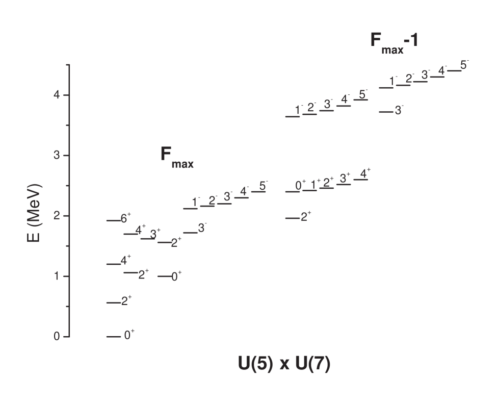
FIG. 2.: Sketch of the relevant low-energy spectrum in the U(5)$\otimes$U(7) dynamical symmetry limit calculated for five bosons ($N_{\pi}=4$, $N_{\nu}=1$) with the set of parameters: $\epsilon_{d}=0.5$ MeV, $\epsilon_{f}=1.6$ MeV, $\gamma=0.01$ MeV, $\lambda=0.4$ MeV and $\lambda^{\prime}=-0.12$ MeV. The other parameters from Eq. (21) are put equal to 0.

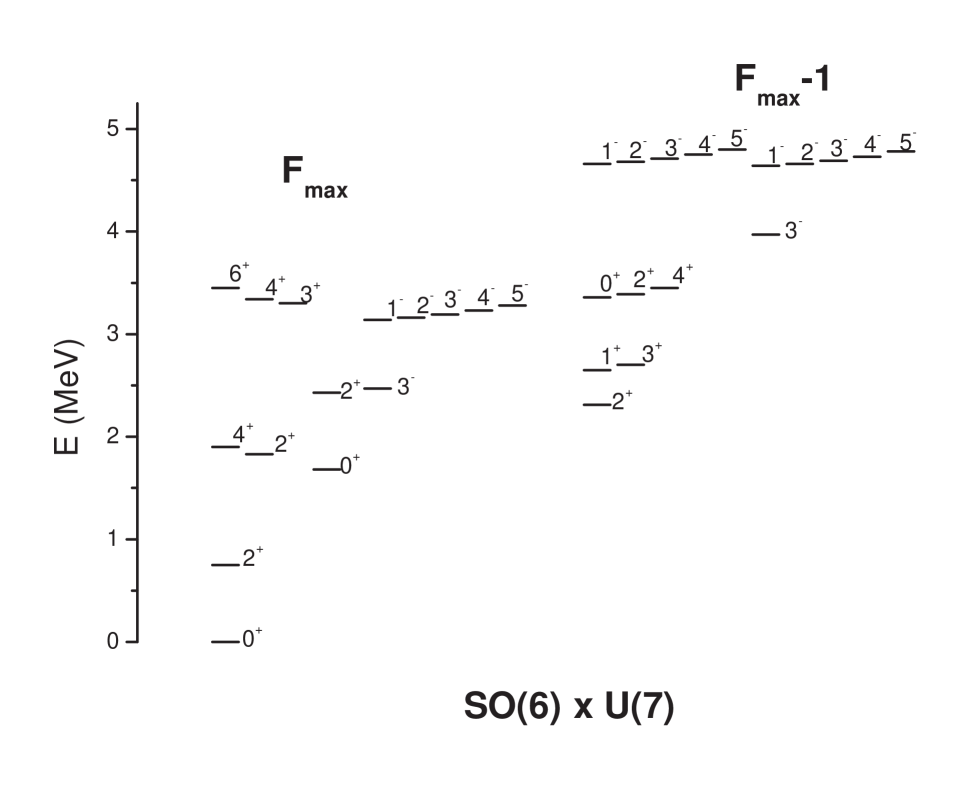
FIG. 3.: Sketch of the relevant low-energy spectrum in the SO(6)$\otimes$U(7) dynamical symmetry limit with the set of parameters: $\zeta=-0.07$ MeV, $\beta=0.18$ MeV, $\epsilon_{f}=1.5$ MeV, $\gamma=0.005$ MeV, $\lambda=0.3$ MeV, $\lambda^{\prime}=-0.1$ MeV and $H_{0}=3.15$ MeV (the other parameters from (25) are equal to 0) and $N_{\pi}=4$, $N_{\nu}=1$.

REFERENCES

- [1] A. Bohr and B. R. Mottelson, Nuclear Structure II (Benjamin, New York, 1975).
- [2] A. Aprahamian, D.S. Brenner, R.F. Casten, R.L. Gill and A. Pietrowski, Phys. Rev. Lett. 59 (1987) 535.
- [3] J. Kern, P.E. Garrett, J. Jolie and H. Lehmann, Nucl. Phys. A 593 (1995) 21.
- [4] R.F. Casten, J. Jolie, H.G. Börner, D.S. Brenner, N.V. Zamfir, W.-T. Chou and A. Aprahamian, Phys. Lett. B 297 (1992) 19; Phys. Lett. B 300 (1993) 411.
- [5] R. Schmidt, Th. Blaich, Th.W. Elze, H. Emling, H. Freiesleben, K. Grimm, W. Henning, R. Holzmann, J.G. Keller, H. Klingler, R. Kulessa, J.V. Kratz, D. Lambrecht, J.S. Lange, Y. Leifels, E. Lubkiewicz, E.F. Moore, E. Wajda, W. Prokopowicz, Ch. Schutter, H. Spies, K. Stelzer, J. Stroth, and W. Walus, H.J. Wollersheim, M. Zinser and E. Zude, Phys. Rev. Lett. 70 (1993) 1767.
- [6] T. Aumann, P.F. Bortignon and H. Emling, Ann. Rev. Nucl. Part. Sci. 48 (1998) 351.
- [7] C. Volpe, Ph. Chomaz, M.V. Andres, F. Catara and E.G. Lanza, Nucl. Phys. A 647 (1999) 246.
- [8] P. Kleinheinz, J. Styczen, M. Piiparinen, J. Blomqvist and M. Kortelahti, Phys. Rev. Lett. 48 (1982) 1457.
- [9] M. Yeh, P.E. Garrett, C.A. McGrath, S.W. Yates and T. Belgya, Phys. Rev. Lett. 76 (1996) 1208.
- [10] H.G. Börner, J. Jolie, S.J. Robinson, B. Krusche, R. Piepenbring, R.F. Casten, A. Aprahamian and J.P. Draayer, Phys. Rev. Lett. 66 (1991) 691.
- [11] P.E. Garrett, M. Kadi, M. Li, C.A. McGrath, V. Sorokin, M. Yeh and S.W. Yates, Phys. Rev. Lett. 78 (1997) 4545.
- [12] P. O. Lipas, Nucl. Phys. 82 (1966) 91.
- [13] P. Vogel and L. Kocbach, Nucl. Phys. A 176 (1971) 33.
- [14] R. A. Gatenby, J. R. Vanhoy, E. M. Baum, E.L. Johnson, S.W. Yates, T. Belgya, B. Fazekas, A. Veres and G. Molnar, Phys. Rev. C 41 (1990) R414.
- [15] S. J. Robinson, J. Jolie, H. G. Börner, P. Schillebeeckx, S. Ulbig and K.P. Lieb, Phys. Rev. Lett. 73 (1994) 412.
- [16] S. F. Hicks, C. M. Davoren, W. M. Faulkner and J. R. Vanhoy, Phys. Rev. C 57 (1998) 2264.
- [17] J. R. Vanhoy, J. M. Anthony, B. M. Haas, B.H. Benedict, B.T. Meehan, S.F. Hicks, C.M. Davoren and C.L. Lundstedt, Phys. Rev. C 52 (1995) 2387.
- [18] P. E. Garrett, H. Lehmann, J. Jolie, C.A. McGrath, M. Yeh and S.W. Yates, Phys. Rev. C 59 (1999) 2455.
- [19] L. Esser, R.V. Jolos and P. von Brentano, Nucl. Phys. A 650 (1999) 157.
- [20] F.R. Metzger, Phys. Rev. C 17 (1978) 939.
- [21] R.-D. Herzberg, I. Bauske, P. von Brentano, Th. Eckert, R. Fischer, W. Geiger, U. Kneissl, J. Margraf, H. Maser, N. Pietralla, H.H. Pitz and A. Zilges, Nucl. Phys. A 592 (1995) 211.
- [22] J. Bryssinck, L. Govor, D. Belic, F. Bauwens, O. Beck, P. von Brentano, D. De Frenne, T. Eckert, C. Fransen, K. Govaert, R.-D. Herzberg, E. Jacobs, U. Kneissl, H. Maser, A. Nord, N. Pietralla, H.H. Pitz, V.Yu. Ponomarev and V. Werner, Phys. Rev. C 59 (1999) 1930.
- [23] M. Wilhelm, E. Radermacher, A. Zilges and P. von Brentano, Phys. Rev. C 54 (1996) R449.
- [24] M. Wilhelm, S. Kasemann, G. Pascovici, E. Radermacher, P. von Brentano, and A. Zilges, Phys. Rev. C 57 (1998) 577.
- [25] U. Kneissl, H. H. Pitz and A. Zilges, Prog. Part. Nucl. Phys. 37 (1996) 349.
- [26] Norbert Pietralla, Phys. Rev. C 59 (1999) 2941.
- [27] W. D. Hamilton, A. Irbäck and J. P. Elliott, Phys. Rev. Lett. 53 (1984) 2469.
- [28] W. J. Vermeer, C. S. Lim and R. H. Spear, Phys. Rev. C 38 (1998) 2982.
- [29] B. Fazekas, T. Belgya, G. Molnar, A. Veres, R.A. Gatenby, S.W. Yates and T. Otsuka, Nucl. Phys. A 548 (1992) 249.
- [30] P.E. Garrett, H. Lehmann, C.A. McGrath, Minfang Yeh and S.W. Yates, Phys. Rev. C 54 (1996) 2259.
- [31] I. Wiedenhöver, A. Gelberg, T. Otsuka, N. Pietralla, J. Gableske, A. Dewald and P. von Brentano, Phys. Rev. C 56 (1997) R2354.
- [32] N. Pietralla, D. Belic, P. von Brentano, C. Fransen, R.-D. Herzberg, U. Kneissl, H. Maser, P. Matschinsky, A. Nord, T. Otsuka, H.H. Pitz, V. Werner and I. Wiedenhöver, Phys. Rev. C 58 (1998) 796.
- [33] N. Pietralla, C. Fransen, D. Belic, P. von Brentano, C. Friessner, U. Kneissl, A. Linnemann, A. Nord, H. H. Pitz, T. Otsuka, I. Schneider, V. Werner and I. Wiedenhöver, Phys. Rev. Lett. 83 (1999) 1303.
- [34] A. Arima, T. Otsuka, F. Iachello and I. Talmi, Phys. Lett. B 66 (1977) 205.
- [35] T. Otsuka, Ph.D. thesis, University of Tokyo, 1978, unpublished.
- [36] F. Iachello, Phys. Rev. Lett. 53 (1984) 1427.
- [37] N. Pietralla, C. Fransen, P. von Brentano, C. Frießner, A. Gade, A. Linnemann, P. Matschinsky, I. Schneider, V. Werner, I. Wiedenhöver, D. Belic, U. Kneissl, A. Nord and H. H. Pitz, Contribution to the International Conference on Nuclear Models 1998, October, 12 – 14 1998, Camerino, Italy, in press.
- [38] N. Pietralla, C. Fransen, A. Dewald, C. Frießner, J. Gableske, P. von Brentano, Phys. Rev. Lett. 84, (2000) 3775.
- [39] C. Fransen et al., in preparation.
- [40] A. Arima and F. Iachello, Phys. Rev. Lett. 35 (1975) 1069.
- [41] F. Iachello and A. Arima, The Interacting Boson Model (Cambridge University Press, Cambridge, 1987).
- [42] C. S. Han, D. S. Chuu, S. T. Hsieh and H. C. Chiang, Phys. Lett. B 163 (1988) 295.
- [43] A. F. Barfield, P. von Brentano, A. Dewald, K. O. Zell, N. V. Zamfir, D. Bucurescu, M. Ivascu and O. Scholten, Z. Phys. A 332 (1989) 29.
- [44] G. Racah, Phys. Rev. 76 (1949) 1352.
- [45] S. G. Rohozińsky, J. Phys. G 4 (1978) 1075.
- [46] B. G. Wybourne, Symmetry Principles and Atomic Spectroscopy (Wiley-Interscience, New York, 1970)
- [47] G. Maino, A. Ventura, L. Zuffi and F. Iachello, Phys. Lett. B 152 (1985) 17.
- [48] J. Engel and F. Iachello, Nucl. Phys. A 472 (1987) 61.
- [49] T. Otsuka and M. Sugita, Phys. Lett. B 209 (1988) 140.
- [50] D. F. Kusnezov and F. Iachello, Phys. Lett. B 209 (1988) 420.
- [51] M. Sugita, T. Otsuka and P. von Brentano, Phys. Lett. B 389 (1996) 642.
- [52] G. L. Long, T. Y. Shen, H. Y. Ji and E. G. Zhao, Phys. Rev. C 57 (1998) 2301.
- [53] R.-D. Herzberg, P. von Brentano, J. Eberth, J. Enders, R. Fischer, N. Huxel, T. Klemme. P. Von Neumann-Cosel, N. Nicolay, N. Pietralla, V. Yu. Ponomariev, J. Reif, A. Richter, C. Schlegel, R. Schwengner, S. Skoda, H. G. Thomas, I. Wiedenhöver and A. Zilges, Phys. Lett. B 390 (1997) 49.
- [54] V. Yu. Ponomarev, Eur. Phys. J. A 6, 243 (1999) 243.
- [55] P. von Brentano, N. V. Zamfir and A. Zilges, Phys. Lett. B 278 (1992) 221.
- [56] P. Van Isacker, K. Heyde, J. Jolie and A. Sevrin, Ann. Phys. (N.Y.) 171 (1986) 253.
- [57] O. Scholten, Ph.D. thesis (1980).