QCD sum rules for $J/\psi$ in the nuclear medium: calculation of the Wilson coefficients of gluon operators up to dimension 6

Abstract

We calculate the Wilson coefficients of all dimension 6 gluon operators with non zero spin in the correlation function between two heavy vector currents. For the twist-4 part, we first identify the three independent gluon operators, and then proceed with the calculation of the Wilson coefficients using the fixed point gauge. Together with the previous calculation of the Wilson coefficients for the dimension 6 scalar gluon operators by Nikolaev and Radyushkin, our result completes the list of all the Wilson coefficients of dimension 6 gluon operators in the correlation function between heavy vector currents. We apply our results to investigate the mass of $J/\psi$ in nuclear matter using QCD sum rules. Using an upper bound estimate on the matrix elements of the dimension 6 gluon operators to linear order in density, we find that the density dependent contribution from dimension 6 operators is less than $40\%$ of the dimension 4 operators with opposite sign. The final result gives about $-4$ MeV mass shift for the charmonium at rest in nuclear matter.

1 Introduction

Identifying higher twist operators and calculating their corresponding Wilson coefficients are very important in several aspects. First, these provide a systematic building blocks to analyze the available data from deep inelastic scattering(DIS) at lower $Q^{2}$ region. Second, these contributions are essential for a realistic generalization of QCD sum rule methods to finite baryon density.

The twist-4 operators were classified and its anomalous dimensions for some of the operators were calculated by S. Gottlieb[1]. However, the operators were over-determined and the independent set of twist-4 operators appearing in the DIS were first identified by Jaffe and Soldate[2], where the twist-4 operators are of four quark type and quark gluon mixed type. Among the uses of these results, the available DIS data were analyzed to determine the nucleon matrix elements of the twist-4 operators[3, 4]. These estimates were then used in generalizing the QCD sum rule approaches for light vector mesons to finite density[5, 6].

In the correlation function of two heavy vector currents, only gluon operators contribute in the operator product expansion(OPE). This is so because in the heavy quark system, all the heavy quark condensates are generated via gluonic condensates[7, 8, 9]. In dimension 6, there are scalar operators, twist-2 and twist-4 operators. For the scalar gluonic operators at dimension 6, there are two independent operators. In ref.[10], the two were identified and the corresponding Wilson coefficient were calculated . For twist-2 gluon operator, the calculation for the leading order(LO) Wilson coefficient is simple and its matrix element is just the second moment of the gluon structure function.

The twist-4 dimension 6 gluon operators are more involved. In this work, we have identified the three independent local gluon operators and calculated their corresponding LO Wilson coefficients in the correlation function between two heavy vector currents. This result is new and complimentary to a previous work[11] on gluon twist-4 operators, where they start from certain diagrams and identify the three independent twist-4 gluon structure functions. Together with the previous calculation of the Wilson coefficients for the dimension 6 scalar gluon operators by Nikolaev and Radyushkin[10], our result completes the list of all the Wilson coefficients of dimension 6 gluon operators in the correlation function between heavy vector currents. As an application, we will use our result in QCD sum rule approach to investigate the property of $J/\psi$ in nuclear matter.

This is particularly interesting because the on-going discussion of $J/\psi$ suppression in RHIC as a possible signal for quark gluon plasma[12], inevitably requires a detailed knowledge of the changes of $J/\psi$ properties in “normal” nuclear matter[13]. Furthermore, the large charm quark mass $m_{c}\gg\Lambda_{QCD}$ provides a natural renormalization point for which a perturbative QCD expansion is partly possible. In fact, studies have shown that the multi-gluon exchange between a $c\bar{c}$ pair and nucleons might induce a bound $c\bar{c}$ state with even light nuclei[14, 15, 16, 17, 18, 19, 20]. In such analysis, the low energy multi-gluon potential was modeled either from the effective theory obtained in the infinitely large $m_{Q}$ limit[16, 17, 18] or from extrapolating the high energy scattering via pomeron exchange to lower energy[14]. Although both approaches, gave similar binding for the $J/\psi$ in nuclear matter, it is not clear how reliable these results are unless one systematically calculates the corrections.

In order to confirm this findings in an alternative but a systematic approach and to establish a basis for further studies, we have previously applied the QCD sum rules[7, 8] to heavy quark system in nuclear medium and calculated the mass of $J/\psi$ and $\eta_{c}$ in nuclear medium[21, 22]. This was the generalization of the sum rule method for the light vector mesons in medium[5] to the heavy quark system. It was found that the mass of $J/\psi$ ($\eta_{c}$) would reduce by 7 MeV (5 MeV), which is indeed consistent with previous results based on completely different methods[15, 16, 19, 20]. However, it was not possible to reliably estimate the uncertainties of the result, because the contribution from the operator product expansion was truncated at the leading dimension 4 operators. To overcome the limitations , we will here make use of our calculation to include the complete dimension 6 contributions. Unfortunately, at present, there is no data to identify the nucleon expectation value of any of the dimension 6 operators(scalar, twist-2, twist-4) nor is there any lattice result. Nevertheless, in this article, we will estimate the nucleon matrix elements of these operators and then use QCD sum rule approach to study the reliability of our previous result on the mass shift of $J/\psi$ in nuclear matter. If in the future, the matrix elements are better known, we will be able to study the non trivial momentum dependence of the $J/\psi$ in nuclear medium, as has been done for the light vector mesons[6]. The momentum dependence is especially interesting because, there are inelastic channels opening when the charmonium system is moving with respect to the medium. For example, when the charmonium is moving with sufficient velocity, it will have enough energy to interact with a nucleon to produce a D meson and a charmed nucleon. This effect would be very important in relation to $J/\psi$ suppression in RHIC.

In section 2 we characterize all gluon operator up to dimension 6 and obtain identities to be used to reduce the operators to an independent set. In section 3, we calculate the Wilson coefficients for the independent set of gluon operators and show current conservation. In section 4, we calculate the moments and perform a moment sum rules analysis to calculate the $J/\psi$ mass in nuclear matter. We conclude with some discussions. The appendix includes some detailed calculation of the Wilson coefficients.

2 Operators

In the operator product expansion of heavy quark system, only gluonic condensates are relevant. This is so because all the heavy quark condensates can be related to the gluon condensates via heavy quark expansion [7, 8, 9]. This is also true in nuclear medium since there are no valence charm quarks to leading order in density and any interaction with the medium is gluonic. Let us start by categorizing gluonic operators up to dimension 6, which does not vanish in nuclear matter.

For dimension 4 operators, the scalar and twist-2 gluon operators contribute [21, 22],

$$g^{2}G^{a}_{\mu\nu}G^{a}_{\mu\nu},~{}~{}~{}~{}g^{2}G^{a}_{\mu\alpha}G^{a}_{\nu\alpha}.$$ (1)

For dimension 6 operators, one can think of generating a number of gluon operators constructed from three gluon fields $G^{a}_{\mu\nu}$ or two gluon fields with two covariant derivatives. However, for scalar operators, there are only two independent scalar operators[10]. They are,

$$g^{3}f^{abc}G^{a}_{\mu\nu}G^{b}_{\mu\alpha}G^{c}_{\nu\alpha},~{}~{}~{}~{}~{}g^{2}G^{a}_{\mu\alpha}G^{a}_{\nu\alpha;\nu\mu}.$$ (2)

The second operator can also be written in terms of four quark operator using the equation of motion

$$G^{a}_{\mu\nu;\nu}=g\bar{q}\gamma_{\mu}\frac{\lambda^{a}}{2}q=gj_{\mu}^{a},$$ (3)

As for the spin 2 operators in dimension 6, which are also called dimension 6 twist 4 (twist=dimension-spin) operator, we can first categorize possible operators as follows. First, there is again one operator with three gluon field strength tensor. Then, assuming the free symmetric and traceless indices to be $\mu$ and $\nu$, depending on whether or not the free index goes into the covariant derivative, there are 6 more operators possible. Starting with the three gluon operator, the 7 are,

$$g^{3}f^{abc}G^{a}_{\mu\kappa}G^{b}_{\nu\lambda}G^{c}_{\kappa\lambda}\equiv g^{3}fG^{3}_{\mu\nu}$$

$$g^{2}G^{a}_{\kappa\lambda}G^{a}_{\kappa\lambda;\mu\nu}$$

$$g^{2}G^{a}_{\mu\kappa}G^{a}_{\nu\lambda;\kappa\lambda},\,\,g^{2}G^{a}_{\mu\kappa}G^{a}_{\nu\kappa;\lambda\lambda},\,\,g^{2}G^{a}_{\mu\kappa}G^{a}_{\nu\lambda;\lambda\kappa}$$

$$g^{2}G^{a}_{\mu\kappa}G^{a}_{\kappa\lambda;\lambda\nu},\,\,g^{2}G^{a}_{\kappa\lambda}G^{a}_{\mu\kappa;\lambda\nu}.$$ (4)

However, they are not independent. Using the identities in appendix A, one can show that there are three independent spin-2 operators at dimension 6. The set we will use are,

$$g^{2}\,G^{a}_{\kappa\lambda}G^{a}_{\kappa\lambda;\mu\nu},~{}~{}g^{2}\,G^{a}_{\mu\kappa}G^{a}_{\nu\lambda;\lambda\kappa},~{}~{}g^{2}\,G^{a}_{\mu\kappa}G^{a}_{\kappa\lambda;\lambda\nu}.$$ (5)

It is interesting to note that in reference [11] starting from certain diagrams with two, three and four gluon exchange in the t-channel, they were able to derive three twist-4 gluon distribution amplitudes, from which one can calculate the nucleon matrix element of the three independent operators.

As for the spin 4 dimension 6 operator, it is just the twist-2 gluon operator.

3 Polarization (OPE)

Having established the independent gluon operators in dimension 6, we will calculate their LO Wilson coefficients in the correlation function between two vector currents made of heavy quarks, $j_{\mu}={\bar{h}}\gamma_{\mu}h$.

$$\Pi_{\mu\nu}(q) = i\int d^{4}xe^{iqx}\langle{\rm T}\{j_{\mu}(x)j_{\nu}(0)\}\rangle_{\rho}$$ (6)

$$= i\int d^{4}xe^{iqx}\langle{\rm Tr}\left[\gamma_{\mu}S(x,0)\gamma_{\nu}S(0,x))\right]\rangle_{\rho}$$

$$= i\int\frac{d^{4}k}{(2\pi)^{4}}\langle\,{\rm Tr}[\,\gamma_{\mu}S(k+q)\gamma_{\nu}{\tilde{S}}(k)]\,\rangle_{\rho},$$

where $\langle\cdot\rangle_{\rho}$ represents the expectation value at finite nuclear density $\rho$. The fourier transforms are defined by

$$iS(p)=\int d^{4}xe^{ipx}\,iS(x,0)$$

$$i{\tilde{S}}(p)=\int d^{4}xe^{-ipx}\,iS(0,x).$$ (7)

$S(x,0)$ is the heavy quark propagator in the presence of external gluon field [23]. To calculate the Wilson coefficients, we obtain the quark propagator in the presence of external gauge fields in the Fock-Schwinger gauge [10, 23],

$$x_{\mu}A^{a}_{\mu}(x)=0.$$ (8)

In appendix C we list the momentum space representation of the quark propagator multiplying the gauge invariant gluon operators. We will use these quark propagators in eq.(6) and extract the Wilson coefficients by collecting the appropriate tensor and gluon structures.

In general the polarization tensor in eq.(6) will have two invariant functions. They can be divided into the longitudinal and transverse part of the external three momentum, which are the following when the nuclear matter is at rest.

$$\Pi_{L}=\frac{1}{k^{2}}\Pi_{00},~{}~{}~{}~{}\Pi_{T}=-\frac{1}{2}(\frac{1}{q^{2}}\Pi^{\mu}_{\mu}+\frac{1}{k^{2}}\Pi_{00}),$$ (9)

where $q=(\omega,k)$ is the external momentum.

In the vacuum or in the limit when $k\rightarrow 0$ they become the same so that there is only one invariant function

$$\Pi_{L}(\omega^{2})=\Pi_{T}(\omega^{2})=\frac{-1}{3\omega^{2}}g^{\mu\nu}\Pi_{\mu\nu}\equiv\Pi(\omega^{2}).$$ (10)

So in this work, we will construct the sum rule for $\Pi(\omega^{2})$ at $k\rightarrow 0$ and nuclear matter at rest. However, in the calculation of the OPE, we will start from the general expression of eq.(6) at nonzero value of $k$ and calculate each tensor structure separately. This way, current conservation will be a nontrivial check of our calculation and the generalization to $k\neq 0$ will be straightforward[24].

In the following subsections, we will summarize the OPE for operators of dimension 4 and 6. The new results of the present work are the OPE for dimension 6 spin 2 and dimension 6 spin 4 operators.

3.1 scalar contributions

Here we summarize the OPE of scalar operators of dimension 4 and dimension 6 used in the vacuum sum rule[10].

$$\Pi^{\rm scalar}_{\mu\nu}(q) = (q_{\mu}q_{\nu}-g_{\mu\nu}q^{2})\Big{[}C^{pert.}+C^{0}_{G^{2}}\langle g^{2}G^{a}_{\alpha\beta}G^{a}_{\alpha\beta}\rangle$$ (11)

$$+C^{0}_{G^{3}}\langle g^{3}f^{abc}G^{a}_{\alpha\beta}G^{b}_{\beta\lambda}G^{c}_{\lambda\alpha}\rangle+C^{0}_{j^{2}}\langle g^{4}j^{a}_{\kappa}j^{a}_{\kappa}\rangle\Big{]},$$

where

$$C^{0}_{G^{2}}=\frac{1}{48\pi^{2}(Q^{2})^{2}}[-1+3J_{2}-2J_{3}],$$

$$C^{0}_{G^{3}}=\frac{1}{72\pi^{2}(Q^{2})^{3}}\left[\frac{2}{15}-\frac{1}{10}y+4J_{2}-\frac{31}{3}J_{3}+\frac{43}{5}J_{4}-\frac{12}{5}J_{5}\right],$$

$$C^{0}_{j^{2}}=\frac{1}{36\pi^{2}(Q^{2})^{3}}\left[\frac{41}{45}-\frac{3}{5}y+(\frac{2}{3}+\frac{1}{3}y)J_{1}-J_{2}-\frac{4}{9}J_{3}-\frac{26}{15}J_{4}+\frac{8}{5}J_{5}\right],$$ (12)

and

$$J_{N}(y)=\int^{1}_{0}\frac{dx}{\left[1+x(1-x)y\right]^{N}},$$ (13)

with $y=Q^{2}/m^{2}$ and $m$ being the heavy quark mass. This will give the following contribution to $\Pi(\omega^{2})$ defined in eq.(10).

$$\Pi(\omega^{2}) = C^{pert.}+C^{0}_{G^{2}}\langle g^{2}G^{a}_{\alpha\beta}G^{a}_{\alpha\beta}\rangle+C^{0}_{G^{3}}\langle g^{3}f^{abc}G^{a}_{\alpha\beta}G^{b}_{\beta\lambda}G^{c}_{\lambda\alpha}\rangle$$ (14)

$$+C^{0}_{j^{2}}\langle g^{4}j^{a}_{\kappa}j^{a}_{\kappa}\rangle.$$

For later convenience, we will use $g^{3}f^{abc}G^{a}_{\mu\nu}G^{b}_{\nu\lambda}G^{c}_{\lambda\mu}=\frac{1}{2}g^{2}G^{a}_{\mu\nu}G^{a}_{\mu\nu;\alpha\alpha}+g^{4}j^{a}_{\mu}j^{a}_{\mu}$ and rewrite the OPE as follows,

$$\Pi(\omega^{2}) = C^{pert.}+C_{G^{2}}\langle\frac{\alpha_{s}}{\pi}G^{a}_{\mu\nu}G^{a}_{\mu\nu}\rangle+C_{GD^{2}G}\langle\frac{\alpha_{s}}{\pi}G^{a}_{\mu\nu}G^{a}_{\mu\nu;\kappa\kappa}\rangle$$ (15)

$$+C_{j^{2}}\cdot\frac{2}{3}\langle\frac{\alpha_{s}}{\pi}G^{a}_{\alpha\kappa}G^{a}_{\alpha\lambda;\lambda\kappa}\rangle,$$

where

$$C_{G^{2}} = \frac{1}{12(Q^{2})^{2}}[-1+3J_{2}-2J_{3}],$$

$$C_{GD^{2}G} = \frac{1}{1080(Q^{2})^{3}}[4-3y+120J_{2}-310J_{3}+258J_{4}-72J_{5}],$$

$$C_{j^{2}} = \frac{1}{1080(Q^{2})^{3}}[(4-3y+120J_{2}-310J_{3}+258J_{4}-72J_{5})$$ (16)

$$-180+120y-(120+60y)J_{1}-300J_{2}+1320J_{3}-720J_{4}].$$

Note $Q^{2}=-\omega^{2}$ in our kinematical limit.

3.2 dimension 4 spin 2 operator

This part has been calculated recently [21, 22]. Here we summarize the results.

$$\Pi^{4,2}_{\mu\nu}(q) = \frac{1}{Q^{2}}\bigg{[}{\cal I}^{2}_{\mu\nu}+\frac{1}{Q^{2}}(q_{\rho}q_{\mu}{\cal I}^{2}_{\rho\nu}+q_{\rho}q_{\nu}{\cal I}^{2}_{\rho\mu})$$ (17)

$$+g_{\mu\nu}\frac{q_{\rho}q_{\sigma}}{Q^{2}}{\cal J}^{2}_{\rho\sigma}+\frac{q_{\mu}q_{\nu}q_{\rho}q_{\sigma}}{Q^{4}}({\cal I}^{2}_{\rho\sigma}+{\cal J}^{2}_{\rho\sigma})\bigg{]},$$

where

$${\cal I}^{2}_{\mu\nu} = \langle\frac{\alpha_{s}}{\pi}G^{a}_{\sigma\mu}G^{a}_{\sigma\nu}\rangle\left[\frac{1}{2}+(1-\frac{1}{3}y)J_{1}-\frac{3}{2}J_{2}\right]$$

$${\cal J}^{2}_{\mu\nu} = \langle\frac{\alpha_{s}}{\pi}G^{a}_{\sigma\mu}G^{a}_{\sigma\nu}\rangle\left[-\frac{7}{6}+(1+\frac{1}{3}y)J_{1}-\frac{1}{2}J_{2}+\frac{2}{3}J_{3}\right].$$ (18)

3.3 contribution from dimension 6 and spin 4

The diagrams describing interactions with the gluonic field in dimension 6 are shown in Fig 1.

The calculation for this part is straightforward. We substitute into eq.(6) parts of the quark propagator containing $D$’s and $G$’s (summarized in appendix C) so that when these from the two propagators are combined, yield terms proportional to $GDDG$. In Fig.1, these come from Fig.1(c) to Fig.1(g). Then we extract the traceless and symmetric spin-4 part of the operator $GDDG$. The final result for the dimension 6 spin 4 part of the operators yields,

$$\Pi^{6,4}_{\mu\nu}(q) = \frac{q_{\kappa}q_{\lambda}}{(Q^{2})^{3}}\bigg{[}I^{4}_{\kappa\lambda\mu\nu}+\frac{1}{Q^{2}}(q_{\rho}q_{\mu}I^{4}_{\kappa\lambda\rho\nu}+q_{\rho}q_{\nu}I^{4}_{\kappa\lambda\rho\mu})$$ (19)

$$+g_{\mu\nu}\frac{q_{\rho}q_{\sigma}}{Q^{2}}J^{4}_{\kappa\lambda\rho\sigma}+\frac{q_{\mu}q_{\nu}q_{\rho}q_{\sigma}}{Q^{4}}(I^{4}_{\kappa\lambda\rho\sigma}+J^{4}_{\kappa\lambda\rho\sigma})\bigg{]},$$

where

$$I^{4}_{\mu\nu\rho\sigma} = \left[-\frac{266}{45}+\left(-\frac{20}{3}+\frac{22}{15}y\right)J_{1}+\frac{138}{5}J_{2}-\frac{916}{45}J_{3}+\frac{16}{3}J_{4}\right]$$

$$\times\langle\frac{\alpha_{s}}{\pi}G^{a}_{\rho\kappa}G^{a}_{\sigma\kappa;\mu\nu}\rangle$$

$$J^{4}_{\mu\nu\rho\sigma} = \left[\frac{362}{45}-\left(4+\frac{22}{15}y\right)J_{1}-\frac{94}{15}J_{2}-\frac{44}{45}J_{3}+\frac{16}{3}J_{4}-\frac{32}{15}J_{5}\right]$$ (20)

$$\times\langle\frac{\alpha_{s}}{\pi}G^{a}_{\rho\kappa}G^{a}_{\sigma\kappa;\mu\nu}\rangle.$$

Figure 1: 1-loop diagrams describing interactions with the gluonic field giving dimension 6 operators: The dashed line represents an external gluon field $G$ and the dashed line with $n$ arrows represents an external gluon field with $n$ derivatives $D^{n}G$.

3.4 contributions from dimension 6 and spin 2

The calculation for this part goes in a similar way as in the previous subsection. However, this time all the graphs in Fig.1 contribute. Moreover, we have to include all possible combination of $G$ and $D$’s that makes up dimension 6. We then extract the spin 2 part of each operator and use the identities given in the appendix to reduce the operators into the independent three in eq.(5). An example needed to extract the spin 2 part from a general operator is given in appendix D. Finally we find,

$$\Pi^{6,2}_{\mu\nu}(q) = \frac{1}{(Q^{2})^{2}}\bigg{[}I^{2}_{\mu\nu}+\frac{1}{Q^{2}}(q_{\rho}q_{\mu}I^{2}_{\rho\nu}+q_{\rho}q_{\nu}I^{2}_{\rho\mu})$$ (21)

$$+g_{\mu\nu}\frac{q_{\rho}q_{\sigma}}{Q^{2}}J^{2}_{\rho\sigma}+\frac{q_{\mu}q_{\nu}q_{\rho}q_{\sigma}}{Q^{4}}(I^{2}_{\rho\sigma}+J^{2}_{\rho\sigma})\bigg{]},$$

where

$$I^{2}_{\mu\nu} = \langle\frac{\alpha_{s}}{\pi}G^{a}_{\kappa\lambda}G^{a}_{\kappa\lambda;\mu\nu}\rangle\left[\frac{31}{240}-\frac{1}{60}y+\left(\frac{13}{24}+\frac{1}{48}y\right)J_{1}-\frac{115}{48}J_{2}+\frac{21}{8}J_{3}-\frac{9}{10}J_{4}\right]$$

$$+\langle\frac{\alpha_{s}}{\pi}G^{a}_{\mu\kappa}G^{a}_{\nu\lambda;\lambda\kappa}\rangle\left[-\frac{739}{720}+\frac{2}{15}y+\left(-\frac{9}{8}+\frac{3}{16}y\right)J_{1}+\frac{133}{48}J_{2}+\frac{1}{72}J_{3}-\frac{19}{30}J_{4}\right]$$

$$+\langle\frac{\alpha_{s}}{\pi}G^{a}_{\mu\kappa}G^{a}_{\kappa\lambda;\lambda\nu}\rangle\left[\frac{293}{240}-\frac{3}{10}y+\left(\frac{55}{24}+\frac{1}{16}y\right)J_{1}-\frac{131}{16}J_{2}+\frac{145}{24}J_{3}-\frac{41}{30}J_{4}\right]$$

$$J^{2}_{\mu\nu} = \langle\frac{\alpha_{s}}{\pi}G^{a}_{\kappa\lambda}G^{a}_{\kappa\lambda;\mu\nu}\rangle\left[\frac{103}{240}+\frac{1}{60}y+\left(\frac{5}{24}-\frac{7}{48}y\right)J_{1}-\frac{59}{48}J_{2}+\frac{31}{24}J_{3}-\frac{11}{10}J_{4}+\frac{2}{5}J_{5}\right]$$ (22)

$$+\langle\frac{\alpha_{s}}{\pi}G^{a}_{\mu\kappa}G^{a}_{\nu\lambda;\lambda\kappa}\rangle\left[\frac{71}{240}-\frac{2}{15}y+\left(-\frac{1}{8}+\frac{1}{48}y\right)J_{1}+\frac{61}{48}J_{2}-\frac{61}{24}J_{3}+\frac{29}{30}J_{4}+\frac{2}{15}J_{5}\right]$$

$$+\langle\frac{\alpha_{s}}{\pi}G^{a}_{\mu\kappa}G^{a}_{\kappa\lambda;\lambda\nu}\rangle\left[\frac{29}{240}+\frac{3}{10}y-\left(\frac{1}{24}+\frac{7}{16}y\right)J_{1}+\frac{31}{48}J_{2}-\frac{23}{24}J_{3}+\frac{11}{30}J_{4}-\frac{2}{15}J_{5}\right].$$

There are few checks we can perform to verify our calculation. First, although the polarization function in eq.(6) has only two invariant parts, we performed the calculation directly leaving the indices $\mu,\nu$ free. This means that we have obtained and calculated the 6 different possible tensor structure, given in appendix B, separately. Therefore, showing current conservation, $q^{\mu}\Pi_{\mu\nu}=q^{\nu}\Pi_{\mu\nu}=0$ is a non-trivial check. Another indirect check is that the final result is regular at $Q^{2}=0$. That is, making a small $Q^{2}$ expansion one can show that all the Wilson coefficients in eq.(3.2), eq.(3.3) and eq.(3.4) are regular.

Eq.(11), eq.(17), eq.(19) and eq.(21) form the complete OPE up to dimension 6 operators. Since QCD is renormalizable, there are no other power correction up to this dimension and the Wilson coefficients will be an asymptotic expansion in $1/\log Q^{2}$. In the vacuum, only scalar operators will contribute. However, in medium or when the expectation value is with respect to a nucleon state, the tensor operators will also contribute. As an application of our result, we will apply our OPE to the QCD sum rule analysis for the $J/\psi$ in nuclear matter.

3.5 sum of tensor parts

As we discussed before we will take the nuclear matter to be at rest. Moreover, we will use linear density approximation to evaluate the matrix elements,

$$\langle\cdot\rangle_{\rho}=\langle\cdot\rangle_{0}+\frac{\rho}{2m_{N}}\langle N|\cdot|N\rangle$$ (23)

where $\langle\cdot\rangle_{0}$ is the vacuum expectation value, $\rho$ is the nuclear density, $m_{N}$ the nucleon mass, and the nucleon state $|N\rangle$ is normalized as $\langle N|N\rangle=(2\pi)^{3}2\omega_{N}\delta^{3}(0)$. Then, the OPE from dimension 4 and dimension 6 operators in eq.(17), eq.(19) and eq.(21) give the following contribution to $\Pi$.

$$\Pi(\omega^{2}) = \Pi_{4,2}(\omega^{2})+\Pi_{6,2}(\omega^{2})+\Pi_{6,4}(\omega^{2})$$ (24)

$$= \frac{\rho}{2m_{N}}\left[C_{G_{2}}G_{2}+(C_{X}X+C_{Y}Y+C_{Z}Z)+C_{G_{4}}G_{4}\right],$$

where

$$C_{G_{2}} = \frac{m_{N}^{2}}{12(Q^{2})^{2}}[9-(12+2y)J_{1}+9J_{2}-6J_{3}],$$

$$C_{X} = \frac{m_{N}^{2}}{240(Q^{2})^{3}}[-85-2y+(-70+25y)J_{1}+365J_{2}-390J_{3}+252J_{4}-72J_{5}],$$

$$C_{Y} = \frac{m_{N}^{2}}{720(Q^{2})^{3}}[25+48y+(270-45y)J_{1}-1185J_{2}+1370J_{3}-408J_{4}-72J_{5}],$$

$$C_{Z} = \frac{m_{N}^{2}}{240(Q^{2})^{3}}[-95-36y+(-130+75y)J_{1}+375J_{2}-190J_{3}+16J_{4}+24J_{5}],$$

$$C_{G_{4}} = \frac{m_{N}^{4}}{108(Q^{2})^{3}}[205-(210+33y)J_{1}+99J_{2}-262J_{3}+240J_{4}-72J_{5}],$$ (25)

where again in our kinematical limit $Q^{2}=-\omega^{2}$ and the scalar parts of the matrix elements in nuclear matter to leading density come from the following nucleon expectation values,

$$\langle N|\frac{\alpha_{s}}{\pi}G^{a}_{\sigma\mu}G^{a}_{\sigma\nu}|N\rangle = G_{2}\,(p_{\mu}p_{\nu}-\frac{1}{4}m_{N}^{2}g_{\mu\nu}),$$

$$\langle N|\frac{\alpha_{s}}{\pi}G^{a}_{\kappa\lambda}G^{a}_{\kappa\lambda;\mu\nu}|N\rangle = X\,(p_{\mu}p_{\nu}-\frac{1}{4}m_{N}^{2}g_{\mu\nu}),$$

$$\langle N|\frac{\alpha_{s}}{\pi}G^{a}_{\mu\kappa}G^{a}_{\nu\lambda;\lambda\kappa}|N\rangle = Y\,(p_{\mu}p_{\nu}-\frac{1}{4}m_{N}^{2}g_{\mu\nu}),$$

$$\langle N|\frac{\alpha_{s}}{\pi}G^{a}_{\mu\kappa}G^{a}_{\kappa\lambda;\lambda\nu}|N\rangle = Z\,(p_{\mu}p_{\nu}-\frac{1}{4}m_{N}^{2}g_{\mu\nu}),$$

$$\langle N|\frac{\alpha_{s}}{\pi}G^{a}_{\mu\kappa}G^{a}_{\nu\kappa;\alpha\beta}|N\rangle = G_{4}\,\bigg{[}p_{\mu}p_{\nu}p_{\alpha}p_{\beta}+\frac{m_{N}^{4}}{48}(g_{\mu\nu}g_{\alpha\beta}+g_{\mu\alpha}g_{\nu\beta}+g_{\mu\beta}g_{\nu\alpha})$$

$$-\frac{1}{8}m_{N}^{2}(p_{\mu}p_{\nu}g_{\alpha\beta}+p_{\mu}p_{\alpha}g_{\nu\beta}+p_{\mu}p_{\beta}g_{\alpha\nu}$$

$$+p_{\nu}p_{\alpha}g_{\mu\beta}+p_{\nu}p_{\beta}g_{\mu\alpha}+p_{\alpha}p_{\beta}g_{\mu\nu})\bigg{]}.$$

Note that here we chose the nucleon four momentum to be $p=(m_{N},0,0,0)$. We discuss the magnitudes of these nucleon matrix elements in section 4.

4 Moment sum rule for $J/\psi$ at rest

4.1 moments

As an application of our result, we will use our result to refine our previous work to calculate the mass shift of the $J/\psi$ in nuclear medium[21] using the moment sum rule [7, 25]. The moments of the polarization function is defined as,

$$M_{n}(Q_{0}^{2})=\frac{1}{n!}\left(-\frac{d}{dQ^{2}}\right)^{n}\Pi(Q^{2})|_{Q^{2}=Q_{0}^{2}}.$$ (27)

where in our kinematics, $Q^{2}=-\omega^{2}$. Direct evaluation of these moments using the OPE gives, up to dimension 4 [25, 21],

$$M_{n}(\xi)=A_{n}^{V}(\xi)\left[1+a_{n}(\xi)\alpha_{s}+b_{n}(\xi)\phi^{4}_{b}+c_{n}(\xi)\phi^{4}_{c}\right],$$ (28)

where

$$\phi^{4}_{b} = \frac{4\pi^{2}}{9}\frac{\langle\frac{\alpha_{s}}{\pi}G^{2}\rangle}{(4m_{c}^{2})^{2}}$$

$$\phi^{4}_{c} = \frac{2\pi^{2}}{3}\frac{G_{2}}{(4m_{c}^{2})^{2}}m_{N}\rho_{N}$$ (29)

and

$$A_{n}^{V}(\xi) = \frac{3}{4\pi^{2}}\frac{2^{n}(n+1)(n-1)!}{(2n+3)!!}(4m^{2})^{-n}(1+\xi)^{-n}\,_{2}F_{1}(n,\frac{1}{2},n+\frac{5}{2};\rho)$$

$$b_{n}(\xi) = -\frac{n(n+1)(n+2)(n+3)}{2n+5}(1+\xi)^{-2}\frac{{}_{2}F_{1}(n+2,-\frac{1}{2},n+\frac{7}{2};\rho)}{{}_{2}F_{1}(n,\frac{1}{2},n+\frac{5}{2};\rho)}$$

$$c_{n}(\xi) = b_{n}(\xi)-\frac{4n(n+1)}{3(2n+5)(1+\xi)^{2}}\frac{{}_{2}F_{1}(n+1,\frac{3}{2},n+\frac{7}{2};\rho)}{{}_{2}F_{1}(n,\frac{1}{2},n+\frac{5}{2};\rho)}$$ (30)

with $\xi=\frac{Q_{0}^{2}}{4m_{c}^{2}}$ and $\rho=\frac{\xi}{1+\xi}$. The factors multiplying the condensate in $\phi^{4}_{b}$ and $\phi^{4}_{c}$ in eq.(4.1) are defined such that at $n\rightarrow\infty~{}$ $c_{n}\sim b_{n}$. Moreover, at this limit, one notes that the contribution from dimension 4 is proportional to $\phi_{b}^{4}+\phi_{c}^{4}$, which in our kinematical limit originates from the following operator form.

$$\phi_{b}^{4}+\phi_{c}^{4}=\frac{16\pi^{2}}{9}{\langle\frac{\alpha}{\pi}G^{a}_{k0}G^{a}_{k0}\rangle\over(4m_{c}^{2})^{2}},$$ (31)

where the operator does not have the trace part of the $00$ index. That is, the leading mass shift is proportional to the color electric field squared $E^{2}$ and the effect coming from the magnetic field squared $B^{2}$ disappears. This is consistent with the non-relativistic picture at the infinite quark mass limit[16], where the Zeeman effect is higher order in $\alpha_{s}$ compared to the Stark effect.

The dimension 6 operators contribute to the moment as follows,

$$\Delta M^{6}_{n}(\xi) = A_{n}^{V}(\xi)\Big{[}\,s_{n}(\xi)\phi^{6}_{s}+t_{n}(\xi)\phi^{6}_{t}+x_{n}(\xi)\phi^{6}_{x}$$ (32)

$$+y_{n}(\xi)\phi^{6}_{y}+z_{n}(\xi)\phi^{6}_{z}+g_{4n}(\xi)\phi^{6}_{g_{4}}\Big{]},$$

where

$$\phi^{6}_{s} = \frac{4\pi^{2}}{3\cdot 1080}\frac{\langle\frac{\alpha_{s}}{\pi}G^{a}_{\mu\nu}G^{a}_{\mu\nu;\kappa\kappa}\rangle}{(4m_{c}^{2})^{3}}$$

$$\phi^{6}_{t} = \left(\frac{2}{3}\right)\frac{4\pi^{2}}{3\cdot 1080}\frac{\langle\frac{\alpha_{s}}{\pi}G^{a}_{\alpha\kappa}G^{a}_{\alpha\lambda;\lambda\kappa}\rangle}{(4m_{c}^{2})^{3}},$$ (33)

come from the scalar operators and

$$\phi^{6}_{x} = \left(\frac{9m_{N}^{2}}{2}\right)\frac{4\pi^{2}}{3\cdot 1080}\frac{X}{(4m_{c}^{2})^{3}}\frac{\rho}{2m_{N}}$$

$$\phi^{6}_{y} = \left(\frac{3m_{N}^{2}}{2}\right)\frac{4\pi^{2}}{3\cdot 1080}\frac{Y}{(4m_{c}^{2})^{3}}\frac{\rho}{2m_{N}}$$

$$\phi^{6}_{z} = \left(\frac{3m_{N}^{2}}{2}\right)\frac{4\pi^{2}}{3\cdot 1080}\frac{Z}{(4m_{c}^{2})^{3}}\frac{\rho}{2m_{N}}$$

$$\phi^{6}_{g_{4}} = (10m_{N}^{4})\frac{4\pi^{2}}{3\cdot 1080}\frac{G_{4}}{(4m_{c}^{2})^{3}}\frac{\rho}{2m_{N}},$$ (34)

are from tensor operators. Note here again that we have put in the prefactors in eq.(33) and eq.(34) such that in the large $n$ limit, all the Wilson coefficients become the same. Specifically, the Wilson coefficients are,

$$s_{n}(\xi) = \sigma_{n}(\xi)f_{n}(0,0;120,-310,258,-72)$$

$$t_{n}(\xi) = s_{n}(\xi)+\sigma_{n}(\xi)f_{n}(-120,-60;-300,1320,-720)$$

$$x_{n}(\xi) = s_{n}(\xi)+\sigma_{n}(\xi)f_{n}(-70,25;245,-80,-6)$$

$$y_{n}(\xi) = s_{n}(\xi)+\sigma_{n}(\xi)f_{n}(270,-45;-1305,1680,-666)$$

$$z_{n}(\xi) = s_{n}(\xi)+\sigma_{n}(\xi)f_{n}(390,-225;-1245,880,-306)$$

$$g_{4n}(\xi) = s_{n}(\xi)+\sigma_{n}(\xi)f_{n}(-210,-33;-21,48,-18),$$ (35)

where

$$\sigma_{n}(\xi)=\left(\frac{-8}{1+\xi}\right)\frac{n(n+2)}{(2n+5)(2n+7)}$$ (36)

and

$$f_{n}(c_{1},c_{2};a_{2},a_{3},\cdots,a_{k})$$ (44)

$$\equiv \left(\begin{array}[]{c}c_{1},c_{2},a_{2},a_{3},\cdots,a_{k}\end{array}\right)\left(\begin{array}[]{cc}(n+3)\frac{{}_{2}F_{1}(n+1,\frac{1}{2},n+\frac{9}{2};\rho)}{{}_{2}F_{1}(n,\frac{1}{2},n+\frac{5}{2};\rho)}\\ -2(2n+7)\frac{{}_{2}F_{1}(n+1,\frac{1}{2},n+\frac{7}{2};\rho)}{{}_{2}F_{1}(n,\frac{1}{2},n+\frac{5}{2};\rho)}\\ (n+3)(n+4)\frac{{}_{2}F_{1}(n+1,-\frac{1}{2},n+\frac{9}{2};\rho)}{{}_{2}F_{1}(n,\frac{1}{2},n+\frac{5}{2};\rho)}\\ \frac{(n+3)(n+4)(n+5)}{2!}\frac{{}_{2}F_{1}(n+1,-\frac{3}{2},n+\frac{9}{2};\rho)}{{}_{2}F_{1}(n,\frac{1}{2},n+\frac{5}{2};\rho)}\\ \vdots\\ \frac{(n+3)(n+4)\cdots(n+k+2)}{(k-1)!}\frac{{}_{2}F_{1}(n+1,-k+\frac{3}{2},n+\frac{9}{2};\rho)}{{}_{2}F_{1}(n,\frac{1}{2},n+\frac{5}{2};\rho)}\end{array}\right).$$

These functions can be read off from the polarizations which are expressed in terms of linear combinations of the $J_{N}(y)$’s. See appendix G.

4.2 estimation of matrix elements

Here, we summarize the parameters and matrix elements appearing in our sum rule. As in ref.[21, 25], we will choose the normalization point to be $Q^{2}=4m_{c}^{2}$; i.e. $\xi=1$. Hence, we will use[21]

$$\alpha_{s}(8m_{c}^{2})=0.21,~{}~{}m_{c}=1.24\,{\rm GeV}.$$ (45)

For the matrix elements, we will use linear density approximation in eq.(23) with $m_{N}=0.93$ GeV and the nuclear matter density to be $\rho_{0}=0.17/{\rm fm}^{3}$.

4.2.1 scalar operators

There are one scalar operator in dimension 4 and two in dimension 6.

1. $\langle\frac{\alpha_{s}}{\pi}G^{2}\rangle_{\rho}$

   The density dependence of the scalar gluon condensate is obtained from the trace anomaly relation in the chiral limit which to leading order in $\alpha_{s}$ is, $\theta_{\mu}^{\mu}=-\frac{9\alpha_{s}}{8\pi}G_{\mu\nu}^{a}G_{\mu\nu}^{a}$. Taking the nucleon expectation value, we find,

   $$\langle\frac{\alpha_{s}}{\pi}G^{2}\rangle_{\rho} = \langle\frac{\alpha_{s}}{\pi}G^{2}\rangle_{0}-\frac{8}{9}m_{N}^{0}\rho$$ (46)

   $$\simeq (0.35\,{\rm GeV})^{4}\left(1-a_{1}\frac{\rho}{\rho_{0}}\right).$$

   We used $m_{N}^{0}=750$ MeV for the nucleon mass in the chiral limit[26] to estimate

   $$a_{1}=\frac{8m_{N}^{0}\rho_{0}}{9\langle\frac{\alpha_{s}}{\pi}G^{2}\rangle_{0}}\simeq 0.058.$$ (47)

2. $\langle\frac{\alpha_{s}}{\pi}G^{a}_{\mu\nu}G^{a}_{\mu\alpha;\alpha\nu}\rangle_{\rho}=(-\frac{1}{4\pi^{2}})\langle g^{4}j^{2}\rangle_{\rho}$

   Where we have used the equation of motion in eq.(3) to rewrite the gluon operator in terms of quark operators.

   This is a four quark operator. Hence to estimate the nuclear matter expectation value, we use ground state saturation hypothesis, where one can factor out the four quark operator in terms of independent two quark operator and take their ground state expectation value[7, 27]. This is a generalization of vacuum dominance hypothesis(VDH) in the vacuum[7]. Hence,

   $$\langle j^{2}\rangle_{\rho} = -\frac{N_{c}^{2}-1}{2\cdot 4^{2}\cdot N_{c}}\Big{\{}\langle{\bar{q}}q\rangle_{\rho}^{2}{\rm Tr}[\gamma_{\mu}\gamma_{\mu}]$$ (48)

   $$+\langle{\bar{q}}q\rangle_{\rho}\langle{\bar{q}}\gamma_{\kappa}q\rangle_{\rho}{\rm Tr}[\gamma_{\mu}\gamma^{\kappa}\gamma_{\mu}+\gamma^{\kappa}\gamma_{\mu}\gamma_{\mu}]$$

   $$+\langle{\bar{q}}\gamma_{\kappa}q\rangle_{\rho}\langle{\bar{q}}\gamma_{\lambda}q\rangle_{\rho}{\rm Tr}[\gamma^{\kappa}\gamma_{\mu}\gamma^{\lambda}\gamma_{\mu}]\Big{\}}$$

   $$= (-\frac{1}{3})\left[g_{\mu\mu}\langle{\bar{q}}q\rangle_{\rho}^{2}+2\langle{\bar{q}}\gamma_{\mu}q\rangle_{\rho}\langle{\bar{q}}\gamma_{\mu}q\rangle_{\rho}-g_{\mu\mu}\langle{\bar{q}}\gamma_{\lambda}q\rangle_{\rho}\langle{\bar{q}}\gamma_{\lambda}q\rangle_{\rho}\right]$$

   $$= (-\frac{1}{3})\left[4\langle{\bar{q}}q\rangle_{\rho}^{2}-2\langle{\bar{q}}\gamma_{\lambda}q\rangle_{\rho}\langle{\bar{q}}\gamma_{\lambda}q\rangle_{\rho}\right]$$

   $$\simeq -\frac{4}{3}\cdot\left\{\langle{\bar{q}}q\rangle_{0}^{2}+\frac{2\sigma_{N}\langle{\bar{q}}q\rangle_{0}}{m_{u}+m_{d}}\rho\right\}$$

   $$= -\frac{4}{3}\langle{\bar{q}}q\rangle_{0}^{2}\left(1-a_{2}\frac{\rho}{\rho_{0}}\right)\simeq-(0.24\,{\rm GeV})^{6}\left(1-a_{2}\frac{\rho}{\rho_{0}}\right),$$

   with

   $$a_{2}=\frac{-2\sigma_{N}\rho_{0}}{(m_{u}+m_{d})\langle{\bar{q}}q\rangle_{0}}\simeq 0.69.$$ (49)

   In getting this, we first note,

   $$\langle{\bar{q}}\gamma_{\mu}q\rangle_{\rho}=\langle{\bar{q}}\not\!uq\rangle_{\rho}u_{\mu}=\langle{q}^{\dagger}q\rangle_{\rho}u_{\mu}\propto\rho\,g_{\mu 0},$$ (50)

   where we have introduced the four vector $u_{\mu}$ to represent the nuclear matter, which in our case is $u=(1,0,0,0).$ We used this in eq.(48) and neglected terms proportional to $\rho^{2}$ . Other values taken in eq.(48) are, $\langle{\bar{q}}q\rangle_{0}=(-0.23~{}{\rm GeV})^{3}$ and $\frac{2\sigma_{N}}{m_{u}+m_{d}}=0.09/0.014$[5]. Finally, we have,

   $$\langle\frac{\alpha_{s}}{\pi}G^{a}_{\mu\nu}G^{a}_{\mu\alpha;\alpha\nu}\rangle_{\rho} = \left(-\frac{1}{4\pi^{2}}\right)\langle g^{4}j^{2}\rangle_{\rho}$$ (51)

   $$= \left(-\frac{1}{4\pi^{2}}\right)\langle g^{4}j^{2}\rangle_{0}\left(1-a_{2}\frac{\rho}{\rho_{0}}\right)$$

   $$= (0.23\,{\rm GeV})^{6}\left(1-a_{2}\frac{\rho}{\rho_{0}}\right),$$

   It should be noted that here we have used a larger value of $\alpha_{s}=0.7$ compared to the perturbative value in eq.(45)[10].

3. $\langle\frac{\alpha_{s}}{\pi}G^{a}_{\mu\nu}G^{a}_{\mu\nu;\alpha\alpha}\rangle_{\rho}$

   Using the identities in the appendix, one can rewrite the operator in terms of the three gluon operator and the four quark operator. $\frac{1}{2\pi^{2}}\langle g^{3}G^{3}-g^{4}j^{2}\rangle_{\rho}$. For the four quark operator, we use the previous result. For the density dependence of the three gluon operator, we assume that the following ratio is constant to linear order in density.

   $$R=\frac{\langle g^{3}G^{3}\rangle_{0}^{2/3}}{\langle g^{2}G^{2}\rangle_{0}}=\frac{\langle g^{3}G^{3}\rangle_{\rho}^{2/3}}{\langle g^{2}G^{2}\rangle_{\rho}},$$ (52)

   This, together with the previous results on the density dependence of the gluon condensate and the four quark operator, we find,

   $$\langle\frac{\alpha_{s}}{\pi}G^{a}_{\mu\nu}G^{a}_{\mu\nu;\alpha\alpha}\rangle_{\rho} = \frac{1}{2\pi^{2}}\langle g^{3}G^{3}-g^{4}j^{2}\rangle_{0}$$ (53)

   $$= \frac{1}{2\pi^{2}}\langle g^{3}G^{3}\rangle_{0}(1-\frac{3}{2}a_{1}\frac{\rho}{\rho_{0}})-\frac{1}{2\pi^{2}}\langle g^{4}j^{2}\rangle_{0}(1-a_{2}\frac{\rho}{\rho_{0}})$$

   $$= (0.60\,{\rm GeV})^{6}\left(1-a_{3}\frac{\rho}{\rho_{0}}\right)$$

   where

   $$a_{3}=\frac{\frac{3}{2}a_{1}\langle g^{3}G^{3}\rangle_{0}-a_{2}\langle g^{4}j^{2}\rangle_{0}}{\langle g^{3}G^{3}-g^{4}j^{2}\rangle_{0}}\simeq 0.154$$ (54)

4.2.2 twist-2 operators

For the twist-2 gluonic operators, we have

$$G_{2n}=-(-i)^{2n-2}\frac{\alpha_{s}}{\pi}A_{2n}^{G},$$ (55)

where

$$A^{G}_{n}(\mu^{2})=2\int^{1}_{0}dx\,x^{n-1}G(x,\mu^{2}).$$ (56)

We take $A^{G}_{2}(8m_{c}^{2})\simeq 0.9$ and $A^{G}_{4}(8m_{c}^{2})\simeq 0.02$ [28].

4.2.3 twist-4 operators: dimension 6

Here, there are three independent operators given in eq.(3.5) and contributing to $\phi^{6}_{x},\phi^{6}_{y},\phi^{6}_{z}$.

1. $\langle N|\frac{\alpha_{s}}{\pi}G^{a}_{\kappa\lambda}G^{a}_{\kappa\lambda;\mu\nu}|N\rangle$

   This operator can be considered to be the second moment of the gluon condensate. For this operator we assume

   $$\langle N|\frac{\alpha_{s}}{\pi}G^{a}_{\kappa\lambda}G^{a}_{\kappa\lambda;\mu\nu}|N\rangle = (p_{\mu}p_{\nu}-\frac{1}{4}g_{\mu\nu}m_{N}^{2})\times(-)\frac{A^{G}_{4}}{A^{G}_{2}}\langle N|\frac{\alpha_{s}}{\pi}G^{2}|N\rangle$$ (57)

   $$= (p_{\mu}p_{\nu}-\frac{1}{4}g_{\mu\nu}m_{N}^{2})\times\frac{0.02}{0.9}\cdot\left(+2m_{N}\frac{8}{9}m^{0}_{N}\right)$$

   $$= (p_{\mu}p_{\nu}-\frac{1}{4}g_{\mu\nu}m_{N}^{2})\times(\frac{0.32}{8.1})m_{N}m_{N}^{0}.$$

   Therefore,

   $$X=(\frac{0.32}{8.1})m_{N}m_{N}^{0}.$$ (58)

2. $\langle N|G_{\mu\kappa}G_{\nu\lambda;\lambda\kappa}|N\rangle=(-\frac{1}{4\pi^{2}})\langle g^{4}j_{\mu}j_{\nu}\rangle_{\rho}$

   Here, we have used the equation motion again to change this operator to four quark operator. However, this operator is traceless and symmetric. Consider the nuclear matter expectation value of this operator, it becomes, ${\cal S.T.}\langle g^{4}j^{a}_{\mu}j^{a}_{\nu}\rangle_{\rho}=\langle g^{4}j^{a}_{\mu}j^{a}_{\nu}\rangle_{\rho}-\frac{1}{4}g_{\mu\nu}\langle g^{4}j^{a}_{\lambda}j^{a}_{\lambda}\rangle_{\rho}$. Assume the ground state saturation hypothesis again,

   $$\langle j^{a}_{\mu}j^{a}_{\nu}\rangle_{\rho} = -\frac{N_{c}^{2}-1}{2\cdot 4^{2}\cdot N_{c}}\Big{\{}\langle{\bar{q}}q\rangle_{\rho}^{2}{\rm Tr}[\gamma_{\mu}\gamma_{\nu}]$$

   $$+\langle{\bar{q}}q\rangle_{\rho}\langle{\bar{q}}\gamma_{\kappa}q\rangle_{\rho}{\rm Tr}[\gamma_{\mu}\gamma^{\kappa}\gamma_{\nu}+\gamma^{\kappa}\gamma_{\mu}\gamma_{\nu}]$$

   $$+\langle{\bar{q}}\gamma_{\kappa}q\rangle_{\rho}\langle{\bar{q}}\gamma_{\lambda}q\rangle_{\rho}{\rm Tr}[\gamma^{\kappa}\gamma_{\mu}\gamma^{\lambda}\gamma_{\nu}]\Big{\}}$$

   $$= (-\frac{1}{3})\left[g_{\mu\nu}\langle{\bar{q}}q\rangle_{\rho}^{2}+2\langle{\bar{q}}\gamma_{\mu}q\rangle_{\rho}\langle{\bar{q}}\gamma_{\nu}q\rangle_{\rho}-g_{\mu\nu}\langle{\bar{q}}\gamma_{\lambda}q\rangle_{\rho}\langle{\bar{q}}\gamma_{\lambda}q\rangle_{\rho}\right]$$

   $$\langle j^{a}_{\nu}j^{a}_{\nu}\rangle_{\rho} = (-\frac{1}{3})\left[4\langle{\bar{q}}q\rangle_{\rho}^{2}-2\langle{\bar{q}}\gamma_{\lambda}q\rangle_{\rho}\langle{\bar{q}}\gamma_{\lambda}q\rangle_{\rho}\right].$$ (59)

   So

   $${\cal S.T.}\langle j^{a}_{\mu}j^{a}_{\nu}\rangle_{\rho} = -\frac{2}{3}\langle{\bar{q}}\gamma_{\mu}q\rangle_{\rho}\langle{\bar{q}}\gamma_{\nu}q\rangle_{\rho}+\frac{1}{6}g_{\mu\nu}\langle{\bar{q}}\gamma_{\lambda}q\rangle_{\rho}\langle{\bar{q}}\gamma_{\lambda}q\rangle_{\rho}.$$ (60)

   Using eq.(50),

   $${\cal S.T.}\langle j^{a}_{\mu}j^{a}_{\nu}\rangle_{\rho} = \frac{1}{6}\langle{q}^{\dagger}q\rangle_{\rho}^{2}(u^{2}g_{\mu\nu}-4u_{\mu}u_{\nu})\sim\rho^{2},$$ (61)

   Hence,

   $$Y=0$$ (62)

3. $\langle N|\frac{\alpha_{s}}{\pi}G^{a}_{\mu\kappa}G^{a}_{\kappa\lambda;\lambda\nu}|N\rangle$

   Here we use the equation of motion once. Then one finds that the operator has similar structure to a twist-4 quark gluon mixed operator appearing in the twist-4 contribution in deep inelastic scattering[2].

   $$\langle N|G^{a}_{\mu\kappa}G^{a}_{\kappa\lambda;\lambda\nu}|N\rangle = \langle N|{\bar{q}}\gamma_{\kappa}[D_{\nu},\,G_{\mu\kappa}]q|N\rangle$$ (63)

   $$\simeq \langle N|i{\bar{q}}\{D_{\mu},\,^{*}F_{\nu\lambda}\}\gamma^{\lambda}\gamma_{5}q|N\rangle$$

   $$= \frac{3}{2}\langle N|i{\bar{u}}\gamma_{\kappa}\gamma_{5}\{D_{\nu},\,^{*}F_{\mu\kappa}\}u|N\rangle$$

   $$= (p_{\mu}p_{\nu}-\frac{1}{4}g_{\mu\nu}m_{N}^{2})\cdot\frac{3}{2}K^{g}_{u}.$$

   Here, $K^{g}_{u}$ is a parameter introduced in ref.[3, 4] to fit the available deep inelastic scattering data. The fit gives, $-0.3\,{\rm GeV}^{2}<K^{g}_{u}<-0.2\,{\rm GeV}^{2}$. With this one finds,

   $$Z\simeq(0.097\,{\rm GeV})^{2}.$$ (64)

In Table 1, we summarize values of the re-scaled condensates in Eq. (29),(33) and (34) in the vacuum and at normal nuclear matter density.

Table 1: Expectation values of normalized gluon operators in the vacuum and at normal nuclear matter density

Element	$\phi^{4}_{b}$	$\phi^{4}_{c}$	$\phi^{6}_{s}$	$\phi^{6}_{t}$
in vacuum	$1.67\times 10^{-3}$	$0$	$1.66\times 10^{-7}$	$1.65\times 10^{-8}$
in matter	$1.58\times 10^{-3}$	$-1.53\times 10^{-5}$	$1.28\times 10^{-7}$	$6.50\times 10^{-9}$
change	$-9.70\times 10^{-5}$	$-1.53\times 10^{-5}$	$-3.88\times 10^{-8}$	$-1.00\times 10^{-8}$
Element	$\phi^{6}_{x}$	$\phi^{6}_{y}$	$\phi^{6}_{z}$	$\phi^{6}_{g_{4}}$
in vacuum	$0$	$0$	$0$	$0$
in matter	$1.67\times 10^{-8}$	$0$	$4.27\times 10^{-10}$	$-1.69\times 10^{-9}$
change	$1.67\times 10^{-8}$	$0$	$4.27\times 10^{-10}$	$-1.69\times 10^{-9}$

4.3 numerical analysis

The polarization function $\Pi$ satisfies the following energy dispersion relation.

$$\Pi(\omega^{2})=\frac{1}{\pi}\int ds{{\rm Im}\Pi(s)\over s-\omega^{2}}.$$ (65)

In the vacuum, the spectral density (Im$\Pi(s)$) consists of the $J/\psi$ pole, the contribution from the excited states $\psi^{\prime}$ and the $D\bar{D}$ continuum. The contribution from the $J/\psi$ and the low-lying resonances can be approximated by delta functions inside the dispersion integral. This is so because the $J/\psi$ mass lies below the continuum threshold and is dominated by electromagnetic decays. This is also true in nuclear matter for a $J/\psi$ at rest. The inelastic channels opening due to the scattering of the $J/\psi+N\rightarrow\Lambda_{c}(2.28)+\bar{D}(1.87)$ is forbidden by kinematics. All other processes are OZI rule violating. Hence, the delta function approximation for the $J/\psi$ is also good in the nuclear medium.

$${\rm Im}\Pi(s)=f\delta(s-m_{J/\psi}^{2})+f^{\prime}\delta(s-m_{\psi^{\prime}}^{2})+..$$ (66)

The second term just represents a generic excited state contribution. Substituting eq.(66) into the dispersion relation, taking the moments and taking the ratio between the $(n-1)$th and the $n$th moment, one finds,

$${M_{n-1}(Q^{2})\over M_{n}(Q^{2})}=(m_{J/\psi}^{2}+Q^{2})\times\left({1+\delta_{n-1}\over 1+\delta_{n}}\right)$$ (67)

where

$$\delta_{n}=\frac{f^{\prime}}{f}\left({m_{J/\psi}^{2}+Q^{2}\over m_{\psi^{\prime}}^{2}+Q^{2}}\right)^{n+1}.$$ (68)

Substituting the vacuum values for the excited states, one finds that the ratio ${1+\delta_{n-1}\over 1+\delta_{n}}$ goes to 1 for $n>5$. Hence, the mass is determined from the relation in eq.(67) at $Q^{2}=4m_{c}^{2}$..

$$m_{J/\psi}^{2}={M_{n-1}(4m_{c}^{2})\over M_{n}(4m_{c}^{2})}-4m_{c}^{2}$$ (69)

As before[21], we analyze this equation as a function of $n$. In Fig.2(a) , we plot the previous result, which includes the contribution only up to dimension 4[21]. In Fig.2(b), we plot the present result which includes the total dimension 6 contribution. As can be seen from the comparison, the minimum occurs again at similar $n$ value and the change from the vacuum results are also similar. We avoid fine tuning of the bare charm quark mass $m_{c}$ to fit the vacuum $J/\psi$ mass to its vacuum value, because we are only interested in the shift of the $J/\psi$ mass, which is almost independent of this fine tuning.

Figure 2: The mass of $J/\psi$ in GeV determined from the plot of eq.(69) for different $n$ at $\xi=1$. We compare the result in normal nuclear matter (solid line) with the vacuum result (dashed line). (a) refers to the previous calculation, which includes only dimension 4 operators. (b) is the present calculation which includes all the dimension 6 operators.

Comparing the two graphs, one notes that the minimum occurs at the same $n$ value and the graphs looks similar. Comparing the changes from the vacuum curve and the medium curve at the minimum point, we find

$$\Delta m_{J/\psi}\simeq-4\,{\rm MeV}.$$ (70)

This mass shift is smaller than our previous calculation including dimension 4 only. The main reason for a smaller mass shift compared to including dimension 4 only is as follows. In the vacuum, the dimension 6 operators tend to cancel the dimension 4 operators[10]. This tendency is not only true but more effective in the medium. Therefore, including dimension 6 effects in medium would effectively correspond to a smaller change in the dimension 4 operators in our previous analysis in ref[21]. This implies a smaller mass shift. Below, we will try to elaborate on this point and to explain the interplay of each contribution.

• In Fig.3, we plot the contributions from dimension 4 and dimension 6 operators to the moments both in the vacuum and in nuclear medium. As expected, the dimension 6 contributions are smaller compared to dimension 4[21]. Nevertheless, one notes that both in the vacuum and in the nuclear medium, their contributions are opposite to each other so that the contribution from dimension 6 operators tend to cancel the contributions from dimension 4 operators.

  

  

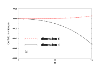
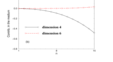
  Figure 3: Contributions from dimension 4 and dimension 6 operators to the moments both in the vacuum and in the nuclear medium in GeV^-2n.

• The mass shift is coming from the changes in the contributions from each dimension. Hence, for comparison, in Fig.4, we plot the contributions coming from each dimension in the vacuum and in the nuclear medium. One notes that effectively, each contributions becomes smaller in nuclear medium. Numerically, the ratio between the changes in dimension 4 operators and dimension 6 operators are roughly given by (dimension 4 : dimension 6 $\simeq 3:1$).

  

  

  Figure 4: Contribution to the moments in the vacuum and in the nuclear medium from (a) dimension 4 operators and (b) dimension 6 operators.

• The changes in dimension 4 operators are dominated by the changes in the scalar gluon condensate[21]. This is evident by comparing $\phi^{4}_{b}$ and $\phi^{4}_{c}$ in table 1. The comparison between $\phi^{4}_{b}$ and $\phi^{4}_{c}$ is enough to compare its contribution to the moments, because the Wilson coefficients multiplying them are the same in the large $n$ limit. Moreover, $b_{n}=c_{n}\propto n^{3}$ and $b_{n}-c_{n}\propto n$ such that $b_{n}\sim c_{n}$ at moderate $n$.

  That is not quite so for the dimension 6 operators. Here, the Wilson coefficients multiplying $\phi^{6}_{x},..$’s given in eq.(34) are also defined such that they are equal in the large $n$ limit and are proportional to $n^{5}$. However, the difference in the Wilson coefficients differ by only one power of $n$, that is, the difference between Wilson coefficients are of order $n^{4}$. Therefore, the Wilson coefficients are substantially different at the value of our interest, which is smaller than $n=10$, and become similar only at very large value of $n>100$. Hence, we will analyze each contribution from dimension 6 more in detail to identify the important contributions.

  In Fig.5 (a), we have plotted the density dependent part of the scalar, twist-2 and twist-4 contributions. As can be seen, the important contributions are the scalar operators. And among the scalar operators, the contributions coming from $\phi^{6}_{t}$ is more important than that from $\phi^{6}_{s}$. It should be noted that this is so because of the relatively large Wilson coefficients at small $n$ values. The relative importance among the scalar operators are the same also in the vacuum. The next important set of operators are the twist-4 operators. In Fig.5 (b), we plot the contributions from twist-4 operators, which has no vacuum expectation values. The most important contribution is coming from $\langle G^{a}_{\mu\nu}G^{a}_{\mu\nu;\alpha\beta}\rangle$, which contributes to $\phi^{6}_{x}$. Here, the Wilson coefficients are similar at least among the twist-4 operators and the relative importance can be read off from Table 1.

  

  

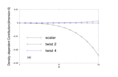
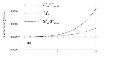
  Figure 5: (a) shows the contributions from the density dependent part of the dimension 6 scalar , twist-4 and twist-2 operators to the moments. (b) shows the individual contributions of the twist-4 operators.

  

  

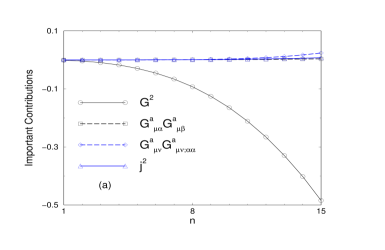
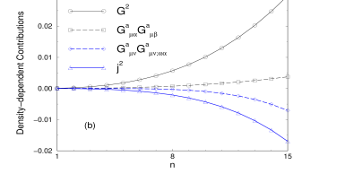
  Figure 6: (a) shows the important contributions to the moments coming from scalar operators of dimension 4 and dimension 6. (b) shows the density dependent part of (a), i.e. the density dependent changes in the condensates.

• We finally compare the dominant contributions from dimension 4 and dimension 6 operators to the moments. In Fig. 6 (a), we show the total contributions of the scalar dimension 4 and scalar dimension 6 operators to the moments. As can be seen from the figure, the dominant contributions from dimension 6 operators have opposite sign from dimension 4 operator and reduces its contribution. This reduction is enhanced for the density dependent part. This is shown in Fig. 6 (b). The reason why the change in the dimension 6 operator are greater is clear. The gluon condensate eq.(46), which is the dominant dim 4 operator, changes in nuclear matter only by 6 %, whereas, the scalar four quark condensate eq.(48), which is the dominant dim 6 operator, changes by almost 70%. Therefore, although the Wilson coefficients are smaller for dimension 6 operator, the density dependent part of dimension 6 operator are large such that it cancels the the contribution from dimension 4 operator non-trivially.

  Hence, the reason why the mass shift gets smaller compared to just taking into account dimension 4 operators is because the density dependent changes coming from dimension 4 and dimension 6 operators tend to cancel each other. Therefore, taking into account dimension 6 operators would effectively be equal to a smaller change in the dimension 4 condensate in the previous result[21], which would have given a smaller mass shift.

5 Conclusion

In this paper we have calculated the OPE of the correlation function between two vector currents made of heavy quarks up to dimension 6 operators with any tensor structure. The formidable task was to categorize and calculate the corresponding Wilson coefficients of dimension 6 twist-4 gluon operators. This is a first attempt to establish the three independent twist-4 gluon operators in terms of operator basis.

Using this result, we have applied our OPE to analyze the mass shift of $J/\psi$ in nuclear medium using QCD moment sum rules for the heavy quark system. This is a generalization of our previous result[21], where we calculated the mass shift using the OPE only up to dimension 4 operators. Unfortunately, the nucleon expectation values of the dimension 6 operators are not as reliable as the dimension 4 operators. Nevertheless, using an order of magnitude estimate for the matrix elements, we find that the mass of $J/\psi$ would decrease by about $4$ MeV in the nuclear medium. This is $3$ MeV smaller than the previous result on including only dimension 4 operators, and shows that the dimension 6 effect is about 40% correction of the dimension 4 effects and goes in the opposite direction. This result seems consistent with the notion that the higher dimensional correction in the vacuum QCD sum rule for the heavy quark system goes like $\left(G^{2}/m^{4}_{c}\right)^{K}$ in the $r_{n}=\frac{M_{n}(\xi=0)}{M_{n-1}(\xi=0)}$ with alternating signs with $K$[29]. This also seems to be true in medium and the true mass shift is expected to lie between $-4$ and $-7$ MeV.

The resulting value of mass shift, is also consistent with the more recent estimates using a totally different approach[17, 18]. This is a result for a $J/\psi$ at rest with respect to the nuclear medium. However, since we have calculated the OPE for a general external four momentum, our results can be easily and reliably generalized to study the moving $J/\psi$[24] and also to finite temperature[30], which would be also interesting in relation to the ongoing discussion of $J/\psi$ suppression in RHIC due to a comover model.

6 Acknowledgement

This work was supported by KOSEF grant number 1999-2-111-005-5, by the BK 21 project of the Korean Ministry of Education and by the Yonsei university research grant. We would like to thank T. Hatsuda, A. Hayashigaki, and W. Weise for useful discussions. We particularly thank D. Kharzeev and P. Morath for pointing out the difference in reference [16] and [17].

Appendix A Identities for spin-2 dimension 6 gluon operators

The spin-2 dimension 6 gluon operators in eq.(2) are not independent. The following relations holds among them.

$$G^{a}_{\kappa\lambda;\mu}G^{a}_{\nu\kappa;\lambda} = G^{a}_{\kappa\lambda;\mu}\cdot\frac{1}{2}(G^{a}_{\lambda\nu;\kappa}+G^{a}_{\nu\kappa;\lambda})=-\frac{1}{2}G^{a}_{\kappa\lambda;\mu}G^{a}_{\kappa\lambda;\nu}$$ (71)

$$G^{a}_{\mu\kappa;\lambda}G^{a}_{\kappa\lambda;\nu} = \frac{1}{2}\left(G^{a}_{\lambda\mu;\kappa}+G^{a}_{\mu\kappa;\lambda}\right)\cdot G^{a}_{\kappa\lambda;\nu}=-\frac{1}{2}G^{a}_{\kappa\lambda;\mu}G^{a}_{\kappa\lambda;\nu}$$ (72)

$$G^{a}_{\mu\kappa;\nu}G^{a}_{\kappa\lambda;\lambda} = -G^{a}_{\mu\kappa;\nu\lambda}G^{a}_{\kappa\lambda}=-(G^{a}_{\mu\kappa;\lambda\nu}+gf^{abc}G^{b}_{\mu\kappa}G^{c}_{\nu\lambda})G^{a}_{\kappa\lambda}$$

$$= (-)gfG^{3}_{\mu\nu}+G^{a}_{\mu\kappa;\lambda}G^{a}_{\kappa\lambda;\nu}$$

$${\rm Or,}$$

$$gfG^{3}_{\mu\nu} = G^{a}_{\mu\kappa;\lambda}G^{a}_{\kappa\lambda;\nu}-G^{a}_{\mu\kappa;\nu}G^{a}_{\kappa\lambda;\lambda}$$ (73)

$$= -\left(\frac{1}{2}G^{a}_{\kappa\lambda;\mu}G^{a}_{\kappa\lambda;\nu}+G^{a}_{\mu\kappa;\nu}G^{a}_{\kappa\lambda;\lambda}\right)$$

$$G^{a}_{\kappa\lambda;\lambda}G^{a}_{\mu\kappa;\nu} = -G^{a}_{\kappa\lambda;\lambda\nu}G^{a}_{\mu\kappa}=-\left(G^{a}_{\kappa\lambda;\nu\lambda}+gf^{abc}G^{b}_{\kappa\lambda}G^{c}_{\lambda\nu}\right)G^{a}_{\mu\kappa}$$ (74)

$$= +G^{a}_{\kappa\lambda;\nu}G^{a}_{\mu\kappa;\lambda}-g{\cal G}^{3}_{\mu\nu}=G^{a}_{\mu\kappa;\nu}G^{a}_{\kappa\lambda;\lambda}$$

$$G^{a}_{\mu\kappa;\lambda}G^{a}_{\nu\lambda;\kappa} = -G^{a}_{\mu\kappa;\lambda\kappa}G^{a}_{\nu\lambda}=-\left(G^{a}_{\mu\kappa;\kappa\lambda}+gf^{abc}G^{b}_{\mu\kappa}G^{c}_{\lambda\kappa}\right)G^{a}_{\nu\lambda}$$ (75)

$$= G^{a}_{\mu\kappa;\kappa}G^{a}_{\nu\lambda;\lambda}-g{\cal G}^{3}_{\mu\nu}$$

$$= G^{a}_{\mu\kappa;\kappa}G^{a}_{\nu\lambda;\lambda}+\frac{1}{2}G^{a}_{\kappa\lambda;\mu}G^{a}_{\kappa\lambda;\nu}+G^{a}_{\mu\kappa;\nu}G^{a}_{\kappa\lambda;\lambda}$$

$$G^{a}_{\mu\kappa;\lambda}G^{a}_{\nu\kappa;\lambda} = -G^{a}_{\mu\kappa;\lambda\lambda}G^{a}_{\nu\kappa}=-g\left(2f^{abc}G^{b}_{\mu\lambda}G^{c}_{\kappa\lambda}+j^{a}_{\mu;\kappa}-j^{a}_{\kappa;\mu}\right)G^{a}_{\nu\kappa}$$ (76)

$$= (-2)g{\cal G}^{3}_{\mu\nu}+g^{2}j^{a}_{\mu}j^{a}_{\nu}-gj^{a}_{\kappa}G^{a}_{\nu\kappa;\mu}$$

$$= G^{a}_{\kappa\lambda;\mu}G^{a}_{\kappa\lambda;\nu}+2G^{a}_{\mu\kappa;\nu}G^{a}_{\kappa\lambda;\lambda}+g^{2}j^{a}_{\mu}j^{a}_{\nu}-G^{a}_{\mu\kappa;\nu}G^{a}_{\kappa\lambda;\lambda}$$

$$= G^{a}_{\mu\kappa;\nu}G^{a}_{\kappa\lambda;\lambda}+g^{2}j^{a}_{\mu}j^{a}_{\nu}+G^{a}_{\kappa\lambda;\mu}G^{a}_{\kappa\lambda;\nu}$$

Using these, one can reduce the operators in eq.(2) to the three independent operators in eq.(5).

Appendix B Current Conservation in the Polarization Operators

Let us consider the polarization of vector currents defined in eq.(6). When the current is Hermitian, i.e. $j_{\mu}=j_{\mu}^{\dagger}$, the contribution from spin-2 dimension 4 operator can in general be written in terms of the following four independent terms.

$$\Pi_{\mu\nu}(q)=\frac{1}{Q^{2}}\left[\theta^{1}_{\mu\nu}+\frac{q^{\alpha}q^{\beta}q_{\mu}q_{\nu}}{Q^{4}}\theta^{2}_{\alpha\beta}+\frac{q^{\alpha}q_{\nu}}{Q^{2}}\theta^{3}_{\mu\alpha}+\frac{q^{\alpha}q_{\mu}}{Q^{2}}\theta^{3}_{\nu\alpha}+g_{\mu\nu}\frac{q^{\alpha}q^{\beta}}{Q^{2}}\theta^{4}_{\alpha\beta}\right]$$ (77)

Imposing current conservation, on finds,

$$\theta^{1}_{\mu\nu} = \theta^{3}_{\mu\nu}$$

$$\theta^{2}_{\mu\nu} = \theta^{1}_{\mu\nu}+\theta^{4}_{\mu\nu}$$ (78)

Similar relations holds for higher dimensional operator. This is the operator form of showing the existence of two independent polarization directions in medium for eq.(6).

Summarizing similar relations for different spins and dimensions, we have

1. dimension 4 and spin 2

   $$\Pi^{4,2}_{\mu\nu}(q)=\frac{1}{Q^{2}}\left[{\cal I}^{2}_{\mu\nu}+\frac{1}{Q^{2}}(q_{\rho}q_{\mu}{\cal I}^{2}_{\rho\nu}+q_{\rho}q_{\nu}{\cal I}^{2}_{\rho\mu})+g_{\mu\nu}\frac{q_{\rho}q_{\sigma}}{Q^{2}}{\cal J}^{2}_{\rho\sigma}+\frac{q_{\mu}q_{\nu}q_{\rho}q_{\sigma}}{Q^{4}}({\cal I}^{2}_{\rho\sigma}+{\cal J}^{2}_{\rho\sigma})\right]$$

2. dimension 6 and spin 2

   $$\Pi^{6,2}_{\mu\nu}(q)=\frac{1}{(Q^{2})^{2}}\left[I^{2}_{\mu\nu}+\frac{1}{Q^{2}}(q_{\rho}q_{\mu}I^{2}_{\rho\nu}+q_{\rho}q_{\nu}I^{2}_{\rho\mu})+g_{\mu\nu}\frac{q_{\rho}q_{\sigma}}{Q^{2}}J^{2}_{\rho\sigma}+\frac{q_{\mu}q_{\nu}q_{\rho}q_{\sigma}}{Q^{4}}(I^{2}_{\rho\sigma}+J^{2}_{\rho\sigma})\right]$$

3. dimension 6 and spin 4

   $$\Pi^{6,4}_{\mu\nu}(q) = \frac{q_{\kappa}q_{\lambda}}{(Q^{2})^{3}}\bigg{[}~{}I^{4}_{\kappa\lambda\mu\nu}+\frac{1}{Q^{2}}(q_{\rho}q_{\mu}I^{4}_{\kappa\lambda\rho\nu}+q_{\rho}q_{\nu}I^{4}_{\kappa\lambda\rho\mu})+g_{\mu\nu}\frac{q_{\rho}q_{\sigma}}{Q^{2}}J^{4}_{\kappa\lambda\rho\sigma}$$

   $$+\frac{q_{\mu}q_{\nu}q_{\rho}q_{\sigma}}{Q^{4}}(I^{4}_{\kappa\lambda\rho\sigma}+J^{4}_{\kappa\lambda\rho\sigma})\bigg{]}$$

Appendix C Propagators

Here we summarize the quark propagator in the presence of the external gauge field in the fixed point gauge[23].

$$iS(p) \equiv \int d^{4}xe^{ipx}\,iS(x,0)$$ (79)

$$= iS^{(0)}(p)+\int d^{4}xe^{ipx}\,g\int d^{4}ziS^{(0)}(x-z)i\not\!A(z)iS^{(0)}(z)$$

$$+\int d^{4}xe^{ipx}\,g^{2}\int d^{4}z^{\prime}d^{4}ziS^{(0)}(x-z^{\prime})i\not\!A(z^{\prime})iS^{(0)}(z^{\prime}-z)i\not\!A(z)iS^{(0)}(z)$$

$$+\cdots$$

and

$$i{\tilde{S}}(p) \equiv \int d^{4}xe^{-ipx}\,iS(0,x).$$ (80)

In the fixed point gauge, we write the field in terms of covariant operators,

$$A_{\mu}(x) = \frac{1}{2\cdot 0!}x_{\rho}G_{\rho\mu}(0)+\frac{1}{3\cdot 1!}x_{\alpha}x_{\rho}\left(D_{\alpha}G_{\rho\mu}(0)\right)$$ (81)

$$+\frac{1}{4\cdot 2!}x_{\alpha}x_{\beta}x_{\rho}\left(D_{\alpha}D_{\beta}G_{\rho\mu}(0)\right)+\cdots$$

Collecting terms, we can write the full propagator in terms of gauge covariant fields. A few symbols are used for convenience:

$${\hat{x}}_{\alpha}\equiv-i\frac{\stackrel{{\scriptstyle\rightarrow}}{{\partial}}}{\partial p},~{}~{}~{}\stackrel{{\scriptstyle\leftarrow}}{{x}}_{\alpha}\equiv i\frac{\stackrel{{\scriptstyle\leftarrow}}{{\partial}}}{\partial p},$$ (82)

and

$$\{\alpha,\,\beta\}=\frac{1}{\not\!p-m}\gamma_{\alpha}\frac{1}{\not\!p-m}\gamma_{\beta}\frac{1}{\not\!p-m}$$

$$\{\alpha,\,\beta,\,\sigma\}=\frac{1}{\not\!p-m}\gamma_{\alpha}\frac{1}{\not\!p-m}\gamma_{\beta}\frac{1}{\not\!p-m}\gamma_{\sigma}\frac{1}{\not\!p-m}$$

$$~{}~{}~{}\vdots,$$ (83)

and $P(\alpha,\beta,\gamma...)$ means sum of all possible permutations in $\alpha,\beta,\gamma...$.

Here we simply list the propagators.

1. $iS^{(0)}(p)=i{\tilde{S}}^{(0)}(p)$

   $$=\frac{i}{\not\!p-m}$$

2. $iS_{G}(p)=i{\tilde{S}}_{G}(p)$

   $$= iS^{(0)}(p)~{}i(\gamma_{\beta}\cdot\frac{1}{2}{\hat{x}}_{\alpha}G_{\alpha\beta})~{}iS^{(0)}(p)=\frac{1}{2}\,G_{\alpha\beta}\{\beta,\,\alpha\}$$

   $$= iS^{(0)}(p)~{}i(\gamma_{\beta}\cdot\frac{1}{2}\stackrel{{\scriptstyle\leftarrow}}{{x}}_{\alpha}G_{\alpha\beta})~{}iS^{(0)}(p)=-\frac{1}{2}\,G_{\alpha\beta}\{\alpha,\,\beta\}$$

3. $iS_{G^{2}}(p)=i{\tilde{S}}_{G^{2}}(p)$

   $$= iS^{(0)}(p)~{}i(\gamma_{\beta}\cdot\frac{1}{2}{\hat{x}}_{\alpha}G_{\alpha\beta})~{}iS^{(0)}(p)~{}i(\gamma_{\sigma}\cdot\frac{1}{2}{\hat{x}}_{\rho}G_{\rho\sigma})~{}iS^{(0)}(p)$$

   $$= -\frac{i}{4}G_{\alpha\beta}G_{\rho\sigma}\Big{[}\{\beta,\alpha,\sigma,\rho\}+\{\beta,\sigma,P(\alpha,\rho)\}\Big{]}$$

   $$= iS^{(0)}(p)~{}i(\gamma_{\beta}\cdot\frac{1}{2}\stackrel{{\scriptstyle\leftarrow}}{{x}}_{\alpha}G_{\alpha\beta})~{}iS^{(0)}(p)~{}i(\gamma_{\sigma}\cdot\frac{1}{2}\stackrel{{\scriptstyle\leftarrow}}{{x}}_{\rho}G_{\rho\sigma})~{}iS^{(0)}(p)$$

   $$= -\frac{i}{4}G_{\alpha\beta}G_{\rho\sigma}\Big{[}\{\alpha,\beta,\rho,\sigma\}+\{P(\alpha,\rho),\beta,\sigma\}\Big{]}$$

4. As for $G^{3}$ part,

   • $iS_{G^{3}}(p)$

     $$= iS^{(0)}(p)~{}i(\gamma_{\beta}\frac{1}{2}{\hat{x}}_{\alpha}G_{\alpha\beta})~{}iS^{(0)}(p)~{}i(\gamma_{\sigma}\frac{1}{2}{\hat{x}}_{\rho}G_{\rho\sigma})~{}iS^{(0)}(p)~{}i(\gamma_{\lambda}\frac{1}{2}{\hat{x}}_{\kappa}G_{\kappa\lambda})~{}iS^{(0)}(p)$$

     $$= -\frac{1}{8}G_{\alpha\beta}G_{\rho\sigma}G_{\kappa\lambda}\Big{[}\{\beta,\alpha,\sigma,\rho,\lambda,\kappa\}+\{\beta,\alpha,\sigma,\lambda,P(\rho,\kappa)\}$$

     $$~{}~{}~{}~{}~{}~{}~{}+\{\beta,\sigma,P(\alpha,\rho),\lambda,\kappa\}+\{\beta,\sigma,\rho,\lambda,P(\alpha,\kappa)\}$$

     $$~{}~{}~{}~{}~{}~{}~{}+\{\beta,\sigma,\alpha,\lambda,P(\rho,\kappa)\}+\{\beta,\sigma,\lambda,P(\alpha,\rho,\kappa)\}\Big{]}$$

   • $i{\tilde{S}}_{G^{3}}(p)$

     $$= iS^{(0)}(p)~{}i(\gamma_{\beta}\frac{1}{2}{\stackrel{{\scriptstyle\leftarrow}}{{x}}}_{\alpha}G_{\alpha\beta})~{}iS^{(0)}(p)~{}i(\gamma_{\sigma}\frac{1}{2}{\stackrel{{\scriptstyle\leftarrow}}{{x}}}_{\rho}G_{\rho\sigma})~{}iS^{(0)}(p)~{}i(\gamma_{\lambda}\frac{1}{2}{\stackrel{{\scriptstyle\leftarrow}}{{x}}}_{\kappa}G_{\kappa\lambda})~{}iS^{(0)}(p)$$

     $$= \frac{1}{8}G_{\alpha\beta}G_{\rho\sigma}G_{\kappa\lambda}\Big{[}\{\alpha,\beta,\rho,\sigma,\kappa,\lambda\}+\{P(\alpha,\rho),\beta,\sigma,\kappa,\lambda\}$$

     $$~{}~{}~{}~{}~{}~{}~{}+\{\alpha,\beta,P(\kappa,\rho),\sigma,\lambda\}+\{P(\alpha,\kappa,\rho),\beta,\sigma,\lambda\}$$

     $$~{}~{}~{}~{}~{}~{}~{}+\{P(\alpha,\rho),\beta,\kappa,\sigma,\lambda\}+\{P(\alpha,\kappa),\beta,\rho,\sigma,\lambda\}\Big{]}$$

5. As for $DG$ part,

   • $iS_{DG}(p)$

     $$= iS^{(0)}(p)~{}i(\gamma_{\sigma}\cdot\frac{1}{3}{\hat{x}}_{\alpha}{\hat{x}}_{\beta}D_{\alpha}G_{\beta\sigma})~{}iS^{(0)}(p)$$

     $$= \frac{i}{3}D_{\alpha}G_{\beta\sigma}\{\sigma,P(\alpha,\beta)\}$$

   • $i{\tilde{S}}_{DG}(p)$

     $$= iS^{(0)}(p)~{}i(\gamma_{\sigma}\cdot\frac{1}{3}{\stackrel{{\scriptstyle\leftarrow}}{{x}}}_{\alpha}{\stackrel{{\scriptstyle\leftarrow}}{{x}}}_{\beta}D_{\alpha}G_{\beta\sigma})~{}iS^{(0)}(p)$$

     $$= \frac{i}{3}D_{\alpha}G_{\beta\sigma}\{P(\alpha,\beta),\sigma\}$$

6. As for $D^{2}G$ part,

   • $iS_{D^{2}G}(p)$

     $$= iS^{(0)}(p)~{}i(\gamma_{\sigma}\cdot\frac{1}{8}{\hat{x}}_{\alpha}{\hat{x}}_{\beta}{\hat{x}}_{\nu}D_{\alpha}D_{\beta}G_{\nu\sigma})~{}iS^{(0)}(p)$$

     $$= -\frac{1}{8}D_{\alpha}D_{\beta}G_{\nu\sigma}\{\sigma,P(\alpha,\beta,\nu)\}$$

   • $i{\tilde{S}}_{D^{2}G}(p)$

     $$= iS^{(0)}(p)~{}i(\gamma_{\sigma}\cdot\frac{1}{8}{\stackrel{{\scriptstyle\leftarrow}}{{x}}}_{\alpha}{\stackrel{{\scriptstyle\leftarrow}}{{x}}}_{\beta}{\stackrel{{\scriptstyle\leftarrow}}{{x}}}_{\nu}D_{\alpha}D_{\beta}G_{\nu\sigma})~{}iS^{(0)}(p)$$

     $$= +\frac{1}{8}D_{\alpha}D_{\beta}G_{\nu\sigma}\{P(\alpha,\beta,\nu),\sigma\}$$

7. As for $(DG)^{2}$ part,

   • $iS_{(DG)^{2}}(p)$

     $$= iS^{(0)}(p)~{}i(\gamma_{\kappa}\cdot\frac{1}{3}{\hat{x}}_{\alpha}{\hat{x}}_{\beta}D_{\alpha}G_{\beta\kappa})~{}iS^{(0)}(p)~{}i(\gamma_{\lambda}\cdot\frac{1}{3}{\hat{x}}_{\rho}{\hat{x}}_{\sigma}D_{\rho}G_{\sigma\lambda})~{}iS^{(0)}(p)$$

     $$= \frac{i}{9}D_{\alpha}G_{\beta\kappa}D_{\rho}G_{\sigma\lambda}\Big{[}\{\kappa,P(\alpha,\beta),\lambda,P(\rho,\sigma)\}$$

     $$~{}~{}~{}+\{\kappa,\alpha,\lambda,P(\beta,\rho,\sigma)\}+\{\kappa,\beta,\lambda,P(\alpha,\rho,\sigma)\}+\{\kappa,\lambda,P(\alpha,\beta,\rho,\sigma)\}\Big{]}$$

   • $i{\tilde{S}}_{(DG)^{2}}(p)$

     $$= iS^{(0)}(p)~{}i(\gamma_{\kappa}\cdot\frac{1}{3}{\stackrel{{\scriptstyle\leftarrow}}{{x}}}_{\alpha}{\stackrel{{\scriptstyle\leftarrow}}{{x}}}_{\beta}D_{\alpha}G_{\beta\kappa})~{}iS^{(0)}(p)~{}i(\gamma_{\lambda}\cdot\frac{1}{3}{\stackrel{{\scriptstyle\leftarrow}}{{x}}}_{\rho}{\stackrel{{\scriptstyle\leftarrow}}{{x}}}_{\sigma}D_{\rho}G_{\sigma\lambda})~{}iS^{(0)}(p)$$

     $$= \frac{i}{9}D_{\alpha}G_{\beta\kappa}D_{\rho}G_{\sigma\lambda}\Big{[}\{P(\alpha,\beta),\kappa,P(\rho,\sigma),\lambda\}$$

     $$~{}~{}~{}+\{P(\alpha,\beta,\rho),\kappa,\sigma,\lambda\}+\{P(\alpha,\beta,\sigma),\kappa,\rho,\lambda\}+\{P(\alpha,\beta,\rho,\sigma),\kappa,\lambda\}\Big{]}$$

8. As for $GD^{2}G$ part,

   • $iS_{GD^{2}G}(p)$

     $$= iS^{(0)}(p)~{}i(\gamma_{\beta}\cdot\frac{1}{2}{\hat{x}}_{\alpha}G_{\alpha\beta})~{}iS^{(0)}(p)~{}i(\gamma_{\sigma}\cdot\frac{1}{8}{\hat{x}}_{\rho}{\hat{x}}_{\kappa}{\hat{x}}_{\lambda}D_{\rho}D_{\kappa}G_{\lambda\sigma})~{}iS^{(0)}$$

     $$= \frac{i}{16}G_{\alpha\beta}D_{\rho}D_{\kappa}G_{\lambda\sigma}\Big{[}\{\beta,\alpha,\sigma,P(\rho,\kappa,\lambda)\}+\{\beta,\sigma,P(\alpha,\rho,\kappa,\lambda)\}\Big{]}$$

   • $i{\tilde{S}}_{GD^{2}G}(p)$

     $$= iS^{(0)}(p)~{}i(\gamma_{\beta}\cdot\frac{1}{2}{\stackrel{{\scriptstyle\leftarrow}}{{x}}}_{\alpha}G_{\alpha\beta})~{}iS^{(0)}(p)~{}i(\gamma_{\sigma}\cdot\frac{1}{8}{\stackrel{{\scriptstyle\leftarrow}}{{x}}}_{\rho}{\stackrel{{\scriptstyle\leftarrow}}{{x}}}_{\kappa}{\stackrel{{\scriptstyle\leftarrow}}{{x}}}_{\lambda}D_{\rho}D_{\kappa}G_{\lambda\sigma})~{}iS^{(0)}$$

     $$= \frac{i}{16}G_{\alpha\beta}D_{\rho}D_{\kappa}G_{\lambda\sigma}\Big{[}\{\alpha,\beta,P(\rho,\kappa,\lambda),\sigma\}+\{P(\alpha,\rho),\beta,P(\kappa,\lambda),\sigma\}$$

     $$~{}~{}~{}~{}~{}~{}~{}+\{P(\alpha,\kappa),\beta,P(\rho,\lambda),\sigma\}+\{P(\alpha,\lambda),\beta,P(\kappa,\rho),\sigma\}$$

     $$~{}~{}~{}~{}~{}~{}~{}+\{P(\alpha,\kappa,\lambda),\beta,\rho,\sigma\}+\{P(\alpha,\rho,\lambda),\beta,\kappa,\sigma\}$$

     $$~{}~{}~{}~{}~{}~{}~{}+\{P(\alpha,\kappa,\rho),\beta,\lambda,\sigma\}+\{P(\alpha,\rho,\kappa,\lambda),\beta,\sigma\}\Big{]}$$

9. As for $D^{2}GG$ part,

   • $iS_{D^{2}GG}(p)$

     $$= iS^{(0)}(p)~{}i(\gamma_{\sigma}\cdot\frac{1}{8}{\hat{x}}_{\rho}{\hat{x}}_{\kappa}{\hat{x}}_{\lambda}D_{\rho}D_{\kappa}G_{\lambda\sigma})~{}iS^{(0)}(p)~{}i(\gamma_{\beta}\cdot\frac{1}{2}{\hat{x}}_{\alpha}G_{\alpha\beta})~{}iS^{(0)}(p)$$

     $$= \frac{i}{16}D_{\rho}D_{\kappa}G_{\lambda\sigma}G_{\alpha\beta}\Big{[}\{\sigma,P(\rho,\kappa,\lambda),\beta,\alpha\}+\{\sigma,P(\kappa,\lambda),\beta,P(\alpha,\rho)\}$$

     $$~{}~{}~{}~{}~{}~{}~{}+\{\sigma,\rho,\beta,P(\kappa,\lambda,\alpha)\}+\{\sigma,\beta,P(\rho,\kappa,\lambda,\alpha)\}$$

     $$~{}~{}~{}~{}~{}~{}~{}+\{\sigma,P(\kappa,\rho),\beta,P(\alpha,\lambda)\}+\{\sigma,\kappa,\beta,P(\alpha,\lambda,\rho)\}$$

     $$~{}~{}~{}~{}~{}~{}~{}+\{\sigma,P(\lambda,\rho),\beta,P(\alpha,\kappa)\}+\{\sigma,\lambda,\beta,P(\rho,\alpha,\kappa)\}\Big{]}$$

   • $i{\tilde{S}}_{D^{2}GG}(p)$

     $$= iS^{(0)}(p)~{}i(\gamma_{\sigma}\cdot\frac{1}{8}{\stackrel{{\scriptstyle\leftarrow}}{{x}}}_{\rho}{\stackrel{{\scriptstyle\leftarrow}}{{x}}}_{\kappa}{\stackrel{{\scriptstyle\leftarrow}}{{x}}}_{\lambda}D_{\rho}D_{\kappa}G_{\lambda\sigma})~{}iS^{(0)}(p)~{}i(\gamma_{\beta}\cdot\frac{1}{2}{\stackrel{{\scriptstyle\leftarrow}}{{x}}}_{\alpha}G_{\alpha\beta})~{}iS^{(0)}(p)$$

     $$= \frac{i}{16}D_{\rho}D_{\kappa}G_{\lambda\sigma}G_{\alpha\beta}\Big{[}\{P(\rho,\kappa,\lambda),\sigma,\alpha,\beta\}+\{P(\rho,\kappa,\lambda,\alpha),\sigma,\beta\}\Big{]}$$

Appendix D spin structure of operators of dimension 6

In computing the Wilson coefficients we used the following reduction of the Lorentz indices to the spin-2 operators.

$$f^{abc}G^{a}_{\mu\nu}G^{b}_{\alpha\beta}G^{c}_{\rho\sigma} = A_{\mu\alpha}c_{\nu\rho\beta\sigma}-A_{\mu\beta}c_{\nu\rho\alpha\sigma}-A_{\nu\alpha}c_{\mu\rho\beta\sigma}+A_{\nu\beta}c_{\mu\rho\alpha\sigma}$$ (84)

$$-A_{\mu\rho}c_{\nu\alpha\sigma\beta}+A_{\mu\sigma}c_{\nu\alpha\rho\beta}+A_{\nu\rho}c_{\mu\alpha\sigma\beta}-A_{\nu\sigma}c_{\mu\alpha\rho\beta}$$

$$+A_{\alpha\rho}c_{\beta\mu\sigma\nu}-A_{\alpha\sigma}c_{\beta\mu\rho\nu}-A_{\beta\rho}c_{\alpha\mu\sigma\nu}+A_{\beta\sigma}c_{\alpha\mu\rho\nu}$$

$$G^{a}_{\mu_{1}\nu_{1}}G^{a}_{\mu_{2}\nu_{2};\alpha\beta} = K_{\alpha\beta}c_{\mu_{1}\mu_{2}\nu_{1}\nu_{2}}$$ (85)

$$+P_{\beta\mu_{1}}c_{\alpha\mu_{2}\nu_{1}\nu_{2}}-P_{\beta\nu_{1}}c_{\alpha\mu_{2}\mu_{1}\nu_{2}}$$

$$~{}+J_{\alpha\mu_{2}}c_{\beta\mu_{1}\nu_{2}\nu_{1}}-J_{\alpha\nu_{2}}c_{\beta\mu_{1}\mu_{2}\nu_{1}}$$

$$+Q_{\beta\mu_{2}}c_{\alpha\mu_{1}\nu_{2}\nu_{1}}-Q_{\beta\nu_{2}}c_{\alpha\mu_{1}\mu_{2}\nu_{1}}$$

$$~{}+W_{\alpha\mu_{1}}c_{\beta\mu_{2}\nu_{1}\nu_{2}}-W_{\alpha\nu_{1}}c_{\beta\mu_{2}\mu_{1}\nu_{2}}$$

$$+L_{\mu_{1}\mu_{2}}d_{\beta\nu_{1}\alpha\nu_{2}}-L_{\nu_{1}\mu_{2}}d_{\beta\mu_{1}\alpha\nu_{2}}$$

$$~{}-L_{\mu_{1}\nu_{2}}d_{\beta\nu_{1}\alpha\mu_{2}}+L_{\nu_{1}\nu_{2}}d_{\beta\mu_{1}\alpha\mu_{2}}$$

$$+M_{\mu_{1}\mu_{2}}d_{\beta\alpha\nu_{1}\nu_{2}}-M_{\nu_{1}\mu_{2}}d_{\alpha\beta\mu_{1}\nu_{2}}$$

$$~{}-M_{\mu_{1}\nu_{2}}d_{\alpha\beta\nu_{1}\mu_{2}}+M_{\nu_{1}\nu_{2}}d_{\alpha\beta\mu_{1}\mu_{2}}$$

$$+T_{\mu_{1}\mu_{2}}d_{\beta\nu_{2}\alpha\nu_{1}}-T_{\nu_{1}\mu_{2}}d_{\beta\nu_{2}\alpha\mu_{1}}$$

$$~{}-T_{\mu_{1}\nu_{2}}d_{\beta\mu_{2}\alpha\nu_{1}}+T_{\nu_{1}\nu_{2}}d_{\beta\mu_{2}\alpha\mu_{1}},$$

where

$$c_{\alpha\beta\mu\nu} \equiv g_{\alpha\beta}g_{\mu\nu}-g_{\alpha\nu}g_{\mu\beta},$$

$$d_{\alpha\beta\mu\nu} \equiv g_{\alpha\beta}g_{\mu\nu}$$ (86)

and, if we take 3 operators, $ddgg1\equiv G^{a}_{\kappa\lambda}G^{a}_{\kappa\lambda;\mu\nu},~{}ddgg2\equiv-g^{2}j^{a}_{\mu}j^{a}_{\nu},$ and $ddgg3\equiv G^{a}_{\mu\kappa}G^{a}_{\kappa\lambda;\lambda\nu}$ as our basis, we get

$$A=(ddgg1+2ddgg3)/4,$$

$$K=2P=2J=(13ddgg1+ddgg2+19ddgg3)/80,$$

$$Q=W=(-27ddgg1+ddgg2-61ddgg3)/160,$$

$$L=(4ddgg1+3ddgg2+7ddgg3)/40,$$

$$M=(29ddgg1+13ddgg2+47ddgg3)/160,$$

$$T=(-6ddgg1+3ddgg2-13ddgg3)/40.$$ (87)

As for the spin 4 part, we have a simpler reduction:

$$G^{a}_{\mu_{1}\nu_{1}}G^{a}_{\mu_{2}\nu_{2};\alpha\beta} = W_{\alpha\beta\mu_{1}\mu_{2}}g_{\nu_{1}\nu_{2}}+W_{\alpha\beta\nu_{1}\nu_{2}}g_{\mu_{1}\mu_{2}}$$ (88)

$$-W_{\alpha\beta\mu_{1}\nu_{2}}g_{\nu_{1}\mu_{2}}-W_{\alpha\beta\nu_{1}\mu_{2}}g_{\mu_{1}\nu_{2}},$$

where

$$W_{\alpha\beta\mu_{1}\mu_{2}}=\frac{1}{2}G^{a}_{\mu_{1}\kappa}G^{a}_{\mu_{2}\kappa;\alpha\beta}.$$ (89)

Appendix E Integrations with respect to Feynman Parameter

In general, after Feynman integration, one can write the polarizations in terms of linear sums of $J$’s defined in eq.(13).

$$\Pi(q)=Q^{-a}\left[\,a_{0}J_{0}+a_{1}J_{1}+a_{2}J_{2}+\cdots\,\,+a_{k}J_{k}\right].$$ (90)

To reduce the polarization function into this final form, we use the following steps and identities.

After the Feynman integral, the polarization function will be a sum of $I{mn}$’s:

$$I^{mn}_{N}(Q^{2},m^{2})\equiv\int^{1}_{0}dx\frac{x^{n}(1-x)^{m}}{\left[m^{2}+Q^{2}x(1-x)\right]^{N}}=I^{nm}_{N}(Q^{2},m^{2})$$ (91)

We then follow the following steps.

1. $I^{mn}$ can be expressed in terms of $I^{n}_{N}\equiv I^{nn}_{N}$ using the following identity.

   $$x^{n}+(1-x)^{n} = 1-\Big{\{}~{}_{n}C_{1}x^{n-1}(1-x)+_{n}C_{2}x^{n-2}(1-x)^{2}+\cdots+_{n}C_{k}x^{n-k}(1-x)^{k}$$

   $$+\cdots+_{n}C_{n-1}x(1-x)^{n-1}\Big{\}}$$

   $$= 1-_{n}\!C_{1}\{x^{n-1}(1-x)+x(1-x)^{n-1}\}$$

   $$-_{n}\!C_{2}\{x^{n-2}(1-x)^{2}+x^{2}(1-x)^{n-2}\}-\cdots$$

   $$= 1-_{n}\!C_{1}~{}x(1-x)\Big{\{}x^{n-2}+(1-x)^{n-2}\Big{\}}$$

   $$-_{n}\!C_{2}~{}x^{2}(1-x)^{2}\Big{\{}x^{n-4}+(1-x)^{n-4}\Big{\}}-\cdots$$

2. Then we can reduce $I^{n}_{N}$ to $I^{0}_{N}\equiv I_{N}$ using $I^{n}_{N}=\frac{1}{Q^{2}}(I^{n-1}_{N-1}-m^{2}I^{n-1}_{N})=\frac{1}{Q^{2}}I^{n-1}_{N-1}-\frac{1}{y}I^{n-1}_{N-1}$

3. We then introduce the dimensionless function $J_{N}(y)=\left(\frac{Q^{2}}{y}\right)^{N}I_{N}$, where $y=Q^{2}/m^{2}$.

4. Finally, we use the recurrence relation.

   $$y\,J_{N}(y)=\frac{2}{N-1}+\frac{4N-6}{N-1}J_{N-1}(y)-4J_{N}(y)$$ (92)

5. We can also integrate explicitly,

   $$J_{N}(y)=\frac{(2N-3)!!}{(N-1)!}\left[\left(\frac{s-1}{2s}\right)^{N}\sqrt{s}\log\frac{\sqrt{s}+1}{\sqrt{s}-1}+\sum^{N-1}_{k=1}\frac{(k-1)!}{(2k-1)!!}\left(\frac{s-1}{2s}\right)^{N-k}\right],$$ (93)

   where $s=1+4/y$.

Appendix F An example: evaluation of a diagram

Diagram 1a: We show the evaluation of the Feynman diagrams here. The first diagram in Fig. 1 is taken as an example.

$$i\int\frac{d^{4}k}{(2\pi)^{4}}{\rm Tr}\left[\gamma_{\mu}S^{(0)}(k+q)\gamma_{\nu}{\tilde{S}}_{G^{3}}(k)\right]$$ (94)

$$= i\int\frac{d^{4}k}{(2\pi)^{4}}{\rm Tr}\bigg{[}\gamma_{\mu}\frac{1}{\not\!k+\not\!q-m}\gamma_{\nu}\,\left(\frac{-i}{8}\right)G^{a}_{\alpha\beta}G^{b}_{\rho\sigma}G^{c}_{\kappa\lambda}t^{a}t^{b}t^{c}\Big{[}\{\alpha,\beta,\rho,\sigma,\kappa,\lambda\}+\{P(\alpha,\rho),\beta,\sigma,\kappa,\lambda\}$$

$$~{}~{}~{}+\{\alpha,\beta,P(\kappa,\rho),\sigma,\lambda\}+\{P(\alpha,\kappa,\rho),\beta,\sigma,\lambda\}+\{P(\alpha,\rho),\beta,\kappa,\sigma,\lambda\}+\{P(\alpha,\kappa),\beta,\rho,\sigma,\lambda\}\Big{]}\bigg{]}$$

$$= \frac{1}{8}\frac{i}{4}\left(f^{abc}\,G^{a}_{\alpha\beta}G^{b}_{\rho\sigma}G^{c}_{\kappa\lambda}\right)\int\frac{d^{4}k}{(2\pi)^{4}}\frac{1}{(k+q)^{2}-m^{2}}{\rm Tr}\bigg{[}\gamma_{\mu}(\not\!k+\not\!q+m)\gamma_{\nu}$$

$$~{}~{}~{}\times\Big{[}\{\alpha,\beta,\rho,\sigma,\kappa,\lambda\}+\{P(\alpha,\rho),\beta,\sigma,\kappa,\lambda\}+\{\alpha,\beta,P(\kappa,\rho),\sigma,\lambda\}$$

$$~{}~{}~{}+\{P(\alpha,\kappa,\rho),\beta,\sigma,\lambda\}+\{P(\alpha,\rho),\beta,\kappa,\sigma,\lambda\}+\{P(\alpha,\kappa),\beta,\rho,\sigma,\lambda\}\Big{]}\bigg{]}$$

$$= \frac{1}{8}\frac{i}{4}\Big{(}\,A_{\mu\alpha}c_{\nu\rho\beta\sigma}-A_{\mu\beta}c_{\nu\rho\alpha\sigma}-A_{\nu\alpha}c_{\mu\rho\beta\sigma}+A_{\nu\beta}c_{\mu\rho\alpha\sigma}-A_{\mu\rho}c_{\nu\alpha\sigma\beta}+A_{\mu\sigma}c_{\nu\alpha\rho\beta}$$

$$~{}~{}~{}~{}+A_{\nu\rho}c_{\mu\alpha\sigma\beta}-A_{\nu\sigma}c_{\mu\alpha\rho\beta}+A_{\alpha\rho}c_{\beta\mu\sigma\nu}-A_{\alpha\sigma}c_{\beta\mu\rho\nu}-A_{\beta\rho}c_{\alpha\mu\sigma\nu}+A_{\beta\sigma}c_{\alpha\mu\rho\nu}\Big{)}$$

$$\times\int\frac{d^{4}k}{(2\pi)^{4}}\frac{1}{(k+q)^{2}-m^{2}}\frac{1}{(k^{2}-m^{2})^{7}}{\rm Tr}\bigg{[}\gamma_{\mu}(\not\!k+\not\!q+m)\gamma_{\nu}$$

$$\times\Big{\{}(\not\!k+m)\gamma_{\alpha}(\not\!k+m)\gamma_{\beta}(\not\!k+m)\gamma_{\rho}(\not\!k+m)\gamma_{\sigma}(\not\!k+m)\gamma_{\kappa}(\not\!k+m)\gamma_{\lambda}(\not\!k+m)+\cdots\Big{\}}\bigg{]}$$

$$\equiv i\int\frac{d^{4}k}{(2\pi)^{4}}\frac{1}{(k+q)^{2}-m^{2}}\frac{1}{(k^{2}-m^{2})^{7}}f_{1a}(k)$$

$$= i\int\frac{d^{4}k}{(2\pi)^{4}}\left[\int^{1}_{0}dx\frac{x^{6}}{[\{k+(1-x)q\}^{2}-s^{2}]^{8}}\frac{\Gamma(8)}{\Gamma(7)}\right]f_{1a}(k)$$

$$= \frac{i}{8}\int^{1}_{0}dx\int\frac{d^{4}l}{(2\pi)^{4}}\frac{1}{[l^{2}-s^{2}]^{8}}\frac{\Gamma(8)}{\Gamma(7)}\Bigg{[}\Big{\{}-\frac{28}{3}l^{8}+\left(\frac{116}{3}m^{2}-\frac{220}{3}q^{2}t^{2}\right)l^{6}$$

$$+\left(-\frac{148}{3}m^{4}+\frac{416}{3}m^{2}q^{2}t^{2}-\frac{268}{3}q^{4}t^{4}\right)l^{4}+\left(20m^{6}-60m^{4}q^{2}t^{2}+60m^{2}q^{4}t^{4}-20q^{6}t^{6}\right)l^{2}\Big{\}}A_{\mu\nu}$$

$$+\Big{\{}(-640t^{3}+896t^{4})l^{4}+(640m^{2}t^{3}-768m^{2}t^{4})l^{2}$$

$$-128m^{4}(t^{3}-t^{4})+256m^{2}q^{2}(t^{5}-t^{6})-128q^{4}(t^{7}-t^{8})\Big{\}}q_{\mu}q_{\nu}q_{\alpha}q_{\beta}A_{\alpha\beta}$$

$$+\Big{\{}-\frac{140}{3}tl^{6}+\left(\frac{464}{3}m^{2}t+\frac{400}{3}m^{2}t^{2}+\frac{80}{3}q^{2}t^{3}\right)l^{4}$$

$$+(-148m^{4}t-112m^{4}t^{2}+96m^{2}q^{2}t^{3}+296m^{2}q^{2}t^{4}+116q^{4}t^{5}-184q^{4}t^{6})l^{2}$$

$$+(40t+24t^{2})m^{6}-(56q^{2}t^{3}-72q^{2}t^{4})m^{4}+(-8q^{4}t^{5}+72q^{4}t^{6})m^{2}+24q^{6}(t^{7}-t^{8})\Big{\}}g_{\mu\nu}q_{\alpha}q_{\beta}A_{\alpha\beta}$$

$$+\Big{\{}\left(\frac{140}{3}t-40t^{2}\right)l^{6}+(-\frac{464}{3}m^{2}t+\frac{560}{3}m^{2}t^{2})l^{4}$$

$$+(148m^{4}t-176m^{4}t^{2}-416m^{2}q^{2}t^{3}+472m^{2}q^{2}t^{4}+268q^{4}t^{5}-296q^{4}t^{6})l^{2}$$

$$-40m^{6}(t-t^{2})+120m^{4}q^{2}(t^{3}-t^{4})-120m^{2}q^{4}(t^{5}-t^{6})+40q^{6}(t^{7}-t^{8})\Big{\}}(q_{\mu}q_{\alpha}A_{\alpha\nu}+q_{\nu}q_{\alpha}A_{\alpha\mu})\Bigg{]}$$

$$= A_{\mu\nu}\frac{\pi^{2}}{Q^{4}}\left(\frac{7}{3}-y+(\frac{1}{3}+\frac{1}{6}y)J_{1}-\frac{8}{3}J_{2}\right)$$

$$+g_{\mu\nu}q_{\alpha}q_{\beta}A_{\alpha\beta}\frac{\pi^{2}}{Q^{6}}\left(\frac{5}{3}+y-(2+y)J_{1}-9J_{2}+\frac{52}{3}J_{3}-8J_{4}\right)$$

$$+q_{\mu}q_{\nu}q_{\alpha}q_{\beta}A_{\alpha\beta}\frac{\pi^{2}}{Q^{8}}\left(\frac{68}{3}-(8+4y)J_{1}-36J_{2}+\frac{88}{3}J_{3}-8J_{4}\right)$$

$$+(q_{\mu}q_{\alpha}A_{\alpha\nu}+q_{\nu}q_{\alpha})A_{\alpha\mu}\frac{\pi^{2}}{Q^{6}}\left(\frac{23}{3}-y-(\frac{2}{3}+\frac{1}{3}y)J_{1}-\frac{41}{3}J_{2}+\frac{20}{3}J_{3}\right)$$

Appendix G Moments in terms of Hypergeometric Functions ${}_{2}F_{1}$

In order to obtain moments written in terms of hypergeometric functions ${}_{2}F_{1}$ from polarizations eq.(90), we expand the polarizations in terms of $Q^{2}/m^{2}$. Here we divide $a_{0}$ and $a_{1}$ into $a_{0}=d_{1}+d_{2}y$ and $a_{1}=c_{1}+c_{2}y$. The other higher coefficients, $a_{2},a_{3},\cdots,a_{k}$ don’t contain $y$, where $y=Q^{2}/m^{2}$.

$$\Pi(q) = Q^{-a}\bigg{[}\,a_{0}+(c_{1}+c_{2}y)\int^{1}_{0}\frac{dx}{[1+x(1-x)Q^{2}/m^{2}]}+a_{2}\int^{1}_{0}\frac{dx}{[1+x(1-x)Q^{2}/m^{2}]^{2}}+$$ (95)

$$~{}~{}~{}\vdots$$

$$+a_{k}\int^{1}_{0}\frac{dx}{[1+x(1-x)Q^{2}/m^{2}]^{k}}\bigg{]}$$

$$= Q^{-a}\bigg{[}\,a_{0}+(c_{1}+c_{2}y)\int^{1}_{0}dx\sum^{\infty}_{j=0}\left\{-x(1-x)\right\}^{j}\frac{Q^{2j}}{m^{2j}}$$

$$+a_{2}\int^{1}_{0}dx\sum^{\infty}_{j=0}\left\{-x(1-x)\right\}^{j}\frac{(1+j)!}{j!}\frac{Q^{2j}}{m^{2j}}+$$

$$~{}~{}~{}\vdots$$

$$+a_{k}\int^{1}_{0}dx\sum^{\infty}_{j=0}\left\{-x(1-x)\right\}^{j}\frac{(k-1+j)!}{(k-1)!j!}\frac{Q^{2j}}{m^{2j}}\bigg{]}$$

$$= Q^{-a}\sum^{\infty}_{j=1}\Bigg{[}\,c_{1}\int^{1}_{0}dx(-1)^{j}x^{j}(1-x)^{j}\frac{Q^{2j}}{m^{2j}}+a_{2}\int^{1}_{0}dx(-1)^{j}x^{j}(1-x)^{j}(1+j)\frac{Q^{2j}}{m^{2j}}+$$

$$~{}~{}~{}\vdots$$

$$+a_{k}\int^{1}_{0}dx(-1)^{j}x^{j}(1-x)^{j}\frac{(k-1+j)!}{(k-1)!j!}\frac{Q^{2j}}{m^{2j}}-c_{2}\int^{1}_{0}dx(-1)^{j}x^{j-1}(1-x)^{j-1}\frac{Q^{2j}}{m^{2j}}\Bigg{]}$$

$$= \sum^{\infty}_{j=a/2}(-)^{a/2-1}\int^{1}_{0}dx\left\{x(1-x)\right\}^{j-1}\frac{(-Q^{2})^{j-a/2}}{m^{2j}}\bigg{[}-x(1-x)\Big{\{}c_{1}+a_{2}(1+j)$$

$$+\frac{a_{3}}{2!}(1+j)(2+j)+\cdots\,\,+\frac{a_{k}}{(k-1)!}\prod^{k-1}_{l=1}(l+j)\Big{\}}+c_{2}\bigg{]}$$

Now the $n$’s moment $M_{n}$ can be obtained from above by differentiation.

$$M_{n}(Q_{0}) = \frac{1}{n!}\left(-\frac{d}{dQ^{2}}\right)^{n}\Pi(Q^{2})$$ (104)

$$= (-)^{a/2}\frac{1}{(4m^{2})^{a/2+n}}\frac{1}{(1+\xi)^{n+1}}\bigg{[}\,c_{1}d_{1}+c_{2}d_{2}$$

$$+\frac{1}{2}\Bigg{\{}a_{2}\frac{\Gamma\left(\frac{1}{2}\right)\Gamma\left(n+\frac{a}{2}+2\right)}{\Gamma\left(n+\frac{a+3}{2}\right)}\,_{2}F_{1}(n+1,-\frac{1}{2},n+\frac{a+3}{2};\frac{\xi}{1+\xi})$$

$$+\frac{a_{3}}{2!}\frac{\Gamma\left(\frac{1}{2}\right)\Gamma\left(n+\frac{a}{2}+3\right)}{\Gamma\left(n+\frac{a+3}{2}\right)}\,_{2}F_{1}(n+1,-\frac{3}{2},n+\frac{a+3}{2};\frac{\xi}{1+\xi})$$

$$+\frac{a_{4}}{3!}\frac{\Gamma\left(\frac{1}{2}\right)\Gamma\left(n+\frac{a}{2}+4\right)}{\Gamma\left(n+\frac{a+3}{2}\right)}\,_{2}F_{1}(n+1,-\frac{5}{2},n+\frac{a+3}{2};\frac{\xi}{1+\xi})$$

$$+\cdots$$

$$+\frac{a_{k}}{(k-1)!}\frac{\Gamma\left(\frac{1}{2}\right)\Gamma\left(n+\frac{a}{2}+k\right)}{\Gamma\left(n+\frac{a+3}{2}\right)}~{}_{2}F_{1}(n+1,-k+\frac{3}{2},n+\frac{a+3}{2};\frac{\xi}{1+\xi})\Bigg{\}}$$

$$= \frac{1}{(4m^{2})^{a/2+n}}\frac{1}{(1+\xi)^{n+1}}\frac{(-)^{a/2}\Gamma(1/2)}{2\Gamma(n+\frac{a+3}{2})}\Gamma\left(n+\frac{a}{2}\right)\left(\begin{array}[]{c}c_{1},c_{2},a_{2},a_{3},\cdots~{},a_{k}\end{array}\right)$$

$$\times\left(\begin{array}[]{cc}(n+\frac{a}{2})/0!~{}_{2}F_{1}(n+1,\frac{1}{2},n+\frac{a+3}{2};\rho)\\ -2(2n+a+1)~{}_{2}F_{1}(n+1,\frac{1}{2},n+\frac{a+1}{2};\rho)\\ (n+\frac{a}{2})(n+\frac{a+2}{2})/1!~{}_{2}F_{1}(n+1,-\frac{1}{2},n+\frac{a+3}{2};\rho)\\ (n+\frac{a}{2})(n+\frac{a+2}{2})(n+\frac{a+4}{2})/2!~{}_{2}F_{1}(n+1,-\frac{3}{2},n+\frac{a+3}{2};\rho)\\ \vdots\\ (n+\frac{a}{2})(n+\frac{a+2}{2})\cdots(n+\frac{a}{2}+k-1)/(k-1)!~{}_{2}F_{1}(n+1,-k+\frac{3}{2},n+\frac{a+3}{2};\rho)\end{array}\right)$$

where

$$\left(\begin{array}[]{c}d_{1}\\ d_{2}\end{array}\right)=\left(\begin{array}[]{cc}\frac{1}{2}\frac{\Gamma[1/2]\,\Gamma[n+(a+2)/2]}{\Gamma[n+(a+3)/2]}\,_{2}F_{1}(n+1,\frac{1}{2},n+\frac{a+3}{2};\frac{\xi}{1+\xi})\\ -2\frac{\Gamma[1/2]\,\Gamma[n+a/2]}{\Gamma[n+(a+1)/2]}\,_{2}F_{1}(n+1,\frac{1}{2},n+\frac{a+1}{2};\frac{\xi}{1+\xi})\end{array}\right).$$ (110)

As an example, when $\xi=0$ and $a=6$, we have,

$$M_{n}(Q_{0}^{2},\xi = 0)=\frac{(-1)}{(4m_{c}^{2})^{n+3}}\Bigg{[}c_{1}\frac{1}{2}\frac{\Gamma\left(\frac{1}{2}\right)\Gamma\left(n+4\right)}{\Gamma\left(n+\frac{9}{2}\right)}+c_{2}(-2)\frac{\Gamma\left(\frac{1}{2}\right)\Gamma(n+3)\left(n+\frac{7}{2}\right)}{\Gamma\left(n+\frac{9}{2}\right)}+$$ (118)

$$+\frac{1}{2}\bigg{\{}a_{2}\frac{\Gamma\left(\frac{1}{2}\right)\Gamma\left(n+5\right)}{\Gamma\left(n+\frac{9}{2}\right)}+\frac{a_{3}}{2!}\frac{\Gamma\left(\frac{1}{2}\right)\Gamma\left(n+6\right)}{\Gamma\left(n+\frac{9}{2}\right)}+\cdots\,+\frac{a_{k}}{(k-1)!}\frac{\Gamma\left(\frac{1}{2}\right)\Gamma\left(n+k+3\right)}{\Gamma\left(n+\frac{9}{2}\right)}\bigg{\}}\Bigg{]}$$

$$= \frac{(-1)}{(4m_{c}^{2})^{n+3}}\frac{2^{n+3}(n+2)!}{(2n+7)!!}\left(\begin{array}[]{c}c_{1},c_{2},a_{2},a_{3},\cdots~{},a_{k}\end{array}\right)\left(\begin{array}[]{cc}(n+3)/0!\\ -2(2n+7)\\ (n+3)(n+4)/1!\\ (n+3)(n+4)(n+5)/2!\\ \vdots\\ \frac{(n+2+k)!}{(n+2)!}/(k-1)!\end{array}\right)$$

$$= \frac{M^{0}_{n}}{(4m_{c}^{2})^{3}}\left[\frac{2^{5}\pi^{2}}{3}\frac{-n(n+2)}{(2n+5)(2n+7)}\right]\left(\begin{array}[]{c}c_{1},c_{2},a_{2},\cdots~{},a_{k}\end{array}\right)\left(\begin{array}[]{cc}(n+3)/0!\\ -2(2n+7)\\ (n+3)(n+4)/1!\\ (n+3)(n+4)(n+5)/2!\\ \vdots\\ \frac{(n+2+k)!}{(n+2)!}/(k-1)!\end{array}\right),$$ (126)

where $M^{0}_{n}=3\times 2^{n}(n+1)(n-1)!/(4\pi^{2}(2n+3)!!(4m_{c}^{2})^{n})=A_{n}(\xi=0).$

Appendix H Consistency check

As discussed in the text, there are few checks we can perform to confirm our calculation. The first is the current conservation, which we checked explicitly. The second is the regularity at $Q^{2}=0$. This can be checked from the following equation.

$$\Pi(q) = \sum^{\infty}_{j=a/2}(-)^{a/2-1}\int^{1}_{0}dx\left\{x(1-x)\right\}^{j-1}\frac{(-Q^{2})^{j-a/2}}{m^{2j}}\bigg{[}-x(1-x)\Big{\{}c_{1}+a_{2}(1+j)$$ (128)

$$+\frac{a_{3}}{2!}(1+j)(2+j)+\cdots\,\,+\frac{a_{k}}{(k-1)!}\prod^{k-1}_{l=1}(l+j)\Big{\}}+c_{2}\bigg{]}$$

holds only after making the following checks:

• $j=0$

  $$0=d_{1}+c_{1}+a_{2}+a_{3}+\cdots\,\,+a_{k}$$

• $j=1$

  $$0=c_{2}+d_{2}+\int^{1}_{0}dx\left\{-x(1-x)\right\}\{c_{1}+2a_{2}+3a_{3}+\cdots\,\,+ka_{k}\}$$

• $j=2$

  $$0=\int^{1}_{0}dx\left\{-x(1-x)\right\}c_{2}+\int^{1}_{0}dx\left\{-x(1-x)\right\}^{2}\left\{c_{1}+\cdots\,\,+\frac{k(k+1)}{2}a_{k}\right\}$$

• $j=3$

  $$0=\int^{1}_{0}dx\left\{-x(1-x)\right\}^{2}c_{2}+\int^{1}_{0}dx\left\{-x(1-x)\right\}^{3}\left\{c_{1}+\cdots\,\,+\frac{k(k+1)(k+2)}{3}a_{k}\right\}$$

• $j=\frac{a}{2}-1$

  $$0=\int^{1}_{0}dx\left\{-x(1-x)\right\}^{\frac{a}{2}-2}c_{2}$$

  $$+\int^{1}_{0}dx\left\{-x(1-x)\right\}^{\frac{a}{2}-1}\left\{c_{1}+\cdots\,\,+\frac{k\cdots\,\,(k+\frac{a}{2}-3)(k+\frac{a}{2}-2)}{\frac{a}{2}-1}a_{k}\right\}$$

  So we know the summation begins at $j=a/2$.

  Substituting the values for the coefficients multiplying $J$’s, we have explicitly checked that the above constraints are satisfied in our calculation.

References

- [1] S. Gottlieb, Nucl. Phys. B 139 (1978) 125
- [2] R.L. Jaffe and M. Soldate, Phys. Lett B 105 (1981) 467, Phys. Rev. D 26 (1982) 49
- [3] S. Choe, T. Hatsuda, Y. Koike and Su H. Lee, Phys. Lett. B 312 (1993) 351
- [4] Su H. Lee, Phys. Rev. D 49 (1994) 2242
- [5] T. Hatsuda and Su H. Lee, Phys. Rev C46(1992) R34, T. Hatsuda, Su H. Lee, H. Shiomi, Phys. Rev. C52 (1995) 3364
- [6] Su H. Lee, Phys. Rev C57 (1998) 927: B. Friman, Su H. Lee and H. Kim, Nucl. Phys. A 653 (1999) 91
- [7] M.A. Shifman, A.I. Vainstein and V.I. Zakharov, Nucl.Phys.B147(1979) 385
- [8] L.J. Reinders, H. Rubinstein and S. Yazaki, Phys.Rep.127(1985) 1
- [9] S.C. Generalis and D.J. Broadhurst, Phys. Lett.B139(1984) 88
- [10] S.N. Nikolaev and A.V. Radyushkin, Nucl.Phys.B213(1983) 285
- [11] J. Bartles, C. Bontus and H. Spiesberger, hep-ph/9908411
- [12] T. Matsui and H. Satz, Phys. Lett. B 178 (1986)416
- [13] R. Vogt, Phys. Rept. 310 (1999) 197
- [14] S.J. Brodsky and G.F. de Teramond, Phys.Rev.Lett 64(1990) 1011
- [15] D.A. Wasson, Phys.Rev.Lett 67(1991) 2237
- [16] M.Luke, A.V.Manohar and M.J.Savage, Phys.Lett.B288(1992) 355
- [17] A. B. Kaidalov and P.E. Volkovitsky, Phys.Rev.Lett. 69(1992) 3155.
- [18] D. Kharzeev, nucl-th/9601029
- [19] S.J. Brodsky and G.A. Miller, Phys.lett.B412(1997) 125
- [20] G.F. de Teramond, R. Espinoza and M. Ortega-Rodriguez, Phys.Rev.D58(1998) 034012
- [21] F. Klingl, S. Kim, S.H. Lee, P. Morath and W. Weise, Phys.Rev.Lett.82(1999) 3396
- [22] A. Hayashigaki, Prog.Theor.Phys.101(1999) 923, nucl-th/0001051
- [23] V.A.Nivikov, M.A.Shifman, A.I.Vainstein and V.I.Zakharov, Fortschr.Phys. 32(1984) 588
- [24] Sungsik Kim and Su Houng Lee, in preparation
- [25] L.J. Reinders, H. Rubinstein and S. Yazaki, Nucl.Phys.B186(1981) 109
- [26] B. Borasoy and U.-G. Meissner, Phys.Lett.B365(1996) 285
- [27] X. Jin, T.D. Cohen, R.J. Furnstahl and D.K. Griegel, Phys.Rev.C47(1993) 2882
- [28] M. Gluck, E. Reya and A. Vogt, Z.Phys.C53(1992) 127
- [29] S.N. Nikolaev and A.V. Radyushkin, Phys.Lett.B124(1983) 243.
- [30] R. Furnstahl, T. Hatsuda, and Su H. Lee, Phys. Rev. D 42 (1990) 1744.