$T$-dependence of pseudoscalar and scalar correlations

I Introduction

Numerical simulations of $2$-light-flavour lattice-QCD, and the study of models that accurately describe dynamical chiral symmetry breaking and the $\pi$-$\rho$ mass-difference at $T=0$ both indicate that a quark-gluon plasma (QGP) is reached via a second order transition at a critical temperature $T_{c}\approx 0.15\,$GeV[1, 2, 3]. This QGP existed as a stage in the early evolution of the universe and its terrestrial recreation is a primary goal of current-generation ultrarelativistic heavy-ion experiments. The plasma is characterised by the free propagation of quarks and gluons over distances $\sim 10$-times larger than the proton. However, its formation can only be observed indirectly by searching for a modification of particle yields and/or hadron properties in the debris of the collisions.

The plasma phase is also characterised by chiral symmetry restoration. Hence, since the properties of the pion (mass, decay constant, other vertex residues, etc.) are tied to the dynamical breaking of chiral symmetry, an elucidation of the $T$-dependence of these properties is important; particularly since a prodigious number of pions is produced in heavy ion collisions. Also important is understanding the $T$-dependence of the properties of the scalar analogues and chiral partners of the pion in the strong interaction spectrum. For example, should the mass of a putative light isoscalar-scalar meson[4, 5, 6, 7] fall below $2\,m_{\pi}$, the strong decay into a two pion final state can no longer provide its dominant decay mode. In this case electroweak processes will be the only open decay channels below $T_{c}$ and the state will appear as a narrow resonance. Analogous statements are true of isovector-scalar mesons.

The Dyson-Schwinger equations (DSEs)[8] provide a nonperturbative, continuum framework for analysing quantum field theories and the class of rainbow-ladder truncation DSE models yields a qualitative understanding of the thermodynamic properties of the QGP phase transition at $T\neq 0$[9] (and also at $\mu\neq 0$[9, 10, 11]). For example, using a simple element of this class the pressure’s slow approach to its ultrarelativistic limit, which is observed in numerical simulations of lattice-QCD[12], could be attributed to a persistence into the QGP of nonperturbative effects in the quark’s vector self energy[13]. Also, using a more sophisticated model, the present incompatibility between lattice estimates of the critical exponents[1] was identified as likely an artefact of working too far from the chiral limit[17].

The calculation of the $T$-dependence of hadron properties has hitherto used only simple members of this class[10, 18, 19]. Herein we employ a version that provides for renormalisability and the correct one-loop renormalisation group evolution of scale-dependent matrix elements, and focus on scalar and pseudoscalar properties. Mesons appear as simple poles in $3$-point vertices. Importantly, however, these vertices also provide information about the persistence of correlations away from the bound state pole; e.g., Refs. [20, 21], which can be useful in studying the $T$-evolution of a system with deconfinement. Consequently our starting point is the inhomogeneous Bethe-Salpeter equation (BSE). We then employ the homogeneous equation when appropriate and useful.

In Sec. II we describe the $T\neq 0$ quark DSE and inhomogeneous BSEs, and introduce our model. This also serves to make clear our notation. Section III reports our results for the $T$-dependence of scalar and pseudoscalar correlations while Sec. IV is a brief recapitulation and epilogue. An appendix contains selected formulae.

II Dyson-Schwinger and Bethe-Salpeter equations

The renormalised quark DSE is

$$S^{-1}(p_{\omega_{k}}) := i\vec{\gamma}\cdot\vec{p}\,A(p_{\omega_{k}})+i\gamma_{4}\,\omega_{k}\,C(p_{\omega_{k}})+B(p_{\omega_{k}})$$ (1)

$$= Z_{2}^{A}\,i\vec{\gamma}\cdot\vec{p}+Z_{2}\,(i\gamma_{4}\,\omega_{k}+m_{\rm bm})\,+\Sigma^{\prime}(p_{\omega_{k}})\,,$$ (2)

where $p_{\omega_{k}}:=(\vec{p},\omega_{k})$ with $\omega_{k}=(2k+1)\,\pi T$ the fermion Matsubara frequency, and $m_{\rm bm}$ is the Lagrangian current-quark bare mass. The regularised self energy is

$$\Sigma^{\prime}(p_{\omega_{k}})=i\vec{\gamma}\cdot\vec{p}\,\Sigma_{A}^{\prime}(p_{\omega_{k}})+i\gamma_{4}\,\omega_{k}\,\Sigma_{C}^{\prime}(p_{\omega_{k}})+\Sigma_{B}^{\prime}(p_{\omega_{k}})\,,$$ (3)

$$\Sigma_{\cal F}^{\prime}(p_{\omega_{k}}) = \int_{l,q}^{\bar{\Lambda}}\,\frac{4}{3}\,g^{2}\,D_{\mu\nu}(\vec{p}-\vec{q},\omega_{k}-\omega_{l})$$ (5)

$$\times\,\frac{1}{4}{\rm tr}\left[{\cal P}_{\cal F}\gamma_{\mu}S(q_{\omega_{l}})\Gamma_{\nu}(q_{\omega_{l}};p_{\omega_{k}})\right]\,,$$

where: ${\cal F}=A,B,C$; $A,B,C$ are functions of $(|\vec{p}|^{2},\omega_{k}^{2})$;

$${\cal P}_{A}:=-(Z_{1}^{A}/|\vec{p}|^{2})i\vec{\gamma}\cdot\vec{p}\,,{\cal P}_{B}:=Z_{1}\,,{\cal P}_{C}:=-(Z_{1}/\omega_{k})i\gamma_{4}\,;$$ (6)

and $\int_{l,q}^{\bar{\Lambda}}:=\,T\,\sum_{l=-\infty}^{\infty}\,\int^{\bar{\Lambda}}d^{3}q/(2\pi)^{3}$, with $\int^{\bar{\Lambda}}$ representing a translationally invariant regularisation of the integral and $\bar{\Lambda}$ the regularisation mass-scale. The renormalised self energies are

$$\begin{array}[]{rcl}{\cal F}(p_{\omega_{k}};\zeta)&=&\xi_{\cal F}+\Sigma_{\cal F}^{\prime}(p_{\omega_{k}};{\bar{\Lambda}})-\Sigma_{\cal F}^{\prime}(\zeta^{-}_{\omega_{0}};{\bar{\Lambda}})\,,\end{array}$$ (7)

$\zeta$ is the renormalisation point, $(\zeta^{-}_{\omega_{0}})^{2}:=\zeta^{2}-\omega_{0}^{2}$, $\xi_{A}=1=\xi_{C}$, and $\xi_{B}=m_{R}(\zeta)$.

A The Model

$\Gamma_{\nu}(q_{\omega_{l}};p_{\omega_{k}})$ in Eq. (5) is the renormalised dressed-quark-gluon vertex. It is a connected, irreducible $3$-point function that should not exhibit light-cone singularities in covariant gauges [22]. A number of Ansätze with this property have been proposed and it has become clear that the judicious use of the rainbow truncation

$$\Gamma_{\nu}(q_{\omega_{l}};p_{\omega_{k}})=\gamma_{\nu}$$ (8)

in Landau gauge provides phenomenologically reliable results so we employ it herein. A mutually consistent constraint is

$$Z_{1}=Z_{2}\;\;{\rm and}\;\;Z_{1}^{A}=Z_{2}^{A}\,.$$ (9)

The rainbow truncation is the leading term in a $1/N_{c}$ expansion of $\Gamma_{\nu}(q_{\omega_{l}};p_{\omega_{k}})$.

$D_{\mu\nu}(p_{\Omega_{k}})$ is the renormalised dressed-gluon propagator

$$g^{2}D_{\mu\nu}(p_{\Omega_{k}})=P_{\mu\nu}^{L}(p_{\Omega_{k}})\Delta_{F}(p_{\Omega_{k}})+P_{\mu\nu}^{T}(p_{\Omega_{k}})\Delta_{G}(p_{\Omega_{k}})\,,$$ (10)

$$P_{\mu\nu}^{T}(p_{\Omega_{k}}) := \left\{\begin{array}[]{ll}0,&\mu\;{\rm and/or}\;\nu=4,\\ \displaystyle\delta_{ij}-\frac{p_{i}p_{j}}{p^{2}},&\mu,\nu=i,j\,=1,2,3\;,\end{array}\right.$$ (13)

$$P_{\mu\nu}^{L}(p_{\Omega_{k}}) + P_{\mu\nu}^{T}(p_{\Omega_{k}})=\delta_{\mu\nu}-\frac{p_{\mu}p_{\nu}}{p^{2}}\,,$$ (14)

$\mu,\nu=1,\ldots,4$, and $\Omega_{k}:=2\pi kT$. A Debye mass for the gluon appears as a $T$-dependent contribution to $\Delta_{F}$.

The ultraviolet behaviour of the kernel in Eq. (5) is fixed by perturbative QCD because the DSEs yield perturbation theory in the weak coupling limit. Our model is defined by specifying a form for the kernel’s infrared behaviour:

$$\Delta_{F}(p_{\Omega_{k}}) = {\cal D}(p_{\Omega_{k}};m_{g})\,,\;\Delta_{G}(p_{\Omega_{k}})={\cal D}(p_{\Omega_{k}};0)\,,$$ (15)

$${\cal D}(p_{\Omega_{k}};m_{g}) := 2\pi^{2}D\,\frac{2\pi}{T}\delta_{0\,k}\,\delta^{3}(\vec{p})+{\cal D}_{\rm M}(p_{\Omega_{k}};m_{g})\,,$$ (16)

where $D=(0.881\,{\rm GeV})^{2}$ is a mass-scale parameter and

$${\cal D}_{\rm M}(p_{\Omega_{k}};m_{g})=\frac{4\pi^{2}}{\omega^{6}}D\,s_{\Omega_{k}}\,{\rm e}^{-s_{\Omega_{k}}/\omega^{2}}$$ (18)

$$+\frac{8\pi^{2}\gamma_{m}}{\ln\left[\tau+\left(1+s_{\Omega_{k}}/\Lambda_{\rm QCD}^{2}\right)^{2}\right]}\,\frac{1-{\rm e}^{-s_{\Omega_{k}}/(4m_{t}^{2})}}{s_{\Omega_{k}}}\,,$$

with $s_{\Omega_{k}}=p_{\Omega_{k}}^{2}+m_{g}^{2}$, $\tau=e^{2}-1$, $\omega=1.2\,m_{t}$, $m_{t}=0.5\,$GeV, $\gamma_{m}=12/25$, $m_{g}^{2}=(16/5)\,\pi^{2}T^{2}$, and $\Lambda_{\rm QCD}^{N_{f}=4}=0.234\,$GeV. This model, which is motivated by Refs. [23, 24], incorporates the one-loop logarithmic suppression identified in perturbative calculations. Its parameters were fixed at $T=0$ by fitting a range of $\pi$ and $K$ meson properties: a renormalisation point invariant light current-quark mass $\hat{m}_{u,d}=5.7\,$MeV, corresponding to $m_{R}(1\,{\rm GeV})=4.8\,$MeV, gives $m_{\pi}=0.14\,$GeV, $f_{\pi}=0.092\,$MeV. The model exhibits a second order chiral symmetry restoring transition at[17]

$$T_{c}=0.15\,{\rm GeV.}$$ (19)

B Pseudoscalar Channel

Ward-Takahashi identities relate the $3$-point vector and axial-vector vertices to the dressed-quark propagator. Hence, once a truncation of the kernel in the quark DSE has been selected, requiring the preservation of these identities constrains the kernel in the BSE. This is explored in Ref. [25], where a systematic procedure for constructing the kernels is introduced that ensures the order-by-order preservation of these identities.

Using this procedure the inhomogeneous BSE for the zeroth Matsubara mode of the isovector $0^{-+}$ vertex consistent with the rainbow truncation of Eq. (2) is

$$\Gamma_{\rm ps}^{i}(p_{\omega_{k}};P_{0};\zeta)=Z_{4}\,\frac{1}{2}\tau^{i}\gamma_{5}$$ (20)

$$-\int_{l,q}^{\bar{\Lambda}}\,\frac{4}{3}\,g^{2}D_{\mu\nu}(p_{\omega_{k}}-q_{\omega_{l}})$$ (21)

$$\times \gamma_{\mu}S(q_{\omega_{l}}^{+})\,\Gamma_{\rm ps}^{i}(q_{\omega_{l}};P_{0};\zeta)\,S(q_{\omega_{l}}^{-})\,\gamma_{\nu}\,,$$ (22)

where $\{\tau^{i}$, $i=1,2,3$} are the Pauli matrices, $q_{\omega_{l}}^{\pm}=q_{\omega_{l}}\pm P_{0}/2$, $P_{0}=(\vec{P},0)$, and $Z_{4}=Z_{4}(\zeta,\bar{\Lambda})$ is the mass renormalisation constant:

$$m_{R}(\zeta)\,\Gamma_{\rm ps}^{i}(p_{\omega_{k}};P_{\Omega_{n}};\zeta)$$ (23)

is renormalisation point independent.

Equation (22) is a dressed-ladder BSE. At $T=0$ its solution exhibits poles, and their positions and residues provide a good description of light vector and flavour-nonsinglet pseudoscalar mesons when $S$ is obtained from the rainbow quark DSE[14, 26]. This truncation is reliable because of cancellations between vertex corrections and crossed-box contributions at each higher order in the quark-antiquark scattering kernel.

The solution of Eq. (22) has the form (hereafter the $\zeta$-dependence is often implicit)

$$\Gamma_{\rm ps}^{i}(p_{\omega_{k}};\vec{P})=$$ (26)

$$\frac{1}{2}\tau^{i}\gamma_{5}\,\left[iE_{\rm ps}(p_{\omega_{k}};\vec{P})+\vec{\gamma}\cdot\vec{P}\,F_{\rm ps}(p_{\omega_{k}};\vec{P})\right.$$

$$\left.+\vec{\gamma}\cdot\vec{p}\,\vec{p}\cdot\vec{P}\,G^{\|}_{\rm ps}(p_{\omega_{k}};\vec{P})+\gamma_{4}\omega_{k}\,\,\vec{p}\cdot\vec{P}\,G^{\perp}_{\rm ps}(p_{\omega_{k}};\vec{P})\right]\,,$$

where we have neglected terms involving $\sigma_{\mu\nu}$-like contributions, which play a negligible role at $T=0$[14]. The scalar functions in Eq. (26) exhibit a simple pole at $\vec{P}^{2}+m_{\pi}^{2}=0$ so that

$$\Gamma_{\rm ps}^{i}(p_{\omega_{k}};\vec{P})=\frac{r_{\pi}(\zeta)}{\vec{P}^{2}+m_{\pi}^{2}}\,\Gamma_{\pi}^{i}(p_{\omega_{k}};\vec{P})+{\rm regular,}$$ (27)

where “regular” means terms regular at this pole and $\Gamma_{\pi}^{i}(p_{\omega_{k}};\vec{P})$ is the canonically normalised, bound state pion Bethe-Salpeter amplitude:

$$2\delta^{ij}\vec{P}={\rm tr}\,\int_{l,q}^{\bar{\Lambda}}\,\left\{\Gamma_{\pi}^{i}(q_{\omega_{l}};-\vec{P})\,\frac{\partial S(q_{\omega_{l}}^{+})}{\partial\vec{P}}\Gamma_{\pi}^{j}(q_{\omega_{l}};\vec{P})\,S(q_{\omega_{l}}^{-})\right.$$ (29)

$$+\left.\left.\Gamma_{\pi}^{i}(q_{\omega_{l}};-\vec{P})\,S(q_{\omega_{l}}^{+})\Gamma_{\pi}^{j}(q_{\omega_{l}};\vec{P})\,\frac{\partial S(q_{\omega_{l}}^{-})}{\partial\vec{P}}\right\}\right|_{\vec{P}^{2}=-m_{\pi}^{2}}\!\!\!,$$

with the trace over colour, Dirac and isospin indices, and the residue is

$$\delta^{ij}\,ir_{\pi}=Z_{4}\,{\rm tr}\int_{l,q}^{\bar{\Lambda}}\,\frac{1}{2}\tau^{i}\,\gamma_{5}\chi_{\pi}^{j}(q_{\omega_{l}};\vec{P})\,,$$ (30)

where $\chi_{\pi}(q_{\omega_{l}};\vec{P}):=S(q_{\omega_{l}}^{+})\Gamma_{\pi}(q_{\omega_{l}};\vec{P})\,S(q_{\omega_{l}}^{-})$ is the unamputated Bethe-Salpeter wave function. Substituting Eq. (27) into Eq. (22) and equating pole residues yields the homogeneous pion BSE, which provides the simplest way to obtain the bound state amplitude.

At $T=0$, $r_{\pi}(\zeta)$ is the gauge-invariant pseudoscalar projection of the pion Bethe-Salpeter wave function at the origin in configuration space; i.e, it is a field theoretical analogue of the “wave function at the origin,” which describes the decay of bound states in quantum mechanics.

The residue of the pion pole in the axial-vector vertex is the pion decay constant:

$$\delta^{ij}\,\vec{P}\,f_{\pi}=Z_{2}^{A}\,{\rm tr}\int_{l,q}^{\bar{\Lambda}}\,\frac{1}{2}\tau^{i}\,\gamma_{5}\vec{\gamma}\,\chi_{\pi}^{j}(q_{\omega_{l}};\vec{P})\,.$$ (31)

It is the gauge-invariant pseudovector projection of Bethe-Salpeter wave function at the origin, which completely determines the strong interaction contribution to the leptonic decay of the pion:

$$\Gamma_{\pi\to\ell\nu_{\ell}}=\frac{1}{4\pi}\,f_{\pi}^{2}\,G_{F}^{2}\,|V_{ud}|^{2}\,m_{\pi}\,m_{\ell}^{2}\,\left(1-m_{\ell}^{2}/m_{\pi}^{2}\right)^{2}\,,$$ (32)

$G_{F}=1.166\times 10^{-5}\,$GeV^-2, $|V_{ud}|=0.975$, and $m_{e}=0.511\,$MeV, $m_{\mu}=0.106\,$GeV.

It is a model independent consequence of the axial-vector Ward-Takahashi identity that[27]

$$f_{\pi}\,m_{\pi}^{2}=2\,m_{R}(\zeta)\,r_{\pi}(\zeta)\,.$$ (33)

In the chiral limit

$$\lim_{\hat{m}\to 0}\,r_{\pi}(\zeta)=-\frac{1}{f_{\pi}^{0}}\langle\bar{q}q\rangle^{0}_{\zeta}\,,$$ (34)

where $f_{\pi}^{0}$ is the chiral limit decay constant, and in this model

$$f_{\pi}^{0}=0.088\,{\rm GeV}\,,\;-\langle\bar{q}q\rangle^{0}_{1\,{\rm GeV}^{2}}=(0.235\,{\rm GeV})^{3}$$ (35)

$$\Rightarrow r_{\pi}^{0}(1\,{\rm GeV}^{2})=(0.384\,{\rm GeV})^{2}\,.$$ (36)

C Scalar Channel

The analogue of Eq. (22) for the $0^{++}$ vertex is presented in Eq. (51). However, the combination of rainbow and ladder truncations is not certain to provide a reliable approximation in the scalar sector because here the cancellations described above do not occur[28]. This is entangled with the phenomenological difficulties encountered in understanding the composition of scalar resonances below $1.4\,$GeV[4, 5, 6]. For the isoscalar-scalar vertex the problem is exacerbated by the presence of timelike gluon exchange contributions to the kernel, which are the analogue of those diagrams expected to generate the $\eta$-$\eta^{\prime}$ mass splitting in BSE studies[29]. Nevertheless, in the absence of an improved, phenomenologically efficacious kernel we employ Eq. (51) in the expectation that it will provide some qualitatively reliable insight. (This is justified a posteriori.)

The scalar functions in Eq. (51) exhibit a simple pole at $\vec{P}^{2}+m_{\sigma}^{2}=0$, Eqs. (54,56), with residue

$$\delta^{\alpha\beta}\,r_{\sigma}=Z_{4}\,{\rm tr}\int_{l,q}^{\bar{\Lambda}}\,\frac{1}{2}\tau^{\alpha}\,\chi_{\sigma}^{\beta}(q_{\omega_{l}};\vec{P})\,,$$ (37)

where $\chi^{\alpha}_{\sigma}$ is an obvious analogue of $\chi_{\rm\pi}^{i}$. Since a $V-A$ current cannot connect a $0^{++}$ state to the vacuum the scalar meson does not appear as a pole in the vector vertex; i.e,

$$\delta^{\alpha\beta}\,\vec{P}\,f_{\sigma}=Z_{2}^{A}\,{\rm tr}\int_{l,q}^{\bar{\Lambda}}\,\frac{1}{2}\tau^{\alpha}\,\vec{\gamma}\,\chi_{\sigma}^{\beta}(q_{\omega_{l}};\vec{P})\equiv 0\,.$$ (38)

The homogeneous equation for the scalar bound state amplitude is obtained from Eqs. (51,54).

D Two-body Decays

The $\sigma$ and $\pi$ bound state amplitudes along with the dressed-quark propagators are necessary elements in the definition of the impulse approximation to hadronic matrix elements. For example, the isoscalar-scalar-$\pi\pi$ coupling is described by the matrix element in Eq. (59). This yields the width

$$\Gamma_{\sigma\to(\pi\pi)} = \frac{3}{2}\,g_{\sigma\pi\pi}^{2}\,\frac{\sqrt{1-4m_{\pi}^{2}/m_{\sigma}^{2}}}{16\,\pi\,m_{\sigma}}\,,$$ (39)

which vanishes if $m_{\sigma}<2\,m_{\pi}$. A contemporary analysis of $\pi\pi$ data identifies a $\bar{u}u$+$\bar{d}d$ scalar with[5]

$$m_{\sigma}\approx 0.46\,{\rm GeV}\,,\;\Gamma_{\sigma}\sim 0.22{\rm-}0.47\,{\rm GeV}\,,$$ (40)

which corresponds to $g_{\sigma\pi\pi}\sim 2.1$–$3.0\,$GeV $=4.5$–$6.6\,m_{\sigma}$.

We also consider the electromagnetic decay of the neutral pion, for which the dressed-quark-photon vertex is also required in calculating the impulse approximation to the coupling. Quantitatively reliable numerical solutions of the $T=0$ vector vertex equation are now available[20]. However, this anomalous coupling is insensitive to details and an accurate result requires only that the dressed vertex satisfy the vector Ward-Takahashi identity. This is similar to the pion form factor: the $q^{2}=0$ value is fixed by current conservation and only the charge radius responds to changes in the vertex[20], and the $\gamma^{\ast}\pi^{0}\to\gamma$ transition form factor whose value is fixed at the real photon point[30] but whose $q^{2}$-evolution is sensitive to details of the vertex[31].

An efficacious $T=0$ vertex Ansatz is given in Eq. (63)[32, 33] and using this in calculating the $\hat{m}=0$ $\pi^{0}\to\gamma\gamma$ coupling (Eq. (65) for $T\to 0$) one obtains[30, 34]

$$g^{0}_{\pi^{0}\gamma\gamma}=\frac{1}{2}$$ (41)

independent of the model parameters. Using this chiral limit coupling on-shell

$$\Gamma_{\pi^{0}\to\gamma\gamma}\approx\frac{m_{\pi}^{3}}{16\pi}\,\frac{\alpha_{\rm em}^{2}}{\pi^{2}}\,\left(\frac{g^{0}_{\pi^{0}\gamma\gamma}}{f_{\pi}}\right)^{2}=\frac{m_{\pi}^{3}}{64\pi}\,\left(\frac{\alpha_{\rm em}}{\pi\,f_{\pi}}\right)^{2}\,;$$ (42)

i.e., $7.7\,$keV cf. the experimental value[35]: $7.7\pm 0.6$.

III Meson Properties

Solving the (in)homogeneous BSE at $T=0$ is a demanding numerical task because an accurate solution requires a large amount of computer memory and/or time. These problems are exacerbated at $T\neq 0$ because of the loss of $O(4)$ invariance, which is manifest in the separation of the four-momentum into a three-momentum and a Matsubara frequency. Hence in the sum over fermion Matsubara modes we usually limit ourselves to $l=-4,\ldots,4$. At the critical temperature this corresponds to $\omega_{l=4}>4.0\,$GeV, which is greater than the other mass-scales in the problem, and yields results that are numerically accurate to within $\sim 5$%. Reproducing the $T=0$ limit requires many more Matsubara modes[36], which precludes that as a check of our numerical method. Instead we estimate the error by reducing the number of modes and comparing the results. Our discretisation of the three-momentum grids in the quark DSE and BSE is less seriously limited, and we typically employ $\mathrel{\hbox to0.0pt{\lower 4.0pt\hbox{\hskip 0.0pt$\sim$}\hss}\raise 1.0pt\hbox{$>$}}1000$ Gaussian quadrature points.

A Chiral limit

For $\hat{m}=0$ the $T=0$ analogues of the inhomogeneous BSEs, Eqs. (22,51), exhibit poles at

$$m_{\pi}=0\,\;\;{\rm and}\;\;m_{\sigma}=0.56\,{\rm GeV}\,,$$ (43)

with $m_{\sigma}=0.59\,$GeV at $\hat{m}=5.7\,$MeV. A low-mass scalar is typical of the rainbow-ladder truncation. However, there is some model sensitivity; e.g., cf. this result with $m_{\sigma}=0.59\,$GeV in Ref. [24], $m_{\sigma}=0.67\,$GeV using the model of Ref. [26] and $m_{\sigma}=0.72\,$GeV in the separable model of Ref. [37]. These four independent calculations give an average-$m_{\sigma}=0.64\,$GeV with a standard deviation of $10\,$%. The rainbow-ladder truncation yields degenerate isoscalar and isovector bound states, and ideal flavour mixing in the $3$-flavour case. Hence the distribution of mass estimates between that of the isoscalar $\sigma$ and isovector $a_{0}(980)$ might be anticipated. In contrast the three comparison studies, Refs. [24, 26, 37], give $m_{\omega}=m_{\rho}=0.75\,$GeV with a standard deviation of $<2$%, illustrating the dependability of the truncation in the vector channel.

As already remarked, improvements to the kernel are required in the scalar channel. In the isoscalar-scalar channel, because $\Gamma_{\sigma}/m_{\sigma}$ is large, it may even be necessary to include couplings to the dominant $\pi\pi$ mode, which can be handled perturbatively in the $\omega$-$\rho$ sector[6, 38]. In the absence of such corrections, the $\sigma$ properties elucidated herein are strictly only those of an idealised chiral partner of the $\pi$. Hitherto no model bound-state description escapes this caveat.

The evolution with $T$ of the pole positions in the solution of the inhomogeneous BSEs is illustrated in Fig. 1, from which it is clear that: 1) at the critical temperature, $T_{c}$, we have degenerate, massless pseudoscalar and scalar bound states; and 2) the bound states persist above $T_{c}$, becoming increasingly massive with increasing $T$. These features are also observed in numerical simulations of lattice-QCD[1].

We obtain the bound state amplitudes from the homogeneous Bethe-Salpeter equations, which Fig. 1 demonstrates are certain to have a solution. Their $T$-evolution is depicted in Fig. 2, which indicates that: 1) in both cases all but the leading Dirac amplitude vanishes above $T_{c}$; and 2) the surviving pseudoscalar amplitude is pointwise identical to the surviving scalar one. These results indicate that the chiral partners are locally identical above $T_{c}$, they do not just have the same mass.

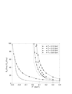
FIG. 1.: Leading Dirac amplitude for the pseudoscalar (shaded symbols) and scalar (open symbols) vertices, $E$ in Eqs. (26,53), evaluated at $(\vec{p}=0,\omega_{0})$ and plotted as function of $\vec{P}^{2}$ in the chiral limit; i.e., $E(\vec{p}=0,\omega_{0};\vec{P}^{2})$, for a range of temperature values. The bound state poles are evident in each case. (We use $\zeta=19\,$GeV throughout.)

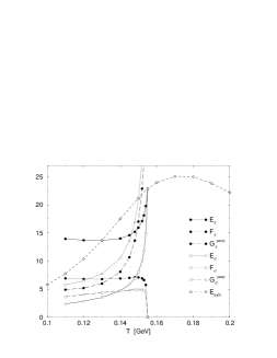
FIG. 2.: Dirac amplitudes characterising the $\hat{m}=0$ pseudoscalar and scalar bound states, evaluated at $(\vec{p}=0,\omega_{0})$. $G_{\pi}^{\perp}$, $G_{\pi}^{\|}$ and $F_{\sigma}$ behave similarly: as $T\to T_{c}^{-}$ their value at $(\vec{p}=0,\omega_{0})$ increases rapidly while the domain on which the functions are nonzero shrinks quickly. $E_{\rm sym}$ is the amplitude calculated in the chirally symmetric $B_{0}\equiv 0$ phase: above $T_{c}$, $E_{\pi}=E_{\sigma}=E_{\rm sym}$ while all other amplitudes vanish.

It is easy to understand this algebraically. The BSE is a set of coupled homogeneous equations for the Dirac amplitudes. Below $T_{c}$ each of the equations for the subleading Dirac amplitudes has an “inhomogeneity” whose magnitude is determined by $B_{0}$, the scalar piece of the quark self energy which is dynamically generated in the chiral limit. $B_{0}$ vanishes above $T_{c}$ eliminating the inhomogeneity and allowing a trivial, identically zero solution for each of these amplitudes. Additionally, with $B_{0}\equiv 0$ the kernels in the equations for the dominant pseudoscalar and scalar amplitudes are identical, and hence so are the solutions.

It follows from these results that the Goldberger-Treiman-like relation[27]

$$f_{\pi}^{0}E_{\pi}(p_{\omega_{k}};0)=B_{0}(p_{\omega_{k}})\,,$$ (44)

is satisfied for all $T$ only because both $f_{\pi}^{0}$ and $B_{0}(p_{\omega_{k}})$ are equivalent order parameters for chiral symmetry restoration. This possibility was overlooked in Ref. [36]. Further, above $T_{c}$, the other constraints on the chiral-limit pion Bethe-Salpeter amplitude derived in Ref. [27] from the axial-vector Ward-Takahashi identity are trivially satisfied.

Using the bound state amplitudes and dressed-quark propagators we calculate the matrix elements discussed in Sec. II. Their chiral limit $T$-dependence is depicted in Fig. 3. As indicated by Fig. 1, the pseudoscalar and scalar bound states are massive and degenerate above $T_{c}$.

Below $T_{c}$ the scalar meson residue in the scalar vertex, $r_{\sigma}$ in Eq. (37), is a little larger than the residue of the pseudoscalar meson in the pseudoscalar vertex, $r_{\pi}$ in Eq. (30). However, they are nonzero and equal above $T_{c}$, which is an algebraic consequence of $B_{0}\equiv 0$ and the vanishing of the subleading Dirac amplitudes. As a bona fide order parameter for chiral symmetry restoration

$$f_{\pi}\propto(1-T/T_{c})^{\beta}\,,\;T/T_{c}\mathrel{\hbox to0.0pt{\lower 4.0pt\hbox{\hskip 0.0pt$\sim$}\hss}\raise 1.0pt\hbox{$<$}}1\,,$$ (45)

where $\beta$ is the zero-external-field critical-exponent for chiral symmetry restoration ($\beta=1/2$ in rainbow-ladder models)[17]. $f_{\pi}=0$ and $r_{\pi}\neq 0$ for $T>T_{c}$ demonstrates that the pion disappears as a pole in the axial-vector vertex[36] but persists as a pole in the pseudoscalar vertex.

Our analysis yields

$$m_{\sigma}\propto(1-T/T_{c})^{\beta}\,,\;T/T_{c}\mathrel{\hbox to0.0pt{\lower 4.0pt\hbox{\hskip 0.0pt$\sim$}\hss}\raise 1.0pt\hbox{$<$}}1\,,$$ (46)

within numerical errors, which is evident in Fig. 3: $m_{\sigma}^{2}$ follows a linear trajectory in the vicinity of $T_{c}$. Such behaviour in the isoscalar-scalar channel might be anticipated because this channel has vacuum quantum numbers and hence the bound state is a strong interaction analogue of the electroweak Higgs boson[6].

$m_{\rm sym}^{2}$ in Fig. 3 is the mass obtained when the chirally symmetric solution of the quark DSE is used in the BSE. ($B_{0}\equiv 0$ is always a solution in the chiral limit.) For $T>T_{c}$, $m_{\rm sym}^{2}(T)$ is the unique meson mass-squared trajectory. However, for $T<T_{c}$, $m_{\rm sym}^{2}<0$; i.e., the solution of the BSE in the Wigner-Weyl phase exhibits a tachyonic solution (cf. the Nambu-Goldstone phase masses: $m_{\sigma}^{2}>m_{\pi}^{2}=0$). By analogy with the $\sigma$-model this tachyonic mass indicates the instability of the Wigner-Weyl phase below $T_{c}$. It translates into the statement that the pressure is not maximal in this phase.

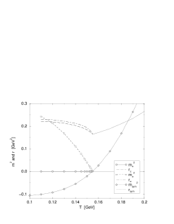
FIG. 3.: $\hat{m}=0$ results. Upper panel: $T$-dependence of the meson masses-squared and pole-residue matrix elements, Eqs. (30,31,37), along with the mass-squared: $m_{\rm sym}^{2}$, and residue: $r_{\rm sym}$, calculated in the chirally symmetric $B_{0}\equiv 0$ phase. For $T\leq T_{c}$, $m_{\rm sym}^{2}<0$, which is a signal of the instability of the chirally symmetric phase at low $T$. For $T>T_{c}$, $m_{\pi}^{2}=m_{\sigma}^{2}=m_{\rm sym}^{2}$. Lower panel: $T$-dependence of the masses and pion decay constant. $m_{\pi}=0$ within numerical error.

Figure 4 depicts the evolution of the (common) meson mass at large $T$. As expected in a gas of weakly interacting quarks and gluons

$$\frac{m_{\rm meson}}{2\,\omega_{0}}\to 1^{-}\,,$$ (47)

where $\omega_{0}=\pi T$ is a quark’s zeroth Matsubara frequency and “screening mass.”

B Nonzero light current-quark masses

It is straightforward to repeat the calculations of Sec. III A for nonzero current-quark masses where chiral symmetry restoration with increasing $T$ is exhibited as a crossover rather than a phase transition. The solutions of the inhomogeneous BSEs again exhibit a pole for all $T$ and we determine the bound state amplitudes from the associated homogeneous equations. Their $T$-dependence is characterised in Fig. 5, which shows that for $\hat{m}\neq 0$ they are locally identical for $T\mathrel{\hbox to0.0pt{\lower 4.0pt\hbox{\hskip 0.0pt$\sim$}\hss}\raise 1.0pt\hbox{$>$}}\frac{4}{3}T_{c}$.

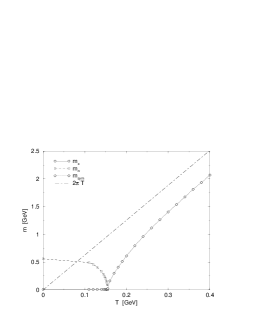
FIG. 4.: $T$-dependence of for large $T$ with $\hat{m}=0$, see Fig. 3. $m_{\pi}=m_{\sigma}$ for $T>T_{c}$ and $m/(2\pi T)\to 1^{-}$. This behaviour persists with $\hat{m}\neq 0$, however, providing an illustration requires significantly more computer time. (That is easier in a simpler model [10, 19].)

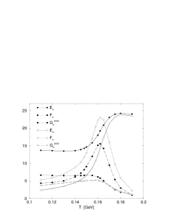
FIG. 5.: Dirac amplitudes characterising the $\hat{m}\neq 0$ pseudoscalar and scalar bound states, evaluated at $(\vec{p}=0,\omega_{0})$ and plotted as a function of temperature.

Figure 6 is the $\hat{m}\neq 0$ analogue of Fig. 3. That the transition has become a crossover is evident in the behaviour of $f_{\pi}$. The meson masses become indistinguishable at $T\sim 1.2\,T_{c}$, a little before the local equivalence is manifest in Fig. 5, which is unsurprising given that the mass is an integrated quantity. The small difference between $r_{\sigma}$ and $r_{\pi}$ below $T_{c}$ is again evident and they assume a common value at the same temperature as the masses.

Figure 7 illustrates the preservation of the axial-vector Ward-Takahashi identity via the mass formula of Eq. (33). The magnitude and $T$-dependence of both sides are equal within numerical errors above and below the crossover. $m_{R}(\zeta)\,r_{\pi}^{0}(\zeta)$ is the renormalisation point independent quantity that appears in the pion’s current algebra mass formula: $m_{R}(\zeta)\,r_{\pi}^{0}(\zeta)$ and $m_{R}(\zeta)\,r_{\pi}(\zeta)$ differ by $<5$% until $T>0.95\,T_{c}$. This comparison illustrates the $T$-domain on which the current algebra formula is valid and the analysis of Ref. [39]. It was noted in Ref. [17] that

$$r_{\pi}^{0}(\zeta)/f_{\pi}^{0}\propto(1-T/T_{c})^{-\beta}\,,\;T/T_{c}\mathrel{\hbox to0.0pt{\lower 4.0pt\hbox{\hskip 0.0pt$\sim$}\hss}\raise 1.0pt\hbox{$<$}}1\,,$$ (48)

which is qualitatively apparent from Figs. 3 and 7.

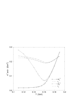
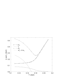
FIG. 6.: $T$-dependence of the meson masses and pole-residue matrix elements, Eqs. (30,31,37), for $\hat{m}\neq 0$.

C Triangle Diagrams

We also studied the matrix elements describing the two-body decays discussed in Sec. II D. With every element in the calculation only known numerically this too is a challenging numerical exercise, which we simplified by a judicious choice of the external momenta.

The chiral limit isoscalar-scalar-$\pi\pi$ coupling and width obtained from Eq. (59) are depicted in Fig. 8, which indicates that both vanish at $T_{c}$ in the chiral limit. Again this can be traced to $B_{0}\to 0$. For $\hat{m}\neq 0$, the coupling reflects the crossover. However, that is moot because the width vanishes just below $T_{c}$ where the isoscalar-scalar meson mass falls below $2m_{\pi}$ and the phase space factor vanishes (see the lower panel of Fig. 6).

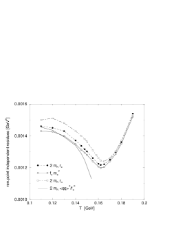
FIG. 7.: $T$-dependence of the residue of the pion pole in the axial-vector vertex, $f_{\pi}m_{\pi}^{2}$, and in the pseudoscalar vertex, $2\,m_{R}(\zeta)\,r_{\pi}(\zeta)$. They are equal within numerical errors as required by the axial-vector Ward-Takahashi identity. For comparison we also plot $2\,m_{R}(\zeta)\,r_{\pi}^{0}(\zeta)$ and the residue of the scalar meson pole in the scalar vertex, $2\,m_{R}(\zeta)\,r_{\sigma}(\zeta)$.

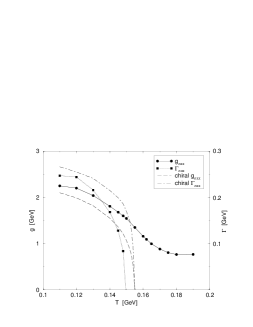
FIG. 8.: $T$-dependence of the isoscalar-scalar-$\pi\pi$ coupling and width, both in the chiral limit and for realistic light current-quark masses. The phase space factor $(1-(2m_{\pi}/m_{\sigma})^{2})^{1/2}$ is $\theta(T_{c}-T)$ in the chiral limit but nontrivial for $\hat{m}\neq 0$, vanishing at $T\approx 0.98\,T_{c}$; i.e., this decay channel closes at a temperature just $2$% less-than $T_{c}$.

The $T$-dependence of the $\pi^{0}\gamma\gamma$ coupling, which saturates the Abelian anomaly at $T=0$, is calculated from Eqs. (65,68) and depicted along with the width in Fig. 9. In the chiral limit the width is identically zero because $m_{\pi}=0$ and the interesting quantity is: ${\cal T}(0)=g^{0}_{\pi^{0}\gamma\gamma}/f_{\pi}^{0}$. Clear in the figure is that ${\cal T}(0)$ vanishes at $T_{c}$. It vanishes with a mean field critical exponent, as is most easily inferred from Fig. 10. (An accurate calculation is possible because Eq. (44) obviates the need for a solution of the BSE.) Thus, in the chiral limit, the coupling to the dominant decay channel closes for both charged and neutral pions. These features were anticipated in Ref. [40]. Further, as is evident in Fig. 10, our calculated ${\cal T}(0)$ is monotonically decreasing with $T$, supporting the perturbative O($T^{2}/f_{\pi}^{2})$ analysis in Ref. [41].

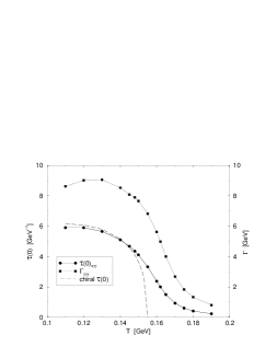
FIG. 9.: $T$-dependence of the coupling ${\cal T}(0)$ in Eq. (68) and the $\pi^{0}\to\gamma\gamma$ width.

For $\hat{m}\neq 0$ both the coupling: $g_{\pi^{0}\gamma\gamma}/f_{\pi}$, and the width exhibit the crossover with a slight enhancement in the width as $T\to T_{c}$ due to the increase in $m_{\pi}$. There are similarities between these results and those of Ref. [42] although the $T$-dependence herein is much weaker because our pion mass approaches twice the $T\neq 0$ free-quark screening-mass from below, never reaching it, Eq. (47); i.e., the continuum threshold is not crossed.

IV Summary and Conclusion

We employed a renormalisation group improved rainbow-ladder truncation of the quark Dyson-Schwinger equation, and pseudoscalar and scalar Bethe-Salpeter equations to estimate the $T$-dependence of a range of properties that characterise correlations in these channels. The rainbow-ladder truncation is quantitatively reliable in the pseudoscalar channel. However, that is not certain in the scalar channel where the cancellations that assist in the pseudoscalar channel are not apparent. Nevertheless, we anticipate that many of the features we exposed in the scalar channel are qualitatively correct.

The solutions of the inhomogeneous Bethe-Salpeter equation (BSE) exhibit poles at all $T$, both above and below the critical temperature, and in the chiral limit and for realistic light current-quark masses. We use the associated homogeneous BSEs to determine the masses, which correspond to the screening masses determined in simulations of lattice-QCD, and find $m_{\sigma,\pi}\to 2\pi T$ as $T\to\infty$.

FIG. 10.: $T$-dependence of $g^{0}_{\pi\gamma\gamma}=f_{\pi}^{0}{\cal T}(0)$. Within numerical error, $g^{0}_{\pi\gamma\gamma}\propto(1-T/T_{c})$. Near $T_{c}$, $f_{\pi}\propto(1-T/T_{c})^{1/2}$ because our model has mean field critical exponents and hence ${\cal T}(0)\propto(1-T/T_{c})^{1/2}$.

The BSE solutions indicate a local equivalence between the isovector-scalar and -pseudoscalar correlations above the chiral restoration transition/crossover; i.e., the scalar functions characterising the bound state amplitudes are identical, and from this follows equality of the masses and many of the matrix elements. Further, the axial-vector Ward-Takahashi identity and the pseudoscalar mass formula that is its corollary are valid both above and below the crossover.

For realistic light current-quark masses the isoscalar-scalar meson mass does not fall below $2m_{\pi}$ until very near the transition temperature. Hence this dominant decay channel remains open almost until the phase boundary is crossed. Once it is crossed, however, only electroweak decay channels are open. In the chiral limit the anomalous two-photon coupling constant vanishes at $T_{c}$ just as does $f_{\pi}$, the coupling that determines the strength of the leptonic charged pion decay. For realistic masses, however, the widths for the leptonic charged pion mode and two-photon $\pi^{0}$ mode remain significant in the vicinity of the crossover.

The construction of a DSE-BSE truncation that allows for an improved description of the scalar channel at $T=0$ would provide the foundation for a significant improvement of our analysis. Employing an Ansatz for the kernel of the quark DSE whose infrared form exhibits some $T$-dependence, perhaps constrained by lattice simulations of the string tension[1], may also be interesting. However, given the results of Refs. [17, 43], we do not expect such a modification to have a significant qualitative impact. In the absence of such improvements we nevertheless expect the local equivalence we have elucidated to be exhibited by all isovector chiral partners in the strong interaction spectrum. However, the explicit demonstration of this is difficult; e.g., in the $\rho$-$a_{1}$ complex the bound state amplitudes have eight independent amplitudes even at $T=0$ compared with the four in the pseudoscalar and scalar amplitudes at $T\neq 0$.

Collected Formulae

1 Scalar Vertex

The inhomogeneous ladder-like Bethe-Salpeter equation for the zeroth Matsubara mode of the $0^{++}$ vertex is

$$\Gamma_{\rm s}^{\alpha}(p_{\omega_{k}};P_{0};\zeta)=Z_{4}\,\frac{1}{2}\tau^{\alpha}\mbox{\boldmath$1$}$$ (49)

$$-\int_{l,q}^{\bar{\Lambda}}\,\frac{4}{3}\,g^{2}D_{\mu\nu}(p_{\omega_{k}}-q_{\omega_{l}})$$ (50)

$$\times \gamma_{\mu}S(q_{\omega_{l}}^{+})\,\Gamma_{\rm s}^{i}(q_{\omega_{l}};P_{\Omega_{n}};\zeta)\,S(q_{\omega_{l}}^{-})\,\gamma_{\nu}\,,$$ (51)

where $\alpha=0,1,2,3$ with $\tau^{0}={\rm diag}(1,1)$. (NB: In this truncation the isoscalar and isovector states are degenerate, which exemplifies our observation that the ladder-like truncation is accurate for vector mesons but requires improvement before it is quantitatively reliable in the $0^{++}$ sector.) The solution has the form

$$\Gamma_{\rm s}^{i}(p_{\omega_{k}};\vec{P})=\frac{1}{2}\tau^{\alpha}\,\mbox{\boldmath$1$}\,\left[E_{\rm s}(p_{\omega_{k}};\vec{P})+i\vec{\gamma}\cdot\vec{p}\,G^{\|}_{\rm s}(p_{\omega_{k}};\vec{P})\right.$$ (52)

$$+ \left.i\gamma_{4}\omega_{k}\,G^{\perp}_{\rm s}(p_{\omega_{k}};\vec{P})+i\vec{\gamma}\cdot\vec{P}\,\vec{p}\cdot\vec{P}\,F_{\rm s}(p_{\omega_{k}};\vec{P})\right]\,.$$ (53)

(NB: Here the requirement that the neutral mesons be charge conjugation eigenstates shifts the $\vec{p}\cdot\vec{P}$ term cf. the $0^{-+}$ amplitude.)

The scalar functions in Eq.(51) exhibit a simple pole at $\vec{P}^{2}+m_{\sigma}^{2}=0$:

$$\Gamma_{\rm s}^{i}(p_{\omega_{k}};\vec{P})=\frac{r_{\sigma}(\zeta)}{\vec{P}^{2}+m_{\sigma}^{2}}\,\Gamma_{\sigma}^{i}(p_{\omega_{k}};\vec{P})+{\rm regular}\,,$$ (54)

where $\Gamma_{\sigma}^{i}(p_{\omega_{k}};\vec{P})$ is the canonically normalised, $0^{++}$ bound state Bethe-Salpeter amplitude:

$$2\delta^{\alpha\beta}\vec{P}={\rm tr}\,\int_{l,q}^{\bar{\Lambda}}\,\left\{\Gamma_{\sigma}^{\alpha}(q_{\omega_{l}};-\vec{P})\,\frac{\partial S(q_{\omega_{l}}^{+})}{\partial\vec{P}}\Gamma_{\sigma}^{\beta}(q_{\omega_{l}};\vec{P})\,S(q_{\omega_{l}}^{-})\right.$$ (56)

$$+\left.\left.\Gamma_{\sigma}^{\alpha}(q_{\omega_{l}};-\vec{P})\,S(q_{\omega_{l}}^{+})\Gamma_{\sigma}^{\beta}(q_{\omega_{l}};\vec{P})\,\frac{\partial S(q_{\omega_{l}}^{-})}{\partial\vec{P}}\right\}\right|_{\vec{P}^{2}=-m_{\rm s}^{2}}\!\!\!.$$

The dressed-quark propagator and canonically normalised Bethe-Salpeter amplitudes make possible the definition of the impulse approximation to the isoscalar-scalar-$\pi\pi$ matrix element: $\vec{p_{1}}^{2}=-m_{\pi}^{2}=\vec{p_{2}}^{2}$, $(\vec{p}=\vec{p_{1}}+\vec{p_{2}})^{2}=-m_{\sigma}^{2}$,

$$g_{\sigma\pi\pi}:=\langle\pi(\vec{p_{1}})\pi(\vec{p_{2}})|\sigma(\vec{p})\rangle=$$ (59)

$$2N_{c}{\rm tr}_{D}\int_{l,q}^{\bar{\Lambda}}\,\Gamma_{\sigma}(k_{\omega_{l}};\vec{p})\,S_{u}(k_{++})$$

$$\times i\Gamma_{\pi}(k_{0+};-\vec{p_{1}})\,S_{u}(k_{+-})\,i\Gamma_{\pi}(k_{-0};-\vec{p_{2}})\,S_{u}(k_{--})\,,$$

$k_{\alpha\beta}=k_{\omega_{l}}+(\alpha/2)\vec{p_{1}}+(\beta/2)\vec{p_{2}}$, with only the trace over Dirac indices remaining.

2 Neutral Pion Decay

An efficacious Ansatz for the dressed-quark-photon coupling at $T=0$ is[32, 33]:

$$i\Gamma_{\mu}(\ell_{1},\ell_{2})=i\Sigma_{A}(\ell_{1}^{2},\ell_{2}^{2})\,\gamma_{\mu}$$ (63)

$$+(\ell_{1}+\ell_{2})_{\mu}\,\left[\mbox{$\frac{1}{2}$}i\gamma\cdot(\ell_{1}+\ell_{2})\,\Delta_{A}(\ell_{1}^{2},\ell_{2}^{2})+\Delta_{B}(\ell_{1}^{2},\ell_{2}^{2})\right]\,;$$

$$\Sigma_{F}(\ell_{1}^{2},\ell_{2}^{2})=\mbox{$\frac{1}{2}$}\,[F(\ell_{1}^{2})+F(\ell_{2}^{2})]\,,$$

$$\Delta_{F}(\ell_{1}^{2},\ell_{2}^{2})=\frac{F(\ell_{1}^{2})-F(\ell_{2}^{2})}{\ell_{1}^{2}-\ell_{2}^{2}}\,,$$

where $F=A,B$; i.e., the scalar functions in the dressed-quark propagator: $S^{-1}(p)=i\gamma\cdot pA(p^{2})+B(p^{2})$, so that this model is completely determined by $S(p)$. Improvements of this Ansatz, such as those canvassed in Ref. [33], do not have a qualitatively significant effect in the present context.

The dressed-quark-photon vertex is a necessary element in the calculation of the impulse approximation to the $\pi^{0}\to\gamma\gamma$ amplitude. At $T=0$ the anomalous contribution to the divergence of the axial-vector vertex is saturated by the pseudoscalar piece of the pion Bethe-Salpeter amplitude[34]

$$\hat{T}_{\mu\nu}(k_{1},k_{2})={\rm tr}\int_{l,q}^{\bar{\Lambda}}\,S(q_{1})\,\gamma_{5}\tau^{3}iE_{\pi}(\hat{q};-P)\,$$ (64)

$$\times S(q_{2})\,i{\cal Q}\Gamma_{\mu}(q_{2},q_{12})\,S(q_{12})\,i{\cal Q}\Gamma_{\nu}(q_{12},q_{1})\,,$$ (65)

where ${\cal Q}={\rm diag}(2/3,-1/3)$ and herein $k_{1}=(\vec{k}_{1},0)$, $k_{2}=(\vec{k}_{2},0)$, $P=k_{1}+k_{2}$, $q_{1}=q_{\omega_{l}}-k_{1}$, $q_{2}=q_{\omega_{l}}+k_{2}$, $\hat{q}=\frac{1}{2}(q_{1}+q_{2})$, $q_{12}=q_{\omega_{l}}-k_{1}+k_{2}$. Using Eq. (63) to evaluate Eq. (65) for real photons at $T=0$ one obtains

$$\hat{T}_{\mu\nu}(k_{1},k_{2})=\frac{\alpha_{\rm em}}{\pi}\,\epsilon_{\mu\nu\rho\sigma}\,k_{1\rho}\,k_{2\sigma}\,{\cal T}(0)\,,$$ (66)

with in the chiral limit[30]

$$f_{\pi}^{0}\,{\cal T}(0):=g_{\pi^{0}\gamma\gamma}=1/2\,.$$ (67)

At nonzero $T$ the tensor structure of Eq. (66) survives to the extent that, with our choice of $k_{1}$, $k_{2}$, it ensures one of the photons is longitudinal (a plasmon) and the other transverse. In this case we determine the $T$-dependence using

$$\hat{T}_{i4}(k_{1},k_{2})=\frac{\alpha_{\rm em}}{\pi}\,(\vec{k_{1}}\times\vec{k_{2}})_{i}\,{\cal T}(0)$$ (68)

and a generalisation of Eq. (63) to nonzero $T$:

$$i\vec{\Gamma}(q_{\omega_{l_{1}}},q_{\omega_{l_{2}}})=\Sigma_{A}(q_{\omega_{l_{1}}}^{2},q_{\omega_{l_{2}}}^{2})\,i\vec{\gamma}$$ (69)

$$+ (\vec{q}_{1}+\vec{q}_{2})\,[\frac{1}{2}\,iG(q_{\omega_{l_{1}}},q_{\omega_{l_{2}}})+\Delta_{B}(q_{\omega_{l_{1}}}^{2},q_{\omega_{l_{2}}}^{2})],$$ (70)

$$i\Gamma_{4}(q_{\omega_{l_{1}}},q_{\omega_{l_{2}}})=\Sigma_{C}(q_{\omega_{l_{1}}}^{2},q_{\omega_{l_{2}}}^{2})\,i\gamma_{4}$$ (72)

$$+(\omega_{l_{1}}+\omega_{l_{2}})\,[\frac{1}{2}\,iG(q_{\omega_{l_{1}}},q_{\omega_{l_{2}}})+\Delta_{B}(q_{\omega_{l_{1}}}^{2},q_{\omega_{l_{2}}}^{2})],$$

$$G(q_{\omega_{l_{1}}},q_{\omega_{l_{2}}})=\vec{\gamma}\cdot(\vec{q}_{1}+\vec{q}_{2})\Delta_{A}(q_{\omega_{l_{1}}}^{2},q_{\omega_{l_{2}}}^{2})$$ (74)

$$+\gamma_{4}(\omega_{l_{1}}+\omega_{l_{2}})\Delta_{C}(q_{\omega_{l_{1}}}^{2},q_{\omega_{l_{2}}}^{2}),$$

which satisfies the vector Ward-Takahashi identity

$$(q_{\omega_{l_{1}}}-q_{\omega_{l_{2}}})_{\mu}\,i\Gamma_{\mu}(q_{\omega_{l_{1}}},q_{\omega_{l_{2}}})=S^{-1}(q_{\omega_{l_{1}}})-S^{-1}(q_{\omega_{l_{2}}}).$$ (75)

REFERENCES

- [1] E. Laermann, Fiz. Élem. Chastits At. Yadra 30, 720 (1999) (Phys. Part. Nucl. 30, 304 (1999)).
- [2] QCD Phase Transitions, Proceedings of the XXVth International Workshop on Gross Properties of Nuclei and Nuclear Excitations, Hirschegg, Austria, 1997, edited by H. Feldmeier, J. Knoll, W. Norenberg and J. Wambach (GSI, Darmstadt, 1997).
- [3] Understanding Deconfinement in QCD, Proceedings of the International Workshop on Understanding Deconfinement in QCD, Trento, Italy, 1999, edited by D. Blaschke, F. Karsch and C.D. Roberts (World Scientific, Singapore, 2000).
- [4] M. Boglione and M.R. Pennington, Eur. Phys. J. C 9, 11 (1999).
- [5] M.R. Pennington, “Riddle of the scalars: Where is the ?,” hep-ph/9905241.
- [6] M.R. Pennington, “Low Energy Hadron Physics,” hep-ph/0001183.
- [7] J.C.R. Bloch, M.A. Ivanov, T. Mizutani, C.D. Roberts and S.M. Schmidt, “ and a light scalar meson,” nucl-th/9910029.
- [8] C.D. Roberts and A.G. Williams, Prog. Part. Nucl. Phys. 33, 477 (1994); C.D. Roberts, “Nonperturbative QCD with modern tools,” in Proceedings of the 11th Physics Summer School: Frontiers in Nuclear Physics, edited by S. Kuyucak (World Scientific, Singapore, 1999) p. 212.
- [9] C.D. Roberts, Fiz. Élem. Chastits At. Yadra 30, 537 (1999) (Phys. Part. Nucl. 30, 223 (1999)).
- [10] D. Blaschke and P.C. Tandy, “Mesonic correlations and quark deconfinement,” in Ref. [3], p. 218.
- [11] J.C.R. Bloch, C.D. Roberts and S.M. Schmidt, Phys. Rev. C 60, 065208 (1999).
- [12] J. Engels, R. Joswig, F. Karsch, E. Laermann, M. Lutgemeier and B. Petersson, Phys. Lett. B 396, 210 (1997).
- [13] D. Blaschke, C.D. Roberts and S.M. Schmidt, Phys. Lett. B 425, 232 (1998).
- [14] P. Maris and C.D. Roberts, Phys. Rev. C 56, 3369 (1997).
- [15] L.S. Kisslinger, M. Aw, A. Harey and O. Linsuain, Phys. Rev. C 60, 065204 (1999).
- [16] J.I. Skullerud and A.G. Williams, “The quark propagator in momentum space,” hep-lat/9909142.
- [17] A. Höll, P. Maris and C.D. Roberts, Phys. Rev. C59, 1751 (1999).
- [18] P. Maris, C.D. Roberts and S.M. Schmidt, Phys. Rev. C 57, 2821 (1998).
- [19] D. Blaschke, G. Burau, Yu.L. Kalinovsky, P. Maris and P.C. Tandy, “Finite correlations and quark deconfinement,” preprint nos. MPG-VT-UR 192/99, KSUCNR-101-00.
- [20] P. Maris and P.C. Tandy, “The quark photon vertex and the pion charge radius,” nucl-th/9910033.
- [21] J.C.R. Bloch, C.D. Roberts and S.M. Schmidt, “Selected nucleon form factors and a composite scalar diquark,” nucl-th/9911068.
- [22] F.T. Hawes, P. Maris and C.D. Roberts, Phys. Lett. B 440, 353 (1998).
- [23] H.J. Munczek and A.M. Nemirovsky, Phys. Rev. D 28, 181 (1983).
- [24] P. Jain and H.J. Munczek, Phys. Rev. D 48, 5403 (1993).
- [25] A. Bender, C.D. Roberts and L. v. Smekal, Phys. Lett. B 380, 7 (1996).
- [26] P. Maris and P C. Tandy, Phys. Rev. C 60, 055214 (1999).
- [27] P. Maris, C.D. Roberts and P.C. Tandy, Phys. Lett. B 420, 267 (1998).
- [28] C.D. Roberts, in Quark Confinement and the Hadron Spectrum II, edited by N. Brambilla and G. M. Prosperi (World Scientific, Singapore, 1997), pp. 224-230.
- [29] M.R. Frank and T. Meissner, Phys. Rev. C 57, 345 (1998); L. v. Smekal, A. Mecke and R. Alkofer, “A dynamical mass from an infrared enhanced gluon exchange,” hep-ph/9707210.
- [30] C.D. Roberts, Nucl. Phys. A 605, 475 (1996).
- [31] C.D. Roberts, Fizika B8, 285 (1999); P.C. Tandy, ibid, 295; D. Klabucar and D. Kekez, Fizika ibid, 303.
- [32] J.S. Ball and T. Chiu, Phys. Rev. D 22, 2542 (1980).
- [33] A. Bashir, A. Kizilersu and M.R. Pennington, Phys. Rev. D 57, 1242 (1998); and references therein.
- [34] P. Maris and C.D. Roberts, Phys. Rev. C 58, 3659 (1998).
- [35] Particle Data Group (C. Caso et al.), Eur. Phys. J. C 3, 1 (1998).
- [36] A. Bender, D. Blaschke, Yu.L. Kalinovsky and C.D. Roberts, Phys. Rev. Lett. 77, 3724 (1996).
- [37] C.J. Burden, L. Qian, C.D. Roberts, P.C. Tandy and M.J. Thomson, Phys. Rev. C 55, 2649 (1997).
- [38] L.C.L. Hollenberg, C.D. Roberts and B.H.J. McKellar, Phys. Rev. C 46, 2057 (1992); K.L. Mitchell and P.C. Tandy, Phys. Rev. C 55, 1477 (1997); M.A. Pichowsky, S. Walawalkar and S. Capstick, Phys. Rev. D 60, 054030 (1999).
- [39] S.M. Schmidt, D. Blaschke and Yu.L. Kalinovsky, Z. Phys. C 66, 485 (1995).
- [40] R.D. Pisarski, Phys. Rev. Lett. 76, 3084 (1996).
- [41] R.D. Pisarski and M. Tytgat, Phys. Rev. D 56, 7077 (1997).
- [42] D. Blaschke, Yu.L. Kalinovsky, P. Petrow, S.M. Schmidt, M. Jaminon and B. Van den Bossche, Nucl. Phys. A 592, 561 (1995).
- [43] R. Alkofer, P.A. Amundsen and K. Langfeld, Z. Phys. C42, 199 (1989).