UG-DFM-1/2000

nucl-th/0001060

Deeply bound levels in kaonic atoms.

A. Baca, C. García-Recio and J. Nieves
Departamento de Física Moderna, Universidad de Granada, E-18071 Granada, Spain.

Using a microscopic antikaon-nucleus optical potential recently developed by Ramos and Oset [10] from a chiral model, we calculate strong interaction energy shifts and widths for $K^{-}$ atoms. This purely theoretical potential gives an acceptable description of the measured data ($\chi^{2}/{\rm num.data}=3.8$), though it turns out to be less attractive than what can be inferred from the existing kaon atomic data. We also use a modified potential, obtained by adding to the latter theoretical one a $s$-wave term which is fitted to known experimental kaonic data ($\chi^{2}/{\rm degree~{}of~{}freedom}=1.6$), to predict deeply bound $K^{-}$ atomic levels, not yet detected. This improved potential predicts, in general, states even narrower than those recently reported by Friedman and Gal [9]. This reinforces the idea that these deeply atomic states can be detected and resolved by using suitable nuclear reactions. Besides, we also study $K^{-}$ and $\bar{K}^{0}$ nuclear bound states and compute binding energies and widths, for both species of antikaons, in ¹²C, ⁴⁰Ca and ²⁰⁸Pb. Despite of restricting our study only to potentials obtained from best fits to the known kaonic atom data, the dynamics of these nuclear bound states depends dramatically on the particular optical potential used.

PACS: 13.75.Jz, 21.65.+f, 36.10.-k, 36.10.Gv, 11.30.Rd
Keywords: kaonic atoms and nuclei, deeply bound states, chiral symmetry .

1 Introduction

Strong interaction shifts and widths of bound levels of hadronic atoms provide valuable information on the hadron-nucleus interaction at threshold [1]. We call deeply bound hadronic states those that cannot be detected by means of spectroscopic tools ($i.e.$ analyzing the emitted $X-$rays when the hadron decays from one atomic level to another one in the electromagnetic cascade). This happens for low-lying levels where the overlap between the hadron wave-function and the nucleus is appreciable, and as a consequence the width due to strong interaction of the hadron with the nucleus is much larger than the electromagnetic width of the level. In these circumstances, the emission of $X-$rays is highly suppressed as compared to the hadron absorption by the nucleus. Indeed, the total decay width of the last observable level, using $X-$ray spectroscopy techniques, is two or three orders of magnitude larger than the upper one. Thus, the width of these deeply bound states are expected to be very large. If the half-width of a given level is equal or larger than the separation to the next level, then that state cannot be resolved. So only narrow deeply bound states can be resolved and detected. It is out of any doubt that the precise experimental determination of binding energies and widths of these states would provide a valuable insight into the complex dynamics of the antikaon-nucleon and antikaon-nucleus systems. Similar studies have been carried out for the pion case, where narrow deeply bound pionic atom states were predicted [2]-[4], and have been recently detected using nuclear reactions  [5].

By using $X-$ray spectroscopy techniques, energy shifts and widths of kaonic atoms levels have been measured through the whole periodic table. A compilation of data can be found in Refs. [1] and [6]. Some $K^{-}-$nucleus optical potentials have been successfully fitted to experimental data [1],  [6]-[8] and recently used by Friedman and Gal to predict the existence of narrow deeply bound levels in kaonic atoms [9]. These authors find that the $K^{-}$ deeply bound atomic levels are generally narrow, with widths ranging for $50$ to $1500$ KeV over the entire periodic table, and are not very sensitive to the different density dependence of the $K^{-}-$nucleus optical potentials that were used. Besides, they also note that, due to the strong attraction of the antikaon-nucleus optical potential, there must exist nuclear kaonic bound levels, deeper than the atomic states, which, in contrast, are expected to be very sensitive to the density dependence of the different optical potentials.

From the microscopical point of view, recently Ramos and Oset [10] have developed an optical potential for the $K^{-}$ meson in nuclear matter in a self-consistent microscopic manner. This approach uses a $s$-wave $\bar{K}N$ interaction obtained by solving a coupled-channel Lippmann-Schwinger equation, in the $S=-1$ strangeness sector, with a kernel determined by the lowest-order meson-baryon chiral Lagrangian [11]. Though, a three-momentum cut-off, which breaks manifest Lorentz covariance, is introduced to regularize the chiral loops, the approach followed by the authors of [11] restores exact unitarity and it is able to accommodate the resonance $\Lambda(1405)$. Self-consistency turns out to be a crucial ingredient to derive the $K^{-}-$nucleus potential in Ref. [10] and leads to an optical potential considerably more shallow than those found in Refs.  [1],  [6]-[8]. This was firstly pointed out by Lutz in Ref. [16], where however, $\eta$Y channels were not included when solving the coupled-channel Lippmann-Schwinger equation for the $\bar{K}N$ interaction, in the free space. Another recent work [17], where the medium modifications of antikaons in dense matter are studied in a coupled channel calculation, for scenarios more closely related to the environment encountered in heavy-ion collisions, also confirms the importance of self-consistency to find a similarly shallow potential. The depth of the real potential in the interior of nuclei is a topic of current interest in connection with possible kaon condensation in astrophysical scenarios [18].

In this work we have three aims. First, to see how this new microscopical optical potential [10], hereafter called $V_{\rm opt}^{(1)}$, describes the known kaonic atom levels and, if possible, quantify its quality. Second, taking $V_{\rm opt}^{(1)}$ as starting point, without modification and also adding to it a phenomenological part fitted to the kaonic atom data, to give predictions of deeply bound kaonic atoms levels and compare them with previous predictions. Third, to calculate the binding energies and widths of the nuclear kaonic states for both $K^{-}$ and $\bar{K}^{0}$.

In Ref. [19], some results obtained with the potential $V_{\rm opt}^{(1)}$ have been very recently reported. Here, we try to quantify the deficiencies of this interaction and give more reliable predictions for states not yet observed, thanks to the use of a potential which describes better the measured data. As a matter of example, the nuclear $K^{-}$ widths predicted in Ref. [19] are about a factor two bigger than those obtained in this work. Thus, all nuclear states given in Ref. [19] do have overlap with the continuum, their meaning thus being unclear. Furthermore, we also present here calculations for the $\bar{K}^{0}-$nuclear states, not mentioned in Ref. [19] at all.

The set of experimental data we have used through this work contains 63 energy shifts and widths of kaonic atom levels. Those are all data compiled in Refs. [1] and [6] except for the $3d$ energy shift in Helium and the $6h$ energy shift in Ytterbium . We define the strong shift for each level by means of

$$\varepsilon=B_{c}-B$$ (1)

where $B$ and $B_{c}$ are the total and the purely electromagnetic binding energies, respectively. Both of them are negative, and thus a negative (positive) energy shift means that the net effect of the strong potential is repulsive (attractive). To compute de $K^{-}-$nucleus bound states, we solve the Klein-Gordon equation (KGE) with an electromagnetic, $V_{c}$, and a strong optical, $V_{\rm opt}$, potentials, it reads:

$$\left(-\nabla^{2}+\mu^{2}+2\mu V_{\rm opt}(r)\right)\Psi=\left(E-V_{c}(r)\right)^{2}\Psi$$

where $\mu$ is the $K^{-}-$nucleus reduced mass, the real part of $E$ is the total meson energy, including its mass, and the imaginary part of $E$, changed of sign, is the half-width $\Gamma/2$ of the state. Different models for $V_{\rm opt}$ will be discussed in detail in the next section, whereas for $V_{c}(r)$ we use the Coulomb interaction taking exactly the finite-size distribution of the nucleus and adding to it the vacuum-polarization corrections [20].

Both the minimization numerical algorithm and the one used to solve the KGE in coordinate space, have been extensively tested in the similar problem of pionic atoms [4].

2 Experimental kaonic atom data and the optical potentials

The $K^{-}-$nucleus optical potential for kaonic atoms, $V_{\rm opt}$, is related to the $K^{-}-$self-energy, $\Pi_{K^{-}},$ inside of a nuclear medium. This relation reads:

$$2\mu V_{\rm opt}(r) = \Pi_{K^{-}}(q_{0}=m_{K},\vec{q}=0,\rho_{p}(r),\rho_{n}(r)),$$ (2)

where the $K^{-}-$self-energy is evaluated at threshold, and $\rho_{p(n)}(r)$ is the proton (neutron) density. Neglecting isovector effects, as we will do in the rest of the paper, the optical potential only depends on $\rho(r)=\rho_{p}(r)+\rho_{n}(r)$. Charge densities are taken from [21]. For each nucleus, we take the neutron matter density approximately equal to the charge one, though we consider small changes, inspired by Hartree-Fock calculations with the DME (density-matrix expansion) [22]. In Table 1 we compile the densities used through this work. However charge (neutron matter) densities do not correspond to proton (neutron) ones because of the finite size of the proton (neutron). We take that into account following the lines of Ref. [4].

Nucleus	$R_{p}$ [fm]	$R_{n}$[fm]	$a$ [fm]∗
7LiMHO	1.770	1.770	0.327
9BeMHO	1.791	1.791	0.611
10BMHO	1.710	1.710	0.837
11BMHO	1.690	1.690	0.811
12CMHO	1.672	1.672	1.150
16OMHO	1.833	1.833	1.544
24Mg	2.980	2.930	0.551
27Al	2.840	2.840	0.569
28Si	2.930	2.860	0.569
31P	3.078	3.078	0.569
32S	3.165	3.079	0.569
35Cl	3.395	3.395	0.569
40Ca	3.51	3.43	0.563
59Co	4.080	4.180	0.569
58Ni	4.090	4.140	0.569
63Cu	4.200	4.296	0.569
108Ag	5.300	5.500	0.532
112Cd	5.380	5.580	0.532
115In	5.357	5.557	0.563
118Sn	5.300	5.550	0.583
165Ho	6.180	6.430	0.570
173Yb	6.280	6.530	0.610
natTa	6.380	6.630	0.640
208Pb	6.624	6.890	0.549
238U	6.805	7.055	0.605

Table 1: Charge ($R_{p},a$) and neutron matter ($R_{n},a$) density parameters. For light nuclei ($A\leq 16$) we use a modified harmonic oscillator (MHO) whereas for heavier nuclei ($A>16$) a two-parameter Fermi distribution was used. (*) The parameter $a$ is dimensionless for the MHO density form.

As we mentioned in the introduction, the authors of Ref. [10] have developed an optical potential for the $K^{-}$ meson in nuclear matter in a self-consistent microscopic manner. It is based on their previous work [11] on the $s$-wave meson-baryon dynamics in the $S=-1$ strangeness sector. There, and starting from the lowest-order meson-baryon chiral Lagrangian, a non-perturbative resummation of the bubbles in the $s$-channel is performed. Such a resummation leads to an exact restoration of unitarity. The model reproduces successfully the $\Lambda(1405)$ resonance and the $K^{-}p\to K^{-}p,\bar{K}^{0}n,\pi^{0}\Lambda,\pi^{0}\Sigma,\pi^{+}\Sigma^{-},\pi^{-}\Sigma^{+}$ cross sections at low energies. The results in nuclear matter are translated to finite nuclei by means of the local density approximation, which turns out to be exact for zero-range interactions [23], which is the case of the $s$-wave part of the $K^{-}-$nucleus optical potential for kaonic atoms.

		Lower level energy shifts $\varepsilon$ [KeV]
Nucleus	$nl$	(1)	(1m)	(2)	(2DD)	Exp.
7Li	2p	$-$0.010	$-$0.003	$-$0.007	$-$0.015	0.002 $\pm$ 0.026
9Be	2p	$-$0.068	$-$0.039	$-$0.060	$-$0.077	$-$0.079 $\pm$ 0.021
10B	2p	$-$0.217	$-$0.159	$-$0.198	$-$0.195	$-$0.208 $\pm$ 0.035
11B	2p	$-$0.235	$-$0.199	$-$0.209	$-$0.182	$-$0.167 $\pm$ 0.035
12C	2p	$-$0.623	$-$0.630	$-$0.556	$-$0.481	$-$0.590 $\pm$ 0.080
16O	3d	$-$0.001	0.0001	$-$0.0004	$-$0.001	$-$0.025 $\pm$ 0.018
24Mg	3d	$-$0.057	$-$0.028	$-$0.034	$-$0.036	$-$0.027 $\pm$ 0.015
27Al	3d	$-$0.109	$-$0.069	$-$0.064	$-$0.076	$-$0.080 $\pm$ 0.013
28Si	3d	$-$0.192	$-$0.135	$-$0.118	$-$0.145	$-$0.139 $\pm$ 0.014
31P	3d	$-$0.379	$-$0.323	$-$0.253	$-$0.322	$-$0.330 $\pm$ 0.080
32S	3d	$-$0.606	$-$0.548	$-$0.418	$-$0.537	$-$0.494 $\pm$ 0.038
35Cl	3d	$-$1.14	$-$1.11	$-$0.848	$-$1.05	$-$1.00 $\pm$ 0.17
59Co	4f	$-$0.185	$-$0.14	$-$0.105	$-$0.152	$-$0.099 $\pm$ 0.106
58Ni	4f	$-$0.239	$-$0.185	$-$0.137	$-$0.197	$-$0.223 $\pm$ 0.042
63Cu	4f	$-$0.384	$-$0.335	$-$0.239	$-$0.329	$-$0.370 $\pm$ 0.047
108Ag	5g	$-$0.39	$-$0.354	$-$0.263	$-$0.342	$-$0.18 $\pm$ 0.12
112Cd	5g	$-$0.53	$-$0.49	$-$0.37	$-$0.46	$-$0.40 $\pm$ 0.10
115In	5g	$-$0.70	$-$0.64	$-$0.46	$-$0.58	$-$0.53 $\pm$ 0.15
118Sn	5g	$-$0.89	$-$0.82	$-$0.57	$-$0.71	$-$0.41 $\pm$ 0.18
165Ho	6h	$-$0.34	$-$0.29	$-$0.20	$-$0.26	$-$0.30 $\pm$ 0.13
natTa	6h	$-$1.30	$-$1.10	$-$0.77	$-$0.96	$-$0.27 $\pm$ 0.50
208Pb	7i	$-$0.050	$-$0.035	$-$0.021	$-$0.032	$-$0.020 $\pm$ 0.012
238U	7i	$-$0.33	$-$0.27	$-$0.15	$-$0.22	$-$0.26 $\pm$ 0.4
$\chi^{2}/dof$		3.76	1.57	2.15	1.83

Table 2: Energy shifts of different kaonic atom levels. The last column corresponds to experimental data, collected in Refs. [1] and [6]. The other columns correspond to results using the (1), (1m), (2) and (2DD) optical potentials described in the text. In the last row we give $\chi^{2}$ per degree of freedom including the 63 experimental data of Tables 2-4.

	Lower level energy widths $\Gamma$ [KeV]
Nucleus	$nl$	(1)	(1m)	(2)	(2DD)	Exp.
7Li	2p	0.039	0.041	0.048	0.044	0.055 $\pm$ 0.029
9Be	2p	0.199	0.242	0.235	0.189	0.172 $\pm$ 0.058
10B	2p	0.551	0.742	0.605	0.505	0.810 $\pm$ 0.100
11B	2p	0.555	0.787	0.589	0.576	0.700 $\pm$ 0.080
12C	2p	1.290	1.876	1.341	1.396	1.730 $\pm$ 0.150
16O	3d	0.007	0.006	0.008	0.007	0.017 $\pm$ 0.014
24Mg	3d	0.208	0.237	0.242	0.237	0.214 $\pm$ 0.015
27Al	3d	0.368	0.438	0.427	0.459	0.443 $\pm$ 0.022
28Si	3d	0.607	0.735	0.706	0.762	0.801 $\pm$ 0.032
31P	3d	1.051	1.287	1.233	1.321	1.440 $\pm$ 0.120
32S	3d	1.587	1.944	1.872	1.987	2.187 $\pm$ 0.103
35Cl	3d	2.61	3.11	3.13	3.29	2.91 $\pm$ 0.24
59Co	4f	0.60	0.69	0.71	0.73	0.64 $\pm$ 0.25
58Ni	4f	0.77	0.89	0.90	0.94	1.03 $\pm$ 0.12
63Cu	4f	1.12	1.29	1.33	1.34	1.37 $\pm$ 0.17
108Ag	5g	1.12	1.27	1.31	1.32	1.54 $\pm$ 0.58
112Cd	5g	1.44	1.61	1.68	1.69	2.01 $\pm$ 0.44
115In	5g	1.89	2.05	2.27	2.25	2.38 $\pm$ 0.57
118Sn	5g	2.38	2.52	2.90	2.86	3.18 $\pm$ 0.64
165Ho	6h	1.05	1.11	1.26	1.26	2.14 $\pm$ 0.31
173Yb	6h	2.01	2.06	2.49	2.47	2.39 $\pm$ 0.30
natTa	6h	3.56	3.56	4.50	4.42	3.76 $\pm$ 1.15
208Pb	7i	0.19	0.21	0.23	0.23	0.37 $\pm$ 0.15
238U	7i	1.09	1.10	1.32	1.33	1.50 $\pm$ 0.75
$\chi^{2}/dof$		3.76	1.57	2.15	1.83

Table 3: Widths of different kaonic atom levels. Meaning of columns and $\chi^{2}/dof$ as in Table 2.

	Upper level energy widths $\Gamma$ [eV]
Nucleus	$nl$	(1)	(1m)	(2)	(2DD)	Exp.
9Be	3d	0.02	0.02	0.03	0.04	0.04 $\pm$ 0.02
12C	3d	0.46	0.40	0.55	0.62	0.99 $\pm$ 0.20
24Mg	4f	0.14	0.11	0.17	0.18	0.08 $\pm$ 0.03
27Al	4f	0.33	0.27	0.39	0.38	0.30 $\pm$ 0.04
28Si	4f	0.67	0.55	0.79	0.76	0.53 $\pm$ 0.06
31P	4f	1.54	1.31	1.81	1.75	1.89 $\pm$ 0.30
32S	4f	2.82	2.44	3.32	3.21	3.03 $\pm$ 0.29
35Cl	4f	6.3	5.7	7.4	7.2	5.8 $\pm$ 1.7
58Ni	5g	2.4	2.1	2.8	2.8	5.9 $\pm$ 2.3
63Cu	5g	4.09	3.69	4.77	4.88	5.25 $\pm$ 1.06
108Ag	6h	7.4	7.2	8.5	9.1	7.3 $\pm$ 4.7
112Cd	6h	10.4	10.4	12.0	12.8	6.2 $\pm$ 2.8
115In	6h	15.3	15.0	17.8	18.6	11.4 $\pm$ 3.7
118Sn	6h	21.2	20.5	24.8	25.5	15.1 $\pm$ 4.4
208Pb	8j	1.7	1.6	2.0	2.1	4.1 $\pm$ 2.0
238U	8j	16	15	19	19	45 $\pm$ 24
$\chi^{2}/dof$		3.76	1.57	2.15	1.83

Table 4: Widths of different kaonic atom levels. Meaning of columns and $\chi^{2}/dof$ as in Table 2. Notice that units here are eV.

Firstly, we consider the antikaon-selfenergy as given in Ref. [10], and use it to define, through Eq. (2), what we call $V_{\rm opt}^{\rm(1)}$. This potential does not have any free parameter, all the needed input is fixed either from studies of meson-baryon scattering in the vacuum or from previous studies of pionic atoms [4], and thus it is a purely theoretical potential. It consists of $s$-wave and $p$-wave contributions. The $s$-wave part is quite complete, however the $p$-wave one is far from complete and only contains the contributions of $\Lambda$-hole and $\Sigma$-hole excitations at first order. For high-lying measured kaonic states, calculations of energies and widths with and without this $p$-wave piece turn out to be essentially undistinguishable, thus in what follows we will ignore the $p$-wave contribution to $V_{\rm opt}^{\rm(1)}$. We use $V_{\rm opt}^{\rm(1)}$ to compute the 63 shifts and widths of the considered set of data. The obtained $\chi^{2}$ per number of data is 3.8, indicating that the agreement is fairly good, taking into account that the potential has no free parameters. To better quantify its goodness, we also construct a modified optical potential, which we call $V_{\rm opt}^{\rm(1m)}$, by adding to $V_{\rm opt}^{\rm(1)}$ a phenomenological part linear in density, $\delta V^{\rm fit}$, characterized by a complex constant $\delta b_{0}$ as follows

$$V_{\rm opt}^{\rm(1m)} = V_{\rm opt}^{\rm(1)}+\delta V^{\rm fit}$$ (3)

$$2\mu~{}\delta V^{\rm fit}(r) = -4\pi~{}(1+\frac{\mu}{m})~{}\delta b_{0}~{}\rho(r),$$ (4)

where $m$ is the nucleon mass. We determine the unknown parameter $\delta b_{0}$ from a best fit to the previous set of shifts and widths of kaonic atom data, this yields

$$\delta b_{0} = [~{}(0.078\pm 0.009)~{}+~{}i~{}(-0.25\pm 0.01)~{}]~{}{\rm fm}.$$ (5)

and the corresponding $\chi^{2}$ per degree of freedom of the best fit is $\chi^{2}/dof$ = 1.6. The errors on $\delta b_{0}$ are just statistical and have been obtained by increasing the value of $\chi^{2}$ by one unit.

As a reference, we also compare these results with the ones obtained from a phenomenological $t\rho-$type potential suggested in Refs. [6] and [9], let us call it $V_{\rm opt}^{\rm(2)}(r)$:

$$2\mu~{}V_{\rm opt}^{\rm(2)}(r) = -4\pi~{}(1+\frac{\mu}{m})~{}b_{0}~{}\rho(r).$$ (6)

By fitting the complex parameter $b_{0}$ in $V_{\rm opt}^{\rm(2)}$ to the same set of data, we obtain

$$b_{0} = [~{}(0.52\pm 0.03)~{}+~{}i~{}(0.80\pm 0.03)~{}]~{}{\rm fm}$$

$$\chi^{2}/dof = 2.15$$ (7)

This result is slightly different from the one given in Ref. [1]: $b_{0}=[~{}(0.62\pm 0.05)~{}+~{}i~{}(0.92\pm 0.05)~{}]$ fm, because the nuclear-matter densities used in both works are not exactly the same.

Now, by comparing $\delta V^{\rm fit}$ with $V_{\rm opt}^{(2)}$ we have a rough estimate of how far is the theoretical potential $V_{\rm opt}^{(1)}$ from the empirical one $V_{\rm opt}^{(2)}$. If we compare the result for $\delta b_{0}$ in Eq. (5) to the one for $b_{0}$ in Eq. (7), we get

$$\frac{{\rm Re}(\delta b_{0})}{{\rm Re}(b_{0})} = ~{}0.15$$

$$\frac{{\rm Im}(\delta b_{0})}{{\rm Im}(b_{0})} = -0.32,$$ (8)

which tells us that $\delta b_{0}$ is substantially smaller than $b_{0}$ and hence the theoretical potential, $V_{\rm opt}^{(1)}$, gives the bulk of the fitted (phenomenological) potential $V_{\rm opt}^{(2)}$. Of course, this is only true in the range of low densities which are relevant for the measured atomic levels (see the discussion at the end of this section). Besides, the microscopical potential ($V_{\rm opt}^{(1)}$) needs, in order to provide a better agreement to data, to have a larger attractive real part, and a smaller absorptive imaginary part. By looking at Eq. (8) one might quantify these deficiencies by about 15% and 30% for the real and imaginary parts respectively. Taking into account that the imaginary part of an optical potential provides an effective repulsion [9] and that from the above discussion the real part of $V_{\rm opt}^{(1)}$ is not as attractive as it should be, it is clear that $V_{\rm opt}^{(1)}$ is less attractive than what can be inferred from the existing kaonic atom data. However it is interesting to note, that despite of this deficiency of attraction, the purely theoretical potential of Ref. [10] provides an acceptable description of the data, which can be better quantified attending to the value of 3.8 obtained for $\chi^{2}$ per number of data, quoted above, and/or looking at the results in Tables 2–4. In these tables, we give the results obtained with this potential for shifts and widths and compare them to the experiment and to results computed with different phenomenological potentials obtained from best fits to the data. As can be seen in the tables, the theoretical potential, $V_{\rm opt}^{\rm(1)}$, quite often predicts too repulsive shifts, and for the lower states it generally predicts too small widths.

In the next sections we will analyze the predictions (energies and widths) of different density dependent optical potentials, all of them describing the known kaonic atom data, for deeply bound atomic as well as nuclear kaonic states . Thus it is worthwhile to consider also the following density dependent potential, $V_{\rm opt}^{\rm(2DD)}$,

$$2\mu~{}V_{\rm opt}^{\rm(2DD)}(r) = -4\pi~{}(1+\frac{\mu}{m})~{}\rho(r)\left(b_{0}^{\rm exp}+B_{0}\left(\frac{\rho(r)}{\rho_{0}}\right)^{\alpha}\right),$$ (9)

used in previous studies [6] and [9]. In these references, $\rho_{0}$ is set to 0.16 fm^-3 and the complex parameter $b_{0}^{\rm exp}$ is fixed according to the low density limit. Using empirical scattering lengths, it is set to

$$b_{0}^{\rm exp} = (-0.15+i0.62)~{}{\rm fm}.$$ (10)

The above potential has three free real parameters to be adjusted: real and imaginary parts of the complex parameter $B_{0}$ and the real parameter $\alpha$. A best fit gives

$$B_{0} = [~{}(1.62\pm 0.04)~{}+~{}i~{}(-0.028\pm 0.009)~{}]~{}{\rm fm}$$

$$\alpha = 0.273\pm 0.018$$

$$\chi^{2}/dof = 1.83$$ (11)

For the sake of completeness and for a better comparison between potentials, we present in Tables 2– 4 the whole set of experimental shifts and widths data used in the fits, together with the results and $\chi^{2}/dof$ from each of the considered potentials: $V_{\rm opt}^{\rm(1)}$, $V_{\rm opt}^{\rm(1m)}$, $V_{\rm opt}^{\rm(2)}$ and $V_{\rm opt}^{\rm(2DD)}$. The potential $V_{\rm opt}^{\rm(1m)}$, mostly based on the theoretical input of Ref. [10], gives the best description (smallest $\chi^{2}/dof$) of the data.

On the other hand, in Fig. 1 we show for ²⁰⁸Pb, both the real and the imaginary parts of the four potentials studied in this work as a function of $r$. In both plots, and as reference, the electromagnetic potential, $V_{c}$, felt by the $K^{-}$ meson is also depicted. Comparisons between the four potentials are of prime importance, because the depth of the real potential in the interior of nuclei determines possible kaon condensation scenarios. Another important feature is the shape of the different potentials in relation to the nuclear density. This information can also be extracted from Fig. 1 just by noting that the $V^{(2)}_{\rm opt}$ potential is proportional to $\rho$ and it is also shown in the plots.

Figure 1: Real and imaginary parts of the four optical potentials used ($V_{\rm opt}^{\rm(1)}$, $V_{\rm opt}^{\rm(1m)}$, $V_{\rm opt}^{\rm(2)}$ and $V_{\rm opt}^{\rm(2DD)}$) in ²⁰⁸Pb. For comparison the electromagnetic potential $V_{c}$ (real) is also shown in both plots.

Despite of the fact that, for instance, $V_{\rm opt}^{\rm(1m)}$ and $V_{\rm opt}^{\rm(2DD)}$ have a totally different depths for distances smaller than 5 fm, both potentials give a good description of the measured atomic levels. This is a clear indication that these measured levels should be sensitive to low values of the nuclear density, as can be appreciated in Fig. 2. There, we show the $7$i modulus squared of the $K^{-}-^{208}$Pb reduced radial wave function, $u_{{\rm 7i}}(r)$, and compare it with the ²⁰⁸Pb nuclear density ($\rho$). Though the maximum of $|u_{{\rm 7i}}(r)|^{2}$ is above 30 fm, the overlap of the kaon with the nuclear density reaches its maximum around 6 or 7 fm (see bottom plot). Thus, the atomic data are not sensitive to the values of the optical potentials at the center of the nuclei, but rather to their behavior at the surface. Thus, we consider of interest to amplify the region between 5 and 8 fm in Fig. 1. This can be found in Fig. 3, where we see that at the surface all optical potentials are much more similar than at the center of the nucleus. We would like to point out that the two potentials which better described the existing data, $V_{\rm opt}^{\rm(1m)}$ and $V_{\rm opt}^{\rm(2DD)}$, have practically the same imaginary part above 7 fm.

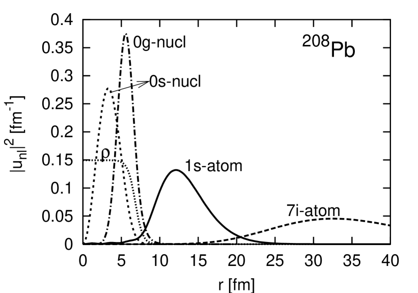
Figure 2: Top panel: Modulus squared of the $K^{-}-^{208}$Pb reduced radial wave functions for the 7i, the 1s atomic (Sect. 3) and the 0s and 0g nuclear (Sect. 4) levels as functions of $r$. Radial wave functions satisfy $\int_{0}^{\infty}dr~{}|u_{nl}(r)|^{2}=1$. We also show the nuclear density $\rho$ (fm^-3) in lead. Bottom panel: The product $\rho(r)\times|u_{nl}(r)|^{2}$ as a function of $r$. Here again the nuclear density, now in arbitrary units, is also plotted. All wave–functions have been obtained using $V_{\rm opt}^{\rm(1m)}$.

Figure 3: Same as in Fig.1.

To finish this section we would like to stress that the strong interaction effects in kaonic atoms are highly non-perturbative, as evidenced by the fact that although the level shifts are repulsive (i.e. negative) the real part of the optical potentials is attractive. This is a direct consequence of the absorptive part of the potentials being comparable in magnitude to the real part [6].

3 Deeply bound atomic $K^{-}$-nucleus levels

We have used the four previous $K^{-}$-nucleus optical potentials ($V_{\rm opt}^{\rm(1)}$, $V_{\rm opt}^{\rm(1m)}$, $V_{\rm opt}^{\rm(2)}$ and $V_{\rm opt}^{\rm(2DD)}$) to predict binding energies and widths of deeply bound atomic states, not yet observed, in ${}^{12}{\rm C}$, ${}^{40}{\rm Ca}$ and ${}^{208}{\rm Pb}$. Results for binding energies, strong shifts and widths are collected in Table 5. Binding energies, $B$, are practically independent of the used optical potential. Indeed, for a given nucleus and level, $B$ varies at most at the level of one per cent, hence we only present results obtained with the modified Oset-Ramos potential, $V_{\rm opt}^{\rm(1m)}$. Deeply bound atomic level widths are much more sensitive to the details of the potential, and approximately follow a regular pattern: $V_{\rm opt}^{\rm(2)}-$widths are the widest, those calculated with the $V_{\rm opt}^{\rm(2DD)}$ potential are narrower than the first ones by a few per cent, as it was previously stated in Ref. [24]. For the deepest states, the $V_{\rm opt}^{\rm(1m)}$ interaction leads to significantly smaller widths (about 20 to 40 %) than the $V_{\rm opt}^{\rm(2)}$ potential. On the other hand, $V_{\rm opt}^{\rm(1m)}$ and $V_{\rm opt}^{\rm(2DD)}$ predictions are more similar, but one still finds appreciable differences. The narrowest widths are obtained with the $V_{\rm opt}^{\rm(1)}$ potential.

Nucleus	Atomic Level	$B$ [MeV]	$\varepsilon$ [MeV]	$\Gamma$ [MeV]
	$nl$	(1m)	(1m)	(1)	(1m)	(2)	(2DD)
12C	1s	$-$0.274	$-$0.158	0.049	0.036	0.064	0.055
	2s	$-$0.087	$-$0.024	0.009	0.007	0.012	0.010
	3s	$-$0.042	$-$0.008	0.003	0.002	0.004	0.003
	2p	$-$0.113	$-$0.001	0.001	0.002	0.001	0.001
40Ca	1s	$-$1.48	$-$1.961	0.374	0.456	0.469	0.414
	2s	$-$0.62	$-$0.436	0.105	0.128	0.131	0.117
	3s	$-$0.34	$-$0.161	0.043	0.053	0.054	0.048
	2p	$-$1.09	$-$0.202	0.133	0.127	0.171	0.164
	3p	$-$0.50	$-$0.069	0.046	0.044	0.059	0.057
	4p	$-$0.29	$-$0.031	0.021	0.020	0.027	0.026
	5p	$-$0.19	$-$0.016	0.011	0.011	0.014	0.014
	3d	$-$0.58	$-$0.004	0.007	0.007	0.008	0.008
	4d	$-$0.32	$-$0.002	0.004	0.004	0.005	0.004
	5d	$-$0.21	$-$0.001	0.002	0.002	0.003	0.003
208Pb	1s	$-$7.20	$-$10.5	1.39	1.42	1.75	1.60
	2s	$-$4.19	$-$5.20	0.656	0.657	0.818	0.749
	3s	$-$2.79	$-$2.70	0.367	0.366	0.457	0.418
	4s	$-$2.00	$-$1.55	0.227	0.226	0.283	0.258
	2p	$-$6.75	$-$6.02	1.20	1.38	1.49	1.38
	3p	$-$3.96	$-$2.88	0.574	0.661	0.714	0.663
	4p	$-$2.65	$-$1.57	0.326	0.373	0.404	0.376
	5p	$-$1.91	$-$0.939	0.203	0.232	0.252	0.235
	3d	$-$5.87	$-$2.70	0.833	0.848	1.04	0.959
	4d	$-$3.56	$-$1.38	0.424	0.432	0.529	0.486
	5d	$-$2.44	$-$0.792	0.249	0.254	0.310	0.285
	4f	$-$4.68	$-$0.796	0.418	0.468	0.522	0.492
	5f	$-$2.99	$-$0.502	0.245	0.271	0.305	0.288
	6f	$-$2.11	$-$0.321	0.154	0.168	0.191	0.181
	5g	$-$3.46	$-$0.098	0.109	0.118	0.136	0.129
	6g	$-$2.38	$-$0.087	0.086	0.095	0.108	0.102
	7g	$-$1.75	$-$0.066	0.062	0.069	0.077	0.073
	6h	$-$2.47	$-$0.004	0.009	0.009	0.011	0.011
	7h	$-$1.81	$-$0.005	0.010	0.010	0.013	0.013
	8h	$-$1.39	$-$0.005	0.009	0.009	0.011	0.011

Table 5: Total binding energies $B$, strong shifts $\varepsilon$, and widths $\Gamma$ of different deeply bound kaonic atom levels. Results for shifts and bindings are only presented for the potential $V_{\rm opt}^{\rm(1m)}$, whereas for the widths we give the results obtained with the four optical potentials considered in this work: $V_{\rm opt}^{\rm(1)}$, $V_{\rm opt}^{\rm(1m)}$, $V_{\rm opt}^{\rm(2)}$ and $V_{\rm opt}^{\rm(2DD)}$.

In Refs. [1] and  [9], and supported by the results obtained from the empirical $V_{\rm opt}^{\rm(2)}$ and $V_{\rm opt}^{\rm(2DD)}$ potentials, a scenario where the deep atomic states are narrow enough to be separated in most cases, except for some overlap in heavy nuclei, was firstly presented. The above discussion and the results presented in Table 5 for the more theoretical founded potentials $V_{\rm opt}^{\rm(1)}$ and $V_{\rm opt}^{\rm(1m)}$ reinforce such a scenario. To illustrate this point, we present in Fig. 4 binding energies and widths, using the $V_{\rm opt}^{\rm(1m)}$ potential, for different atomic states in carbon and lead to show how separable the different levels are.

Figure 4: Binding energies $B$ of deeply bound atomic levels in ¹²C and ²⁰⁸Pb. The error bar stands for the full width $\Gamma$ of each level. They have been computed using the $V^{\rm(1m)}_{\rm opt}$ potential.

As we mentioned in the introduction, the overlap of the $K^{-}$-wave-function and the nucleus is bigger for these low-lying atomic states than for those accessible via the atomic cascade (see Fig. 5), and thus the precise determination of their binding energies and widths would provide valuable details of the antikaon-nucleus interaction at threshold. Thus, several nuclear reactions have been already suggested to detect them [19] and [24]. A rough comparison of the typical values in Fig. 5 and those in the bottom panel of Fig. 2 helps us to understand why the typical energy-shifts and widths are of the order of the MeV for deep atomic states while the magnitude of those for high-lying (measured) atomic states was the KeV. The minima of the 1s-atomic modulus squared wave function in Fig. 5 hint the existence of deeper bound states, as it was discussed in Ref. [9]. Those states will be the subject of the next section.

Figure 5: As bottom panel of Fig. 2, but now for the deeply bound 1s atomic level, not yet detected.

	$K^{-}$ nuclear states
Nucleus	Nuclear level	(1)		(1m)		(2)		(2DD)
	$Nl$	$B$	$\Gamma$	$B$	$\Gamma$	$B$	$\Gamma$	$B$	$\Gamma$
12C	0s	$-$8.64	92.1	$-$22.1	43.6	$-$12.2	183	$-$153	216
	0p							$-$78.8	159
	0d							$-$6.54	108
40Ca	0s	$-$30.6	105	$-$44.0	45.8	$-$39.6	213	$-$92.5	162
	0p	$-$9.71	91.6	$-$22.3	43.3	$-$14.0	182	$-$43.1	128
208Pb	0s	$-$54.1	107	$-$66.1	49.2	$-$65.8	196	$-$197	205
	1s	$-$32.3	97.6	$-$43.5	46.8	$-$41.4	177	$-$160	181
	2s	$-$1.94	80.7	$-$14.0	38.5	$-$7.19	149	$-$110	152
	3s							$-$55.4	123
	4s							$-$0.623	88.0
	0p	$-$45.3	104	$-$56.9	48.5	$-$56.1	189	$-$182	196
	1p	$-$18.9	91.0	$-$30.1	44.4	$-$26.3	165	$-$138	168
	2p							$-$84.3	139
	3p							$-$28.7	108
	0d	$-$35.2	99.7	$-$46.4	47.5	$-$44.9	181	$-$166	185
	1d	$-$4.56	83.4	$-$16.1	40.6	$-$10.2	153	$-$115	155
	2d							$-$58.5	126
	0f	$-$23.9	94.9	$-$34.8	46.1	$-$32.2	172	$-$147	174
	1f							$-$91.0	143
	2f							$-$33.2	113
	0g	$-$11.4	89.4	$-$22.2	44.3	$-$18.2	161	$-$127	162
	1g							$-$66.8	131
	2g							$-$8.33	98.6

Table 6: Nuclear $K^{-}$ binding energies ($B$) and widths ($\Gamma$) for different levels ($N,l$), nuclei and optical potentials ($V_{\rm opt}^{\rm(1)}$, $V_{\rm opt}^{\rm(1m)}$, $V_{\rm opt}^{\rm(2)}$ and $V_{\rm opt}^{\rm(2DD)}$). All units are in MeV. $N$ does not necessarily denote the number of nodes of the complex wave function, and just stands for energy ordering.

4 Nuclear $K^{-}$ and $\bar{K}^{0}$ states

All four optical potentials defined in the previous sections also have $K^{-}-$nucleus bound levels much deeper and wider than the deep atomic states presented in Table 5. We call these levels nuclear states, an enlightening discussion on their nature and differences to the atomic states can be found in Ref. [25]. Those states would not exist if the strong interaction were switched off. To obtain all the nuclear levels for a given optical potential and nucleus, we initially set to zero the imaginary part of the optical potential and switch it on gradually keeping track at any step of the bound levels. We study three different nuclei across the periodic table (carbon, calcium and lead). Results are shown in Table 6. As can be seen, energies and widths depend greatly on the details of the used potential, however, and because of the enormous widths predicted for all of them, there exist serious doubts not only on the ability to resolve different states but also on their proper existence.

For the case of the atomic states discussed in the previous sections, the net effect of the strong potential was repulsive (negative energy shifts), whereas for these nuclear bound states, the resulting effect of the strong potential is attractive, as can be seen in Table 7 where we present $\bar{K}^{0}-$nuclear states. Assuming isospin symmetry and neglecting isovector effects, we obtain those neutral antikaon bound states just by switching off the electromagnetic potential. Looking at both tables (6 and 7), we see that the electromagnetic interaction does not affect at all the widths ($\Gamma$) of the deepest states. It has some effects on the binding energies ($B$), and, in some cases, it is responsible for the existence of some levels for $K^{-}$ and not for the $\bar{K}^{0}$ case. In any case, we are certainly dealing with a highly non-perturbative (non-linear) scenario. For instance, for all nuclei and levels, the widths are more or less the same and only depend significantly on the potential. This behavior is due to the fact that these nuclear wave–functions are totally inside of the nucleus (see for instance 0s and 0g nuclear $K^{-}-^{208}$Pb levels in Fig. 2) where all the optical potentials are practically constant and much bigger than the electromagnetic one, as can be seen in Fig. 1. Thus, the electromagnetic dynamics does not play a crucial role, as it is explicitly shown in Fig. 6, where we compare $K^{-}-$ and $\bar{K}^{0}-$nucleus wave functions in ²⁰⁸Pb. As a matter of fact the width of any of those levels approximately verifies $\Gamma/2\simeq-~{}{\rm Im}(V_{\rm opt})$ at the center of the nucleus.

Figure 6: Modulus squared of the $K^{-}-$ (solid) and $\bar{K}^{0}-$ (dashed) ²⁰⁸Pb reduced radial wave functions for the 0s and 0f nuclear states as functions of $r$. Radial wave functions satisfy $\int_{0}^{\infty}dr~{}|u_{nl}(r)|^{2}=1$. We also show the nuclear density $\rho$ (fm^-3) in lead. Wave–functions have been obtained using $V_{\rm opt}^{\rm(1m)}$.

The theoretical potential of Ref. [10] supplemented by the phenomenological piece $\delta V^{\rm fit}$ in Eq. (3), leads both to the best description of the measured kaonic atom data and to the narrowest nuclear antikaon states. Indeed, $V_{\rm opt}^{\rm(1m)}-$widths are about four or five times smaller than the ones predicted by the empirical $V_{\rm opt}^{\rm(2DD)}$ and $V_{\rm opt}^{\rm(2)}$ potentials. Actually, in some cases the $V_{\rm opt}^{\rm(1m)}-$interaction predicts states such that $B+\Gamma/2$ is still negative and thus, they might be interpreted as well defined states.

	$\bar{K}^{0}$ nuclear states
Nucleus	Nuclear level	(1)		(1m)		(2)		(2DD)
	$Nl$	$B$	$\Gamma$	$B$	$\Gamma$	$B$	$\Gamma$	$B$	$\Gamma$
12C	0s	$-$4.76	91.6	$-$18.3	43.4	$-$8.08	182	$-$149	216
	0p							$-$74.9	159
	0d							$-$2.83	107
40Ca	0s	$-$21.3	105	$-$34.7	45.8	$-$29.9	212	$-$83.3	162
	0p			$-$13.8	43.0	$-$4.69	181	$-$34.2	127
208Pb	0s	$-$31.1	107	$-$43.1	49.2	$-$42.4	195	$-$173	205
	1s	$-$10.2	96.4	$-$21.7	46.4	$-$18.7	176	$-$137	180
	2s							$-$87.9	152
	3s							$-$33.5	122
	0p	$-$23.4	103	$-$35.1	48.5	$-$33.7	188	$-$160	195
	1p			$-$8.88	43.4	$-$4.07	164	$-$115	167
	2p							$-$62.3	138
	0d	$-$14.1	98.6	$-$25.5	47.3	$-$23.1	179	$-$143	184
	1d							$-$92.6	154
	2d							$-$36.9	125
	0f			$-$14.6	45.8	$-$10.9	170	$-$125	173
	1f							$-$69.2	142
	0g							$-$106	162
	1g							$-$45.5	130

Table 7: Same as in Table 6 for $\bar{K}^{0}-$nuclear states.

5 Conclusions

We have shown that the theoretical potential $V^{(1)}_{\rm opt}$, recently developed by Ramos and Oset [10] and based on a chiral model, gives an acceptable description of the observed kaonic atom states, through the whole periodic table ($\chi^{2}/dof=3.8$). Furthermore, it also gives quite reasonable predictions (when compared to results obtained from other phenomenological potentials fitted to available data) for the deep kaonic atom states, not yet observed. This is noticeable, because it has no free parameters. Of course, it can be improved by adding to it a small empirical piece which is fitted to the all available kaonic atom data. In this way, we have constructed $V_{\rm opt}^{\rm(1m)}$, and have used it to both quantify the “deficiencies” of the microscopical potential of Ramos and Oset and also to achieve more reliable predictions for the deeper (atomic and nuclear) bound states not yet detected. From the first kind of studies, we have concluded that at low densities, the combined effect of both real and imaginary parts of the theoretical potential leads to energy shifts more repulsive than the experimental ones. More quantitative results can be drawn from Eq. (8). Besides, deeply bound atomic state energies and widths obtained with $V_{\rm opt}^{\rm(1m)}$ confirm the existence of narrow and separable states, as pointed out in Ref. [9], and therefore subject to experimental observation by means of nuclear reactions. However, there exist appreciable differences among the predicted widths for these states, when different potentials are used. Thus, the detection of such states would shed light on the intricacies of the antikaon behavior inside of a nuclear medium.

Finally, we have calculated nuclear antikaon states, for which the electromagnetic dynamics does not play a crucial role. There, we are in highly non-perturbative regime and their widths depend dramatically on the used potential, but they do not depend on the nucleus or level. However, because of the huge values found for the widths, one might have some trouble in identifying them as states. In any case, $V_{\rm opt}^{\rm(1m)}$ leads to the narrowest states, and in some cases and using $l$-selective nuclear reactions one might resolve some states (for instance the ground state in ⁴⁰Ca, see Tables 6 and  7).

To end the paper, we would like to point out, that one should be cautious when interpreting results and conclusions drawn for the deep atomic and nuclear states, not yet detected. For instance, though it is commonly accepted that $p$-wave and isovector corrections to the optical potential have little effect at the low densities explored by the available data, it is not necessarily true at the higher densities explored by deeper bound states.

References

- [1] C.J.Batty, E. Friedman and A. Gal, Phys. Rep. 287 (1997) 385.
- [2] E. Friedman and G. Soff, Journal of Physics G11 (1985) L37.
- [3] H. Toki and T. Yamazaki, Phys. Lett. B213 (1988) 129.
- [4] J. Nieves, E. Oset and C. Garcia-Recio, Nucl. Phys. A554 (1993) 509.
- [5] T. Yamazaki, et. al.; Z. Phys. A335 (1996) 219.
- [6] E. Friedman, A. Gal and C.J. Batty, Nucl.Phys.A579 (1994) 518.
- [7] E. Friedman, A. Gal and C.J. Batty, Phys. Lett. B308 (1993) 6.
- [8] E. Friedman, A. Gal, J. Mares and A. Cieply, Phys.Rev. C60 (1999) 024314.
- [9] E. Friedman and A. Gal, Phys.Lett. B459 (1999) 43.
- [10] A. Ramos and E. Oset, Nucl. Phys. A in print, nucl-th/9906016 .
- [11] E. Oset and A. Ramos, Nucl. Phys. A635 (1998) 99.
- [12] N. Kaiser, P.B. Siegel and W. Weise, Nucl. Phys. A594 (1995) 325; ibidem Phys. Lett. B362 (1995) 23.
- [13] N. Kaiser, T. Waas and W. Weise, Nucl. Phys. A612 (1997) 297.
- [14] J.A. Oller and E. Oset, Nucl. Phys. A620 (1997) 438; J.A. Oller, E. Oset and J.R. Peláez, Phys. Rev. Lett. 80 (1998) 3452; ibidem, Phys. Rev. D59 (1991) 074001.
- [15] J. Nieves and E. Ruiz Arriola, Phys. Lett. B455 (1999) 30; ibidem, hep-ph/9907469.
- [16] M. F. M. Lutz, Phys.Lett. B426 (1998) 12-20; and preprint nucl-th/9802033.
- [17] J. Schaffner-Bielich, V. Koch and M. Effenberger, Nucl. Phys. A in print, nucl-th/9907095.
- [18] D.B. Kaplan and A. E. Nelson, Phys. Lett. B175 (1986) 57.
- [19] S. Hirenzaki, Y. Okumura, H. Toki, E. Oset and A. Ramos, Phys. Rev. C in print; ibidem, PANIC 99 Abstracts (Uppsala University, 1999), p. 201.
- [20] C. Itzykson and B. Zuber, Quantum Field Thoery, McGraw-Hill (1969) New York.
- [21] C.W. de Jager, H. de Vries and C. de Vries, At. Data and Nucl. Data Tables 14 (1974) 479; 36 (1987) 495.
- [22] J.W. Negele and D. Vautherin, Phys. Rev. C11 (1975) 1031 and references therein.
- [23] C. Garcia-Recio, L.L. Salcedo and E. Oset, Phys. Rev. C39 (1989) 595.
- [24] E. Friedman and A. Gal, Nucl. Phys. A658 (1999) 345.
- [25] A. Gal, E. Friedman and C.J. Batty, Nucl. Phys. A606 (1996) 283.