Cranked Relativistic Hartree-Bogoliubov Theory: Formalism and Application to the Superdeformed Bands in the $A\sim 190$ region

Abstract

Cranked Relativistic Hartree-Bogoliubov theory without and with approximate particle number projection by means of the Lipkin-Nogami method is presented in detail as an extension of Relativistic Mean Field theory with pairing correlations to the rotating frame. Pairing correlations are taken into account by a finite range two-body force of Gogny type. The applicability of this theory to the description of rotating nuclei is studied in detail on the example of superdeformed bands in even-even nuclei of the $A\sim 190$ mass region. Different aspects such as the importance of pairing and particle number projection, the dependence of the results on the parametrization of the RMF Lagrangian and Gogny force etc. are investigated in detail. It is shown that without any adjustment of new parameters the best description of experimental data is obtained by using the well established parameter sets NL1 for the Lagrangian and D1S for the pairing force. Contrary to previous studies at spin zero it is found that the increase of the strength of the Gogny force is not necessary in the framework of Relativistic Hartree-Bogoliubov theory provided that particle number projection is performed.

PACS numbers: 21.60.-n, 21.60.Cs, 21.60.Jx, 27.80.+w

Keywords: Cranked Relativistic Hartree-Bogoliubov theory, Gogny forces, particle number projection, superdeformation

I Introduction

The development of self-consistent microscopic many-body mean field theories aimed on the description of low-energy nuclear phenomena provides necessary theoretical tools for an exploration of the nuclear chart into know and unknown regions. This development is motivated by theoretical and experimental reasons. Compared with conventional approaches such as, for example, the macroscopic+microscopic method, self-consistent theories rely on a smaller number of assumptions and start from a more microscopic level. For example, the starting point of non-relativistic mean field theories is an effective interaction between nucleons constituting the nucleus. Such theories based either on zero range Skyrme forces or finite range Gogny forces have been widely used starting from seventies. The next step is replacing the Schrödinger equation by the Dirac equation and thus considering the relativistic mean field (RMF) theory [1]. In RMF theory, the nucleus is described as a system of point-like nucleons, Dirac spinors, which interact in a phenomenological way by the exchange of mesons, such as the $\sigma$-meson responsible for the large scalar attraction at intermediate distances, the $\omega$-meson for the vector repulsion at short distances and the $\rho$-meson for the asymmetry properties of nuclei with large neutron or proton excess. Such a description has a clear advantage that the spin-orbit splitting, which plays an extremely important role in low-energy nuclear physics, emerges in a natural way as a genuine relativistic effect. In addition, the pseudo-spin symmetry, the origin of which was a long-standing puzzle, does find a natural explanation in the framework of RMF theory [2]. RMF theory has been extremely successful also in the description of many other facets of low-energy nuclear physics, such as ground state properties, giant resonances, superdeformed rotating nuclei etc., see Ref. [3] for an overview.

Since the discovery of the first superdeformed rotational (SD) band in ¹⁵²Dy [4], the investigation of superdeformation at high angular momentum remains one of the most challenging topics of nuclear structure. The rich variety of physical phenomena at superdeformed shapes is based on a complicated and rather subtle interplay of collective and single-particle properties. Although at the present stage, a general understanding of this phenomenon has been achieved, there are still many unresolved questions related, for example, to the phenomenon of identical bands and to the treatment of pairing correlations. In addition, the microscopic theoretical models used so far are still far from a precise quantitative description of SD bands which indicates the necessity of further improvements. Different theoretical methods based mainly on the concept of the cranking model of Inglis [5] have been employed for the quantitative description of various high-spin phenomena at SD shapes, see for example recent overviews in Refs. [6, 7]. The cranked version of the RMF theory - the Cranked Relativistic Mean Field (CRMF) theory [8, 9, 10, 11] is amongst the most successful ones. It has been applied in a systematic way to the description of SD bands in different mass regions such as $A\sim 60$ [12, 13, 14, 15], $A\sim 80$ [16] and $A\sim 140-150$ [10, 11, 17, 18, 19]. Pairing correlations are expected to be considerably quenched in SD bands of these regions at high spin and thus they have been neglected in all studies quoted above. One should clearly recognize that the neglect of pairing correlations is an approximation because pairing correlations being weak are still present even at the highest rotational frequencies. Despite this a very successful description of many properties of SD bands, such as dynamic $J^{(2)}$ and kinematic $J^{(1)}$ moments of inertia, absolute and relative charge quadrupole moments, effective alignments $i_{eff}$, single-particle properties in the SD minimum etc., has been obtained in these studies in an unpaired formalism.

However, the rotational properties of nuclei at low and medium spin are strongly affected by pairing correlations. In order to describe such properties within the relativistic framework, we have developed the Cranked Relativistic Hartree-Bogoliubov (CRHB) theory. This theory is an extension of CRMF theory to the description of pairing correlations in rotating nuclei. The brief outline of this theory and its application to the study of several yrast SD bands observed in the $A\sim 190$ mass region has been reported in Ref. [20]. The present manuscript represents an extension of this investigation where both the theoretical formalism and the calculations will be presented in much greater details.

The paper is organized in the following way: In Section II a detailed description of the CRHB theory without and with approximate particle number projection by means of the Lipkin-Nogami method and some of the specific features of the present calculations are presented. The shell structure in the $A\sim 190$ mass region of superdeformation and the impact of pairing and particle number projection on the rotational and deformation properties of rotating nuclei are investigated in detail on the example of the lowest SD bands in ¹⁹²Hg and ¹⁹⁴Pb nuclei in Section III. In Section IV, we study the dependence of the results of CRHB calculations with particle number projection on the parametrization of the RMF Lagrangian and the Gogny force using SD bands in ¹⁹⁴Hg and ¹⁹⁴Pb as an example. The properties of yrast SD bands observed so far in even-even nuclei of the $A\sim 190$ mass region are systematically studied in Section V. Finally, Section VI summarizes our main conclusions.

II Cranked Relativistic Hartree-Bogoliubov (CRHB) Theory

A The CRHB equations

In relativistic mean field (RMF) theory the nucleus is described as a system of point-like nucleons, Dirac spinors, coupled to mesons and to the photons. The nucleons interact by the exchange of several mesons, namely a scalar meson $\sigma$ and three vector particles $\omega$, $\rho$ and the photon. The isoscalar-scalar $\sigma$-mesons provide a strong intermediate range attraction between the nucleons. For the three vector particles we have to distinguish the time-like components and the spatial components. For the photons this means the Coulomb field and possible magnetic field in the case where currents play a role. For the isoscalar-vector $\omega$-meson the time-like component provides a very strong repulsion at short distances for all combinations of particles, $pp$, $nn$ and $pn$. For the isovector-vector $\rho$-meson the time-like components give rise to a short range repulsion for like particles ($pp$ and $nn$) and a short range attraction for unlike particles ($np$). They also have a strong influence on the symmetry energy. In addition, the spatial components of the $\omega$ and $\rho$-mesons lead to an interaction between possible currents, which are for the $\omega$-meson attractive for all combinations ($pp$, $nn$ and $pn$-currents) and for the $\rho$-meson attractive for $pp$ and $nn$-currents but repulsive for $pn$-currents. We have to keep in mind, however, that within mean field theory these currents only occur in cases of time-reversal breaking mean fields as, for instance, in the case of the Coriolis fields.

The starting point of RMF theory is the well known local Lagrangian density

$${\cal L} = \bar{\psi}(i\gamma^{\mu}\partial_{\mu}-m)\psi+\frac{1}{2}(\partial_{\mu}\sigma\partial^{\mu}\sigma-m_{\sigma}^{2}\sigma^{2})-\frac{1}{3}g_{2}\sigma^{3}-\frac{1}{4}g_{3}\sigma^{4}$$ (3)

$$-\frac{1}{4}{\Omega}_{\mu\nu}{\Omega}^{\mu\nu}+\frac{1}{2}m_{\omega}^{2}\omega_{\mu}\omega^{\mu}~{}-~{}\frac{1}{4}{\vec{R}}_{\mu\nu}{\vec{R}}^{\mu\nu}+\frac{1}{2}m_{\rho}^{2}\vec{\rho}_{\mu}\vec{\rho\,}^{\mu}~{}-~{}\frac{1}{4}F_{\mu\nu}F^{\mu\nu}$$

$$-g_{\sigma}\bar{\psi}\sigma\psi~{}-~{}g_{\omega}\bar{\psi}\gamma^{\mu}\omega_{\mu}\psi~{}-~{}g_{\rho}\bar{\psi}\gamma^{\mu}\vec{\tau}\vec{\rho}_{\mu}\psi~{}-~{}e\,\bar{\psi}\gamma^{\mu}\,\frac{1-\tau_{3}}{2}A_{\mu}\psi,$$

where the non-linear self-coupling of the $\sigma$-field, which is important for an adequate description of nuclear surface properties and the deformations of finite nuclei, is taken into account according to Ref. [21]. The Lagrangian (3) contains as parameters the masses of the mesons $m_{\sigma}$, $m_{\omega}$ and $m_{\rho}$, the coupling constants $g_{\sigma}$, $g_{\omega}$ and $g_{\rho}$ and the non-linear terms $g_{2}$ and $g_{3}$. The field tensors for the vector mesons and the photon field are:

$${\Omega}_{\mu\nu}=\partial_{\mu}\omega_{\nu}-\partial_{\nu}\omega_{\mu},\qquad{\vec{R}}_{\mu\nu}=\partial_{\mu}\vec{\rho}_{\nu}-\partial_{\nu}\vec{\rho}_{\mu},\qquad F_{\mu\nu}=\partial_{\mu}A_{\nu}-\partial_{\nu}A_{\mu}.$$ (4)

In the present state of the art of the RMF theory, the meson and photon fields are treated as classical fields.

Two approximations, namely the mean-field approximation, in which the meson field operators are replaced by their expectation values

$$\langle\sigma\rangle=\sigma_{0},\,\,\,\,\,\,\,\langle\omega_{\mu}\rangle=\delta_{\mu 0}\omega_{0}$$ (5)

which is justified by the fact that the source terms are large [1], and the No-sea approximation, in which only positive-energy states are taken into account [22], are employed in order to solve the Lagrangian (3).

For classical fields we can restrict ourselves to the intrinsic symmetry violating product wave function $|\Phi\rangle$ which can be represented as a generalized Slater determinant. As long as we consider time-independent static or quasistatic fields, this limits the applicability of CRHB theory to the yrast bands and to the excited bands of dominantly quasiparticle nature. In particular, the bands based on low-lying collective vibrations, such as for example $\gamma$-, $\beta$-vibrational bands, cannot be described in the present formalism since they have (for example, in even-even nuclei) an intrinsic wave function which is a linear superposition of many two-quasiparticle states. In order to study such bands one should employ time-dependent fields in the random phase approximation in the rotating frame: the task which has so far been resolved only in simple non-relativistic models with separable forces [23].

As discussed in detail in Refs. [8, 24, 25] in the unpaired formalism, the transformation to the rotating frame within the framework of the cranking model leads to the cranked relativistic mean field equations. Note that in the present investigation we restrict ourselves to one-dimensional rotation with rotational frequency $\Omega_{x}$ around the $x$-axis. Since pairing correlations work only between the fermions, the Bogoliubov transformation affects directly only the fermionic part. Thus the time-independent inhomogeneous Klein-Gordon equations for the mesonic fields obtained by means of variational principle are given in the CRHB theory by [20]

$$\left\{-\Delta-({\Omega}_{x}\hat{L}_{x})^{2}+m_{\sigma}^{2}\right\}~{}\sigma({\mbox{\boldmath$r$}}) = -g_{\sigma}\rho_{\sl s}({\mbox{\boldmath$r$}})$$ (6)

$$\,\,\,\,\,\,\,\,\,\,\,\,\,\,\,\,\,-g_{2}\sigma^{2}({\mbox{\boldmath$r$}})-g_{3}\sigma^{3}({\mbox{\boldmath$r$}}),$$ (7)

$$\left\{-\Delta-({\Omega}_{x}\hat{L}_{x})^{2}+m_{\omega}^{2}\right\}\omega_{0}({\mbox{\boldmath$r$}}) = g_{\omega}\rho_{\sl v}^{\it i\sl s}({\mbox{\boldmath$r$}}),$$ (8)

$$\left\{-\Delta-[{\Omega}_{x}(\hat{L}_{x}+\hat{S}_{x})]^{2}+m_{\omega}^{2}\right\}~{}{\mbox{\boldmath$\omega$}}({\mbox{\boldmath$r$}}) = g_{\omega}{\mbox{\boldmath$j$}}^{\it i\sl s}({\mbox{\boldmath$r$}}),$$ (9)

$$\left\{-\Delta-({\Omega}_{x}\hat{L}_{x})^{2}+m_{\rho}^{2}\right\}\rho_{0}({\mbox{\boldmath$r$}}) = g_{\rho}\rho_{\sl v}^{\it i\sl v}({\mbox{\boldmath$r$}}),$$ (10)

$$\left\{-\Delta-[{\Omega}_{x}(\hat{L}_{x}+\hat{S}_{x})]^{2}+m_{\rho}^{2}\right\}~{}{\mbox{\boldmath$\rho$}}({\mbox{\boldmath$r$}}) = g_{\rho}{\mbox{\boldmath$j$}}^{\it i\sl v}({\mbox{\boldmath$r$}}),$$ (11)

$$-\Delta~{}A_{0}({\mbox{\boldmath$r$}}) = e\rho_{\sl v}^{p}({\mbox{\boldmath$r$}}),$$ (12)

$$-\Delta~{}{\mbox{\boldmath$A$}}({\mbox{\boldmath$r$}}) = e{\mbox{\boldmath$j$}}^{p}({\mbox{\boldmath$r$}}),$$ (13)

where the source terms are sums of bilinear products of baryon amplitudes

$$\rho_{\sl s}({\mbox{\boldmath$r$}}) = \sum_{k>0}[V_{k}^{n}({\mbox{\boldmath$r$}})]^{\dagger}\hat{\beta}V_{k}^{n}({\mbox{\boldmath$r$}})+[V_{k}^{p}({\mbox{\boldmath$r$}})]^{\dagger}\hat{\beta}V_{k}^{p}({\mbox{\boldmath$r$}}),$$ (14)

$$\rho_{\sl v}^{\it i\sl s}({\mbox{\boldmath$r$}}) = \sum_{k>0}[V_{k}^{n}({\mbox{\boldmath$r$}})]^{\dagger}V_{k}^{n}({\mbox{\boldmath$r$}})+[V_{k}^{p}({\mbox{\boldmath$r$}})]^{\dagger}V_{k}^{p}({\mbox{\boldmath$r$}}),$$ (15)

$$\rho_{\sl v}^{\it i\sl v}({\mbox{\boldmath$r$}}) = \sum_{k>0}[V_{k}^{n}({\mbox{\boldmath$r$}})]^{\dagger}V_{k}^{n}({\mbox{\boldmath$r$}})-[V_{k}^{p}({\mbox{\boldmath$r$}})]^{\dagger}V_{k}^{p}({\mbox{\boldmath$r$}}),$$ (16)

$${\mbox{\boldmath$j$}}^{\it i\sl s}({\mbox{\boldmath$r$}}) = \sum_{k>0}[V_{k}^{n}({\mbox{\boldmath$r$}})]^{\dagger}\hat{{\mbox{\boldmath$\alpha$}}}V_{k}^{n}({\mbox{\boldmath$r$}})+[V_{k}^{p}({\mbox{\boldmath$r$}})]^{\dagger}\hat{{\mbox{\boldmath$\alpha$}}}V_{k}^{p}({\mbox{\boldmath$r$}}),$$ (17)

$${\mbox{\boldmath$j$}}^{\it i\sl v}({\mbox{\boldmath$r$}}) = \sum_{k>0}[V_{k}^{n}({\mbox{\boldmath$r$}})]^{\dagger}\hat{{\mbox{\boldmath$\alpha$}}}V_{k}^{n}({\mbox{\boldmath$r$}})-[V_{k}^{p}({\mbox{\boldmath$r$}})]^{\dagger}\hat{{\mbox{\boldmath$\alpha$}}}V_{k}^{p}({\mbox{\boldmath$r$}}).$$ (18)

The sums over $k>0$ run over all quasiparticle states corresponding to positive energy single-particle states (no-sea approximation). In Eqs. (13,18), the indexes $n$ and $p$ indicate neutron and proton states, respectively, and the indexes $\it i\sl s$ and $\it i\sl v$ are used for isoscalar and isovector quantities. $\rho_{\sl v}^{p}({\mbox{\boldmath$r$}})$, ${\mbox{\boldmath$j$}}^{p}({\mbox{\boldmath$r$}})$ in Eq. (13) correspond to $\rho_{\sl v}^{\it i\sl s}({\mbox{\boldmath$r$}})$ and ${\mbox{\boldmath$j$}}^{\it i\sl s}({\mbox{\boldmath$r$}})$ defined in Eq. (18), respectively, but with the sums over neutron states neglected. Note that the Coriolis term for the Coulomb potential $A_{0}({{\mbox{\boldmath$r$}}})$ and the spatial components of the vector potential ${\mbox{\boldmath$A$}}({\mbox{\boldmath$r$}})$ are neglected in Eqs. (13) since the coupling constant of the electromagnetic interaction is small compared with the coupling constants of the meson fields. On this classical level only the direct terms of the potentials are taken into account since most parametrizations of the RMF Lagrangian have been fitted to experimental data neglecting exchange terms. This means that the exchange terms are not fully neglected, but taken into account in an averaged way by adjusting the parameters of the direct terms.

The comparison of Eqs. (13,18) with Eqs. (4) and (5) in Ref. [11] indicates that the pairing correlations between the fermions have also an impact on mesonic fields through the redefinition of the various nucleonic densities and currents. While the occupation probabilities of the single-nucleon orbitals are equal 1 and 0 for the orbitals below and above the Fermi level in the systems with no pairing, they are between 0 and 1 when the pairing between the fermions is taken into account.

Contrary to the applications of the Hartree-(Fock)-Bogoliubov theory for the ground states of even-even nuclei, the time-reversal symmetry of the intrinsic wave function $|\Phi\rangle$ is broken by the Coriolis operator $\Omega_{x}\hat{J}_{x}$ ($\hat{J_{x}}$ is the projection of total angular momentum on the rotation axis) in the case of rotating nuclei. Therefore, we do not know a priori the conjugate states in the canonical basis and thus one must solve the full Hartree-Bogoliubov problem in the rotating frame [26, 27, 28]. The solution of this problem in the RMF theory is to large extent similar to the one obtained earlier in the non-relativistic case as far as we treat pairing in non-relativistic fashion as it is done in the CRHB theory. Thus in the following discussion we will mainly concentrate on the features specific for relativistic case.

The CRHB equations for the fermions in the rotating frame are given in one-dimensional cranking approximation by

$$\pmatrix{\hat{h}_{D}-\lambda_{\tau}-\Omega_{x}\hat{J}_{x}&\hat{\Delta}\cr-\!\hat{\Delta}^{*}&-\hat{h}^{*}_{D}+\lambda_{\tau}+\Omega_{x}\hat{J}^{*}_{x}\cr}\pmatrix{U_{k}({\mbox{\boldmath$r$}})\cr V_{k}({\mbox{\boldmath$r$}})}=E_{k}\pmatrix{U_{k}({\mbox{\boldmath$r$}})\cr V_{k}({\mbox{\boldmath$r$}})}$$ (19)

where $\hat{h}_{D}$ is the Dirac Hamiltonian for the nucleon with mass $m$

$$\hat{h}_{D}={\mbox{\boldmath$\alpha$}}(-i{\mbox{\boldmath$\nabla$}}-{\mbox{\boldmath$V$}}({\mbox{\boldmath$r$}}))~{}+~{}V_{0}({\mbox{\boldmath$r$}})~{}+~{}\beta(m+S({\mbox{\boldmath$r$}}))$$ (20)

and $\lambda_{\tau}$ are the chemical potentials defined from the average particle number constraints for protons and neutrons ($\tau=p,n$)

$$\langle{\Phi}_{\Omega_{x}}|\hat{N}_{p}|{\Phi}_{\Omega_{x}}\rangle=Z,\qquad\langle{\Phi}_{\Omega_{x}}|\hat{N}_{n}|{\Phi}_{\Omega_{x}}\rangle=N.$$ (21)

The particle number expectation values $\langle{\Phi}_{\Omega_{x}}|\hat{N}_{\tau}|{\Phi}_{\Omega_{x}}\rangle$ are defined via the (normal) density matrices $\rho_{p}$ and $\rho_{n}$

$$\langle{\Phi}_{\Omega_{x}}|\hat{N}_{\tau}|{\Phi}_{\Omega_{x}}\rangle=Tr(\rho_{\tau})\qquad{\rm where}\qquad\rho_{\tau}=V^{*}_{\tau}V^{T}_{\tau}.$$ (22)

The Dirac Hamiltonian contains an attractive scalar potential $S({\mbox{\boldmath$r$}})$

$$S({\mbox{\boldmath$r$}})=g_{\sigma}\sigma({\mbox{\boldmath$r$}}),$$ (23)

a repulsive vector potential $V_{0}({\mbox{\boldmath$r$}})$

$$V_{0}({\mbox{\boldmath$r$}})~{}=~{}g_{\omega}\omega_{0}({\mbox{\boldmath$r$}})+g_{\rho}\tau_{3}\rho_{0}({\mbox{\boldmath$r$}})+e\frac{1-\tau_{3}}{2}A_{0}({\mbox{\boldmath$r$}}),$$ (24)

a magnetic potential ${\mbox{\boldmath$V$}}({\mbox{\boldmath$r$}})$

$${\mbox{\boldmath$V$}}({\mbox{\boldmath$r$}})~{}=~{}g_{\omega}{\mbox{\boldmath$\omega$}}({\mbox{\boldmath$r$}})+g_{\rho}\tau_{3}{\mbox{\boldmath$\rho$}}({\mbox{\boldmath$r$}})+e\frac{1-\tau_{3}}{2}{\mbox{\boldmath$A$}}({\mbox{\boldmath$r$}}),$$ (25)

and a Coriolis term

$$-{\Omega}_{x}\hat{J}_{x}~{}=~{}-{\Omega}_{x}(\hat{L}_{x}+\frac{1}{2}\hat{\Sigma}_{x}).$$ (26)

The latter two terms are the contributions to the mean field which break time-reversal symmetry and induce currents. In the Dirac equation the field ${\mbox{\boldmath$V$}}({\mbox{\boldmath$r$}})$ has the structure of a magnetic field. Time-reversal symmetry is broken when the orbitals which are time-reversal counterparts are not occupied pairwise. At no rotation, this usually takes place in one-(multi-)quasiparticle configurations where the magnetic potential $V$($r$) breaks time-reversal symmetry. In rotating nuclei the time-reversal symmetry is additionally broken by the Coriolis field. The nuclear currents of Eq. (13) are the sources for the space-like components of the vector ${\mbox{\boldmath$\omega$}}({\mbox{\boldmath$r$}})$, ${\mbox{\boldmath$\rho$}}({\mbox{\boldmath$r$}})$ and ${\mbox{\boldmath$A$}}({\mbox{\boldmath$r$}})$ fields which give rise to polarization effects in the Dirac spinors through the magnetic potential ${\mbox{\boldmath$V$}}({\mbox{\boldmath$r$}})$ of Eq. (25). This effect is commonly referred to as nuclear magnetism [8]. It turns out that it is very important to take it into account for the proper description of currents, magnetic moments [29] and moments of inertia [10]. In the present calculations the spatial components of the vector mesons are properly taken into account in a fully self-consistent way.

In Eq. (19), the rotational frequency $\Omega_{x}$ along the $x$-axis is defined from the condition [5]

$$J=\langle{\Phi}_{\Omega_{x}}\mid\hat{J}_{x}\mid{\Phi}_{\Omega_{x}}\rangle~{}=~{}\sqrt{I(I+1)}.$$ (27)

where $I$ is total nuclear spin. $U_{k}({\mbox{\boldmath$r$}})$ and $V_{k}({\mbox{\boldmath$r$}})$ are quasiparticle Dirac spinors and $E_{k}$ denotes the quasiparticle energies.

The pairing potential (field) $\hat{\Delta}$ in Eq. (19) is given by

$$\hat{\Delta}\equiv\Delta_{ab}~{}=~{}\frac{1}{2}\sum_{cd}V^{pp}_{abcd}\kappa_{cd}$$ (28)

where the indices $a,b,\dots$ denote quantum numbers which specify the single-particle states with the space coordinates $r$ as well as the Dirac and isospin indices $s$ and $\tau$. It contains the pairing tensor $\kappa$

$$\kappa=V^{*}U^{T}$$ (29)

and the matrix elements $V^{pp}_{abcd}$ of the effective interaction in the $pp$-channel.

The matrix elements $V_{abcd}^{pp}$ in the pairing channel can, in principle, be derived as a one-meson exchange interaction by eliminating the mesonic degrees of freedom in the model Lagrangian as discussed in detail in the relativistic Hartree-Bogoliubov model developed in Ref. [30]. However, the resulting pairing matrix elements obtained with the standard sets of the RMF theory are unrealistically large. In nuclear matter the strong repulsion produced by the exchange of vector mesons at short distances results in a pairing gap at the Fermi surface that is by factor of 3 too large. In addition, standard RMF parameters do not reproduce scattering data in the $S_{0}$-channel, which is necessary for a reasonable description of pairing correlations. On the other hand, since we are using effective forces, there is no fundamental reason to have the same interaction both in the particle-hole and particle-particle channel [28]. In a first-order approximation, the effective interaction contained in the mean field $\hat{\Gamma}$ is a $G$ matrix, i.e. the sum over all ladder diagrams. On the contrary, the effective force in the $pp$ channel (pairing potential $\hat{\Delta}$) should be the $K$ matrix, the sum of all diagrams irreducible in $pp$ direction. Although encouraging results have been reported in applications to nuclear matter [31, 32], a microscopic and fully relativistic derivation of the pairing force starting from the Lagrangian of quantum hadrodynamics still cannot be applied to realistic nuclei. Thus we follow the prescription of Ref. [33] and use a phenomenological interaction of Gogny type with finite range (see Eq. (30) below) in the particle-particle channel. Such a procedure provides both the automatic cutoff of high-momentum components and, as follows from non-relativistic and relativistic studies, a reliable description of pairing properties in finite nuclei.

Although this procedure formally breaks the Lorentz structure of the RMF equations, one has to keep in mind that pairing itself is a completely non-relativistic phenomenon. Relativistic effects such as the nuclear saturation mechanism due to the cancellation between attractive scalar and repulsive vector potentials, spin-orbit splitting and the admixture of small components through the kinetic term $-i{\mbox{\boldmath$\alpha$}}{\mbox{\boldmath$\nabla$}}$ of the Dirac equation [3] are only important for the mean field part of Hartree-Bogoliubov theory and have only a negligible counterpart in the pairing field. The pairing density $\kappa$ and the corresponding pairing field result from the scattering of pairs in the vicinity of the Fermi surface. The pairing density is concentrated in an energy window of a few MeV around the Fermi level, i.e. the contributions from the small components of the wave functions to the pairing tensor $\kappa$ are very small. Thus in the present version of the CRHB theory, pairing correlations are only considered between the positive energy states. Consequently, it is justified to approximate the pairing force by the best currently available non-relativistic interaction: the pairing part of the Gogny force. At present, this is certainly more realistic than the use of a one-meson exchange force in the pairing channel, since this type of interactions has never been optimized for the description of pairing properties in finite nuclei. Thus the word relativistic in CRHB applies only to the Hartree particle-hole channel of this theory.

The phenomenological Gogny-type finite range interaction is given by

$$V^{pp}(1,2)=f\sum_{i=1,2}e^{-[({{\mbox{\boldmath$r$}}}_{1}-{{\mbox{\boldmath$r$}}}_{2})/\mu_{i}]^{2}}\times(W_{i}+B_{i}P^{\sigma}-H_{i}P^{\tau}-M_{i}P^{\sigma}P^{\tau})$$ (30)

where $\mu_{i}$, $W_{i}$, $B_{i}$, $H_{i}$ and $M_{i}$ $(i=1,2)$ are the parameters of the force and $P^{\sigma}$ and $P^{\tau}$ are the exchange operators for the spin and isospin variables, respectively. This interaction is density-independent. In most of the applications of the CRHB theory in the present article, the parameter set D1S [34] (see also Table I) is employed for the Gogny force. Note also that an additional factor $f$ affecting the strength of the Gogny force is introduced in Eq. (30). This is motivated by the fact that previous studies of different nuclear phenomena within the Relativistic Hartree-Bogoliubov theory followed the prescription of Ref. [33] where $f=1.15$ was employed. It turns out, however, that the rotational properties of the SD bands are very well described with $f=1.0$ if the approximate particle number projection is performed by means of the Lipkin-Nogami method. Thus the value $f=1.0$ is used in the following if no other value is specified.

In Hartree-(Fock)-Bogoliubov calculations the size of the pairing correlations is usually measured in terms of the pairing energy defined as

$$E_{pairing}~{}=~{}-\frac{1}{2}\mbox{Tr}(\Delta\kappa).$$ (31)

This is not an experimentally accessible quantity, but it is a measure for the size of the pairing correlations in the theoretical calculations. An alternative way to look for the size of pairing correlations is to use the BCS-like pairing energies defined as a difference between the total energies obtained at a given spin $I$ in the calculations with ($E_{\rm CRHB}(I)$) and without ($E_{\rm CRMF}(I)$) pairing

$$E_{\rm BCS}(I)=E_{\rm CRHB}(I)-E_{\rm CRMF}(I)$$ (32)

The quantities $E_{\rm BCS}$ and $E_{pairing}$ coincide only in the BCS approximation. The disadvantage of the use of the BCS-like pairing energies is related to the fact that the calculations with and without pairing should be performed in order to define this quantity in a proper way.

The total energy of system in the laboratory frame is given by

$$E_{\rm CRHB}=E^{\rm F}+E^{\rm B}$$ (33)

where $E^{\rm F}$ and $E^{\rm B}$ are the contributions from fermionic and mesonic (bosonic) degrees of freedom. Fermionic energies $E^{\rm F}$ are given by

$$E^{\rm F}=E_{part}+\Omega_{x}J+E_{pairing}+E_{cm}$$ (34)

where

$$E_{part}=Tr(h_{D}\rho),\qquad\qquad J=Tr(j_{x}\rho),$$ (35)

are the particle energy and the expectation value of the total angular momentum along the rotational axis and

$$E_{cm}=-\frac{3}{4}\hbar\omega_{0}=-\frac{3}{4}41A^{-1/3}\,\,\,\,{\rm MeV}$$ (36)

is the correction for the spurious center-of-mass motion approximated by its value in a non-relativistic harmonic oscillator potential.

The bosonic energies $E^{\rm B}$ in the laboratory frame are given by

$$E^{\rm B}= -~{}\frac{1}{2}\int d{{\mbox{\boldmath$r$}}}\,[g_{\sigma}\,\sigma({\mbox{\boldmath$r$}})\rho_{\sl s}({\mbox{\boldmath$r$}})+\frac{1}{3}g_{2}\sigma^{3}({\mbox{\boldmath$r$}})+\frac{1}{2}g_{3}\sigma^{4}({\mbox{\boldmath$r$}})]$$ (42)

$$-~{}\frac{1}{2}\,g_{\omega}\int d{{\mbox{\boldmath$r$}}}\,[\omega_{0}({\mbox{\boldmath$r$}})\rho_{\sl v}^{\it i\sl s}({\mbox{\boldmath$r$}})-{\mbox{\boldmath$\omega$}}({\mbox{\boldmath$r$}}){\mbox{\boldmath$j$}}^{\it i\sl s}({\mbox{\boldmath$r$}})]$$

$$-~{}\frac{1}{2}\,g_{\rho}\int d{{\mbox{\boldmath$r$}}}\,[\rho_{0}({\mbox{\boldmath$r$}})\rho_{\sl v}^{\it i\sl v}({\mbox{\boldmath$r$}})-{\mbox{\boldmath$\rho$}}({\mbox{\boldmath$r$}}){\mbox{\boldmath$j$}}^{\it i\sl v}({\mbox{\boldmath$r$}})]$$

$$-~{}\frac{1}{2}\,e\int d{{\mbox{\boldmath$r$}}}\left[A_{0}({\mbox{\boldmath$r$}})\rho_{\sl v}^{p}({\mbox{\boldmath$r$}})+{\mbox{\boldmath$A$}}({\mbox{\boldmath$r$}}){\mbox{\boldmath$j$}}^{p}({\mbox{\boldmath$r$}})\right]$$

$$+~{}{\Omega}_{x}^{2}\int d{{\mbox{\boldmath$r$}}}\,[\sigma({\mbox{\boldmath$r$}})\hat{L}_{x}^{2}\sigma({\mbox{\boldmath$r$}})-\omega_{0}({\mbox{\boldmath$r$}})\hat{L}_{x}^{2}\omega_{0}({\mbox{\boldmath$r$}})+{\mbox{\boldmath$\omega$}}({\mbox{\boldmath$r$}})(\hat{L}_{x}+\hat{S}_{x})^{2}{\mbox{\boldmath$\omega$}}({\mbox{\boldmath$r$}})$$

$$\qquad\qquad\qquad-\rho_{0}({\mbox{\boldmath$r$}})\hat{L}_{x}^{2}\rho_{0}({\mbox{\boldmath$r$}})+{\mbox{\boldmath$\rho$}}({\mbox{\boldmath$r$}})(\hat{L}_{x}+\hat{S}_{x})^{2}{\mbox{\boldmath$\rho$}}({\mbox{\boldmath$r$}})]$$

In the systems with broken time-reversal symmetry the spatial components of the $\omega$-mesons give larger contributions to the total energy than the ones of the $\rho$-mesons because of the isovector nature of the $\rho$-meson. One should also note that the contribution of the terms proportional to ${\Omega}_{x}^{2}$ to the total energy is very small being typically in the range of $\sim 10-20$ keV at the highest frequencies of interest in the $A\sim 190$ mass region and thus, in general, can be neglected.

B The Lipkin-Nogami Method

In recent years it has become clear that a proper treatment of pairing correlations is required to describe many nuclear properties. One should note that the Bogoliubov transformation is not commutable with the nucleon number operator and consequently the resulting wave function does not correspond to a system having a definite number of protons and neutrons. The best way to deal with this problem would be to perform an exact particle number projection before the variation [28]. However, for heavy nuclei this has been realized so far only for non-relativistic separable models [36] in part due to the fact that such calculations are expected to be extremely time-consuming for realistic interactions. As a result, an approximate particle number projection by means of the Lipkin-Nogami (LN) method [37, 38, 39, 40] (further APNP(LN)) is most widely used just because of its simplicity. As illustrated by the results of non-relativistic [41, 42, 43, 44, 45, 35, 46, 47] and recent relativistic [20, 48] calculations, the application of this method considerably improves an agreement with experiment especially for rotational properties of nuclei compared with the calculations without particle number projection.

Our derivation of the Lipkin-Nogami method is based on the Kamlah expansion [49] which is an approximation to the exact projection methods. It is applied to the two-body interaction $V^{pp}$ in the pairing channel. Note that the Gogny force in the pairing channel is density independent in the CRHB theory. For the derivation of the Lipkin-Nogami method with density dependent forces see Refs. [44, 35].

In the following discussion, we will limit ourselves to one type of particles. In the numerical calculations we use this approach for protons and neutrons separately. The eigenstates $|\Psi^{N}\rangle$ of the particle number operator $\hat{N}$ can be constructed from particle number violating Bogoliubov wave functions $|\Phi\rangle$ by means of the particle number projection operator $\hat{P}^{N}$

$$|\Psi^{N}\rangle=\hat{P}^{N}|\Phi\rangle=\frac{1}{2\pi}\int_{0}^{2\pi}\,d\phi e^{i(\hat{N}-N)\phi}|\Phi\rangle$$ (43)

where $N$ is actual particle number. With this wave function one obtains the total particle number projected energy

$$E^{N}_{proj}=\frac{\langle\Phi|\hat{H}\hat{P}^{N}|\Phi\rangle}{\langle\Phi|\hat{P}^{N}|\Phi\rangle}=\frac{\int_{0}^{2\pi}\,d\phi e^{-i\phi N}h(\phi)}{\int_{0}^{2\pi}\,d\phi e^{-i\phi N}n(\phi)}.$$ (44)

In the case of large particle number and strong deformations in gauge space one expects that the Hamiltonian and norm overlap integrals

$$h(\phi)=\langle\Phi|\hat{H}e^{i\phi\hat{N}}|\Phi\rangle\mbox{~{}~{}~{}~{}and~{}~{}}n(\phi)=\langle\Phi|e^{i\phi\hat{N}}|\Phi\rangle,$$ (45)

are sharply peaked at $\phi=0$ and are very small elsewhere. In addition, the quotient $h(\phi)/n(\phi)$ should be a rather smooth function. In such a case one can make an expansion of $h(\phi)$ in terms of $n(\phi)$ in the following way

$$h(\phi)=\sum_{m=0}^{M}\lambda_{m}\hat{\cal{N}}^{m}n(\phi)$$ (46)

where the Kamlah operator

$$\hat{\cal{N}}=\frac{1}{i}\frac{\partial}{\partial\phi}-\langle\Phi|\hat{N}|\Phi\rangle$$ (47)

represents the particle number operator in the space of the gauge angle $\phi$ and $\lambda_{m}$ are constants. Mathematically, Eq. (46) essentially corresponds to a Taylor expansion of the Fourier transformed function $h(\phi)/n(\phi)$ [28]. $M$ in Eq. (46) represents the order of expansion, for $M\rightarrow\infty$ this equation is exact. Since we need $h(\phi)$ only in the vicinity of $\phi=0$ we can already hope to get a very good approximation for this function with a few non-vanishing constants $\lambda_{0},\lambda_{1},\lambda_{2},...$, if they are properly adjusted. The number $M$ certainly depends on the widths of the overlap integral $n(\phi)$ which reflects the symmetry violation. The larger the symmetry violation, the better the approximation will already be for low $M$-values.

Inserting Kamlah operator into Eq. (46) one gets

$$h(\phi)=\sum_{m=0}^{M}\lambda_{m}\langle\Phi|(\Delta\hat{N})^{m}e^{i\phi\hat{N}}|\Phi\rangle\mbox{~{}~{}~{}~{}with ~{}~{}~{}~{}~{}}\Delta\hat{N}=\hat{N}-\langle\Phi|\hat{N}|\Phi\rangle.$$ (48)

The expansion coefficients $\lambda_{m}$ are determined by applying the operators $\hat{\cal N}^{k}$ $(k=0,1,...M)$ on Eq. (46)

$$\hat{\cal{N}}^{k}h(\phi)=\sum_{m=0}^{M}\lambda_{m}\hat{\cal{N}}^{m+k}n(\phi)\,\,,\mbox{~{}~{}~{}~{}~{}}k=0\ldots M\,.$$ (49)

This yields

$$\langle\Phi|(\Delta\hat{N})^{k}\hat{H}e^{i\phi\hat{N}}|\Phi\rangle=\sum_{m=0}^{M}\lambda_{m}\langle\Phi|(\Delta\hat{N})^{m+k}e^{i\phi\hat{N}}|\Phi\rangle\,.$$ (50)

Taking the limit $\phi\rightarrow 0$ this results in a system of the $M+1$ linear equations

$$\langle\Phi|[\hat{H}-\sum_{m=0}^{M}\lambda_{m}(\Delta\hat{N})^{m}](\Delta\hat{N})^{k}|\Phi\rangle=0$$ (51)

for the constants $\lambda_{m}$. The case of $M=1$ corresponds to CRHB theory discussed in Sect. II A. In the following we will use the shorthand notation $\langle\hat{O}\rangle=\langle\Phi|\hat{O}|\Phi\rangle$. In the case of $M=2$, the solution of the system of Eqs. (51) under the particle number constraint $\langle\Delta\hat{N}\rangle=0$ leads to the following values of $\lambda_{0},\lambda_{1},\lambda_{2}$:

$$\lambda_{0} = \langle\hat{H}\rangle-\lambda_{2}\langle(\Delta\hat{N})^{2}\rangle\,,$$ (52)

$$\lambda_{1} = \frac{\langle\hat{H}\Delta\hat{N}\rangle-\lambda_{2}\langle(\Delta\hat{N})^{3}\rangle}{\langle(\Delta\hat{N})^{2}\rangle}\,,$$ (53)

$$\lambda_{2} = \frac{\langle\hat{H}[(\Delta\hat{N})^{2}-\langle(\Delta\hat{N})^{2}\rangle]\rangle-\langle\hat{H}\Delta\hat{N}\rangle\langle(\Delta\hat{N})^{3}\rangle/\langle(\Delta\hat{N})^{2}\rangle}{\langle(\Delta\hat{N})^{4}\rangle-\langle(\Delta\hat{N})^{2}\rangle^{2}-\langle(\Delta\hat{N})^{3}\rangle^{2}/\langle(\Delta\hat{N})^{2}\rangle}\;,$$ (54)

where the moments of the operator $\Delta\hat{N}$ are given by

$$\langle(\Delta\hat{N})^{2}\rangle = 2Tr[\chi]\,,$$ (55)

$$\langle(\Delta\hat{N})^{3}\rangle = 4Tr[\gamma\chi]\,,$$ (56)

$$\langle(\Delta\hat{N})^{4}\rangle = \langle(\Delta\hat{N})^{2}\rangle+8Tr[\chi(1-6\chi)]\,,$$ (57)

with

$$\chi=\rho(1-\rho)\,\,\,\,\,\,\,{\rm and}\,\,\,\,\,\,\,\gamma=1-2\rho\,.$$ (58)

Because $\hat{\cal{N}}$ is a hermitian operator with respect to the integration on $\phi$ between 0 and $2\pi$, one gets a very simple result for the particle number projected energy to order $M$

$$E_{proj}^{N}=\sum_{m=0}^{M}\lambda_{m}(N-\langle\hat{N}\rangle)^{m}.$$ (59)

In a full variation after projection method one should vary $E^{N}_{proj}$. The Lipkin-Nogami method consists in treating $\lambda_{2}$ as a constant during the variation, with its value defined according to Eq. (54) being readjusted self-consistently at each iteration.

This leads to the variational equation

$$\frac{\delta}{\delta\Phi}\langle\Phi|\hat{H}-\lambda_{2}(\Delta\hat{N})^{2}|\Phi\rangle-\lambda\frac{\delta}{\delta\Phi}\langle\Phi|\hat{N}|\Phi\rangle=0\,,$$ (60)

which means that we have to minimize the expectation value of the particle number projected energy within the set of product wave functions $|\Phi\rangle$ under subsidiary condition that $\lambda$ is determined by the particle number constraint

$$\langle\Phi|\hat{N}|\Phi\rangle=N\,,$$ (61)

provided that the condition $\lambda=\lambda_{1}$ is fulfilled and the terms proportional to $\frac{\delta}{\delta\Phi}\lambda_{2}$ are neglected. This means in particular that the Lipkin-Nogami method violates the variational principle. An extension of the Lipkin-Nogami method to a full variation of the Kamlah expansion of the projected energy up to second order is very complicated. So far it has only been carried out in non-relativistic theories [50].

The formulation of the Lipkin-Nogami method presented above is given for one kind of nucleons (protons or neutrons). In realistic calculations we perform it simultaneously for protons and neutrons. It can easily be shown that for $M=2$ there is no coupling between protons and neutrons.

The evaluation of the term $\lambda_{2}$ for a general two-particle interaction $V^{pp}$ is given as

$$\lambda_{2}=\frac{1}{4}\;\frac{2\,Tr_{1}Tr_{1}(\kappa\kappa^{+}\,\overline{v}\,\kappa\kappa^{+})-Tr_{2}Tr_{2}(\kappa^{*}\rho\,\overline{v}\,\sigma\kappa)}{[Tr(\kappa\kappa^{+})]^{2}-2Tr(\kappa\kappa^{+}\kappa\kappa^{+})}\,,$$ (62)

where $\sigma=1-\rho$ and $\overline{v}_{abcd}=\langle ab|V^{pp}|cd-dc\rangle$ is antisymmetrized matrix element of the two-particle interaction $V^{pp}$. The trace $Tr_{1}$ represents the summation in the particle-hole channel, while $Tr_{2}$ in particle-particle channel [28]. In Relativistic Hartree-Bogoliubov theory with the Gogny force in the pairing channel, the sum over the particle-hole part is zero, since according to our definition the two-particle interaction $V^{pp}$ acts only between the fermions. In the particle-hole channel we have only classical fields conserving the particle number. As a result, the $\lambda_{2}$ value used in the CRHB calculations with APNP(LN) is given by

$$\lambda_{2}=-\frac{1}{4}\;\frac{Tr_{2}Tr_{2}(\kappa^{*}\rho\,\overline{v}\,\sigma\kappa)}{[Tr(\kappa\kappa^{+})]^{2}-2Tr(\kappa\kappa^{+}\kappa\kappa^{+})}\;.$$ (63)

Note that in the harmonic oscillator basis used presently in the CRHB(+LN) calculations, the density matrix $\rho$ and pairing tensor $\kappa$ entering into Eq. (63) are real.

In Ref. [51] it is shown in detail that Eq. (63) can be represented by

$$\lambda_{2}=\frac{1}{4}\;\frac{E_{p}[\gamma\kappa]-E_{p}[\kappa]}{[Tr(\kappa\kappa^{+})]^{2}-2Tr(\kappa\kappa^{+}\kappa\kappa^{+})}\,,$$ (64)

where the unprojected pairing energy functional is given by

$$E_{p}[\kappa]=\frac{1}{4}\,Tr_{2}Tr_{2}(\kappa^{*}\,\overline{v}\,\kappa)\,.$$ (65)

Since the modified pairing tensor $\gamma\kappa$ is much smaller than the pairing tensor $\kappa$, the main contribution to $\lambda_{2}$ comes from the pairing energy.

The application of the Lipkin-Nogami method leads to a modification of the Hartree-Bogoliubov equations for the fermions, while the mesonic part of the CRHB theory is not affected. This modification is obtained by the restricted variation of $\lambda_{2}\langle(\Delta N)^{2}\rangle$, namely, $\lambda_{2}$ is not varied and its value is calculated self-consistently using Eq. (64) in each step of the iteration. One should note that the form of the CRHB+LN equations is not unique (see Refs. [40, 47, 41] for details). In the general case, the CRHF+LN equation contains a parameter $\eta\,(\eta=0,\pm 1)$ and is given by

$$\pmatrix{\hat{h}_{D}(\eta)-\lambda(\eta)-\Omega_{x}\hat{J_{x}}&\hat{\Delta}(\eta)\cr-\hat{\Delta}^{*}(\eta)&-\hat{h}^{*}_{D}(\eta)+\lambda(\eta)-\Omega_{x}\hat{J_{x}}^{*}\cr}\pmatrix{U({\mbox{\boldmath$r$}})\cr V({\mbox{\boldmath$r$}})}_{k}=E_{k}(\eta)\pmatrix{U({\mbox{\boldmath$r$}})\cr V({\mbox{\boldmath$r$}})}_{k}$$ (66)

where

$$\hat{h}_{D}(\eta) = \hat{h}_{D}+2\lambda_{2}\,[(1+\eta)\rho-Tr(\rho)]\,,$$ (67)

$$\hat{\Delta}(\eta) = \hat{\Delta}-2\lambda_{2}(1-\eta)\kappa\,,$$ (68)

$$\lambda(\eta) = \lambda_{1}+\lambda_{2}\,[1+\eta]\,,$$ (69)

$$E_{k}(\eta) = E_{k}-\eta\lambda_{2}\,.$$ (70)

With these definitions and neglecting for simplicity $2\lambda_{2}Tr(\rho)$ in $\hat{h}_{D}(\eta)$ in the following discussion it is clear that the case of $\eta=+1$ corresponds to the shift of whole modification into the particle-hole channel of the CRHB+LN theory: $\hat{h}_{D}\rightarrow\hat{h}_{D}+4\lambda_{2}\rho$ leaving pairing potential $\hat{\Delta}$ unchanged. The case of $\eta=-1$ correspond to the shift of the modification into the particle-particle channel $\hat{\Delta}\rightarrow\hat{\Delta}-4\lambda_{2}\kappa$ leaving $\hat{h}_{D}$ unchanged. An intermediate situation is obtained in the case of $\eta=0$: $\hat{h}_{D}\rightarrow\hat{h}_{D}+2\lambda_{2}\rho$, $\hat{\Delta}\rightarrow\hat{\Delta}-2\lambda_{2}\kappa$. One must note that the eigenvalues $E_{k}(\eta)$ of the CRHB+LN equations are identical to the quasiparticle energies $E_{k}$ only in the case of $\eta=0$. In the present calculations we are using the case of $\eta=+1$ which provides reasonable numerical stability of the CRHB+LN equations.

C Physical observables and details of the calculations

Because, with a few exceptions, the observed SD bands are not linked to the low-spin level schemes, the absolute angular momentum quantum numbers $I$ are not known experimentally. Thus the dynamic moment of inertia $J^{(2)}$ which contains only the differences $\Delta I=2$ plays an important role in our understanding of their structure. In the calculations, the rotational frequency ${\Omega}_{x}$, the kinematic moment of inertia $J^{(1)}$ and the dynamic moment of inertia $J^{(2)}$ are defined by

$${\Omega}_{x}=\frac{dE}{dJ},\qquad J^{(1)}({\Omega}_{x})=J\left\{\frac{dE}{dJ}\right\}^{-1}=\frac{J}{\Omega_{x}},\qquad J^{(2)}({\Omega}_{x})=\left\{\frac{d^{2}E}{dJ^{2}}\right\}^{-1}=\frac{dJ}{d\Omega_{x}}.$$ (71)

Experimental quantities such as a the rotational frequency, the kinematic and dynamic moments of inertia are extracted from the observed energies of $\gamma$-transitions within a band according to the prescription given in Sect. 4.1 of Ref. [52]. One should note that the kinematic moment of inertia depends on the absolute values of the spin which in most cases are not know in SD bands.

The charge quadrupole $Q_{0}$ and mass hexadecupole $Q_{40}$ moments are calculated by using the expressions

$$Q_{0} = e\sqrt{\frac{16\pi}{5}}\sqrt{\left\langle r^{2}Y_{20}\right\rangle_{p}^{2}+2\left\langle r^{2}Y_{22}\right\rangle_{p}^{2}}$$ (72)

$$Q_{40} = \left\langle r^{4}Y_{40}\right\rangle_{p}+\left\langle r^{4}Y_{40}\right\rangle_{n}$$ (73)

where the labels $p$ and $n$ are used for protons and neutrons, respectively and $e$ is the electrical charge. The transition quadrupole moment $Q_{t}$ for a triaxially deformed nucleus is calculated by the following expression [53, 54]

$$Q_{t}=e\sqrt{\frac{16\pi}{5}}\left\langle r^{2}Y_{20}\right\rangle_{p}\,\,\frac{\cos{(\gamma+30^{\circ})}}{\cos(30^{\circ})}$$ (74)

where the $\gamma$-deformation (of the proton subsystem) is defined by

$$\tan\gamma=\frac{\left\langle r^{2}Y_{22}\right\rangle_{p}}{\left\langle r^{2}Y_{20}\right\rangle_{p}}$$ (75)

In the limit $\gamma\rightarrow 0$ which is typical for SD bands in the $A\sim 190$ region, $Q_{t}$ is almost identical to $Q_{0}$. The comparison between calculated transition quadrupole moments and available experimental data has been performed in Ref. [20] and thus it will not be repeated here. They agree with each other if the uncertainties due to stopping powers are taken into account in the experimental data. In addition, it was concluded that more accurate and consistent experimental data on $Q_{t}$ is needed in order to carry out such a comparison in more detail.

In the absence of experimentally known spins, an effective alignment approach [55, 56, 18] plays an extremely important role in the definition of the structure and relative spins of SD bands. The effective alignment of two bands (A and B) is simply the difference between their spins at constant rotational frequency $\Omega_{x}$ [55, 56, 18]:

$$i_{eff}^{\rm B,A}(\Omega_{x})=I^{\rm B}(\Omega_{x})-I^{\rm A}(\Omega_{x})$$ (76)

Experimentally, $i_{eff}$ includes the effects associated with the change of the number of the particles and the relevant changes in the alignments of the single-particle orbitals, in the deformation, in pairing etc. between two bands. This physical observable has been used frequently in unpaired calculations for the configuration and spin assignments of SD bands in the $A\sim 60$ and $A\sim 140-150$ mass regions (see Refs. [12, 18] and references therein) and for the study of relative properties of smooth terminating bands in the $A\sim 110$ mass region [57]. The effective alignment approach exploits the fact that the spin is quantized, integer for even nuclei and half-integer for odd nuclei and that it is furthermore constrained by signature. One should note that with the configurations and specifically the signatures fixed, the relative spins of observed bands can only change in steps of $\pm 2\hbar\cdot n$, where $n$ is an integer number.

The excitation energies of SD bands relative to the ground state are known definitely in ¹⁹⁴Hg and ¹⁹⁴Pb and tentatively in ¹⁹²Pb. The RMF theory with a somewhat simplistic pairing and no particle number projection excellently reproduces these data [58]. It would be interesting to see how this result will be changed when the Gogny force is used in the pairing channel and APNP(LN) is performed. Considering, however, that such an investigation will require a constraint on the quadrupole moment and thus will be extremely time consuming within a three-dimensional CRHB computer code, we will leave this question open for future studies.

The CRHB-equations are solved in the basis of an anisotropic three-dimensional harmonic oscillator in Cartesian coordinates. The same basis deformation $\beta_{0}=0.5$, $\gamma=0^{\circ}$ and oscillator frequency $\hbar\omega_{0}=41$A^-1/3 MeV have been used for all nuclei. All fermionic and bosonic states belonging to the shells up to $N_{F}=14$ and $N_{B}=16$ are taken into account in the diagonalization of the Dirac equation and the matrix inversion of the Klein-Gordon equations, respectively. The detailed investigations performed for ¹⁹⁴Hg indicate that this truncation scheme provides reasonable numerical accuracy. The values of the kinematic moment of inertia $J^{(1)}$ and the transition quadrupole moment $Q_{t}$ obtained with such a truncation of the basis are different from the ones obtained in the fermionic basis with $N_{F}=17$ by less than 1%. The accuracy of the calculated mass hexadecupole moment $Q_{40}$ is a bit lower being $\sim 1.5$%. The numerical accuracy of the calculations of the physical observables within the employed basis has also been tested using different combinations of $\beta_{0}$ and $\hbar\omega_{0}$, namely $\beta_{0}=0.4$, 0.5 and 0.6 as well as $\hbar\omega_{0}=38A^{-1/3}$, $41A^{-1/3}$, $44A^{-1/3}$, $47A^{-1/3}$, $50A^{-1/3}$, $53A^{-1/3}$ MeV. A similar level of accuracy has been obtained for $J^{(1)}$, but the new estimations of accuracy for the calculation of $Q_{t}$ and $Q_{40}$ are around 2% and 3%, respectively. The numerical errors for the total energy (in %) are even smaller.

At $\Omega_{x}=0.0$ MeV, the single-particle orbitals are labeled by means of the asymptotic quantum numbers $[Nn_{z}\Lambda]\Omega$ (Nilsson quantum numbers) of the dominant component of the wave function and superscripts to the orbital labels (e.g. $[651]1/2^{+}$) are used to indicate the sign of the signature $r$ for that orbital $(r=\pm i)$.

III The impact of pairing and particle number projection

In the present section, the impact of pairing and approximate particle number projection will be studied in detail on the example of the yrast SD bands observed in ¹⁹²Hg and ¹⁹⁴Pb. In order to differentiate different types of calculations, the following abbreviations are introduced:

• CRMF - cranked relativistic mean field calculations without pairing correlations,

• CRHB - cranked relativistic Hartree+Bogoliubov calculations without particle number projection,

• CRHB+LN - cranked relativistic Hartree+Bogoliubov calculations with approximate particle number projection by means of the Lipkin-Nogami method (APNP(LN)).

In the following the lines representing the results of different CRHB(+LN) calculations will be labelled in the figures by

$${\rm\bf RMFset}+f*{\rm\bf Gogset}+{\rm\bf LN}$$ (77)

where RMFset and Gogset are the RMF and Gogny forces used in the calculations, $f$ is the scaling factor for the Gogny force (see Eq. (30)). Note that $f$ will in general be omitted when $f=1.0$. LN is used only in the cases when APNP(LN) is performed in the calculations. The lines showing the results of the CRMF calculations will be labelled by RMFset [CRMF].

We start from the results of the CRMF calculations. Neutron and proton single-routhian diagrams calculated with the parameter set NL1 (see Table II) and drawn along the deformation path of the yrast SD configurations in these two nuclei are shown in Fig. 1. The shell structure of ¹⁹²Hg is dominated by the large $Z=80$ and $N=112$ SD shell gaps. The same shell gaps appear also in the calculations with the set NL3, see Fig. 2, but compared with the set NL1 the $Z=80$ SD shell gap is somewhat smaller while the $N=112$ SD shell gap is more pronounced. Similar shell gaps are seen also in ¹⁹⁴Pb (see right panels of Fig. 1). Considering that the $Z=82$ SD shell gap decreases with increasing rotational frequency due to down-sloping $\pi[651]1/2^{+}$ orbital, it is more reasonable to consider the nucleus ¹⁹²Hg as a doubly magic in this mass region. While the NL1 and NL3 forces give the same set of single-particle orbitals in the vicinity of magic SD shell gaps, their relative ordering (energies) is somewhat different. As studied in detail in Ref. [18] (Section 6.4), the difference in the single-particle energies at superdeformation when different RMF parametrizations are used is to a great extend connected with their energy differences at spherical shape. Note that the proton single-particle spectra in the vicinity of the $Z=80$ SD shell gap in the $A\sim 190$ mass region reveal large similarities with the neutron single-particle spectra in the vicinity of the $N=80$ SD shell gap in the $A\sim 140-150$ mass region, see Fig. 2 in the present article and Fig. 17 in Ref. [18].

Figs. 1 and 2 show some similarities and differences with the results obtained in the non-relativistic calculations with the Wood-Saxon potential (see Fig. 3 in Ref. [59]), Skyrme forces (see Figs. 6 and 7 in Ref. [41]) and Gogny forces (see Fig. 5 in Ref. [60]). Both in relativistic and non-relativistic calculations a similar shell structure and a similar set of single-particle states (although their relative energies are different) appear in the vicinity of the SD shell gaps. The main difference with non-relativistic calculations is related to the larger size of the SD shell gaps and to the lower level density in the vicinity of these gaps. These features are connected with low effective mass of RMF theory, see the discussion in Ref. [11] for details.

As can be seen in Fig. 3, the CRMF calculations do not reproduce the experimental kinematic and dynamic moments of inertia. In the case of ¹⁹²Hg, the calculated values of $J^{(1)}$ and $J^{(2)}$ are almost constant, while in the case of ¹⁹⁴Pb the unpaired proton band crossing is clearly seen. It originates from the interaction between $\pi[642]5/2^{+}$ and $\pi[651]1/2^{+}$ orbitals, see bottom panels in Fig. 1. The orbital $\pi[642]5/2^{+}$ is occupied before band crossing in the lowest SD configuration, while the orbital $\pi[651]1/2^{+}$ is occupied after band crossing. Note that in the $A\sim 150$ mass region, the crossings observed in some bands of the nuclei around ¹⁴⁷Gd have been attributed to the unpaired interaction of these two orbitals, but in the neutron subsystem, see Refs. [11, 61].

The inclusion of pairing without particle number projection somewhat improves the agreement with experiment, see Fig. 3. Indeed, the slope of the calculated kinematic and dynamic moments of inertia at low rotational frequencies is coming closer to experiment, but still the disagreement is considerable. In addition, a proton pairing collapse takes place in the CRHB calculations. This collapse is calculated in ¹⁹⁴Pb at $\Omega_{x}\sim 0.35$ MeV and in ¹⁹²Hg at $\Omega_{x}\sim 0.10$ MeV, see Figs. 4a and 4b. In the case of ¹⁹⁴Pb it is correlated with the alignment of the $\pi[651]1/2^{+}$ orbital which reveals itself in a sharp increase of $J^{(2)}$, see Fig. 3a. This crossing coincides with the one seen in the CRMF calculations. At higher frequencies, the calculated kinematic and dynamic moments of inertia for the proton subsystem and the transition quadrupole moments obtained in the CRMF and CRHB calculations are very close, see Figs. 3 and 4c,d, respectively. However, at lower frequencies proton pairing is still important and the results of the calculations with and without pairing for proton $J^{(1)}$ and $J^{(2)}$ values are different. Contrary to the proton subsystem, the pairing correlations in the neutron subsystem do not collapse in the rotational frequency range under consideration. Neutron pairing energies $E_{pairing}^{\nu}$, being larger in absolute value than the proton ones at $\Omega_{x}=0.0$ MeV, start around $-6$ MeV and then smoothly decrease in absolute value with increasing rotational frequency coming close to 0 MeV at $\Omega_{x}=0.5$ MeV, see Figs. 4a,b. At low and medium rotational frequencies, there is a considerable difference between the corresponding neutron moments of inertia ($J^{(1)}$ or $J^{(2)}$) obtained in the CRMF and CRHB calculations, see Fig. 3. This difference, however, is small at the highest rotational frequencies, where the magnitude of neutron pairing correlations is negligible.

Note that neutron pairing correlations alone do not lead to a considerable modification of transition quadrupole moments $Q_{t}$ compared with the CRMF calculations, see an example of ¹⁹²Hg (Figs. 4b,d). On the contrary, in ¹⁹⁴Pb, where both neutron and proton pairing persist up to $\Omega_{x}\sim 0.35$ MeV, the transition quadrupole moment $Q_{t}$ obtained in the CRHB calculations is larger than the one of the CRMF calculations.

The inclusion of approximate particle number projection by means of the Lipkin-Nogami method leads to a very good agreement between the calculated and experimental kinematic and dynamic moments of inertia, see Fig. 3. The correlations induced by the Lipkin-Nogami prescription compared with CRHB produce the desired effects, namely, to diminish the kinematic moments of inertia at all frequencies, to diminish the dynamic moments of inertia at low and medium rotational frequencies and to delay proton and neutron alignments to higher frequencies. These effects are due to stronger pairing correlations seen in CRHB+LN compared with CRHB (Figs. 4a,b). Contrary to the CRHB approach where the proton pairing collapses at some frequencies, no such collapse appears in the CRHB+LN calculations in the rotational frequency range under consideration. Thus the proton and neutron subsystems remain correlated even at $\Omega_{x}=0.5$ MeV. The decrease of the magnitude of pairing correlations with increasing rotational frequency seen both in CRHB and CRHB+LN is due to a strong Coriolis anti-pairing effect. The transition quadrupole moments $Q_{t}$ calculated in CRHB+LN show a different behavior as a function of rotational frequency compared with CRMF and CRHB, see Figs. 4c,d. While in the latter approaches, the $Q_{t}$ values decrease with increasing rotational frequency, they initially increase and then decrease in the CRHB+LN approach. The calculated decrease of $Q_{t}$ is due to an anti-stretching effect caused by the Coriolis force, but the differences in the behavior of $Q_{t}$ as a function of $\Omega_{x}$ should be attributed to different strengths of the pairing correlations in the CRHB and CRHB+LN calculations.

The increase of the kinematic and dynamic moments of inertia is a complex effect which predominantly includes the gradual alignments of the pairs of $j_{15/2}$ neutrons and $i_{13/2}$ protons and the decreasing pairing correlations with increasing rotational frequency. The quasiparticle routhian diagrams of Fig. 5 shows the typical quasiparticle spectra obtained in the CRHB+LN calculations and the alignments in the above discussed pairs. Note that the alignment of the proton pair takes place at a higher rotational frequency than the one of the neutron pair. It is reasonable to expect that the behavior of the total dynamic moment of inertia will sensitively depend on the balance of the alignments in the proton and neutron subsystems. Indeed, the total $J^{(2)}$ in ¹⁹⁴Pb does not show the decrease above the frequency of full alignment of the neutron pair, while such a decrease is seen in ¹⁹⁴Hg (see Figs. 3a,c).

Total (proton + neutron) BCS-like pairing energies $E_{\rm BCS}$ (see Eq. (32)) obtained for the lowest SD configurations in ¹⁹²Hg and ¹⁹⁴Pb in the calculations with and without APNP(LN) are shown in Fig. 6. These quantities have more physical content than $E_{pairing}$ defined in Eq. (31) since they directly show the gain in binding energy due to the pairing correlations. The comparison with Figs. 4a,b allows to conclude that $E_{\rm BCS}$ is smaller by roughly an order of magnitude than $E_{pairing}^{tot}=E_{pairing}^{\nu}+E_{pairing}^{\pi}$. The CRHB calculations show rather small BCS-like pairing energies $E_{\rm BCS}$ which slowly converge to zero with increasing spin and almost vanish already at $I\sim 30-35\hbar$. Similar to $E_{pairing}$, APNP(LN) significantly (by factor $5-10$) increases the size of the BCS-like pairing energies. Although these energies decrease with increasing spin reflecting the quenching of the pairing correlations, they do not vanish even at highest calculated spins.

The effective alignments $i_{eff}$ between the lowest SD configurations in ¹⁹²Hg and ¹⁹⁴Pb calculated in CRMF, CRHB and CRHB+LN are shown in Fig. 7a and are compared with experiment. It is clearly seen that the CRMF and especially the CRHB results deviate considerably from experiment in absolute value. In addition, the considerable change of the slope of $i_{eff}$ obtained in these calculations at $\Omega_{x}\approx 0.3-0.35$ MeV, which is due to proton band crossing, contradicts to experimental data. Similar to the moments of inertia, APNP(LN) considerably improves the agreement between calculations and experiment also for the effective alignments. Although the values $i_{eff}$ calculated in CRHB+LN deviate by $0.4-0.5\hbar$ from experiment, this deviation should not be considered as crucial since the compared bands differ by 2 protons. Moreover, the slope of $i_{eff}$ as a function of $\Omega_{x}$ is rather well reproduced in the calculations.

IV The dependence of the results on the parametrization of the mean field and pairing force.

A The dependence of the results on the parametrization of the RMF Lagrangian.

The pairing correlations depend not only on the properties of the effective pairing force, but also on the single-particle level density. A full relativistic Hartree-Bogoliubov calculation is therefore only meaningful if the Hartree field yields a reasonable single-particle spectrum [28]. In order to investigate the dependence of the results on the parametrization of the RMF Lagrangian, the CRHB+LN calculations have been performed with the NL3 force [62] for the lowest SD configurations in ¹⁹⁴Pb and ¹⁹⁴Hg, see Figs. 8 and 9. In addition, the NLSH force [63] has been employed in ¹⁹⁴Hg, but due to slow convergence it was used only in a short frequency range. In all these calculations, the D1S set has been used for the Gogny force.

At low rotational frequencies, total, neutron and proton kinematic and dynamic moments of inertia obtained in the calculations with NL3 are smaller than the corresponding quantities calculated with NL1, see Fig. 8. However, the increase of $J^{(2)}$ and $J^{(1)}$ as a function of rotational frequency is larger in the calculations with NL3 compared with the ones employing NL1. Thus at some frequencies, they reach each other. At even higher frequencies, the $J^{(2)}$ and $J^{(1)}$ values calculated with NL3 become larger than the ones calculated with NL1. It is also clear that the NL1 force provides better agreement with experimental kinematic and dynamic moments of inertia than NL3. The results of the calculations with NLSH (see Fig. 8d) are in even larger disagreement with experiment than the ones with NL3. One should note however that the NL3 force provides better reproduction of effective alignment in the ¹⁹⁴Hg/¹⁹⁴Pb pair compared with the NL1 force, see Fig. 7b.

In the NL1 parametrization, the $Q_{t}$ values are nearly constant as a function of $\Omega_{x}$ both in ¹⁹⁴Hg and ¹⁹⁴Pb nuclei. The $Q_{t}$(¹⁹⁴Pb) is approximately 2$e$b larger than $Q_{t}$(¹⁹⁴Hg). The situation is different when NL3 force is used in the calculations. At $\Omega_{x}\sim 0$ MeV, $Q_{t}$(¹⁹⁴Pb) is approximately equal to $Q_{t}$(¹⁹⁴Hg). This fact is most likely related to the $N=112$ SD shell gap which is more pronounced in the NL3 parametrization (see Fig. 2 and discussion in Sect. III). However, with increasing rotational frequency $Q_{t}$(¹⁹⁴Pb) increases considerably with a maximum gain of $\approx 1.5$ $e$b at $\Omega_{x}\sim 0.35$ MeV (Fig. 9c). On the contrary, with exception of the band crossing region the evolution of $Q_{t}$(¹⁹⁴Hg) as a function of $\Omega_{x}$ is similar to the one seen in the calculations with NL1. Comparing different parametrizations of the RMF Lagrangian, it is clear that NL1 produces the largest values of $Q_{t}$, while NLSH the smallest (Fig. 9d)). This tendency has already been seen in the $A\sim 60$ and $A\sim 140-150$ regions of superdeformation [12, 18].

In the calculations with NL3, proton and neutron pairing energies are similar at low rotational frequencies (see Figs. 9a,b). At $\Omega_{x}\geq 0.15$ MeV, proton pairing energies are larger than neutron ones. On the other hand, in the calculations with NL1 neutron pairing energies are larger than proton ones at all rotational frequencies. The comparison of single-particle energies at $\Omega_{x}=0.0$ MeV obtained with the NL1 and NL3 parametrizations of the RMF theory (see Fig. 2) suggests that this is due to the larger $N=112$ and the smaller $Z=80$ SD shell gaps in the calculations with NL3. This leads to an additional quenching of neutron pairing correlations and to an increase of proton pairing correlations as compared with the case of the NL1 force.

B The dependence of the results on the parametrization of the Gogny force.

In the present section, we will study how the results of the calculations depend on the parametrization and the strength of the Gogny force. In all calculations given in this section, the set NL1 is used for the RMF Lagrangian and approximate particle number projection is performed by means of the Lipkin-Nogami method. Such a study is motivated by the fact that a precise quantitative information on the pairing correlations is not easy to extract in nuclei. There are no simple physical processes allowing one to isolate completely the pairing effects from the rest and to use them for the fit of the interaction in the particle-particle channel. Different sets of the Gogny force have been obtained by the fit to the properties of finite nuclei. As a result, these fits are more sensitive to the properties in the particle-hole channel than in the particle-particle channel since the pairing energies represent only a small portion of the total binding energies. In addition, apriori it is not clear that existing parametrizations of the Gogny force should be reliable in conjuction with the RMF theory. One should note that the moments of inertia of rotating nuclei are very sensitive to the properties of the pairing interaction [28, 64]. Considering that the rotation-vibration coupling is small in strongly deformed nuclei [28, 43], one can try to use this fact for the definition of the best parametrization of the Gogny force which has to be used in the particle-particle channel in conjuction with the RMF theory.

The parameter set D1 has been defined in Ref. [65] based on the features of the ¹⁶O, ⁴⁸Ca, ⁹⁰Zr nuclei and the pairing properties of the Sn isotopes. It turns out that in non-relativistic calculations with the Gogny force this set overestimates the strength of the pairing correlations. The D1’ set [66] differs from the D1 set only in the strength of the spin-orbit interaction and thus it will not be employed in the present calculations since only the central force with two-finite range Gaussian terms (see Eq. (30)) of the original Gogny force [28] is used in the CRHB theory. The D1S set [34, 67] differs, as follows from non-relativistic studies, from D1 by improved surface properties and by producing smaller pairing correlations. It is used in most of the calculations in the present manuscript. Recently another set of the Gogny force has been suggested in Ref. [68]. So far it has not been applied for detailed studies of finite nuclei in non-relativistic approaches. However, comparing it with D1 and D1S (see Table I), one can conclude that it has larger similarities with D1 than with D1S.

The dynamic and kinematic moments of inertia of the lowest SD configuration in ¹⁹²Hg calculated with D1, D1S and D1P sets are compared with experiment in Fig. 10. One can see that only the set D1S provides good agreement with experimental data. The values of $J^{(1)}$ calculated with D1 and D1P are appreciable below both the experiment and the results obtained with D1S, see Fig. 10b. This is mainly due to smaller $J^{(1)}$ values for neutrons. At low rotational frequencies, the $J^{(2)}$ values obtained with D1 and D1P are lower than both experimental data and the ones obtained with D1S. However, the increase of $J^{(2)}$ as a function of rotational frequency is larger in the calculations with D1 and D1P and thus at $\Omega_{x}\sim 0.32$ MeV they become larger than both experiment and the values calculated with D1S. In the neutron band crossing region at $\Omega_{x}\sim 0.42$ MeV, the $J^{(2)}$ values calculated with D1 and D1P are larger than both the ones obtained with D1S and the experiment. It is interesting to note that all three sets give very similar neutron band crossing frequencies. Similar to the case of $J^{(1)}$, the differences between $J^{(2)}$’s calculated with D1 and D1P on the one side and with D1S on the other side are connected mainly with different alignment patterns in neutron subsystem.

Calculated neutron and proton pairing energies $E_{pairing}^{\nu,\pi}$ are displayed in Fig. 11b. The results of the calculations with different sets show a similar behavior as a function of rotational frequency, but the absolute values of pairing energies strongly depend on the parametrization of the Gogny force. The strongest pairing correlations are provided by the D1 set, while the smallest ones are obtained with D1S. The pairing energies calculated with D1P are in between the ones obtained with D1S and D1. Comparing transition quadrupole moments $Q_{t}$ obtained with different sets (see Fig. 11a), one can see that (i) the D1 and D1P sets provide very similar values of $Q_{t}$ and (ii) at high rotational frequencies the values of $Q_{t}$ calculated with all three sets come very close to each other reflecting the decrease of pairing correlations.

An alternative way to study the role of pairing correlations for different physical observables is to look how the results of the calculations are affected when the strength of the Gogny force is changed. This is done by introducing the scaling factor $f$ into the Gogny force (see Eq. (30)). Such an investigation is in part motivated by the fact that in many studies performed within the relativistic Hartree-Bogoliubov theory with Gogny forces in the pairing channel and with no particle number projection, the strength of the Gogny force is increased by the factor 1.15, see for example Ref. [33]. The results of the CRHB calculations for the lowest SD configuration in ¹⁹²Hg with the scaling factors $f=0.9$, $f=1.0$ and $f=1.1$ for the D1S Gogny force are shown in Figs. 12 and 13. The effect of the scaling of the Gogny force is especially drastic on the pairing and rotational properties of the configuration under investigation (see Figs. 13b and 12). The increase (decrease) of the strength of the Gogny force by 10% leads to approximately twofold increase (decrease) of the absolute values of proton and neutron pairing energies, see Fig. 13b. On the contrary, the increase (decrease) of the strength of the Gogny force leads to a significant decrease (increase) of the kinematic moment of inertia (Fig. 12b). One should note that the impact of the change of the strength of the Gogny force on the proton and neutron $J^{(1)}$ values is different. The effect of the scaling of the Gogny force on the dynamic moment of inertia is more complicated. While at low rotational frequencies it is similar to the one seen for the kinematic moment of inertia, it is completely different in the paired band crossing regions as seen in the proton, neutron and the total dynamic moments of inertia (Fig. 12a). Contrary to the low frequency range, stronger pairing correlations lead to larger $J^{(2)}$ values. In addition, as it is seen on the example of the neutron subsystem, stronger pairing correlations (a larger strength of the Gogny force) lead to the shift of the neutron paired band crossing to higher frequencies and make it sharper. A larger strength of the Gogny force leads also to smaller values of $Q_{t}$ at low $\Omega_{x}$ and to larger $Q_{t}$ at high $\Omega_{x}$, see Fig. 13a.

In addition, different strengths and different sets of the Gogny force lead to different quasiparticle spectra in the vicinity of the Fermi level. In part, this effect is caused by the different calculated equilibrium deformations. It is reasonable to expect that this dependence of the quasiparticle spectra upon the parametrization and the strength of the Gogny force will have a pronounced impact on the band crossing frequencies in the SD configurations in odd and odd-odd nuclei.

C Concluding remarks.

The difference between the transition quadrupole moments $Q_{t}$ calculated with different sets of the RMF forces using the same set of the Gogny force is appreciable (Figs. 9c,d). On the contrary, the difference between $Q_{t}$’s obtained with three different sets (Fig. 11) or with three different scalings of the strength (Fig. 13a) of the Gogny force is smaller reflecting the fact that the equilibrium deformations are mostly defined by the properties of effective interaction in the particle-hole channel. The experimental uncertainties on transition quadrupole moments (see discussion in Ref. [20]) prevent the use of calculated $Q_{t}$’s for the selection of a better parametrization of the RMF Lagrangian for the particle-hole channel and the Gogny force for the particle-particle channel. Thus this selection can be based only on the rotational properties of the SD bands under study such as the kinematic and dynamic moments of inertia which are very accurately defined in experiment.

Comparing different parametrizations of the Gogny force, it is clear that the D1 and D1P sets in connection with the NL1 force provide too strong pairing correlations and give very similar results for kinematic and dynamic moments of inertia, which deviate appreciable from experiment. The results of the calculations with the NL3 and NLSH forces in conjuction with the D1S set of the Gogny force also lead to considerable deviations from experiment for $J^{(1)}$ and $J^{(2)}$. It is then reasonable to expect that the use of the D1 and D1P sets of the Gogny force in conjuction with NL3 and NLSH will lead to even larger deviations from experiment for kinematic and dynamic moments of inertia. Thus one can conclude (see also Ref. [20]) that only the NL1 force in conjuction with the D1S set of the Gogny force and APNP(LN) will lead to a reasonable description of rotational properties of SD bands in the $A\sim 190$ mass region.

V Properties of yrast SD bands in even-even nuclei

It is our believe that the strong and the weak points of a theoretical approach can be determined only by a systematic comparison between experiment and theory. In the present Section the results of a systematic investigation of yrast SD bands in even-even nuclei of the $A\sim 190$ mass region will be presented. This investigation covers all even-even nuclei in this region in which SD bands have been observed so far, namely, ^190,192,194Hg, ^{192,194,196,198}Pb and ¹⁹⁸Po. First, the results for Hg and Pb isotopes with $N=110,112$ and 114 will be presented in detail. Partial results for these nuclei have been already presented in Ref. [20]. Then the results for ¹⁹⁸Pb and ¹⁹⁸Po will be discussed for each nucleus separately. All the calculations presented in this Section have been performed with the force NL1 for the RMF Lagrangian and the set D1S for the Gogny force in the $pp$-channel and approximate particle number projection by means of the Lipkin-Nogami method (APNP(LN)) has been used.

A The $N=110,112$ and $114$ Hg and Pb nuclei

The calculated total, neutron and proton dynamic and kinematic moments of inertia are shown in Figs. 14, 15 and compared with experiment. One can see that a very successful description of dynamic moments of inertia of experimental bands is obtained in the calculations without adjustable parameters (Fig. 14). When comparing calculated and experimental kinematic moments of inertia, one should keep in mind that only yrast SD bands in ¹⁹⁴Pb and ¹⁹⁴Hg are definitely linked to the low-spin level scheme [70, 71, 73]. In addition, there is a tentative linking of the SD band in ¹⁹²Pb [75]. On the contrary, at present the yrast SD bands in ^190,192Hg and ¹⁹⁶Pb are not linked to the low-spin level scheme yet. Thus some spin values consistent with the signature of the calculated lowest SD configuration should be assumed for the experimental bands when a comparison is made with respect of the kinematic moment of inertia $J^{(1)}$. Taking into account that kinematic moments of inertia of linked SD bands in ¹⁹⁴Pb and ¹⁹⁴Hg and tentatively linked SD band in ¹⁹²Pb are well described in the calculations, the spin values of unlinked bands can be obtained by comparing the calculated values of $J^{(1)}$ with experimental ones under different spin assignments. Such a comparison (see Ref. [20] for detailed figures) leads to the spin values $I_{0}$ for the lowest states in SD bands listed in Table III. Under these spin assignments, the CRHB+LN calculations rather well describe ’experimental’ kinematic moments of inertia of SD bands in ^192,196Pb and ¹⁹⁴Hg (Fig. 15). Alternative spin assignments, which are different from the ones given in Table III by $\pm 2\hbar$, can be ruled out since they (open circles in Fig. 15) lead to considerable deviations from the results of the calculations.

The increase of kinematic and dynamic moments of inertia in this mass region can be understood in the framework of the CRHB+LN theory as emerging predominantly from a combination of three effects: the gradual alignment of a pair of $j_{15/2}$ neutrons, the alignment of a pair of $i_{13/2}$ protons at a somewhat higher frequency, and decreasing pairing correlations with increasing rotational frequency, see also Sect. III. The interplay of alignments of neutron and proton pairs is more clearly seen in Pb isotopes where the calculated $J^{(2)}$ values show either a small peak (for example, at $\Omega_{x}\sim 0.44$ MeV in ¹⁹²Pb, see Fig. 14) or a plateau (at $\Omega_{x}\sim 0.4$ MeV in ¹⁹⁶Pb, see Fig. 14). With increasing rotational frequency, the $J^{(2)}$ values determined by the alignment in the neutron subsystem decrease. The maximum in $J^{(2)}$ of the neutron subsystem is reached at $\Omega_{x}\approx 0.44$, 0.41, 0.39, 0.425 and 0.39 MeV in ^192,194,196Pb and ^194,196Hg, respectively. The decrease in these frequencies with increasing $N$ within each isotope chain correlates with the decrease of the transition quadrupole moments $Q_{t}$ (Fig. 4 in Ref. [20]). However, the fact that the maximum in neutron $J^{(2)}$ is obtained at the same frequencies in Hg and Pb isotones, which have $Q_{t}$ values differing by $1-1.5$ $e$b (Fig. 4 in Ref. [20]), indicates that the alignment process is very complicated and depends not only on the equilibrium deformation but also on the position of the Fermi level.

The decrease of neutron $J^{(2)}$ at frequencies higher than $\Omega_{x}\sim 0.4$ MeV is in part compensated by the increase of proton $J^{(2)}$ due to the alignment of the $i_{13/2}$ proton pair. This leads to the increase of the total $J^{(2)}$-value at $\Omega_{x}\geq 0.45$ MeV in the Pb isotopes, while no such increase has been found in the calculations after the peak up to $\Omega_{x}=0.5$ MeV in ¹⁹²Hg, see Fig. 14. Thus one can conclude that the shape of the peak (plateau) in total $J^{(2)}$ in the band crossing region is determined by a delicate balance between alignments in the proton and neutron subsystems which depends on deformation, rotational frequency and Fermi energy. It is also of interest to mention that the sharp increase in $J^{(2)}$ of the yrast SD band in ¹⁹⁰Hg is also reproduced in the present calculations. In the calculations, this increase is due to a two-quasiparticle alignment associated with the $\nu[761]3/2$ orbital. One should note that the calculations slightly overestimate the magnitude of $J^{(2)}$ at the highest observed frequencies. Possible reasons could be the deficiencies either of the Lipkin-Nogami method [81] or of the cranking model in the band crossing region or both of them. In addition, the calculations do not reproduce the sudden decrease in $J^{(2)}$ at the bottom of the SD band in ¹⁹²Pb, the origin of which is not understood so far, see Ref. [75].

In order to compare relative properties of the calculated and experimental dynamic moments of inertia in more detail we tilt them by extracting the frequency dependent term from $J^{(2)}$. The resulting quantities ($J^{(2)}-130\Omega_{x}$) are shown in Fig. 16 for Hg (top panel) and Pb (middle panel) isotopes as well as for $N=112$ (bottom panel) isotones. Since the difference of the dynamic moments of inertia of two bands is proportional to the derivative of the effective (relative) alignment $i_{eff}$ of these bands (see Refs. [82, 18]) for details), the effective alignments of compared bands will also be presented here. The relative properties of the dynamic moments of inertia of the yrast SD bands in ^192,194Hg nuclei are very well reproduced in the calculations. Both in calculations and in experiment, $J^{(2)}$(¹⁹²Hg)$\approx$$J^{(2)}$(¹⁹⁴Hg) at $\Omega_{x}\leq 0.3$ MeV, while at higher frequencies $J^{(2)}$(¹⁹⁴Hg)$\geq$$J^{(2)}$(¹⁹²Hg) (Figs. 16a,b). This result correlates with the fact that effective alignment $i_{eff}$ in the ¹⁹²Hg/¹⁹⁴Hg pair and especially its slope is also reproduced rather well in the calculations (see Fig. 17d). On the contrary, while the properties of $J^{(2)}$(¹⁹⁰Hg) relative to $J^{(2)}$(¹⁹²Hg) are reasonably well reproduced at frequencies $\Omega_{x}\geq 0.3$ MeV, the situation is different at lower frequencies. There the difference between $J^{(2)}$ values stays almost constant around 6 MeV^-1 in experiment, while it is decreasing to zero at $\Omega_{x}\sim 0.2$ MeV in the calculations (see Figs. 16a,b). This feature correlates with the fact that the effective alignment in this pair of SD bands is not well reproduced in the calculations (see Fig. 17b).

The dynamic moments of inertia of yrast SD bands in ^192,194Pb are almost identical in experiment. This feature (Figs. 16c,d) and the effective alignment in the ¹⁹²Pb/¹⁹⁴Pb pair (Figs. 17a) are rather well reproduced in the calculations. In experiment, the dynamic moments of inertia of SD bands in ^194,196Pb are almost identical at $\Omega_{x}\sim 0.1$ MeV. With increasing $\Omega_{x}$, $J^{(2)}$(¹⁹⁶Pb) decreases below $J^{(2)}$(¹⁹⁴Pb) with a maximum difference between them of $\approx 5$ MeV^-1 being reached at $\Omega_{x}\sim 0.22$ MeV and then this difference becomes smaller up to $\Omega_{x}\sim 0.32$ MeV where the dynamic moments of inertia of both bands coincide (Fig. 16c). At even higher frequencies, $J^{(2)}$(¹⁹⁶Pb)$\geq$$J^{(2)}$(¹⁹⁴Pb). The calculations reasonably well reproduce the general features, however, somewhat underestimate the difference between $J^{(2)}$’s of these two bands at medium frequencies and overestimate this difference at highest observed frequencies. The experimental effective alignment in the ¹⁹⁴Pb/¹⁹⁶Pb pair is very well reproduced at low frequencies, while the difference between experiment and calculations is somewhat larger at high frequencies (Fig. 17c).

The experimental dynamic moments of inertia of SD bands in ¹⁹⁴Pb and ¹⁹²Hg are identical at $\Omega_{x}\leq 0.2$ MeV, while at higher frequencies the condition $J^{(2)}$(¹⁹⁴Pb)$\geq$$J^{(2)}$(¹⁹²Hg) holds (Fig. 16e). The relative properties of dynamic moments of inertia of these two bands at $\Omega_{x}\geq 0.2$ MeV are rather well reproduced in the calculations (Fig. 16f). At lower frequencies, there is however some difference between the calculated $J^{(2)}$ values for these two bands of $\approx 2$ MeV^-1. The effective alignment in the ¹⁹²Hg/¹⁹⁴Pb pair and especially its slope as a function of $\Omega_{x}$ is well reproduced in the calculations (Fig. 17e).

The effective alignments between other pairs of SD bands which have not been discussed before are also shown in Fig. 17g,f,i. It is seen that the effective alignment in the ¹⁹⁴Hg/¹⁹⁴Pb pair is reasonably well reproduced in the calculations, although they somewhat overestimate the absolute value of $i_{eff}$. Since the spins of these two bands are determined experimentally, this result can be considered as a first direct justification of the reliability of the effective alignment approach used frequently for the configuration and spin assignments of SD bands in different mass regions, see Refs. [18, 12] for details. Comparing the experimental and effective alignments (Fig. 17) and taking into account that compared bands differ by at least 2 particles, one can conclude that considerable deviations from experiment are seen only in the cases of the effective alignments in the ¹⁹⁰Hg/¹⁹²Pb, ¹⁹⁴Hg/¹⁹⁶Pb and ¹⁹⁰Hg/¹⁹²Hg pairs (Figs. 17g,f,b). In order to find are observed deviations from experiment related to the particle-hole or the particle-particle channel of the CRHB theory the investigation of SD bands in odd nuclei of this mass region are needed. Such an investigation is in progress and its results will be reported later. The investigation of relative alignments of SD bands in this mass region has been performed in non-relativistic approaches such as the total routhian surface Strutinsky-type approach based on the Woods-Saxon potential and Skyrme-Hartree-Fock-Bogoliubov approach in Ref. [83]. Similar to our case, some discrepancies between theory and experiment have been found.

The calculated neutron and proton pairing energies $E^{\nu,\pi}_{pairing}$ are summarized in Fig. 18. In all nuclei, they decrease with increasing rotational frequency reflecting the quenching of pairing correlations due to the Coriolis antipairing effect. In addition, neutron pairing is stronger than proton pairing. Neutron pairing energies in ^190,192Hg almost coincide up to the band crossing seen in ¹⁹⁰Hg. A similar situation exists also in ^192,194Pb where the difference between calculated neutron pairing energies does not exceed 0.2 MeV. These energies are smaller than the ones in ^190,192Hg by $\approx 0.5$ MeV at $\Omega_{x}=0.0$ MeV, while at high rotational frequencies neutron pairing energies are similar in these Pb and Hg nuclei. On the contrary, neutron pairing energies in the $N=114$ Hg and Pb nuclei are larger than the ones in the nuclei with $N=112$ by 0.5-0.8 MeV dependent on the rotational frequency and they do coincide at $\Omega_{x}\geq 0.3$ MeV. A similar trend is seen also for proton pairing energies where, however, the difference between the pairing energies in different nuclei is smaller than in the case of neutron pairing energies and it does not exceed 0.5 MeV.

B The nucleus ¹⁹⁸Pb

The results of the calculations for the lowest SD band in ¹⁹⁸Pb are shown in Figs. 19 and 20. The calculated kinematic moment of inertia agrees reasonably well with experiment up to $\Omega_{x}\sim 0.32$ MeV, while considerable disagreement is seen at higher frequencies. The increase of calculated $J^{(1)}$ as a function of $\Omega_{x}$ is larger in ¹⁹⁸Pb than in ¹⁹⁶Pb (Fig. 19b). As a result, the calculated dynamic moment of inertia in ¹⁹⁸Pb is larger than the one in ¹⁹⁶Pb at $\Omega_{x}\geq 0.2$ MeV and smaller at $\Omega_{x}\leq 0.2$ MeV. On the contrary, the experimental data show the opposite trend for the dynamic moment of inertia of the ¹⁹⁸Pb band having a much smaller increase as a function of rotational frequency (Fig. 19a). Thus the results of the calculations for ¹⁹⁸Pb do not reproduce neither absolute rotational properties of SD band nor their relative properties with respect to SD band in ¹⁹⁶Pb. A similar problem with the reproduction of the properties of the ¹⁹⁸Pb band exists also in the cranked Nilsson-Strutinsky Lipkin-Nogami calculations presented in Refs. [46, 79]. The investigation of neighbouring odd nuclei within the CRHB+LN theory is needed in order to understand better the origin of these problems. The calculated values of $Q_{t}$ for SD band in ¹⁹⁸Pb are by $\approx 1$ $e$b smaller than in ¹⁹⁶Pb (see Fig. 20a) which is in agreement with the decrease of $Q_{t}$ with increasing $N$ seen in the lighter Pb isotopes (see Fig. 4 in Ref. [20]). Precise measurements of the relative transition quadrupole moments of the yrast SD bands in ^196,198Pb nuclei and a theoretical study of neighboring odd nuclei can be useful for the understanding of the present problems with the description of $J^{(1)}$ and $J^{(2)}$. Pairing energies in ¹⁹⁸Pb are somewhat larger than in ¹⁹⁶Pb (Fig. 20b) which agrees with the trend of the increase of pairing correlations within the isotopic chain with increasing neutron number $N$ (see Section V A).

C The nucleus ¹⁹⁸Po

The CRHB+LN calculations for the lowest SD configuration in ¹⁹⁸Po very well describe experimental dynamic and kinematic moments of inertia of the yrast SD band in this nucleus (Fig. 21a). At $\Omega_{x}\sim 0.34$ MeV, the calculations predict sharp increase in dynamic moment of inertia caused mainly by the alignment of the lowest proton hyperintruder $\pi[770]1/2$ orbital (see Fig. 22). The absolute values of proton and neutron pairing energies and their behavior as a function of rotational frequency (Fig. 21b) are similar to the ones seen in other nuclei. A specific feature of this nucleus, which has not been observed in other nuclei, is considerable increase of the transition quadrupole moment $Q_{t}$ (by $\sim 3$ $e$b) with increasing rotational frequency (Fig. 21c). At $\Omega_{x}=0.0$ MeV, the $Q_{t}$ values in ¹⁹⁸Po are larger than the ones in isotonic ¹⁹⁶Pb by $\approx 1.0$ $e$b (see Fig. 21c and Fig. 4 in Ref. [20]). One should note that the results of the GCM+GOA calculations based on the Gogny force also show the same feature [60]. Finally, the experimental effective alignment in the ¹⁹⁶Pb/¹⁹⁸Po pair is reasonably well described in the calculations (Fig. 21d).

D Mass hexadecupole moments $Q_{t}$

Experimental information on mass hexadecupole moments $Q_{40}$ is not available so far for SD bands in any mass region. Thus only the results of the calculations for this quantity are presented in Fig. 23. These results have been obtained with the NL1 force for the RMF Lagrangian and the set D1S for the Gogny force if it is not specified otherwise. Note that we do not show the results of the calculations obtained with either different parametrizations or different scalings of the Gogny force. The $Q_{40}$ values calculated with no pairing (dotted lines in Figs. 23a,b) show a gradual decrease with an increase of rotational frequency. A similar trend is also seen in the results of the calculations with no APNP(LN) (solid lines with solid squares in Figs. 23a,b). The sharp change of the slope of the $Q_{40}(\Omega_{x})$ curve seen in ¹⁹⁴Pb at $\Omega_{x}\sim 0.35$ MeV (Fig. 23b) is related to a sharp band crossing associated with the collapse of proton pairing correlations (see Sect. III). The results of the calculations with APNP(LN) (open symbols in Fig. 23) show a somewhat different trend. With the exception of ¹⁹⁸Po, the calculated $Q_{40}$ values stay nearly constant or smoothly increase with increasing rotational frequency up to $\Omega_{x}\approx 0.35$ MeV. Above this frequency they decrease with increasing $\Omega_{x}$. In ¹⁹⁸Po, the $Q_{40}$ values increase with increasing $\Omega_{x}$ in the whole calculated frequency range (Fig. 23c). This increase is especially pronounced in the band crossing region. Within the isotopic chain the increase of neutron number $N$ leads to the decrease of $Q_{40}$. The $Q_{40}$ values increase within isotonic chain with increasing proton number $Z$. The results of the calculations with NL3 and NLSH lead to smaller values of $Q_{40}$ compared with the ones obtained with NL1 force (Fig. 23a,b). The features discussed above are very similar to the ones obtained for the transition quadrupole moment $Q_{t}$, see the discussion in previous sections.

E Particle number fluctuation $\langle(\hat{\Delta N})^{2}\rangle$

The basis assumption behind the Kamlah expansion to second order [49] used in the derivation of the Lipkin-Nogami method is that the system is well pair-correlated which means that the particle number fluctuation in the unprojected wave function $\langle(\Delta\hat{N})^{2}\rangle$ is large. These quantities obtained in the CRHB+LN calculations with the NL1 and NL3 forces for the RMF Lagrangian and the D1S set for the Gogny force are shown in Fig. 24 for all nuclei studied in the present manuscript. The particle number fluctuations decrease more or less smoothly with increasing rotational frequency indicating the quenching of pairing correlations due to the Coriolis antipairing effect. One should note that even at the highest rotational frequencies these fluctuations remain reasonably large thus indicating that the approximate particle number projection by means of the Lipkin-Nogami method still remains within the applicability range of the Kamlah expansion. The values of $\langle(\Delta\hat{N})^{2}\rangle$ in neutron and proton subsystems correlate with the pairing energies $E_{pairing}$ calculated in these subsystems. For example, in the calculations with the NL1 force the particle number fluctuations are larger for neutrons than for protons (see Fig. 24) which correlates with the fact that the absolute values of pairing energies are larger for neutrons (see Figs. 18, 20b and 21b). The situation is somewhat different in the calculations with the NL3 force, where at medium and high rotational frequencies the proton subsystem is more pair-correlated than the neutron one as reflected in the particle number fluctuations (Fig. 24) and pairing energies (Fig. 9a,b).

VI Conclusions

The formalism of the Cranked Relativistic Hartree-Bogoliubov theory with and without approximate particle number projection before variation by means of the Lipkin-Nogami method is presented in detail. The relativistic mean field theory is used in the particle-hole channel of this theory, while a non-relativistic finite range two-body force of Gogny type is employed in the particle-particle (pairing) channel. Considering that the pairing is a genuine non-relativistic effect which plays a role only in the vicinity of the Fermi surface, the use of the best non-relativistic force in the pairing channel seems well justified.

Its applicability to the description of rotating nuclei and the main features of this theory have been studied on the example of the yrast superdeformed bands observed in even-even nuclei of the $A\sim 190$ mass region. The main conclusions emerging from this study are the following:

(i) The calculations without particle number projection do provide only a poor description of experimental rotational features such as the kinematic $J^{(1)}$ and the dynamic $J^{(2)}$ moments of inertia. The calculated kinematic moments of inertia are larger than the experimental values. The same is also true for the dynamic moments of inertia at low and medium rotational frequencies. The calculations without particle number projection lead to a unphysical collapse of pairing correlations as has been seen in the proton subsystem of ¹⁹²Hg and ¹⁹⁴Pb. As was shown by subsequent calculations with particle number projection these problems are related to the poor treatment of pairing correlations.

(ii) Approximate particle number projection by means of the Lipkin-Nogami method considerably improves an agreement with experiment. The correlations induced by the Lipkin-Nogami method produce the desired effects, namely, (a) to increase the strength of the pairing correlations, (b) to diminish the kinematic moments of inertia at all frequencies, (c) to diminish the dynamic moments of inertia at low and medium rotational frequencies and (d) to delay proton and neutron alignments to higher frequencies. In addition, there is no collapse of pairing correlations in the whole rotational frequency range under investigation. Systematic calculations with the NL1 force for the RMF Lagrangian and the D1S set for the Gogny force have been performed for all even-even nuclei in which SD bands have been observed so far. With an exception of ¹⁹⁸Pb, an excellent description of the rotational properties of yrast SD bands such as the dynamic and kinematic moments of inertia is obtained in a way free from adjustable parameters. It was concluded that the investigation of the structure of SD bands in neighboring odd nuclei is needed in order to better understand the problems seen in this nucleus.

(iii) It has been investigated how much the results of calculations with approximate particle number projection by means of the Lipkin-Nogami method depend on the parametrization of the RMF Lagrangian and the Gogny force. It was found that the combination of the NL1 set for the RMF Lagrangian and the D1S set for the Gogny force produce very good agreement with experimental rotational properties. The D1 and D1P sets of the parameters for the Gogny force produce too strong pairing correlations and thus fail to describe properly the rotational properties of SD bands. An unexpected result of the present investigation is the fact that the NL3 force, which is believed to be the best RMF force for the description of nuclear properties far from beta-stability region, provides a less accurate description of the rotational properties of SD bands in the $A\sim 190$ mass region compared with the force NL1. This is most likely related to the single-particle spectra produced by this force in the SD minimum. It is possible that the improvement of the description of the isospin properties far from beta-stability region obtained in the NL3 force as compared with the NL1 force is reached at the cost of some worsening of the description of the single-particle spectra close to beta-stability region.

(iv) The dependence of the results on the strength of the Gogny force in the pairing channel has been studied in the calculations with approximate particle number projection by means of the Lipkin-Nogami method. It was found that a change of the strength by $\pm 10$% has significant impact on the rotational properties of SD bands such as the kinematic and dynamic moment of inertia. Contrary to previous investigations within the Relativistic Hartree-Bogoliubov theory at no rotation and with no particle number projection, where the strength of the Gogny force has been increased by factor 1.15, here a very good description of rotational properties has been obtained with no modification of the strength of the Gogny force.

(v) The results of the calculations with particle number projection indicate the general trend of a decrease of the average transition quadrupole ($Q_{t}$) and mass hexadecupole $(Q_{40}$) moments in the isotopic chain with increasing neutron number $N$ and an increase of these quantities within the isotonic chain with increasing proton number $Z$.

(vi) Neutron and proton pairing energies in all the calculated nuclei decrease with increasing rotational frequency reflecting the quenching of pairing correlations due to the Coriolis anti-pairing effect. The pairing energies $E_{pairing}$ calculated in the NL1+D1S+LN scheme do not show considerable variations as a function of $Z$ and $N$: the maximum difference between pairing energies calculated in two different nuclei is around 16%. A smooth increase of absolute values of pairing energies with increasing $N$ is observed in the isotopic Pb and Hg chains which correlates with the decrease of the transition quadrupole moments $Q_{t}$. The size of the pairing energies strongly depends on the parametrization of the Gogny force and the RMF Lagrangian, as well as on the strength of the Gogny force.

(vii) The difference between the experimental dynamic moments of inertia of two bands and the effective alignment $i_{eff}$ between these bands is reasonably well reproduced in most of the cases. Further investigation of neighboring odd nuclei is needed in order to find the origin of the remaining discrepancies.

Finally, the present work should be considered as one of the first steps in the investigation of rotating nuclei in the pairing regime within the framework of the RMF theory. Different tasks definitely lie ahead. For example, an investigation of the rotational bands based on one- and multi-quasiparticle configurations in the $A\sim 190$ mass region is mandatory in order to see how the present theory can reproduce the effects connected with the blocking of one or several quasiparticle orbitals. One can expect that the Lipkin-Nogami method is a reasonably good approximation to the exact particle number projection in the regimes of strong pairing correlations as it holds in the case of the $A\sim 190$ mass region. It remains to investigate if this method is also a good approximation in the regimes of weak pairing correlations typical at high rotational frequencies in SD bands of other regions of the periodic table, such as the $A\sim 60$, $A\sim 130$ and $A\sim 150$ mass regions.

VII Acknowledgments

A.V.A. acknowledges support from the Alexander von Humboldt Foundation. This work is also supported in part by the Bundesministerium für Bildung und Forschung under the project 06 TM 875.

FIG. 1.: Neutron (top) and proton (bottom) single-particle energies (routhians) in the self-consistent rotating potential as a function of rotational frequency $\Omega_{x}$. They are given along the deformation path of the lowest SD configurations in ¹⁹²Hg (left panels) and ¹⁹⁴Pb (right panels) obtained in the calculations neglecting pairing and with the NL1 parametrization of the RMF Lagrangian. The calculated transition quadrupole moments $Q_{t}$ are shown on the top of the figure as $(Q_{t}=Q_{t}(\Omega_{x}=0.0)\rightarrow Q_{t}(\Omega_{x}=0.5))$. The notation of lines used for routhians is also indicated on the top of the figure. Chemical potentials $\lambda$ ($\lambda_{\rm LN}$) obtained in the paired calculations without (with) particle number projection by means of the Lipkin-Nogami method are shown by long-dashed lines.

FIG. 2.: The single-particle states around the $Z=80$ and $N=112$ SD shell gaps obtained in the calculations with NL1 and NL3 and with no pairing at the corresponding equilibrium deformations of the lowest SD configuration in ¹⁹²Hg. The single-particle orbitals are labeled by means of the asymptotic quantum numbers $[Nn_{z}\Lambda]\Omega$ (Nilsson quantum numbers) of the dominant component of the wave function. Solid and dashed lines are used for the positive and negative parity states, respectively. The calculated charge quadrupole $Q_{0}$ and mass hexadecupole $Q_{40}$ moments are $Q_{0}=19.44$ $e$b, $Q_{40}=17.49\times 10^{3}$ fm⁴ (NL1) and $Q_{0}=19.11$ $e$b, $Q_{40}=17.04\times 10^{3}$ fm⁴.

FIG. 3.: The dependence of calculated kinematic ($J^{(1)}$) and dynamic ($J^{(2)}$) moments of inertia on the pairing and particle number projection illustrated on the example of the lowest SD configurations in ¹⁹⁴Pb and ¹⁹²Hg. Experimental data are shown by solid unlinked symbols. The calculations have been performed with no pairing (indicated as NL1 [CRMF]), without particle number projection (NL1+D1S) and with approximate particle number projection by means of the Lipkin-Nogami method (NL1+D1S+LN). Proton and neutron contributions to the kinematic and dynamic moments of inertia are indicated. Note that in panel (a) the proton contribution to $J^{(2)}$ is shown by a dash-dotted line for the case of NL1+D1S.

FIG. 4.: Transition quadrupole moments $Q_{t}$ and neutron and proton pairing energies $E_{pairing}$ of the lowest SD configurations in ¹⁹⁴Pb and ¹⁹²Hg, see caption of Fig. 3 for details. In panels (a) and (b), the letters $\nu$ and $\pi$ are used in order to indicate neutron and proton pairing energies, respectively.

FIG. 5.: Neutron (top panels) and proton (bottom panels) quasiparticle energies corresponding to the lowest SD configurations in ¹⁹²Hg and ¹⁹⁴Pb. The calculations have been performed in the NL1+D1S+LN scheme. The notation of the lines is given in the figure. The letters ’p’ and ’h’ before the Nilsson labels are used to indicate whether a given routhian is of particle of hole type.

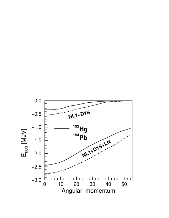
FIG. 6.: Total (proton + neutron) BCS-like pairing energies obtained for the lowest SD configurations in ¹⁹²Hg and ¹⁹⁴Pb in the calculations with (NL1+D1S+LN) and without (NL1+D1S) approximate particle number projection.

FIG. 7.: The dependence of the effective alignment $i_{eff}$ on the pairing and the particle number projection (panel (a)) and on the parametrization of the RMF Lagrangian (panel (b)). In both panels, the experimental data are shown by unlinked solid circles, while the results of the calculations by lines of different type. The experimental effective alignment between bands A and B is indicated as “A/B”. Band A in the lighter nucleus is taken as a reference, so the effective alignment measures the effect of the additional particle(s). In panel (a), the results of the calculations with no pairing (indicated as NL1 [CRMF]), without particle number projection (NL1+D1S) and with approximate particle number projection by means of the Lipkin-Nogami method (NL1+D1S+LN) are compared with the experimental effective alignment in the ¹⁹²Hg/¹⁹⁴Pb pair. Panel (b) compares effective alignments in the ¹⁹⁴Hg/¹⁹⁴Pb pair obtained with NL1 and NL3 forces with experimental data.

FIG. 8.: The dependence of the kinematic $(J^{(1)})$ and dynamic $(J^{(2)})$ moments of inertia of the lowest SD configurations in ¹⁹⁴Pb and ¹⁹⁴Hg on the parametrization of the RMF Lagrangian. The calculations have been performed with the sets NL1, NL3 and NLSH. In all calculations, the D1S set of parameters has been used for the Gogny force and approximate particle number projection has been performed by means of the Lipkin-Nogami method. Due to slow convergence the calculations with the NLSH set have been done only in the case of ¹⁹⁴Hg and only in the rotational frequency range $0.15-0.25$ MeV. In this frequency range the dynamic moment of inertia calculated with NLSH merge together with the ones obtained with NL3 and NL1 and thus it is not shown. No convergence is obtained in the calculations with NL3 above $\Omega_{x}>0.43$ MeV in the case of ¹⁹⁴Pb. Note that in the case of ¹⁹⁴Hg, the calculations with the NL3 force considerably overestimate the experimental dynamic moment of inertia in the band crossing region: the calculated value of $J^{(2)}$ reaches 202 MeV^-1 at 0.445 MeV. In panel (c), the proton contribution to $J^{(2)}$ is shown by a short-dashed line in order to make it more visible.

FIG. 9.: Transition quadrupole moments $Q_{t}$ and neutron and proton pairing energies $E_{pairing}$ of the lowest SD configurations in ¹⁹⁴Hg and ¹⁹⁴Pb shown in Fig. 8. The notation of lines is given there.

FIG. 10.: The dependence of the kinematic and dynamic moments of inertia of the lowest SD configuration in ¹⁹²Hg on the parametrization of the Gogny force. The results with the sets D1, D1P and D1S for the Gogny force are shown.

FIG. 11.: The dependence of the transition quadrupole moment $Q_{t}$ and neutron and proton pairing energies $E_{pairing}$ of the lowest SD configuration in ¹⁹²Hg on the parametrization of the Gogny force. The results with the sets D1, D1P and D1S for the Gogny force are shown.

FIG. 12.: Calculated and experimental dynamic and kinematic moments of inertia for yrast SD band in ¹⁹²Hg. Experimental data are shown by solid unlinked symbols. The calculations have been performed with scaling of the strength of the Gogny force: scaling factors 0.9, 1.0 and 1.1 have been used. Neutron and proton contributions into kinematic and dynamic moments of inertia are indicated by the letters $\nu$ and $\pi$, respectively

FIG. 13.: Transition quadrupole moments $Q_{t}$ and neutron and proton pairing energies $E_{pairing}$ of the lowest SD configuration in ¹⁹²Hg calculated with different scaling of the strength of the Gogny force. The notation of lines is given in the figure.

FIG. 14.: Dynamic moments of inertia $J^{(2)}$ of observed (solid circles) yrast SD bands in the ^190,192,194Hg and ^192,194,196Pb nuclei versus the ones of calculated lowest in energy SD configurations. Solid lines show the total calculated dynamic moments of inertia $J^{(2)}$, while long-dashed and dash-dotted lines show the contribution in $J^{(2)}$ from neutron and proton subsystems. The experimental data are taken from Refs. [75] (¹⁹²Pb), [69, 70, 71] (¹⁹⁴Pb), [78] (¹⁹⁶Pb), [76] (¹⁹⁰Hg), [77] (¹⁹²Hg) and [72, 73] (¹⁹⁴Hg).

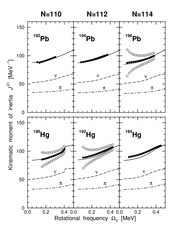
FIG. 15.: The same as Fig. 14 but for kinematic moments of inertia $J^{(1)}$. The experimental moments of inertia of linked or tentatively linked SD bands are shown by solid circles. In other cases (¹⁹⁶Pb, ^190,194Hg), the ’experimental’ kinematic moments of inertia $J^{(1)}$ are shown for three different spin values of the lowest state $I_{0}$ in the SD band, see text for details. The values being in best agreement with the calculations are indicated by solid circles, while open circles are used for alternatives.

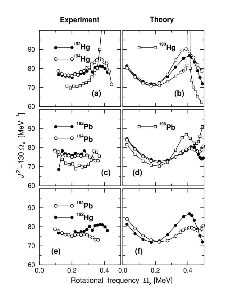
FIG. 16.: Comparison of experimental and calculated dynamic moments of inertia $J^{(2)}$ in the Hg (top panels) and the Pb (middle panels) isotopes as well as in the $N=112$ isotones (bottom panels). The same type of symbols is used for experimental bands (left panels) and their theoretical counterparts (right panels). In order to show the differences between different bands in more detail, the frequency dependent term is extracted from $J^{(2)}$, see text for details.

FIG. 17.: Effective alignments, $i_{eff}$ (in units $\hbar$), extracted from experiment (unlinked solid circles) are compared with those extracted from the corresponding calculated configurations (solid lines). Note that two absolute scales are used for the vertical axis. Panels b,c,f,g and i use the same scale with the difference between the lowest and the highest $i_{eff}$ values being $3\hbar$. On the other hand, the panels a,d and e use a scale with a difference of $1.5\hbar$.

FIG. 18.: Calculated neutron and proton pairing energies for the lowest SD configurations in ^192.194,196Pb and ^190,192,194Hg. Solid and dashed lines are used for neutrons and protons, respectively.

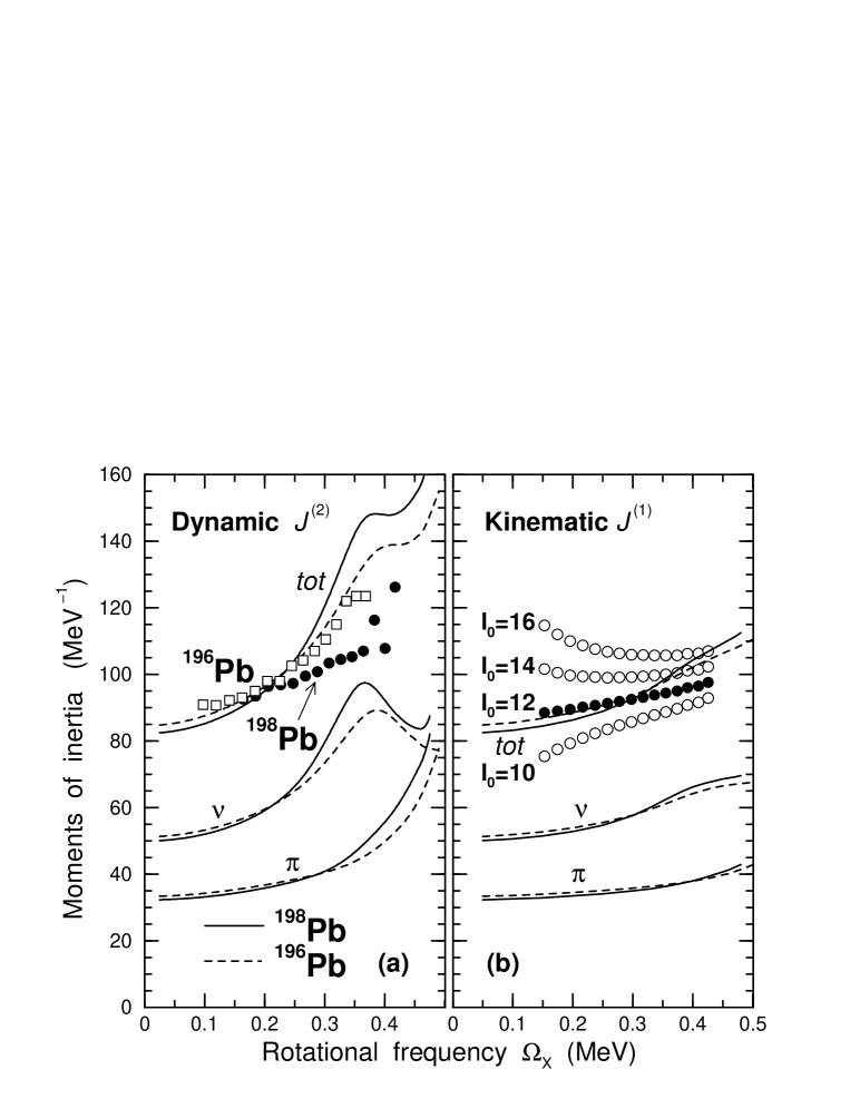
FIG. 19.: Calculated and experimental dynamic and kinematic moments of inertia for yrast SD band in ¹⁹⁸Pb. The results of the calculations are shown by solid lines. Experimental data for ¹⁹⁸Pb band is taken from Ref. [79] and ’experimental’ kinematic moments of inertia are shown for 4 different spin values for lowest state $I_{0}$. The $J^{(1)}$ values being in best agreement with results of the calculations at low spin are shown by solid circles. For comparison, the same quantities obtained for the lowest SD configuration in ¹⁹⁶Pb are shown by dashed lines. The experimental values of $J^{(2)}$ for yrast SD band in ¹⁹⁶Pb are shown by open squares.

FIG. 20.: Calculated transition quadrupole moments $Q_{t}$ and proton and neutron pairing energies $E_{pairing}$ of the lowest SD configuration in ¹⁹⁸Pb. For comparison, the same quantities obtained for the lowest SD configuration in ¹⁹⁶Pb are shown by dashed lines.

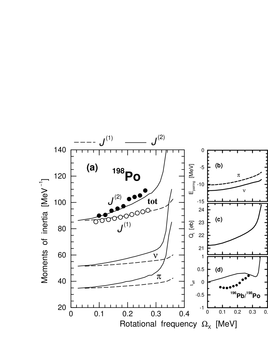
FIG. 21.: The results of the calculations for the lowest SD configuration in ¹⁹⁸Po. Dynamic and kinematic moments of inertia, proton and neutron pairing energies $E_{pairing}$, transition quadrupole moment $Q_{t}$ and effective alignment $i_{eff}$ in the ¹⁹⁶Pb/¹⁹⁸Po pair are shown in panels (a), (b), (c) and (d) respectively. The experimental data for the kinematic and dynamic moments of inertia are taken from Ref. [80] and shown by unlinked open and solid circles in panel (a). In panel (d), the experimental effective alignment is shown by unlinked solid circles.

FIG. 22.: Quasiparticle routhians corresponding to the lowest SD configuration in ¹⁹⁸Po, see caption of Fig. 5 for details.

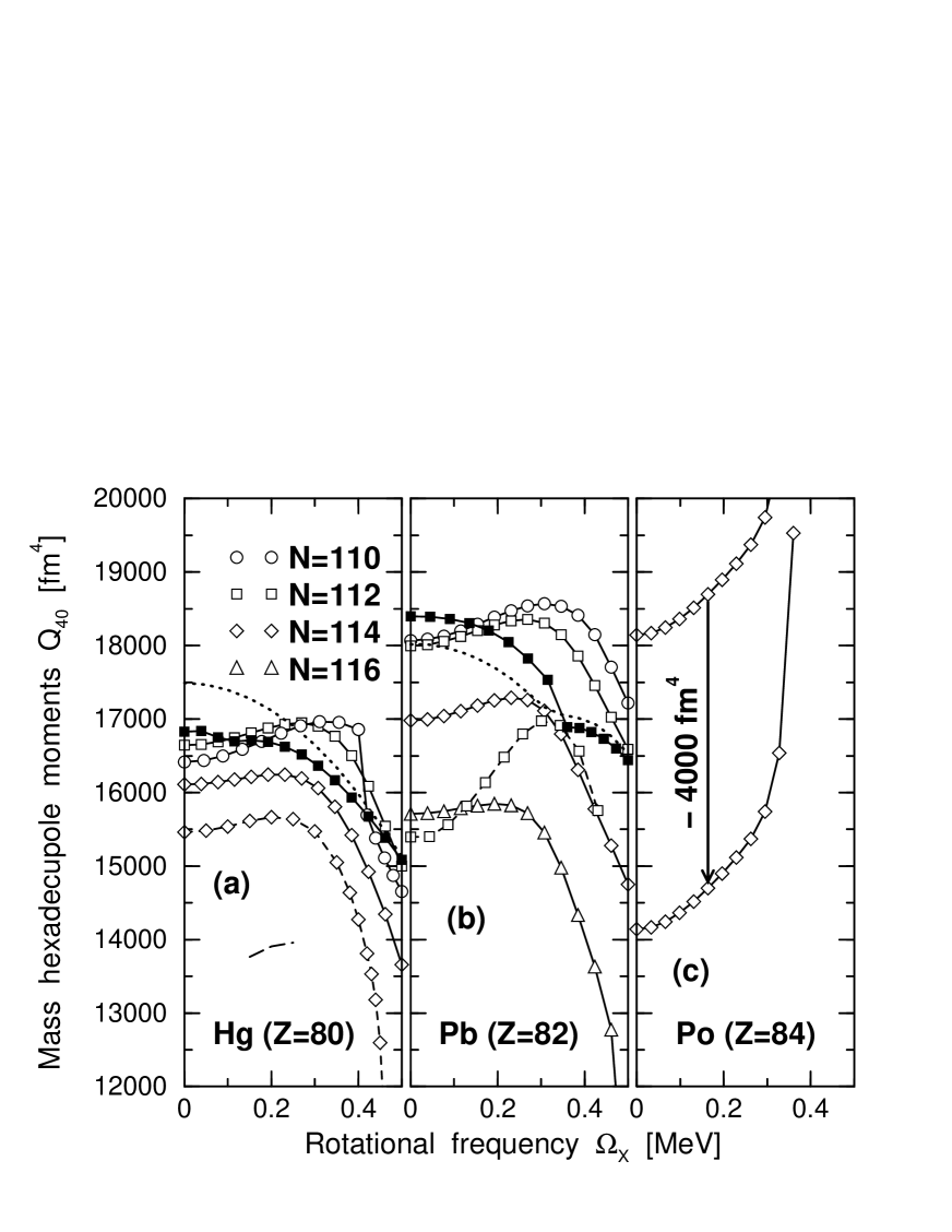
FIG. 23.: Calculated mass hexadecupole moments $Q_{40}$. Circles, squares, diamonds and triangles are used for the nuclei with $N=110$, 112, 114 and 116, respectively. Open symbols are used for the results of the calculations with APNP(LN), while filled symbols for the ones without APNP(LN). In panels (a) and (b), the results of the calculations without pairing are shown for ¹⁹²Hg and ¹⁹⁴Pb by dotted lines. Dashed lines are used to indicate the results obtained with the NL3 force, while long-dashed line in panel (a) shows the ones obtained in ¹⁹⁴Hg with the NLSH force. The lower curve in panel (c) is shifted down by $-4000$ fm⁴ relative to original (upper) curve in order to show the results of the calculations at high rotational frequencies.

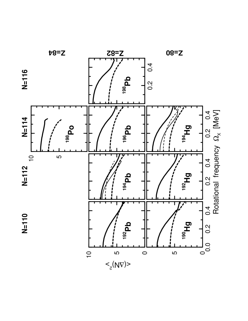
FIG. 24.: Particle number fluctuations $\langle(\hat{N})^{2}\rangle$ as a function of rotational frequency. Solid and dashed lines are used for neutrons and protons, respectively. Thick and thin lines are used for the values obtained with the forces NL1 and NL3, respectively.

TABLE I.: The values of the parameters of different sets for the finite range Gogny forces.

Parameter	D1S (Ref. [67])		D1P (Ref. [68])		D1 (Ref. [65])
$\mu_{i}$ (fm)	$0.7$	1.2	0.9	1.44	0.7	1.2
$W_{i}$	$-1720.30$	103.64	$-372.89$	34.62	$-402.4$	$-21.30$
$B_{i}$	1300.00	$-163.48$	62.69	$-14.08$	$-100.0$	$-11.77$
$H_{i}$	$-1813.53$	162.81	$-464.51$	70.95	$-496.2$	37.27
$M_{i}$	1397.60	$-223.93$	$-31.49$	$-20.96$	$-23.56$	$-68.81$

TABLE II.: The non-linear parameter sets NL1, NLSH and NL3. The masses are given in MeV, the parameter $g_{2}$ in $fm^{-1}$, while the rest of the parameters are dimensionless. The nuclear matter properties, predicted with these effectives forces, namely, the baryon density $\rho_{0}$ (in units $fm^{-3}$), the binding energy per particle $E/A$ (in MeV), the incompressibility $K$ (in MeV), the effective mass $m^{*}/m$ and the asymmetry parameter $J$ (in MeV) are also shown.

Parameter	NL1	NLSH	NL3
Masses
$m_{N}$	938.0	939.0	939.0
$m_{\sigma}$	492.25	526.059	508.194
$m_{\omega}$	795.36	783.0	782.501
$m_{\rho}$	763.0	763.0	763.0
Coupling constants
$g_{\sigma}$	10.138	10.4444	10.217
$g_{2}$	$-12.172$	$-6.9099$	$-10.431$
$g_{3}$	$-36.265$	$-15.8337$	$-28.885$
$g_{\omega}$	13.285	12.945	12.868
$g_{\rho}$	4.976	4.383	4.474
Nuclear matter properties
$\rho_{0}$	0.153	0.146	0.148
$E/A$	$-16.488$	$-16.346$	$-16.299$
$K$	211.29	355.36	271.76
$m^{*}/m$	0.57	0.60	0.60
$J$	43.7	36.1	37.4

TABLE III.: The spin assignment for the lowest state $I_{0}$ of the unlinked or tentatively linked [¹⁹²Pb] yrast SD bands. The lowest transition energies $E_{\gamma}(I_{0}+2\rightarrow I_{0})$ are also shown.

Nucleus	Ref.	$E_{\gamma}(I_{0}+2\rightarrow I_{0})$ [keV]	$I_{0}$
190Hg	[76]	316.9	$12^{+}$
192Hg	[77]	214.4	$8^{+}$
192Pb	[75]	214.8	$8^{+}$
196Pb	[78]	171.5	$6^{+}$
198Pb	[79]	305.1	$12^{+}$
198Po	[80]	175.9	$6^{+}$

REFERENCES

- [1] B. D. Serot and J. D. Walecka, Adv. Nucl. Phys. 16 (1986) 1.
- [2] J. N. Ginocchio, Phys. Rev. Lett. 78 (1997) 436.
- [3] P. Ring, Prog. Part. Nucl. Phys. 37 (1996) 193.
- [4] P. J. Twin, B. M. Nyakó, A. H. Nelson, J. Simpson, M. A. Bentley, H. W. Cranmer-Gordon, P. D. Forsyth, D. Howe, A. R. Mokhtar, J. D. Morrison, J. F. Sharpey-Schafer and G. Sletten, Phys. Rev. Lett. 57 (1986) 811.
- [5] D. R. Inglis, Phys. Rev. 96 (1954) 1059.
- [6] A. V. Afanasjev and P. Ring, report nucl-th/9909020, Physica Scripta, in press
- [7] J. Dobaczewski, Proc. of conf. “Nuclear structure 98”, Gatlinburg, Tennessee, USA, 1998, (Edited by C. Baktash), AIP 481, p. 315, (see also nucl-th/9811043).
- [8] W. Koepf and P. Ring, Nucl. Phys. A 493 (1989) 61.
- [9] W. Koepf and P. Ring, Nucl. Phys. A 511 (1990) 279.
- [10] J. König and P. Ring, Phys. Rev. Lett. 71 (1993) 3079.
- [11] A. V. Afanasjev, J. König and P. Ring, Nucl. Phys. A 608 (1996) 107.
- [12] A. V. Afanasjev, I. Ragnarsson and P. Ring, Phys. Rev. C 59 (1999) 3166.
- [13] C. E. Svensson, D. Rudolph, C. Baktash, M. A. Bentley, J. A. Cameron, M. P. Carpenter, M. Devlin, J. Eberth, S. Flibotte, A. Galindo-Uribarri, G. Hackman, D. S. Haslip, R. V. F. Janssens, D. R. LaFosse, T. J. Lampman, I. Y. Lee, F. Lerma, A. O. Macchiavelli, J. M. Nieminen, S. D. Paul, D. C. Radford, P. Reiter, L. L. Riedinger, D. G. Sarantites, B. Schaly, D. Seweryniak, O. Thelen, H. G. Thomas, J. C. Waddington, D. Ward, W. Weintraub, J. N. Wilson, C. H. Yu, A. V. Afanasjev, and I. Ragnarsson, Phys. Rev. Lett. 82 (1999) 3400.
- [14] M. Devlin, A. V. Afanasjev, R. M. Clark, D. R. LaFosse, I. Y. Lee, F. Lerma, A. O. Macchiavelli, R. W. MacLeod, I. Ragnarsson, P. Ring, D. Rudolph, D. G. Sarantites, and P. G. Thirolf, Phys. Rev. Lett. 82 (1999) 5217.
- [15] H. Madokoro and M. Matsuzaki, Prog. Theor. Phys. 101 (1999) 1027.
- [16] A. V. Afanasjev, J. König and P. Ring, Phys. Lett. B 367 (1996) 11.
- [17] A. V. Afanasjev, G. A. Lalazissis and P. Ring, Acta Phys. Hung. N. S. 6 (1997) 299.
- [18] A. V. Afanasjev, G. A. Lalazissis and P. Ring, Nucl. Phys. A 634 (1998) 395.
- [19] A. V. Afanasjev and P. Ring, Nucl. Phys. A 654 (1999) 647c.
- [20] A. V. Afanasjev, J. König and P. Ring, Phys. Rev. C 60 (1999) 051303.
- [21] J. Boguta and A. R. Bodmer, Nucl. Phys. A 292 (1977) 413.
- [22] P.-G. Reinhard, M. Rufa, J. Maruhn, W. Greiner and J. Friedrich, Z. Phys. A 323 (1986) 13.
- [23] J. L. Egido, H. J. Mang and P. Ring, Nucl. Phys. A 339 (1980) 390.
- [24] K. Kaneko, M. Nakano and M. Matsuzaki, Phys. Lett. B 317 (1993) 261.
- [25] H. Madokoro and M. Matsuzaki, Phys. Rev. C 56 (1997) R2934.
- [26] P. Ring, R. Beck and H. J. Mang, Z. Phys. 231 (1970) 10.
- [27] H. J. Mang, Phys. Rep. 18 (1975) 325.
- [28] P. Ring and P. Schuck, The Nuclear Many-Body Problem, (Springer Verlag, Heidelberg, 1980).
- [29] U. Hofmann and P. Ring, Phys. Lett. B 214 (1988) 307.
- [30] H. Kurcharek and P. Ring, Z. Phys. A 339 (1991) 23.
- [31] F. B. Guimaraes, B. V. Carlsson and T. Frederico, Phys. Rev. C 54 (1996) 2385.
- [32] F. Matera, G. Fabbri and A. Dellafiore, Phys. Rev. C 56 (1997) 228.
- [33] T. Gonzales-Llarena, J. L. Egido, G. A. Lalazissis and P. Ring, Phys. Lett. B 379 (1996) 13.
- [34] J. F. Berger, M. Girod and D. Gogny, Nucl. Phys. A 428 (1984) 23c.
- [35] A. Valor, J. L. Egido and L. M. Robledo, Nucl. Phys. in press (see also report nucl-th/9911027).
- [36] J. L. Egido and P. Ring, Nucl. Phys. A 383 (1982) 189; A 388 (1982) 19.
- [37] H. J. Lipkin, Ann. Phys. 9 (1960) 272.
- [38] Y. Nogami, Phys. Rev. 134 (1964) 313.
- [39] Y. Nogami and I. L. Zucker, Nucl. Phys. 60 (1964) 203.
- [40] H. C. Pradhan, Y. Nogami, and J. Law, Nucl. Phys. A 201 (1973) 357.
- [41] B. Gall, P. Bonche, J. Dobaczewski, H. Flocard and P.-H. Heenen, Z. Phys. A 348 (1994) 183.
- [42] J. Terasaki, P.-H. Heenen, P. Bonche, J. Dobaczewski and H. Flocard, Nucl. Phys. A 593 (1995) 1.
- [43] M. Girod, J. P. Delaroche, J. F. Berger, S. Peru and J. Libert, Z. Phys. A 358 (1997) 177.
- [44] A. Valor, J. L. Egido and L. M. Robledo, Phys. Lett. B 392 (1997) 249.
- [45] A. Villafranca and J. L. Egido, Phys. Lett. B 408 (1997) 35.
- [46] W. Satuła and R. Wyss, Phys. Rev. C 50 (1994) 2888.
- [47] W. Satuła, R. Wyss and P. Magierski, Nucl. Phys. A 578 (1994) 45.
- [48] A. V. Afanasjev, J. König, P. Ring, J. L. Egido and L. M. Robledo, to be published.
- [49] A. Kamlah, Z. Phys. 216 (1968) 52.
- [50] A. Valor, J. L. Egido and L. M. Robledo, Nucl. Phys., in press, (see also nucl-th/9911029).
- [51] J. König, PhD thesis, Physik-Department der Technischen Universität München, 1996.
- [52] A. V. Afanasjev, D. B. Fossan, G. J. Lane and I. Ragnarsson, Physics Reports 322 (1999) 1.
- [53] P. Ring, A. Hayashi, K. Hara, H. Emling and E. Grosse, Phys. Lett. B110 (1982) 423.
- [54] W. Nazarewicz and I. Ragnarsson, Nuclear deformations, in Handbook on nuclear properties, eds. D. N. Poenaru and W. Greiner (Claredon Press, Oxford, 1996) p. 80.
- [55] I. Ragnarsson, Phys. Lett. B 264 (1991) 5.
- [56] I. Ragnarsson, Nucl. Phys. A 557 (1993) 167c.
- [57] A. V. Afanasjev and I. Ragnarsson, Nucl. Phys. A 628 (1998) 580.
- [58] G. A. Lalazissis and P. Ring, Phys. Lett. B 427 (1998) 225.
- [59] M. A. Riley, D. M. Cullen, A. Alderson, I. Ali, P. Fallon, P. D. Forsyth, F. Hanna, S. M. Mullins, J. W. Roberts, J. F. Sharpey-Schafer, P. J. Twin, R. Poynter, R. Wadsworth, M. A. Bentley, A. M. Bruce, J. Simpson, G. Sletten, W. Nazarewicz, T. Bengtsson and R. Wyss, Nucl. Phys. A 512 (1990) 178.
- [60] J. Libert, M. Girod and J.-P. Delaroche, Phys. Rev. C 60 (1999) 054301.
- [61] B. Haas, V. P. Janzen, D. Ward, H. R. Andrews, D. C. Radford, D. Prévost, J. A. Kuehner, A. Omar, J. C. Waddington, T. E. Drake, A. Galindo-Uribarri, G. Zwartz, S. Flibotte, P. Taras and I. Ragnarsson, Nucl. Phys. A 561 (1993) 251.
- [62] G. A. Lalazissis, J. König and P. Ring, Phys. Rev. C 55 (1997) 540.
- [63] M. M. Sharma, M. A. Nagarajan and P. Ring, Phys. Lett. B 312 (1993) 377.
- [64] S. G. Nilsson and O. Prior, Mat. Fys. Medd. Dan. Vid. Selsk. 32 (1961) No.16.
- [65] D. Gogny, in Nuclear self-consistent fields, proceedings of the International conference held at the center for Theoretical Physics, Trieste, Italy, 1975, edited by G. Ripka and M. Porneuf (North-Holland, Amsterdam, 1975), p. 333.
- [66] J. Dechargé and D. Gogny, Phys. Rev. C 21 (1980) 1568.
- [67] J. F. Berger, M. Girod and D. Gogny, Comp. Phys. Comm. 63 (1991) 365.
- [68] M. Farine, D. Von-Eiff, P. Schuck, J. F. Berger, J. Dechargé and M. Girod, J. Phys. G 25 (1999) 863.
- [69] B. J. P. Gall, I. Deloncle, M.-G. Porquet, F. Hannachi, M. Aïiche, F. Azaiez, G. Bastin, C. W. Beausang, R. Beraud, C. Bourgeois, R. M. Clark, R. Duffait, J. Duprat, K. Hauschild, H. Hübel, M. J. Joyce, M. Kaci, A. Korichi, Y. Le Coz, M. Meyer, E. S. Paul, N. Perrin, N. Poffe, N. Redon, C. Schück, H. Sergolle, J. F. Sharpey-Schafer, J. Simpson, A. G. Smith and R. Wadsworth, Phys. Lett. B 345 (1995) 124.
- [70] A. Lopez-Martens, F. Hannachi, A. Korichi, C. Schück, E. Gueorguieva, Ch. Vieu, B. Haas, R. Lucas, A. Astier, G. Baldsiefen, M. Carpenter, G. de France, R. Duffait, L. Ducroux, Y. Le Coz, Ch. Finck, A. Gorgen, H. Hübel, T. L. Khoo, T. Lauritsen, M. Meyer, D. Prevost, N. Redon, C. Rigollet, H. Savajols, J. F. Sharpey-Schafer, O. Stezowski, Ch. Theisen, U. Van Severen, J. P. Vivien and A. N. Wilson, Phys. Lett. B 380 (1996) 18.
- [71] K. Hauschild, L. A. Bernstein, J. A. Becker, D. E. Archer, R. W. Bauer, D. P. McNabb, J. A. Cizewski, K.-Y. Ding, W. Younes, R. Krücken, R. M. Diamond, R. M. Clark, P. Fallon, I.-Y. Lee, A. O. Macchiavelli, R. MacLeod, C. J. Schmid, M. A. Deleplanque, F. S. Stephens and W. H. Kelly, Phys. Rev. C 55 (1997) 2819.
- [72] B. Cederwall, R. V. F. Janssens, M. J. Brinkman, I. Y. Lee, I. Ahmad, J. A. Becker, M. P. Carpenter, B. Crowell, M. A. Deleplanque, R. M. Diamond, J. E. Draper, C. Duyar, P. Fallon, L. P. Farris, E. A. Henry, R. G. Henry, J. R. Hughes, T. L. Khoo, T. Lauritsen, A. O. Macchiavelli, E. Rubel, F. S. Stephens, M. A. Stoyer, W. Satuła, I. Wiedenhoever and R. Wyss, Phys. Rev. Lett. 72 (1994) 3150.
- [73] T. L. Khoo, M. P. Carpenter, T. Lauritsen, D. Ackerman, I. Ahmad, D. J. Blumenthal, S. M. Fischer, R. V. F. Janssens, D. Nisius, E. F. Moore, A. Lopez-Martens, T. Døssing, R. Kruecken, S. J. Asztalos, J. A. Becker, L. Bernstein, R. M. Clark, M. A. Deleplanque, R. M. Diamond, P. Fallon, L. P. Farris, F. Hannachi, E. A. Henry, A. Korichi, I. Y. Lee, A. O. Macchiavelli and F. S. Stephens, Phys. Rev. Lett. 76 (1996) 1583.
- [74] G. Hackman, T. L. Khoo, M. P. Carpenter, T. Lauritsen, A. Lopez-Martens, I. J. Calderin, R. V. F. Janssens, D. Ackermann, I. Ahmad, S. Agarwala, D. J. Blumenthal, S. M. Fischer, D. Nisius, P. Reiter, J. Young, H. Amro, E. F. Moore, F. Hannachi, A. Korichi, I. Y. Lee, A. O. Macchiavelli, T. Døssing and T. Nakatsukasa, Phys. Rev. Lett. 79 (1997) 4100.
- [75] D. P. McNabb, J. A. Cizewski, K. Y. Ding, N. Fotiades, D. E. Archer, J. A. Becker, L. A. Bernstein, K. Hauschild, W. Younes, R. M. Clark, P. Fallon, I. Y. Lee, A. O. Macchiavelli and R. W. MacLeod, Phys. Rev. C 56 (1997) 2474.
- [76] A. N. Wilson, J. Timar, J. F. Sharpey-Schafer, B. Crowell, M. P. Carpenter, R. V. F. Janssens, D. J. Blumenthal, I. Ahmad, A. Astier, F. Azaiez, M. Bergström, L. Ducroux, B. J. P. Gall, F. Hannachi, T. L. Khoo, A. Korichi, T. Lauritsen, A. Lopez-Martens, M. Meyer, D. Nisius, E. S. Paul, M. G. Porquet, N. Redon, J. N. Wilson and T. Nakatsukasa, Phys. Rev. C 54 (1996) 559.
- [77] P. Fallon, T. Lauritsen, I. Ahmad, M. P. Carpenter, B. Cederwall, R. M. Clark, B. Crowell, M. A. Deleplanque, R. M. Diamond, B. Gall, F. Hannachi, R. G. Henry, R. V. F. Janssens, T. L. Khoo, A. Korichi, I. Y. Lee, A. O. Macchiavelli, C. Schuck and F. S. Stephens, Phys. Rev. C 51 (1995) R1609.
- [78] U. J. van Severen, W. Korten, H. Hübel, D. Bazzacco, G. LoBianco, N. H. Medina, C. Rossi Alvarez, S. Signorelli, K. Strähle and P. Willsau, Z. Phys. A 353 (1995) 15.
- [79] I. M. Hibbert, R. Wadsworth, K. Hauschild, H. Hübel, W. Korten, U. J. van Severen, E. S. Paul, A. N. Wilson, J. N. Wilson, A. P. Byrne, W. Satuła and R. Wyss, Phys. Rev. C 54 (1996) 2253.
- [80] D. P. McNabb, G. Baldsiefen, L. A. Bernstein, J. A. Cizewski, H.-Q. Jin, W. Younes, J. A. Becker, L. P. Farris, E. A. Henry, J. R. Hughes, C. S. Lee, S. J. Asztalos, B. Cederwall, R. M. Clark, M. A. Deleplanque, R. M. Diamond, P. Fallon, I. Y. Lee, A. O. Macchiavelli and F. S. Stephens, Phys. Rev. C 53 (1996) R541.
- [81] P. Magierski, S. Ćwiok, J. Dobaczewski, and W. Nazarewicz, Phys. Rev. C 48 (1993) 1686.
- [82] C. Baktash, B. Haas and W. Nazarewicz, Annu. Rev. Nucl. Part. Sci. 45 (1995) 485.
- [83] P. Fallon, P.-H. Heenen, W. Satuła, R. M. Clark, F. S. Stephens, M. A. Deleplanque, R. M. Diamond, I. Y. Lee, A. O. Macchiavelli and K. Vetter, Phys. Rev. C 60 (1999) 044301.