FZJ-IKP(TH)-2000-02 Ordinary and radiative muon capture on the proton
and the pseudoscalar form factor of the nucleon

Abstract

We calculate ordinary and radiative muon capture on the proton in an effective field theory of pions, nucleons and delta isobars, working to third and second order in the small scale expansion respectively. Preceding calculations in chiral effective field theories only employed pion and nucleon degrees of freedom and were not able to reproduce the photon spectrum in the pioneering experiment of radiative muon capture on the proton from TRIUMF. For the past few years it has been speculated that the discrepancy between theory and experiment might be due to $\Delta$(1232) related effects, which are only included via higher order contact interactions in the standard chiral approach. In this report we demonstrate that this speculation does not hold true. We show that contrary to expectations from naive dimensional analysis isobar effects on the photon spectrum and the total rate in radiative muon capture are of the order of a few percent, consistent with earlier findings in a more phenomenological approach. We further demonstrate that both ordinary and radiative muon capture constitute systems with a very well behaved chiral expansion, both in standard chiral perturbation theory and in the small scale expansion, and present some new ideas that might be at the bottom of the still unresolved discrepancy between theory and experiment in radiative muon capture. Finally we comment upon the procedure employed by the TRIUMF group to extract new information from their radiative muon capture experiment on the pseudoscalar form factor of the nucleon. We show that it is inconsistent with the ordinary muon capture data.

PACS: 23.40.-s,12.39.Fe,13.60-r

Keywords: Ordinary and radiative muon capture, pseudoscalar form factor, chiral effective field theory

I Introduction

With the ubiquitous success of the Standard Model ordinary and radiative muon capture on the proton can nowadays be considered as an excellent testing ground for our understanding of spontaneous and explicit chiral symmetry breaking in QCD. This stems from the fact that the typical momentum transfer in these reactions is very small—of the order of the muon mass—and one therefore can apply effective field theory methods, in particular baryon chiral perturbation theory.

Ordinary muon capture (OMC),

$$\mu^{-}(l)+p(r)\rightarrow\nu_{\mu}(l^{\prime})+n(r^{\prime})~{},$$ (1.1)

where we have indicated the four–momenta of the various particles, allows to measure the so–called induced pseudoscalar coupling constant, $g_{P}$. This coupling constant is nothing but the value of the induced pseudoscalar form factor $G_{P}(t)$ at the four–momentum transfer for muon capture by the proton at rest, $g_{p}=m_{\mu}\,G_{P}(t=-0.88m^{2}_{\mu})/2M_{N}$, with $m_{\mu}\,(M_{N})$ the muon (nucleon) mass. Theoretically, it is dominated by the pion pole as given by the time–honored PCAC prediction, $g_{P}^{\rm PCAC}=8.89$. Adler and Dothan [2] as well as Wolfenstein [3] calculated the first correction to the PCAC result utilizing by now outdated (and in some cases misleading) methods. The ADW relation was rederived directly from QCD Ward identities within the framework of heavy baryon chiral perturbation theory [4] and shown not to be affected by $\Delta(1232)$ effects in [5], $g_{P}^{\rm CHPT}=8.44\pm 0.23$ (a similar calculation with a slightly different result was given in [6]). The presently available data have, however, too large error bars to discriminate between the pion pole prediction and its corrected version [7]. Furthermore, $G_{p}(t)$ for low four–momentum transfer squared can be extracted from charged pion electroproduction measurements [8]. The resulting momentum dependence of the induced pseudoscalar form factor is in agreement with the pion pole prediction. However, as in the case of the pseudoscalar coupling, the data are not precise enough to be sensitive to the small corrections found in [2][3][4].

While the momentum transfer in OMC is fixed, radiative muon capture (RMC),

$$\mu^{-}(l)+p(r)\rightarrow\nu_{\mu}(l^{\prime})+n(r^{\prime})+\gamma(k)~{},$$ (1.2)

has a variable momentum transfer $t$ and one can get up to $t=m_{\mu}^{2}$ at the maximum photon energy of about $k\sim 100\,$MeV, which is quite close to the pion pole. This amounts approximately to a four times larger sensitivity to $g_{P}$ in RMC than OMC. However, this increased sensitivity is upset by the very small partial branching ratio in hydrogen $(\sim 10^{-8}$ for photons with $k>60\,$MeV) and one thus has to deal with large backgrounds. Precisely for this reason only very recently a first measurement of RMC on the proton has been published [9]. The resulting number for $g_{P}$, which was obtained using a relativistic tree model including the $\Delta$–isobar [10], came out significantly larger than expected from OMC, $g_{P}^{\rm RMC}=12.35\pm 0.88\pm 0.38=1.46\,g_{P}^{\rm CHPT}$. It should be noted that in this model the momentum dependence in $G_{P}(t)$ is solely given in terms of the pion pole and the induced pseudoscalar coupling is obtained as a multiplicative factor from direct comparison to the photon spectrum and the partial RMC branching ratio (for photon energies larger than 60 MeV). It was also argued in [9] that the atomic and molecular physics related to the binding of the muon in singlet and triplet atomic $\mu p$ and ortho and para $p\mu p$ molecular states is sufficiently well under control.

The TRIUMF result spurred a lot of theoretical activity. While radiative muon capture had already been calculated in phenomenological tree level models a long time ago, see e.g. [11][12][13][14][10], heavy baryon chiral perturbation theory was also used at tree level including dimension two operators [15] and to one loop order [16]. The resulting photon spectra are not very different from the ones obtained in the phenomenological models, the most striking feature being the smallness of the chiral loops [16], hinting towards a good convergence of the chiral expansion. At present, the puzzling result from the TRIUMF experiment remains unexplained. It is, however, a viable possibility that the discrepancy does not come from the strong interactions but rather is related to the distribution of the various spin states of the muonic atoms. It is therefore mandatory to sharpen the theoretical predictions for the strong as well as the non–strong physics entering the experimental analysis.

Here, we wish to reanalyze RMC in the framework of the so–called small scale expansion [19, 20], which allows to systematically include the $\Delta$ resonance into the effective field theory. Although Ando and Min [16] have already shown that the RMC process possesses a well behaved chiral expansion up to N²LO, it has been noted quite early [21] that one should reanalyze RMC in a chiral effective field theory with explicit $\Delta$ degrees of freedom. This is due to the fact that the $\Delta$-resonance lies quite close to the nucleon and therefore, in a delta-free theory like HBChPT as used in [16], could lead to unnaturally large higher order contact interactions which would spoil the seemingly good chiral convergence. Stating the same concern in the language of (naive) dimensional analysis, it suggests the possibility of corrections of the order of 30% due to the small nucleon–delta mass splitting, $m_{\mu}/(M_{\Delta}-M_{N})\sim 3m_{\mu}/M_{N}$. In the small scale expansion, the leading delta effects involving the large M1 $\gamma N\Delta$ vertex already appear at second order $\epsilon^{2}$ ($\epsilon$ denotes a genuine small parameter, the pion mass, external momentum or the $N\Delta$ mass splitting) and can therefore already be analyzed at tree level. The study presented here therefore constitutes a natural extension of the two previous analyses of RMC [15, 16] using chiral effective field theories. Some preliminary results where reported in ref.[23]. As we will show, the small scale expansion allows for a very transparent separation of the resonance and chiral pion effects.

The manuscript is organized as follows. In section 2, we briefly review how the Standard Model at low energies is mapped onto a chiral effective field theory. The ingredients of this field theory, which uses pions, nucleons and the delta isobar as degrees of freedom, are discussed in section 3. Section 4 is concerned with ordinary and radiative muon capture on the proton. In the framework of the small scale expansion in OMC the leading order delta effects only come in at N²LO (i.e. ${\cal O}(\epsilon^{3})$), whereas for RMC one can already study the explicit influence of this resonance at NLO (i.e. ${\cal O}(\epsilon^{2})$). The status of the induced pseudoscalar form factor is reviewed and the analysis of the TRIUMF RMC experiment is critically assessed in section 5. Section 6 contains the summary and conclusions. Some more technical aspects of this work are relegated to the appendix.

II From the Standard Model to the effective field theory

In this section we briefly summarize how QCD coupled to the standard electroweak theory is mapped onto the pertinent effective field theory. For that, we start with the electroweak Lagrangian. For our purpose, we only need the coupling of the charged currents to the charged massive gauge bosons $(W^{\pm}_{\mu}$) and the coupling of the massless photon ($A_{\mu}$) to the electromagnetic (em) current,

$${\cal L}_{\rm int}^{\rm SM}=-\frac{g_{2}}{\sqrt{8}}\left\{W_{\mu}^{+}(x)J_{\rm ch}^{\mu}+W_{\mu}^{-}(x)J_{\rm ch}^{\mu\dagger}\right\}-g_{1}\cos\theta_{W}A_{\mu}(x)J^{\mu}_{\rm em}+{\cal L}_{\rm ntl-wk}$$ (2.1)

where the last term refers to the non–leptonic weak interactions. $g_{1}$ and $g_{2}$ are the gauge couplings of the U(1)_Y and the SU(2)_L gauge groups and $\theta_{W}$ is the weak mixing (Weinberg) angle. In terms of the light quark and lepton fields the em and charged weak currents read

$$J_{\rm em}^{\mu} = \frac{2}{3}\bar{u}\gamma^{\mu}u-\frac{1}{3}\bar{d}\gamma^{\mu}d-\bar{\mu}\gamma^{\mu}\mu+\dots$$ (2.2)

$$J_{\rm ch}^{\mu} = \bar{u}_{w}\gamma^{\mu}\left(1-\gamma_{5}\right)d_{w}+\bar{\nu}_{\mu}\gamma^{\mu}\left(1-\gamma_{5}\right)\mu+\dots~{},$$ (2.3)

with $q_{w}=(u_{w},d_{w})$ denoting the quark eigenstates of the weak interaction and the ellipsis denoting terms we do not need in what follows. For constructing the effective field theory, it is most convenient to consider the QCD Lagrangian coupled to these gauge fields treated as external local sources, which transform locally under chiral symmetry [24]. With $e=g_{1}\cos\theta_{W}$ and $W_{\mu}^{-}={\cal V}_{\mu}^{-}(x)-{\cal A}_{\mu}^{-}(x)$, QCD coupled to these external sources takes the form

$${\cal L}_{\rm QCD}^{\rm ext.fields} = {\cal L}_{\rm QCD}^{0}+\bar{q}\left[\not{\bf v}(x)-\not{\bf a}(x)\gamma_{5}\right]q-\bar{q}\left[{\bf s}(x)-i\,{\bf p}(x)\right]q$$ (2.5)

$$+\bar{q}\left[\not{v}^{(0)}(x)-\not{a}^{(0)}(x)\gamma_{5}\right]q-\bar{q}\left[s^{(0)}(x)-i\,p^{(0)}(x)\right]q~{},$$

with $q$ the bi–spinor of the light quark fields in the strong interaction basis. For the case of RMC we are confronted with the following scenario of external sources:

$${\bf s}(x) = 0~{},$$ (2.6)

$$s^{(0)}(x) = \hat{m}\,I~{},$$ (2.7)

$${\bf p}(x) = p^{(0)}(x)\;=\;0~{},$$ (2.8)

$${\bf v}_{\mu}(x) = -e\,\frac{1}{2}\tau^{3}\,A_{\mu}(x)-\biggl{[}\frac{g_{2}V_{ud}}{\sqrt{8}}\left(\frac{1}{2}\tau^{1}-\frac{i}{2}\,\tau^{2}\right){\cal V}_{\mu}^{-}(x)+{\rm h.c.}\biggr{]}~{},$$ (2.9)

$$v_{\mu}^{(0)}(x) = -e\,\frac{1}{6}I\,A_{\mu}(x)~{},$$ (2.10)

$${\bf a}_{\mu}(x) = -\frac{g_{2}V_{ud}}{\sqrt{8}}\left(\frac{1}{2}\tau^{1}-\frac{i}{2}\,\tau^{2}\right){\cal A}_{\mu}^{-}(x)+{\rm h.c.}~{},$$ (2.11)

$$a_{\mu}^{(0)} = 0~{},$$ (2.12)

with $s(x),p(x),v_{\mu}(x)$ and $a_{\mu}(x)$ scalar, pseudoscalar, vector and axial–vector fields, in order, in an obvious isospin (singlet and triplet) notation. $V_{ud}$ is the pertinent element of the CKM matrix. Note that the term ${\cal L}_{\rm QCD}^{0}$ in Eq.(2.5) is chirally symmetric. The explicit chiral symmetry breaking due to the current quark masses resides in the zeroth component of the external scalar source.

Having specified the external field environment we now analyze the required strong matrix elements for calculating OMC and RMC. First we define quark vector and axial-vector currents

$$V_{\mu}^{a} = \bar{q}\,\gamma_{\mu}\,T^{a}\,q~{},$$ (2.13)

$$A_{\mu}^{a} = \bar{q}\,\gamma_{\mu}\gamma_{5}\,T^{a}\,q\;.$$ (2.14)

Here, the $T^{a}=\tau^{a}/2$ are the generators of SU(2). With these definitions one then specifies the strong matrix elements which have to be calculated in the effective theory

$$a)~{} \langle N|V_{\mu}^{a}|N\rangle~{},$$ (2.15)

$$b)~{} \langle N|A_{\mu}^{a}|N\rangle~{},$$ (2.16)

$$c)~{} \langle N|{\cal T}\,V_{\mu}^{a}V_{\nu}^{b}|N\rangle~{},$$ (2.17)

$$d)~{} \langle N|{\cal T}\,V_{\mu}^{a}A_{\nu}^{b}|N\rangle\;,$$ (2.18)

with all possible combinations of the external fields of Eqs.(2.6-2.12) and ${\cal T}$ denotes the conventional time–ordering operator. To proceed, we now have to specify the effective Lagrangian which will be used to calculate these matrix elements.

III Chiral Lagrangians

In this section, we briefly review the chiral Lagrangian underlying our calculation. While the meson part is standard, with the external momenta and the pion (light quark) mass counted as small parameters, for the meson–baryon system we include the nucleons as well as the $\Delta(1232)$ resonance. To systematically account for the effects of the latter, the $N\Delta$ mass splitting is considered as an additional small parameter. This is routed in phenomenology and the large $N_{c}$ limit of QCD, but not in the strict chiral limit, where the $\Delta$ decouples. These three small parameters are collectively denoted by $\epsilon$.

A Meson chiral perturbation theory

At low energies the chiral symmetry of QCD is spontaneously broken to the vectorial subgroup $SU(2)_{V}$: $SU(2)_{L}\times SU(2)_{R}\rightarrow SU(2)_{V}$. The strictures of the spontaneous and the explicit chiral symmetry breaking can be explored in terms of an effective field theory, chiral perturbation theory (ChPT). As a tool, one works with an effective Lagrangian, which consists of a string of terms with increasing dimension. For our purpose, we only need the first term in this expansion, the non-linear $\sigma$–model chirally coupled to the external sources,

$${\cal L}_{\pi\pi}^{(2)} = \frac{F_{0}^{2}}{4}\,{\rm Tr}\left[\nabla_{\mu}U^{\dagger}\nabla^{\mu}U+\chi^{\dagger}U+\chi U^{\dagger}\right]~{}$$ (3.1)

with

$$U(x) = \exp\left\{\frac{i}{F_{0}}\,\tau\cdot\pi(x)\right\}~{},$$ (3.2)

$$\nabla_{\mu}U = \partial_{\mu}U-i({\bf v_{\mu}}+{\bf a_{\mu}})U+iU({\bf v_{\mu}}-{\bf a_{\mu}})~{},$$ (3.3)

$$\chi = 2B_{0}\left({\bf s}+s^{(0)}+i\,{\bf p}+i\,p^{(0)}\right)~{}.$$ (3.4)

The pions, which are nothing but integration variables, are collected in the matrix–valued field $U(x)$ and the explicit symmetry breaking due to the light quark masses is hidden in $\chi$ via the zeroth component of the scalar source. $F_{0}$ is the (weak) pion decay constant (in the chiral limit) and $B_{0}$ is related to the scalar quark condensate. We work in the standard scenario with $B_{0}\gg F_{0}$. This specifies completely the meson part of the effective Lagrangian.

B Including baryons: The small scale expansion

The nucleon–delta–pion system chirally coupled to the external fields can also be represented by a Lagrangian, which decomposes into a string of terms with increasing dimension. We work here in the heavy mass formulation, in which the nucleon and the delta are essentially considered as heavy, static sources. This allows to shuffle the baryon mass ($M_{B}$) dependence into a string of $1/M_{B}$ suppressed vertices and gives rise to a consistent power counting [25][26][20]. Denoting by $N$ the (heavy) nucleon isodoublet field and by $T_{\mu}^{i}$ the Rarita–Schwinger representation of the heavy spin-3/2 field, the lowest order terms read

$${\cal L}_{\pi N}^{(1)} = \bar{N}\left[i\;v\cdot D\;+\;\dot{g}_{A}\;S\cdot u\right]N~{},$$ (3.5)

$${\cal L}_{\pi\Delta}^{(1)} = -\;\bar{T}^{\mu}_{i}\left[i\;v\cdot D^{ij}-\delta^{ij}\Delta_{0}+\ldots\right]\;g_{\mu\nu}\;T^{\nu}_{j}~{},$$ (3.6)

$${\cal L}_{\pi N\Delta}^{(1)} = \dot{g}_{\pi N\Delta}\;\left\{\bar{T}^{\mu}_{i}\;g_{\mu\alpha}\;w^{\alpha}_{i}\;N\;+\;\bar{N}\;w^{\alpha\dagger}_{i}\;g_{\alpha\mu}\;T^{\mu}_{i}\right\}~{},$$ (3.7)

with $\Delta_{0}=M_{\Delta}-M_{0}\,(M_{0})$ being the nucleon-delta mass splitting (nucleon mass) in the chiral limit (to the order we are working, we can set $\Delta_{0}=\Delta$). All other quantities $Q$ in the chiral limit are denoted as $\dot{Q}$. Furthermore, $v_{\mu}$ and $S_{\mu}$ are the four–velocity and the spin–vector of the heavy nucleon. The various chiral covariant derivatives, chiral connections and vielbeins are (for details, we refer to [27] and [20])

$$D_{\mu}N = (\partial_{\mu}+\Gamma_{\mu}-iv_{\mu}^{(s)})N~{},$$ (3.8)

$$v_{\mu}^{(s)} = 3\,v_{\mu}^{(0)}~{},$$ (3.9)

$$\Gamma_{\mu} = {1\over 2}[u^{\dagger},\partial_{\mu}u]-{i\over 2}u^{\dagger}({\bf v_{\mu}}+{\bf a_{\mu}})u-{i\over 2}u({\bf v_{\mu}}-{\bf a_{\mu}})u^{\dagger}\equiv\tau^{i}\;\Gamma_{\mu}^{i}~{},$$ (3.10)

$$u_{\mu} = iu^{\dagger}\nabla_{\mu}Uu^{\dagger}\equiv\tau^{i}\;w_{\mu}^{i}~{},$$ (3.11)

$$D_{\mu}^{ij}T_{\nu}^{j} = \left(\partial_{\mu}\delta^{ij}+C_{\mu}^{ij}\right)T_{\nu}^{j}~{},$$ (3.12)

$$C^{ij}_{\mu} = \delta^{ij}\left(\Gamma_{\mu}-iv^{(s)}_{\mu}\right)-2i\epsilon^{ijk}\Gamma^{k}_{\mu}~{},$$ (3.13)

where $i,j,k$ are isospin indices. At second order in the small scale expansion, we need the following terms

$${\cal L}_{\pi N}^{(2)} = {1\over 2M_{0}}\bar{N}\left\{(v\cdot D)^{2}-D^{2}-ig_{A}\left(S\cdot D\,v\cdot u+v\cdot u\,S\cdot D\right)\right.$$ (3.15)

$$\phantom{{1\over 2M_{0}}\bar{N}}\left.-\frac{i}{2}\left[S^{\mu},S^{\nu}\right]_{-}\left[\left(1+\dot{\kappa}_{v}\right)f_{\mu\nu}^{+}+2\left(1+\dot{\kappa}_{s}\right)v_{\mu\nu}^{(s)}\right]+\dots\right\}N~{},$$

$${\cal L}_{\pi N\Delta}^{(2)} = \bar{T}^{\mu}_{i}\;\frac{1}{2M_{0}}\left[b_{1}\;if_{+\mu\nu}^{\;i}S^{\nu}+\ldots\right]N+{\rm h.c.}$$ (3.16)

with

$$f_{\mu\nu}^{\pm} = u^{\dagger}F_{\mu\nu}^{R}u\pm uF_{\mu\nu}^{L}u^{\dagger}\equiv\tau^{i}\;f_{\pm\mu\nu}^{i}\;,$$ (3.17)

$$F_{\mu\nu}^{X} = \partial_{\mu}F_{\nu}^{X}-\partial_{\nu}F_{\mu}^{X}-i\left[F_{\mu}^{X},F_{\nu}^{X}\right];\;\;X=L,R\;,$$ (3.18)

$$F_{\mu}^{R} = {\bf v_{\mu}}+{\bf a_{\mu}}\;,\hskip 14.22636ptF_{\mu}^{L}\;=\;{\bf v_{\mu}}-{\bf a_{\mu}}\;,$$ (3.19)

$$v_{\mu\nu}^{(s)} = \partial_{\mu}v_{\nu}^{(s)}-\partial_{\nu}v_{\mu}^{(s)}\;.$$ (3.20)

Note that in ${\cal L}_{\pi N}^{(2)}$ only two low–energy constants (LECs) appear, which we have expressed in terms of the isoscalar and isovector anomalous magnetic moments, $\kappa_{s}$ and $\kappa_{v}$, of the nucleon, respectively. The LEC $b_{1}$ is fixed from neutral pion photoproduction at threshold, $b_{1}=12.0$. The ${\cal O}(\epsilon^{2})$ Lagrangians given so far are sufficient to calculate the leading order $\Delta$(1232) effects in RMC. However, as mentioned above, in OMC the leading $\Delta$(1232) related effects only occur at N²LO—specifically as a ${\cal O}(\epsilon^{3})$ contribution to the form factors of the nucleon. In SSE these terms have already been calculated in [5] and we refer the reader interested in the details of the third order Lagrangian required for such a calculation to ref.[5]. We now have specified the effective Lagrangian needed to work out OMC and RMC to second order in the small scale expansion. The pertinent Feynman rules to perform these calculations are collected in appendix A.

IV Muon capture

This section is concerned with the theoretical description of OMC and RMC. To keep the manuscript self–contained, we give all formulae necessary to calculate the capture rates.

A Leptonic matrix elements

Consider first the purely leptonic part of the muon capture reaction. For OMC and RMC, we need the following two leptonic matrix elements:

$$\langle\nu_{\mu}|J_{\mu}^{+}|\mu\rangle = -i\,\frac{g_{2}}{\sqrt{8}}\,\bar{\nu}_{\mu}(l^{\prime})\gamma_{\mu}\left(1-\gamma_{5}\right)\mu(l)~{},$$ (4.1)

$$\langle\nu_{\mu}\,\gamma|J_{\mu}^{+}|\mu\rangle = -i\,\frac{g_{2}}{\sqrt{8}}\,\frac{e}{2l\cdot k}\,\bar{\nu}_{\mu}(l^{\prime})\gamma_{\mu}\left(1-\gamma_{5}\right)\left(2\epsilon^{\ast}\cdot l-\not{k}\not{\epsilon}^{\ast}\right)\mu(l)~{},$$ (4.2)

with $\epsilon^{\ast}_{\mu}$ the polarization vector of the photon. The corresponding four–momenta have already been defined in Eq.(1.1) and Eq.(1.2), respectively.

B Hadronic matrix elements

For OMC one only needs to calculate the vector and axial-vector transition matrix elements $\langle n|V_{\mu}^{-}|p\rangle,\;\langle n|A_{\mu}^{-}|p\rangle$ of Eqs.(2.15,2.16). In the limit of exact isospin symmetry these matrix-elements constitute the off-diagonal components of the isovector nucleon vector and axial-vector currents which are typically parameterized in terms of four form factors (e.g. ref.[5]): the isovector vector form factors $F_{1,2}^{v}$, as well as the axial and the induced pseudoscalar form factor, $G_{A}(q^{2})$ and $G_{P}(q^{2})$ respectively. In terms of these, the relativistic strong matrix elements defined in Eqs.(2.15,2.16) (which corresponds to the vector and axial correlators, shown in the first row of fig.1) are given by:

$$\langle n|V_{\mu}^{-}|p\rangle = -i\,\frac{g_{2}V_{ud}}{\sqrt{8}}\,\bar{n}(p_{2})\left[F_{1}^{v}(q^{2})\gamma_{\mu}+\frac{i}{2M_{N}}F_{2}^{v}(q^{2})\sigma_{\mu\nu}q^{\nu}\right]p(p_{1})~{},$$ (4.3)

$$\langle n|A_{\mu}^{-}|p\rangle = -i\,\frac{g_{2}V_{ud}}{\sqrt{8}}\,\bar{n}(p_{2})\left[G_{A}(q^{2})\gamma_{\mu}\gamma_{5}+\frac{G_{P}(q^{2})}{2M_{N}}q_{\mu}\gamma_{5}\right]p(p_{1}).$$ (4.4)

where $q^{2}=(p_{2}-p_{1})^{2}$ is the invariant momentum transfer squared. The Dirac $F_{1}^{(v)}$ and Pauli $F_{2}^{(v)}$ form factor are subject to the normalizations

$$F_{1}^{(v)}(0)=1~{},\quad F_{2}^{(v)}(0)=\kappa_{v}~{},$$ (4.5)

with $\kappa_{v}=3.71$ the isovector nucleon anomalous magnetic moment. In the axial matrix element, Eq.(4.4) one has assumed the absence of second class currents. The electromagnetic form factor are rather well known. The current situation concerning their theoretical understanding and experimental knowledge can be found e.g. in [29]. Muon captures therefore provide us with the opportunity to study the weak axial structure of a nucleon. While $G_{A}(q^{2})$ can be extracted from (anti)neutrino–proton scattering or charged pion electroproduction data, $G_{P}(q^{2})$ is harder to pin down and in fact constitutes the least known nucleon form factor. In Fig.7 we present the “world data” for $G_{P}(q^{2})$.

These four form factors have already been calculated to ${\cal O}(\epsilon^{3})$ in [5]. One finds

$$F_{i}^{(v)}(q^{2}) = F_{i}^{(v)}(0)\left[1+\frac{1}{6}(r_{i}^{v})^{2}q^{2}+{\cal O}(q^{4})\right]$$ (4.6)

$$G_{A}(q^{2}) = g_{A}\left[1+\frac{1}{6}(r_{A})^{2}q^{2}+{\cal O}(q^{4})\right]$$ (4.7)

$$G_{P}(q^{2}) = \frac{4M_{N}g_{\pi NN}F_{\pi}}{m_{\pi}^{2}-q^{2}}-\frac{2}{3}g_{A}M_{N}^{2}r_{A}^{2}\;.$$ (4.8)

where we have systematically shifted all appearing quantities to their physical values. $r_{1,2}^{v}$ and $r_{A}$ are the isovector Dirac and Pauli radius and the axial radius respectively. They receive contributions from chiral loops and counter-terms, except for $r_{2}^{v}$ which is free of any LEC. Detailed results can be found in [5]. In Fig.7 the difference between the usual pion-pole parameterization for $G_{P}(q^{2})$ and the full chiral structure of the form factor, Eq.4.8 is displayed. Note that this chiral structure is not affected by $\Delta$(1232). In the kinematical region of RMC, which mainly lies to the “left” of the OMC point in Fig.7 the structure effect in $G_{P}(q^{2})$ proportional to the axial radius $r_{A}$ is expected to play only a small role. Certainly, the present experimental uncertainties both in OMC [7] and in RMC [9] are too large to distinguish between the two curves, but new efforts are under way [34].

Usually the non relativistic reduction of Eqs.(4.3,4.4) is done in the Breit frame. Here we give the non relativistic strong matrix elements in the rest frame of the proton where our calculation is done:

$$\langle n|V_{\mu}^{-}|p\rangle = -i\,\frac{g_{2}V_{ud}}{\sqrt{8}}\ {\cal N}_{2}\,\bar{n}_{v}(p_{2})\left\{\left(\frac{2M_{N}}{E_{2}+M_{N}}F_{1}^{(v)}(q^{2})-\frac{E_{2}-M_{N}}{E_{2}+M_{N}}F_{2}^{(v)}(q^{2})\right)v_{\mu}\right.$$ (4.11)

$$+\left[\frac{1}{E_{2}+M_{N}}\left(F_{1}^{(v)}(q^{2})+F_{2}^{(v)}(q^{2})\right)-\frac{1}{2M_{N}}F_{2}^{(v)}(q^{2})\right]q_{\mu}$$

$$\left.+\frac{2}{E_{2}+M_{N}}\left[S_{\mu},S\cdot q\right]\left(F_{1}^{(v)}(q^{2})+F_{2}^{(v)}(q^{2})\right)\right\}p_{v}(0)~{},$$

$$\langle n|A_{\mu}^{-}|p\rangle = -i\,\frac{g_{2}V_{ud}}{\sqrt{8}}\ {\cal N}_{2}\,\bar{n}_{v}(p_{2})\left\{G_{A}(q^{2})\left[2\,S_{\mu}-\frac{2\,S\cdot q\,v_{\mu}}{E_{2}+M_{N}}\right]\right.$$ (4.13)

$$\left.+R\,G_{P}(q^{2})\,\frac{S\cdot q\,q_{\mu}}{M_{N}\left(E_{2}+M_{N}\right)}\right\}p_{v}(0),$$

where ${\cal N}_{2}$ is the usual normalization factor of the neutron wave function, ${\cal N}_{2}=\sqrt{\frac{E_{2}+M_{N}}{2M_{N}}}$ and $E_{2}$ is the neutron energy. One gets immediately the results to ${\cal O}(\epsilon^{2})$ by replacing the form factors by their values at $q^{2}=0$

We now turn to the vector–vector (VV) and vector–axial (VA) correlator which we only need to ${\cal O}(\epsilon^{2})$ in SSE. Working in the Coulomb gauge $\epsilon^{\ast}\cdot v=0$ for the photon and making use of the transversality condition $\epsilon^{\ast}\cdot k=0$, we find (the pertinent Feynman diagrams for the VV correlator are shown in the second row in fig. 1 and the ones for VA in figs. 2,3)

$$\langle n|{\cal T}\,V\cdot\epsilon^{\ast}V_{\mu}^{-}|p\rangle^{(2)} = -i\,\frac{g_{2}V_{ud}\,e}{\sqrt{8}}\,\bar{n}_{v}(r^{\prime})\left\{\frac{1+\kappa_{v}}{M_{N}}\left[S_{\mu},S\cdot\epsilon^{\ast}\right]-\frac{1}{2M_{N}}\,\epsilon^{\ast}_{\mu}\right.$$ (4.15)

$$\phantom{-i\,\frac{g_{2}V_{ud}\,e}{\sqrt{8}}\,\bar{n}(r^{\prime})}\left.+\frac{1}{M_{N}\omega}\,v_{\mu}\left[\left(1+\kappa_{v}\right)[S\cdot\epsilon^{\ast},S\cdot k]-\epsilon^{\ast}\cdot r\right]+{\cal O}(1/M_{N}^{2})\right\}p_{v}(r)~{},$$

$$\langle n|{\cal T}\,V\cdot\epsilon^{\ast}A_{\mu}^{-}|p\rangle^{(2)} = -i\,\frac{g_{2}V_{ud}\,e}{\sqrt{8}}\,\bar{n}_{v}(r^{\prime})\times$$ (4.23)

$$\left\{2\,R\,g_{A}\,\frac{S\cdot(r^{\prime}-r)}{(r^{\prime}-r)^{2}-m_{\pi}^{2}}\times\left[\frac{2\,\epsilon^{\ast}\cdot(l-l^{\prime})\,(l-l^{\prime})_{\mu}}{(l-l^{\prime})^{2}-m_{\pi}^{2}}-\epsilon^{\ast}_{\mu}\right]\right.$$

$$-R\,\frac{g_{A}}{M_{N}}\,\frac{\left(v\cdot r^{\prime}-v\cdot r\right)S\cdot(r+r^{\prime})}{(r^{\prime}-r)^{2}-m_{\pi}^{2}}\times\left[\frac{2\,\epsilon^{\ast}\cdot(l-l^{\prime})\,(l-l^{\prime})_{\mu}}{(l-l^{\prime})^{2}-m_{\pi}^{2}}-\epsilon^{\ast}_{\mu}\right]$$

$$-2\,R\,g_{A}\left[1+\frac{v\cdot l-v\cdot l^{\prime}}{2M_{N}}\right]\frac{S\cdot\epsilon^{\ast}\,(l-l^{\prime})_{\mu}}{(l-l^{\prime})^{2}-m_{\pi}^{2}}+\frac{g_{A}}{M_{N}}\,S\cdot\epsilon^{\ast}\,v_{\mu}$$

$$+\frac{g_{A}}{M_{N}}\left[\frac{(2+\kappa_{s}+\kappa_{v})\,S^{\alpha}\,[S\cdot\epsilon^{\ast},S\cdot k]}{\omega}+\frac{(\kappa_{v}-\kappa_{s})\,[S\cdot\epsilon^{\ast},S\cdot k]\,S^{\alpha}}{\omega}\right.$$

$$\phantom{+\frac{g_{A}}{M_{N}}}\left.-\frac{2\,S^{\alpha}\epsilon^{\ast}\cdot r}{\omega}\right]\times\left[g_{\mu\alpha}-R\,\frac{(l-l^{\prime})_{\alpha}(l-l^{\prime})_{\mu}}{(l-l^{\prime})^{2}-m_{\pi}^{2}}\right]$$

$$+\frac{g_{\pi N\Delta}b_{1}}{3\,M_{N}}\left[\frac{2\Delta\,[k^{\alpha}S\cdot\epsilon^{\ast}-\omega\,v^{\alpha}S\cdot\epsilon^{\ast}-\epsilon^{\ast\,\alpha}S\cdot k]}{\Delta^{2}-\omega^{2}}-\frac{4\,S^{\alpha}[S\cdot\epsilon^{\ast},S\cdot k]}{3\,(\Delta+\omega)}\right.$$

$$\phantom{+\frac{g_{\pi N\Delta}b_{1}}{3\,M_{N}}}\left.\left.+\frac{4\,[S\cdot\epsilon^{\ast},S\cdot k]\,S^{\alpha}}{3\,(\Delta-\omega)}\right]\times\left[g_{\mu\alpha}-\frac{(l-l^{\prime})_{\alpha}(l-l^{\prime})_{\mu}}{(l-l^{\prime})^{2}-m_{\pi}^{2}}\right]+{\cal O}(1/M_{N}^{2})\right\}p_{v}(r)~{},$$

with $\omega=v\cdot k$ and $R=1$ in QCD. We have introduced this factor multiplying the Born term contributions proportional to the induced pseudoscalar form factor for the later discussion. One can easily check from the continuity equations satisfied by the correlators (which for example relates the vector–axial correlator to the axial one, see [22]) that gauge invariance is satisfied in the above equations. We note again that here we only give the results to ${\cal O}(\epsilon^{2})$ as this is sufficient to study the leading order $\Delta$(1232) effects in RMC. We also want to point out that the vector–vector correlator is free of delta effects to this order ${\cal O}(\epsilon^{2})$, i.e. the leading $\Delta$(1232) effect only appears in the vector–axial correlator, cf. fig 3.

C Ordinary Muon Capture

Surprisingly, no full analysis of OMC exists in the literature for the framework of chiral effective field theories. All previous analyses [4, 5, 6] stopped at the level of writing down the relevant matrix-elements/form factors (here Eqs.(4.3,4.4)), but no discussion of the implications for the lifetime of OMC was given, which can be written down in a closed analytic form. In this section we are going to fill this gap. We work in the Fermi approximation of a static $W_{\mu}^{-}$ field, i.e. the gauge boson propagator is reduced to a point interaction (since the typical momenta involved are much smaller than the $W$ mass),

$${\cal M}_{\mu^{-}p\rightarrow\nu_{\mu}n} = {\cal M}^{\rm OMC}=\langle\nu_{\mu}|W_{\mu}^{+}|\mu\rangle\,i\,\frac{g^{\mu\nu}}{M_{W}^{2}}\left[\langle n|V_{\nu}^{-}|p\rangle-\langle n|A_{\nu}^{-}|p\rangle\right]~{}.$$ (4.24)

1 Spin-averaged OMC

Introducing the Fermi constant $G_{F}$ via $G_{F}={g_{2}^{2}\sqrt{2}}/{(8M_{W}^{2})}$, we define the square of the spin-averaged invariant matrix element to be

$$\frac{1}{4}\sum_{\sigma\sigma^{\prime}ss^{\prime}}|{\cal M}^{\rm OMC}|^{2} = \frac{G_{F}^{2}V_{ud}^{2}}{2}\,L_{\mu\nu}^{(a)}H^{\mu\nu}_{(a)}\;.$$ (4.25)

With the normalizations

$$\sum_{s}\mu(l,s)\bar{\mu}(l,s)=\frac{\not{l}+m_{\mu^{-}}}{2\,m_{\mu^{-}}}, \quad\sum_{s}\nu(l^{\prime},s)\bar{\nu}(l^{\prime},s)=\not{l}^{\prime},$$ (4.26)

$$\sum_{\sigma}p_{v}(r,\sigma)\bar{p}_{v}(r,\sigma)=P_{v}^{+}\left(1+\frac{v\cdot r}{2M_{N}}\right),\quad \sum_{\sigma}n_{v}(r^{\prime},\sigma)\bar{n}_{v}(r^{\prime},\sigma)=P_{v}^{+}\left(1+\frac{v\cdot r^{\prime}}{2M_{N}}\right),$$ (4.27)

one then obtains the symmetric tensors

$$L_{\mu\nu}^{(a)} = \frac{2}{m_{\mu^{-}}}\left\{l_{\mu}l^{\prime}_{\nu}-g_{\mu\nu}l\cdot l^{\prime}+l^{\prime}_{\mu}l_{\nu}+i\epsilon_{\mu\alpha\nu\beta}l^{\alpha}l^{\prime\beta}\right\}~{},$$ (4.28)

$$H_{\mu\nu}^{(a)} = av_{\mu}v_{\nu}+b\left(v_{\mu}v_{\nu}-g_{\mu\nu}\right)+c\,r^{\prime}_{\mu}r^{\prime}_{\nu}+d\,\left(v_{\mu}r^{\prime}_{\nu}+r^{\prime}_{\mu}v_{\nu}\right)+e\,i\epsilon_{\mu\nu}^{\alpha\beta}r^{\prime}_{\alpha}v_{\beta}~{}.$$ (4.29)

Note that we have evaluated the tensors for the special kinematic condition of both the proton and the muon being at rest, i.e. $l_{\mu}=(m_{\mu^{-}},0,0,0),\;r_{\mu}=(0,0,0,0)$. $a,b,c,d,e$ are coefficients which depend on the four form factors Eqs.(4.6, 4.7). For illustration we give them to ${\cal O}(\epsilon^{2})$

$$a=1\,,\quad b=g_{A}^{2}\,,\quad c=-g_{A}^{2}\frac{\vec{r}^{\,\prime\,2}+2m_{\pi}^{2}}{(\vec{r}^{\,\prime\,2}+m_{\pi}^{2})^{2}}\,,\quad d=\frac{1+g_{A}^{2}}{2M_{N}}\,,\quad e=\frac{g_{A}(1+\kappa_{v})}{M_{N}}~{}.$$ (4.30)

We now assume that the initial muon-proton system constitutes the ground-state of a bound system. We therefore replace the plane-wave wavefunction of the muon used so far in the calculation by the 1s Bohr-wavefunction $\Phi(x)_{1s}$ of a muonic atom. We note that to ${\cal O}(\epsilon^{2})$ we are not sensitive to the extended structure of the proton – any dependence of the capture process on the electric/magnetic radius of the nucleon will only occur at ${\cal O}(\epsilon^{3})$ [5]. As we will see below, the terms of ${\cal O}(\epsilon^{3})$ in OMC only represent a small N²LO correction. For simplicity we therefore approximate the muonic atom wave-function dependence by its value at the origin even at ${\cal O}(\epsilon^{3})$, which effectively constitutes an upper bound for the ${\cal O}(\epsilon^{3})$ correction to the total width. In a systematic ${\cal O}(\epsilon^{3})$ analysis one would of course have to calculate the overlap between the Bohr-wavefunction and the respective proton-neutron transition form factors. Confining ourselves to $x=0$ we use

$$\Phi(0)_{1s}=\frac{\alpha^{3/2}\mu^{3/2}}{\sqrt{\pi}}\;,$$ (4.31)

with the reduced mass $\mu={M_{N}m_{\mu^{-}}}/{(M_{N}+m_{\mu^{-}})}$ and $\alpha={e^{2}}/{4\pi\hbar c}$ in the Heaviside-Lorentz convention. We can therefore calculate the spin-averaged rate of ordinary muon capture via

$$\Gamma_{\rm OMC} = |\Phi(0)_{1s}|^{2}\int\frac{d^{3}r^{\prime}}{(2\pi)^{3}J_{n}}\,\frac{d^{3}l^{\prime}}{(2\pi)^{3}J_{\nu}}\left(2\pi\right)^{4}\delta^{4}\left(r+l-r^{\prime}-l^{\prime}\right)\frac{1}{4}\sum_{\sigma\sigma^{\prime}ss^{\prime}}|{\cal M}^{\rm OMC}|^{2}$$ (4.32)

with the normalization factors $J_{\nu}=2E_{\nu},\,J_{n}=1+v\cdot r^{\prime}/M_{N}$. Evaluating all expressions at ${\cal O}(\epsilon^{3})$ accuracy one obtains

$$\Gamma_{\rm OMC}^{\rm SSE} = \left(\,247.0\,-\,61.6\,-4.0+{\cal O}(1/M_{N}^{3})\right)\times{\rm s}^{-1}$$ (4.33)

$$= 181.5\times{\rm s}^{-1}$$ (4.34)

Here we have used the coupling constants, masses and radii as given in table I. $r_{1}^{(v)}$ and $r_{A}$ corresponds to their empirical values since the value of the counter-terms which enter in their expressions to ${\cal O}(\epsilon^{3})$ has been set to reproduce them. The value of $(r_{2}^{(v)})^{2}_{\rm SSE}=0.61$ fm² is given counter-term free by the ${\cal O}(\epsilon^{3})$ SSE calculation. For comparison we also give the spin averaged OMC capture rate to ${\cal O}(p^{3})$ in HBCHPT without explicit spin 3/2 degrees of freedom:

$$\Gamma_{\rm OMC}^{HBChPT} = \left(\,247.0\,-\,61.6\,-3.8+{\cal O}(1/M_{N}^{3})\right)\times{\rm s}^{-1}$$ (4.35)

$$= 181.7\times{\rm s}^{-1}$$ (4.36)

The only change occurs at N²LO via $(r_{2}^{(v)})^{2}_{\rm HBChPT}=0.52$ fm², showing only a very weak dependence on the exact value of the isovector Pauli radius, which has the “exact” value $(r_{2}^{(v)})^{2}_{exp.}=0.80$ fm². We note that in Eqs.(4.33) the ${\cal O}(\epsilon^{2})$ SSE contribution amounts to a correction of 25% of the leading term, while the ${\cal O}(\epsilon^{3})$ one is two orders of magnitude smaller, indicating that muon capture on a proton really constitutes a system with an extremely well behaved chiral expansion.

Finally we discuss the case of no explicit chiral symmetry breaking (i.e. in the chiral limit $m_{\pi}=0$). One expects the spin-averaged capture rate to behave as

$$\Gamma_{\rm OMC}^{\chi} = \left(\,214\,-\,46\,+{\cal O}(1/M_{N}^{2})\right)\times{\rm s}^{-1}$$ (4.37)

$$= 168\times{\rm s}^{-1}\;.$$ (4.38)

which only represents a small finite shift compared to the value for finite quark masses. The leading infrared singularities only occur at N²LO due to the long range nature of the chiral pion cloud in the isovector form factor radii [5].

The reason for the nice stability of perturbative calculations for OMC in the physical world of small finite quark masses is of course the fact that contributions of order $n$ are suppressed by $\left(m_{i}/\Lambda_{\chi}\right)^{n-1}$, with $i=\pi,\mu$ and $\Lambda_{\chi}\sim M_{N}\sim 1$ GeV. Note that one could also retain the higher order kinematical corrections starting at order $1/M_{N}^{3}$. To be more precise, this refers to the energy–momentum relation between the various particles, the mass term appearing in the various projection operators and the phase space. In that case, only the various correlators (A,V,AV,VV) are truncated at order $1/M_{N}$. Using this approximation, the total rate is $\Gamma_{\rm OMC}=193\,{\rm s}^{-1}$, not much different from the one given in Eq.(4.33). We remark already at this point that in the case of RMC, it is mandatory to retain these higher order terms if one stays at a low order in the small scale expansion as done here.

2 Hyperfine effect in OMC

The spin-averaged OMC scenario presented in the previous section is only of theoretical interest. In nature the weak-interactions shows a very strong spin-dependence, which leads to quite different decay-rates depending on whether the captured 1s muon forms a singlet or a triplet spin-state with its proton [11], where the singlet is the usual state $(1/\sqrt{2})(|\uparrow,\downarrow\rangle-|\downarrow,\uparrow\rangle)$ in terms of the muon and proton spins and the triplet accordingly. Although the hyperfine splitting between the two levels “only” amounts to 0.04 eV, the occupation numbers of the levels due to thermal and collision induced processes tend to be far from statistical equilibrium. In order to make any contact with experiment, the singlet/triplet rates need to be calculated separately. These various spin states are obtained by using the following projection operators for the muon,

$$\mu(l,1/2)\bar{\mu}(l,1/2) = \frac{1}{2}\bigl{(}1+\gamma_{5}\not\mathrel{s}\bigr{)}\,\frac{\not\mathrel{l}+m_{\mu}}{2m_{\mu}}~{},$$ (4.39)

$$\mu(l,\pm 1/2)\bar{\mu}(l,\mp 1/2) = \frac{\not\mathrel{l}+m_{\mu}}{2m_{\mu}(E_{\mu}+m_{\mu})}\,\gamma_{5}\gamma_{0}\frac{1}{2}(\gamma_{1}\pm i\gamma_{2})\gamma_{0}\,(\not\mathrel{l}+m_{\mu})~{},$$ (4.40)

and similarly for the proton,

$$u(l,1/2)\bar{u}(l,1/2) = \frac{1}{2}\bigl{(}1+\gamma_{5}\not\mathrel{s}\bigr{)}\,\frac{1}{2}(1+\not\mathrel{v})\biggl{(}1+\frac{v\cdot r}{2M_{N}}\biggr{)}~{},$$ (4.41)

$$u(l,\pm 1/2)\bar{u}(l,\mp 1/2) = \frac{1}{2}(1+\not\mathrel{v})\,\frac{\not\mathrel{r}+2M_{N}}{2M_{N}(E_{N}+M_{N})}\,\gamma_{5}\gamma_{0}\frac{1}{2}(\gamma_{1}\pm i\gamma_{2})\gamma_{0}\,(\not\mathrel{r}+2M_{N})\,\frac{1}{2}(1+\not\mathrel{v})~{}.$$ (4.42)

For the total capture rates of singlet and the triplet states in the muonic atom, we then find the following decomposition into leading, next–to–leading order pieces and next–to–next–to–leading order pieces to ${\cal O}(\epsilon^{3})$ in SSE:

$$\Gamma^{\rm sing}_{\rm OMC} = (957-245\,{\rm GeV}/M_{N}+(30.4\,{\rm GeV}/M_{N}^{2}-43.17)+{\cal O}(1/M_{N}^{3}))\times{\rm s}^{-1}=687.4\times{\rm s}^{-1}~{},$$ (4.43)

$$\Gamma^{\rm trip}_{\rm OMC} = (10.3+4.72\,{\rm GeV}/M_{N}-(1.22\,{\rm GeV}/M_{N}^{2}+1.00)+{\cal O}(1/M_{N}^{3}))\times{\rm s}^{-1}=12.9\times{\rm s}^{-1}~{},$$ (4.44)

displaying the dramatic spin-dependence due to the V-A structure of the weak interaction in the Standard Model. These numbers correspond to a value of $g_{\pi NN}$ as given in table I and includes the pion pole corrections, Eq.(4.8). Since $G_{P}$ contributes negatively to the singlet rate a larger value of $g_{\pi NN}$ leads to a smaller value for the rate: $\Gamma^{\rm sing}_{\rm OMC}=681.9\times{\rm s}^{-1}$ for $g_{\pi NN}=13.4$. Similarly, neglecting the pion pole corrections leads to $\Gamma^{\rm sing}_{\rm OMC}=676.1\times{\rm s}^{-1}$. In Eq.(4.44) we have split the ${\cal O}(\epsilon^{3})$ term (third and fourth terms in parenthesis) into the contribution from the $1/M^{2}$ corrections and the pure ${\cal O}(\epsilon^{3})$ terms stemming from the various radii which lead to the $q^{2}$ dependence of the form factors, Eq.(4.8). It is very interesting to note that these two contributions more or less cancels themselves in the case of the singlet term. It is thus extremely important to perform a consistent chiral expansion. In a relativistic Born model one obtains the simple nice formula for $\Gamma^{\rm sing}_{\rm OMC}$ [31]:

$$\Gamma^{\rm sing}_{\rm OMC} \sim \left(6.236\,F_{1}^{v}(q_{0}^{2})+0.5513\,F_{2}^{v}(q_{0}^{2})+16.44\,G_{A}(q_{0}^{2})-0.2834\,G_{P}(q_{0}^{2})\right)^{2}$$ (4.45)

$$\sim 683\times{\rm s}^{-1}$$ (4.46)

where $q_{0}^{2}=-0.88m_{\mu}^{2}$ is the momentum transfer and the remaining parameters are taken from table I. The smaller value quoted in [30], [31] comes from the fact that in the sixties $g_{A}$ was somewhat smaller and $r_{A}$ somewhat bigger. This formula though very appealing should not be used, being in contradiction with the modern viewpoint of power counting. The good agreement with the SSE result is purely accidental. The problem arises from the fact that $\Gamma^{\rm sing}_{\rm OMC}$ is a rather sensitive quantity as can be seen for example in Eq.(4.45). Indeed the terms proportional to $F_{2}^{v}(q_{0}^{2})$ and $G_{P}(q_{0}^{2})$ are of the same order of magnitude but have different signs so they have a tendency to cancel each other rendering the values of $\Gamma^{\rm sing}$ rather sensitive to the exact values of these two quantities.

So far we have only considered OMC for the case of muonic atoms. For the case of a liquid hydrogen target one also has to take into account the possibility of muon capture in a muonic molecule $p\mu p$, which can be formed via the reaction $p\mu+pep\rightarrow p\mu p+e+124$eV. In such a molecule the muon can be found in a so called ortho $(O)$ (spin of the protons parallel) or para $(P)$ (spin of the protons antiparallel) spin state relative to its two accompanying protons. The decay rates of these molecular states can be calculated from the singlet/triplet rates of the muonic atom via

$$\Gamma_{P} = 2\gamma_{P}\frac{1}{4}(3\Gamma_{\rm trip}+\Gamma_{\rm sing})~{},$$ (4.47)

$$\Gamma_{O} = p_{1/2}\,\Gamma_{1/2}+p_{3/2}\,\Gamma_{3/2}~{},$$ (4.48)

The wavefunction corrections are taken to be $\gamma_{O}=0.500,\;\gamma_{P}=0.5733$ [28]. We note that the para molecular state is often referred to as the statistical mixture, as it corresponds to the naively expected occupation numbers of the muonic atom. For a precise calculation of the ortho molecular state on the other hand one first has to know the exact probabilities $p_{1/2},p_{3/2}$ for the muonic molecule being in a total spin S=(1-1/2)=1/2 or a total spin S=(1+1/2)=3/2 state, with $p_{1/2}>0.5$ [32]. The corresponding decay rates are given by [30, 32]

$$\Gamma_{1/2} = 2\gamma_{O}\left(\frac{3}{4}\Gamma_{\rm sing}+\frac{1}{4}\Gamma_{\rm trip}\right)$$ (4.49)

$$\Gamma_{3/2} = 2\gamma_{O}\;\Gamma_{\rm trip}$$ (4.50)

Theoretical calculations of the spin-effects in the muonic molecule [33] suggest $p_{1/2}\approx 1,\;p_{3/2}\approx 0$ which leads to the values:

$$\Gamma_{P}^{\rm OMC} = 208\times{\rm s}^{-1}$$ (4.51)

$$\Gamma_{O}^{\rm OMC} = 493\cdots 519\times{\rm s}^{-1}\;.$$ (4.52)

where the range given in $\Gamma_{O}^{\rm OMC}$ corresponds to $0.95\leq p_{1/2}\leq 1$. We have allowed here for a 5% uncertainty in the occupation numbers to show the sensitivity of our results on this quantity. Since $\Gamma_{\rm sing}\gg\Gamma_{\rm trip}$ for OMC, $\Gamma_{O}^{\rm OMC}$ turns out to be roughly proportional to $p_{1/2}$. We note that our number for capture from the molecular ortho state agrees very well with the most recent measurement $\Gamma_{O}^{\rm exp.}=(531\pm 33)\times{\rm s}^{-1}$ from Bardin et al. [7]. Let us stress at this point the importance of the new proposed experiment at PSI [34] which will be done with a hydrogen gas target and will thus be independant on these occupation numbers. One will directly measure $\Gamma_{sing}$.

With these expressions given above one can now calculate the rate for muon capture in liquid hydrogen for a general scenario, if one knows the relative occupation numbers for the atomic singlet $f_{S}$, the molecular ortho $f_{O}$ and the molecular para $f_{P}$ state:

$$\Gamma_{\rm OMC}^{H_{2}}=f_{S}\;\Gamma_{\rm sing}+f_{O}\;\Gamma_{O}+f_{P}\;\Gamma_{P}$$ (4.53)

For example, in the case of the recent TRIUMF experiment with $f_{S}=0.061,\,f_{O}=0.854,\,f_{P}=0.085$ [9] one would obtain a total capture rate of $\Gamma_{\rm OMC}^{\rm TRIUMF}=(504+{\cal O}(1/M_{N}^{3}))\times{\rm s}^{-1}$.

D Radiative muon capture

1 Total capture rates

In the static approximation for the W–boson, the pertinent matrix element for RMC decomposes into two terms,

$${\cal M}_{\mu^{-}p\rightarrow\nu_{\mu}n\gamma} = \langle\nu_{\mu}|W_{\mu}^{+}|\mu\rangle\,i\,\frac{g^{\mu\nu}}{M_{W}^{2}}\left[\langle n|{\cal T}\,V\cdot\epsilon^{\ast}V_{\nu}^{-}|p\rangle-\langle n|{\cal T}\,V\cdot\epsilon^{\ast}A_{\nu}^{-}|p\rangle\right]$$ (4.55)

$$+\langle\nu_{\mu}\,\gamma|W_{\mu}^{+}|\mu\rangle\,i\,\frac{g^{\mu\nu}}{M_{W}^{2}}\left[\langle n|V_{\nu}^{-}|p\rangle-\langle n|A_{\nu}^{-}|p\rangle\right]~{},$$

so that its square in the spin–averaged case can be written as a sum of four terms, with both photons coming either from the hadronic or the leptonic side and two mixed terms, i.e.

$$\frac{1}{4}\sum_{\sigma\sigma^{\prime}ss^{\prime}\lambda\lambda^{\prime}}|{\cal M}^{\rm RMC}|^{2} = \frac{e^{2}G_{F}^{2}V_{ud}^{2}}{2}\left[L_{\mu\nu}^{(a)}H^{\mu\nu}_{(d)}+\left(\sum_{\lambda\lambda^{\prime}}L_{\mu\nu}^{(b)}H^{\mu\nu}_{(c)}+L_{\mu\nu}^{(c)}H^{\mu\nu}_{(b)}\right)+L_{\mu\nu}^{(d)}H^{\mu\nu}_{(a)}\right]~{},$$ (4.56)

with $\lambda,\lambda^{\prime}$ the photon helicities. Explicit expressions for the various tensors are not given here because they are lengthy and not illuminating. We also note that standard packages like REDUCE can not be used straightforwardly to obtain these tensors since the cyclicity of the trace in the presence of $\gamma_{5}$ matrices is not fulfilled. The total decay rate is given by:

$$\Gamma_{\rm tot}=\frac{|\Phi(0)_{1s}|^{2}}{16\pi^{4}}\,\int_{0}^{\pi}\sin\theta d\theta\,\int_{0}^{\omega_{\rm max}}d\omega\,\omega\,l_{0}^{\prime}\,\biggl{(}1-\biggl{(}\frac{m_{\mu}-\omega(1-\cos\theta)}{M_{N}}\biggr{)}\biggr{)}\,\frac{1}{4}\,\sum_{\sigma\sigma^{\prime}ss^{\prime}\lambda\lambda^{\prime}}|{\cal M}^{\rm RMC}|^{2}~{},$$ (4.57)

with $\omega=k_{0}$ the photon energy. The direction of the photon defines the z–direction and $\theta$ in Eq.(4.57) is the polar angle of the outgoing lepton with respect to this direction. The maximal photon energy is given by

$$\omega_{\rm max}=m_{\mu}\,\biggl{(}1+\frac{m_{\mu}}{2M_{N}}\biggr{)}\,\biggl{(}1+\frac{m_{\mu}}{M_{N}}\biggr{)}^{-1}~{}.$$ (4.58)

Furthermore, the energy of the outgoing lepton follows from energy conservation,

$$l_{0}^{\prime}=m_{\mu}-\omega-\frac{m_{\mu}^{2}}{M_{N}}+\frac{\omega(1-\cos\theta)(m_{\mu}-\omega)}{M_{N}}+{\cal O}(1/M_{N}^{2})~{}.$$ (4.59)

First we discuss the (academic) spin-averaged RMC scenario, which allows for a comparison with previous calculations:

$$\Gamma^{\rm RMC}_{\rm spinav.} = \left(66.0+18.7+{\cal O}(1/M_{N}^{2})\right)\times 10^{-3}\,s^{-1}=84.7\times 10^{-3}\,s^{-1}\;{\rm(HBChPT)}$$ (4.60)

$$\Gamma^{\rm RMC}_{\rm spinav.} = \left(66.0+20.4+{\cal O}(1/M_{N}^{2})\right)\times 10^{-3}\,s^{-1}=86.4\times 10^{-3}\,s^{-1}\;{\rm(SSE)}.$$ (4.61)

Both the HBChPT and the SSE results suggest a good convergence for the chiral expansion, as expected from dimensional analysis. Note that the leading order capture rates in both calculations are identical, as $\Delta$(1232) related effects only start at sub-leading order. Our leading order result also agrees with the HBChPT calculation of ref.[15].

However, our HBChPT ${\cal O}(p^{2})$ correction is nearly 30% larger than the one given in [15]. Comparing with the corresponding ${\cal O}(\epsilon^{2})$ correction in SSE, we note that $\Delta$(1232) indeed leads to a larger decay RMC decay rate and constitutes a 9% correction to our ${\cal O}(p^{2})$ contribution. However, the total (spin-averaged) decay rate is only affected by 2% due to the fast convergence of the chiral series for RMC.

For the case of muonic atoms we obtain the following decay rates in the singlet/triplet channel, utilizing the projection formalism outlined in sec.IV C.

$$\Gamma^{\rm RMC}_{\rm sing} = \left(12.7-18.7\,{\rm GeV}/M_{N}+{\cal O}(1/M_{N}^{2})\right)\times 10^{-3}\,s^{-1}=3.10\times 10^{-3}\,s^{-1}\;{\rm(HBChPT)}$$ (4.62)

$$\Gamma^{\rm RMC}_{\rm sing} = \left(12.7-18.3\,{\rm GeV}/M_{N}+{\cal O}(1/M_{N}^{2})\right)\times 10^{-3}\,s^{-1}=2.90\times 10^{-3}\,s^{-1}\;{\rm(SSE)}$$ (4.63)

$$\Gamma^{\rm RMC}_{\rm trip} = \left(119-3.86\,{\rm GeV}/M_{N}+{\cal O}(1/M_{N}^{2})\right)\times 10^{-3}\,s^{-1}=112\times 10^{-3}\,s^{-1}\;{\rm(HBChPT)}$$ (4.65)

$$\Gamma^{\rm RMC}_{\rm trip} = \left(119-1.80\,{\rm GeV}/M_{N}+{\cal O}(1/M_{N}^{2})\right)\times 10^{-3}\,s^{-1}=114\times 10^{-3}\,s^{-1}\;{\rm(SSE)}$$ (4.66)

Note that for the total numbers given we did not expand all kinematical factors in powers of $1/M_{N}$ since in case of the small singlet, the contribution from the terms starting at order $1/M_{N}^{2}$ can not be neglected. In fact, a strict truncation at $1/M_{N}$ leads to an unphysical negative singlet capture rate. For the much bigger triplet, these higher order corrections are much less important. We remark that in ref.[15] no strict $1/M_{N}$ expansion was performed, only at some places these authors used the leading order results, e.g. for the nucleon energy by neglecting the recoil term. Only if one goes to a sufficiently high order in the small scale expansion, the truncation of these kinematical factors can be justified. Comparing the ${\cal O}(p^{2})$ HBChPT with the ${\cal O}(\epsilon^{2})$ SSE calculation, we observe that while the total singlet capture rate is nearly identical in both approaches, the absolute value of the $1/M_{N}$ term in the total triplet capture rate is a factor of two different between SSE and HBChPT. However this NLO term is much smaller than the LO triplet rate, leading to a rather similar total spin triplet RMC rate with or without explicit $\Delta$(1232) contributions.

Finally we address the complications for RMC due to the presence of muonic molecules in the liquid hydrogen target. According to Eq.(4.47), we can easily determine the capture rate from the molecular para state

$$\Gamma^{\rm RMC}_{P} = 85.2\times 10^{-3}\,s^{-1}\;{\rm(HBChPT)}$$ (4.67)

$$\Gamma^{\rm RMC}_{P} = 86.4\times 10^{-3}\,s^{-1}\;{\rm(SSE)}\;.$$ (4.68)

Let us now turn to the molecular ortho state, which turns out to dominate in the recent RMC experiment from TRIUMF [9]. One obtains for $p_{1/2}=1$:

$$\Gamma^{\rm RMC}_{O} = 30.4\times 10^{-3}\,s^{-1}\;{\rm(HBChPT)}$$ (4.69)

$$\Gamma^{\rm RMC}_{O} = 30.8\times 10^{-3}\,s^{-1}\;{\rm(SSE)}\;.$$ (4.70)

Due to the triplet dominance in RMC (as opposed to the singlet dominance in OMC) $\Gamma^{\rm RMC}_{O}$ is now roughly proportional to $(1-3/4p_{1/2})$ which leads to a big sensitivity of the RMC capture rate to the exact occupation numbers of the relative molecular sub-states. For example, a 5% uncertainty in the occupation numbers $p_{1/2}=0.95,\;p_{3/2}=0.05$ would lead to a 13% change in the ortho capture rate $\Gamma^{\rm RMC}_{O}\sim 35\times 10^{-3}\,s^{-1}$. We will discuss the implications of this uncertainty when we compare our results with the measured photon spectrum from TRIUMF in the next section. For the total capture rate in the TRIUMF experiment

$$\Gamma_{\rm RMC}^{H_{2}}=f_{S}\;\Gamma_{\rm sing}^{\rm RMC}+f_{O}\;\Gamma_{O}^{\rm RMC}+f_{P}\;\Gamma_{P}^{\rm RMC}$$ (4.71)

with $f_{S}=0.061,\,f_{O}=0.854,\,f_{P}=0.085$ [9] one would obtain $\Gamma_{\rm RMC}^{TRIUMF}=(34.3\;[34.8]+{\cal O}(1/M_{N}^{2}))\times 10^{-3}\,{\rm s}^{-1}$ in HBChPT [SSE]. This leads to a relative branching ratio $Q_{\gamma}=\Gamma_{\rm RMC}/\Gamma_{\rm OMC}$

$$Q^{\rm HBChPT}_{\gamma} = \frac{34.3\times 10^{-3}\,{\rm s}^{-1}}{504\;{\rm s}^{-1}}=6.8\times 10^{-5}+{\cal O}(1/M_{N}^{2}))$$ (4.72)

$$Q^{\rm SSE}_{\gamma} = \frac{34.8\times 10^{-3}\,{\rm s}^{-1}}{504\;{\rm s}^{-1}}=6.9\times 10^{-5}+{\cal O}(1/M_{N}^{2}))\;.$$ (4.73)

Unfortunately the full relative branching ratio is not accessible in experiment, as one has to use a severe cut on the photon energies due to strong backgrounds. In the TRIUMF experiment only photons with an energy $\omega>60$MeV were detected. We therefore now move on to a discussion on the photon spectrum.

2 Photon spectrum

The photon spectrum $d\Gamma/d\omega$ can be obtained straightforwardly from Eq.(4.57). We refrain from giving the lengthy formulae for the various atomic states here. We have calculated the photon spectra to ${\cal O}(p^{2})$ in HBChPT and to ${\cal O}(\epsilon^{2})$ in SSE. The resulting curves are very similar. In fig.4 we show the SSE ${\cal O}(\epsilon^{2})$ results with the coupling values $g_{\pi N\Delta}\times b_{1}=1.05\times 12=12.6$ for the singlet, triplet, para and ortho states. The relative difference between the ${\cal O}(p^{2})$ HBChPT and the ${\cal O}(\epsilon^{2})$ SSE calculation for all states are shown in fig.5, showing explicitly the small role of $\Delta$(1232) in RMC. With the exception of the small singlet, the $\Delta$ effects amount to less than 5% for all photon energies. Only in the case of the singlet, a more pronounced influence of the $\Delta$ is observed. We note that these results are very similar to the ones found by Beder and Fearing [14, 10] for the spectra and the relative contribution from the spin–3/2 resonance, although their calculation is based on a very different approach. Even the result for the singlet is comparable though not identical to the one of Beder and Fearing. It changes sign for photon energies of about 74 MeV. Like for the case of the small triplet in OMC, it is expected that the small singlet (for RMC) is more sensitive to $1/M_{N}$ corrections. We have also increased the coupling $b_{1}$ to values of 24 and 60 thus enhancing the $\Delta$(1232) contributions in the SSE calculation by a factor of 2 and 5, respectively. We find very little sensitivity to this, e.g. the maximum in the photon spectrum for the para state changes from 1.47 GeV${}^{-1}\,{\rm s}^{-1}$ for $b_{1}=12$ to 1.55 GeV${}^{-1}\,{\rm s}^{-1}$ for $b_{1}=60$. Correspondingly, the total decay rate for the para state is increased by 7%. The smallness of the $\Delta$(1232) related effects has two reasons. First, as noted already, it only appears at NLO, whereas the RMC process is mainly controled by the leading order effects, hinting to a good convergence behavior of the chiral expansions. Second, its sole contribution at that order is in axial–vector correlator, but not in the other three correlators. This already leads to a statistical suppression as compared to the pure nucleonic contributions. Third, despite the largeness of the coupling $g_{\pi N\Delta}\times b_{1}$ (remember that $b_{1}$ is related to the dominant $M1$ $N\Delta$ transition [36]), the delta contribution to the VA–correlator is still smaller than the one from the nucleon, which is enhanced by the large isovector magnetic moment. The dominant axial and axial–vector contribution comes indeed from the leading pion pole, which is not affected by the $\Delta$(1232) effects.

To quantify these statements, let us for a moment consider the ${\cal O}(p^{2})$ HBChPT calculation. If one switches off the complete contribution from the axial correlator, Eq.(4.4), the singlet rate is enhanced by a factor of 1.7, whereas the triplet is decreased by a factor of about 170 ! Consequently, we then have $\Gamma_{\rm tot}\simeq 7\times 10^{-3}\,{\rm s}^{-1}$, which is an order of magnitude smaller than the value given in the previous section. If one on the other hand sets $\kappa_{s}=\kappa_{v}=0$ in the V, VV and AV correlators, the singlet rate increases by a factor of about 2.7 and the triplet rate decreases by a factor of 1.3, leading to a total rate of 68$\times 10^{-3}\,{\rm s}^{-1}$.

It is also instructive to consider the chiral limit, $m_{\pi}=0$. To be specific, we discuss the ${\cal O}(p^{2})$ HBChPT calculation, with the ${\cal O}(\epsilon^{2})$ SSE results being very similar. To leading order in $1/M_{N}$, one encounters a pole at $\omega=m_{\mu}/2$ in the A and AV correlators. This can be seen by looking at pion pole terms in the chiral limit, which take the form

$$\frac{1}{(l-l^{\prime})^{2}}=\frac{1}{m_{\mu}^{2}-2m_{\mu}l_{0}^{\prime}}~{},$$ (4.74)

and using the leading order result $l_{0}^{\prime}=m_{\mu}-\omega+{\cal O}(1/M_{N})$, cf. Eq.(4.59). This well-known Bethe–Heitler pole is independent of the angular variable $x$. The condition for this pole to appear is that the pion mass has to be below the muon mass. For zero pion mass, there is another pole at the same energy for $x=-1$ stemming from the terms $\sim(r-r^{\prime})^{-1}$. Furthermore, the chiral limit photon spectra of the ${\cal O}(p^{2})$ HBChPT calculation are shown in Fig.6. We remark that these spectra are very different from the ones with the physical pion mass due to the abovementioned singularities. We also point out that the pion mass effects are larger in RMC than in the OMC case discussed above. In particular, setting e.g. $m_{\pi}=125\,$MeV, the rate in the para state (total rate) increases to 99$\times 10^{-3}\,{\rm s}^{-1}$. We will discuss the implications on the TRIUMF measurement in the following section.

3 Discussion of the TRIUMF result for $g_{P}$

The photon spectra discussed in section IV D 2 allow in principle to determine the induced pseudoscalar form factor. The TRIUMF result for $g_{P}$ is obtained by multiplying the terms proportional to the pseudoscalar form factor with a constant denoted $R$ (the momentum dependence assumed to be entirely given by the pion pole). The value of $R$ is then extracted using the model of Fearing et al. to match the partial rate for photon energies larger than 60 MeV. If we perform such a procedure, we get a similar shift in the partial photon spectra (using the same weight factors for the various $\mu-p$ states as given in ref.[9]). It is, however, obvious from our analysis that such a procedure is not legitimate. By artificially enhancing the contribution $\sim g_{P}$ (to simulate this procedure, we have introduced the factor $R$ in Eqs.(4.4,4.23)), one mocks up a whole class of new contact and other terms not present in the Born term model. To demonstrate these points in a more quantitative fashion, we show in fig.8 the partial branching fraction for our calculation in comparison to the one with $g_{P}$ enhanced by a factor 1.5 and a third curve, which is obtained by increasing $g_{P}$ only by 15%, take $b_{1}=24$ (i.e. enhancing this coupling by a factor of two) and use $\Delta=273\,$MeV, since in the dispersion theoretical analysis of pion–nucleon scattering the pole in the $P_{33}$ partial wave is located at $W=1210\,$MeV. This is shown in fig.8 by the dashed line and it shows that such a combination of small effects can explain most (but not all) of the shift in the spectrum. This is further sharpened by using now the neutral pion mass of 134.97 MeV instead of the charged pion mass, leading to the dotted curve in fig.8. Since the pion mass difference is almost entirely of electromagnetic origin, one might speculate that isospin–breaking effects should not be neglected (as done here and all other existing calculations). Furthermore, as discussed above a slight change in the occupation numbers $p_{1/2}$ and $p_{3/2}$ would also lead to an increase in the ortho capture rate which could close the gap between the empirical and theoretical results. For example the dashed curve in fig.8 would be moved from 0.42 to 0.48 while the dotted one would go from 0.50 to 0.54 with $p_{1/2}=0.95$ and $p_{3/2}=0.05$. The situation is reminiscent of the sigma term analysis, where many small effects combine to give the sizeable difference between the sigma term at zero momentum transfer and at the Cheng-Dashen point. We further point out that although the present investigation combined with the findings in ref.[16] does not seem to give any large new term at order $\epsilon^{2}$ or from the chiral loops at third order, it can not be excluded that one–loop graphs with insertions from the dimension two chiral Lagrangian (which are formally of fourth order) can give rise to larger corrections than the third order loop and tree terms calculated in ref.[16]. In fact, as we noted before, the photon spectrum is more sensitive to changes in the anomalous magnetic moments than to the induced pseudoscalar coupling. Therefore it can be speculated that one–loop graphs with exactly one insertion $\sim\kappa_{v}$ can generate large corrections. This appears plausible but needs to be supported by a fourth order calculation. Such a mechanism would, however, be much more natural than the simple rescaling of $g_{P}$ based on tree level diagrams only. Another point against this simple rescaling comes from OMC. Indeed if this rescaling holds for RMC it should also hold for OMC. We thus have performed a similar calculation in OMC. Taking the same value for R, one would obtain

$$\Gamma_{\rm OMC}^{R=1.5}=172.8\times s^{-1},\quad\Gamma_{\rm OMC}^{\rm sing,\;R=1.5}=634.6\times s^{-1},\quad\Gamma_{\rm OMC}^{\rm trip,\;R=1.5}=18.9\times s^{-1},$$ (4.75)

leading to $\Gamma^{\rm OMC,\;R=1.5}_{O}=477\times s^{-1}$, which is lower than the error bars of the experimental result from Bardin et al. [7]. As expected, the singlet and triplet capture rates are much more sensitive to the details of the interaction than the total rate. As a conclusion we note that the effect of enhancing the capture rates in RMC via setting $R=1.5$ leads to a strong reduction of the corresponding OMC rates leading to conflicts with the experimentally determined ortho capture rate.

To summarize this discsussion, we have pointed out that two effects in particular have to be investigated in more detail:

• the occupation numbers of the atomic structure in muonic atoms/molecules need to be carefully re-examined by experts in this field.

• the N²LO calculation should be redone including all isospin breaking effects because of the sensitivity to the exact pion mass in the pion-pole contributions, for example.

The sum of these small effects should explain the observed photon spectrum, as we believe that the proper hadronic/weak physics part is well under control by now, as our analysis has re-confirmed. A simple rescaling of the pseudoscalar coupling constant should no longer be considered.

V Summary

In this manuscript, we have considered ordinary and radiative muon capture on the proton in the framework of the small scale expansion to third and second order in small momenta, ${\cal O}(\epsilon^{3})$ and ${\cal O}(\epsilon^{2})$, respectively. We have also discussed the induced pseudoscalar form factor of the nucleon and its determination from the TRIUMF RMC data. The pertinent results of this investigation can be summarized as follows:

• To third order in the small scale expansion, ordinary muon capture is almost not affected by $\Delta$(1232) isobar effects. The only effect comes via the Pauli radius and is extremely small. The NLO contribution to the total capture rate amounts to a 25% correction of the leading term. This is in agreement with naive dimensional counting, which lets one expect corrections of the size $m_{\mu}/\Lambda_{\chi}$. This calculation involves very few and well-controlled parameters. We argued that the formula derived from a relativistic calculation, see Eq.(4.45), and extensively used in the literature does not hold in the modern view point of power counting. We have stressed the importance of the upcoming PSI experiment[34].

• To second order in the small scale expansion, we have considered radiative muon capture. $\Delta$(1232) related effects only appear at NLO and its effects on the total capture rate and the photon spectrum are of the order of a few percent. The smallness of the $\Delta$(1232) contributions is due to a combination of effects as discussed in section IV D 2. This agrees with earlier findings in a more phenomenological approach [10]. Isobar effects can therefore not resolve the discrepancy between the TRIUMF measurement for the partial decay width $\Gamma(\omega>60\,$MeV) and the theoretical predictions. We have, however, pointed out severe loopholes concerning the extraction of $g_{P}$ as done in ref.[9], one of them being the contradiction with the OMC data. In our opinion the most probable explanation of the discrepancy is a combination of many small effects, as detailed in section IV D 3.

• The induced pseudoscalar form factor measured in charged pion electroproduction is not very well determined, but clearly is in agreement with the one–loop chiral perturbation theory prediction [4]. A more precise measurement for small invariant momentum transfer squared is called for [35].

VI Acknowledgments

We would like to thank V. Markushin for useful discussions. We are grateful to Shung-Ichi Ando, Fred Myhrer and Kuniharu Kubodera for communicating the results of ref.[37] prior to publication.

A Feynman rules

In this appendix, we collect the pertinent Feynman rules for calculating OMC and RMC. These read:

Isovector vector source in ($q_{\mu}$), nucleon:

$$i\,v\cdot{\bf v}+\frac{i}{2M_{0}}\left((r_{i}+r_{f})\cdot{\bf v}-(r_{i}+r_{f})\cdot v\,v\cdot{\bf v}\right)+\frac{i}{M_{0}}\,(1+\dot{\kappa}_{v})\,[S\cdot{\bf v},S\cdot q]~{},$$ (A.1)

Isovector axial source in, nucleon:

$$i\,2\,\dot{g}_{A}\,S\cdot{\bf a}-i\frac{\dot{g}_{A}}{M_{0}}\,S\cdot(r_{i}+r_{f})\,v\cdot{\bf a}~{},$$ (A.2)

Isovector axial source in, pion out ($k_{\mu}$):

$$F_{0}\,\frac{1}{2}\,{\rm Tr}[\tau^{i}\,{\bf a}^{\dagger}\cdot k+{\bf a}\cdot k\,\tau^{i}]~{},$$ (A.3)

Isovector axial source, vector source, pion:

$$-\frac{F_{0}}{2}\,{\rm Tr}\{[{\bf v}_{\mu},\tau^{i}]\,{\bf a}^{\mu}+{\bf a}_{\mu}\,[{\bf v}^{\mu},\tau^{i}]\}~{},$$ (A.4)

2 vector sources in, nucleon:

$$\frac{i}{2M_{0}}\left\{({\bf v}+v^{(s)})^{2}-\left[v\cdot({\bf v}+v^{(s)})\right]^{2}-\left(1+\dot{\kappa}_{v}\right)[S^{\mu},S^{\nu}]\left[{\bf v}_{\mu},{\bf v}_{\nu}\right]\right\}~{},$$ (A.5)

vector source and isovector axial source in, nucleon:

$$-i\,\frac{\dot{g}_{A}}{M_{0}}\left[S\cdot\left({\bf v}+v^{(s)}\right)v\cdot{\bf a}+v\cdot{\bf a}\,S\cdot\left({\bf v}+v^{(s)}\right)\right]~{},$$ (A.6)

$\Delta_{\mu}^{i}$ in, nucleon and vector source ($k_{\mu}$) out:

$$+i\frac{b_{1}}{2M_{0}}\,{\rm Tr}[\tau^{i}(k^{\mu}{\bf v}^{\nu}-k^{\nu}{\bf v}^{\mu})]\,S_{\nu}~{},$$ (A.7)

Nucleon in, $\Delta_{\mu}^{i}$ and vector source ($k_{\mu}$) out:

$$-i\frac{b_{1}}{2M_{0}}\,{\rm Tr}[\tau^{i}(k^{\mu}{\bf v}^{\nu}-k^{\nu}{\bf v}^{\mu})]\,S_{\nu}~{},$$ (A.8)

Isovector axial source, nucleon, $\Delta_{\mu}^{i}$:

$$i\,g_{\pi N\Delta}{\rm Tr}[\tau^{i}{\bf a}_{\mu}]~{}.$$ (A.9)

Tables

Figures

 

FIG. 1.: Graphical representation of the V, A (first row), and VV (second row) correlators. Nucleons, pions, photons and external gauge fields are denoted by solid, dashed, wiggly and zigzag lines, in order.

 

FIG. 2.: Nucleon contributions to the VA correlator. All external gauge fields are axials.

 

FIG. 3.: Delta contributions to the VA correlator. All external gauge fields are axials.

 

FIG. 4.: ${\cal O}(\epsilon^{2})$ SSE photon spectra for RMC for the singlet, triplet, para (statistical) and ortho states of the $\mu-p$ system.

 

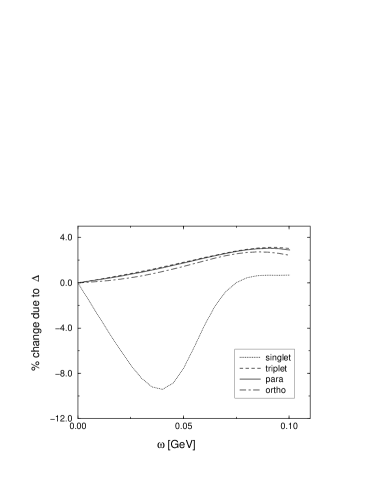
FIG. 5.: Relative change in the photon spectra for RMC due to explicit $\Delta$(1232) related effects for the singlet, triplet, para (statistical) and ortho states of the $\mu-p$ system.

 

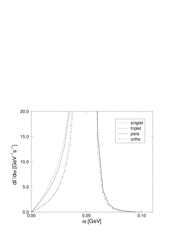
FIG. 6.: ${\cal O}(p^{2})$ HBChPT photon spectra for RMC for the singlet, triplet, para (statistical) and ortho states of the $\mu-p$ system in the chiral limit.

FIG. 7.: The “world data” for the induced pseudoscalar form factor $G_{P}(t)$. Dashed curve: Pion–pole prediction. Solid curve: ${\cal O}(\epsilon^{3})/{\cal O}(p^{3})$ SSE/HBChPT prediction. The pion electroproduction data (crosses) are from ref.[8]. Also shown is the OMC result at $t=-0.88m_{\mu}^{2}$ from ref.[7] (open square).

FIG. 8.: Photon spectra for RMC for the branching ratios of the singlet, ortho and para states as used in the TRIUMF analysis. Solid line: Prediction of the small scale expansion to order $\epsilon^{2}$. Dash–dotted line: Same as the solid line but with $g_{P}$ scaled by a factor $1.5$. Dashed line: Various small modifications as explained in the text. Dotted line: Same as the dashed line but using the neutral instead of the charged pion mass.

REFERENCES

- [1] J. Govaerts and J.-L. Lucio-Martinez, [nucl-th/0004056]
- [2] S.L. Adler and Y. Dothan, Phys. Rev. 151 (166) 1267.
- [3] L. Wolfenstein, in “High-Energy Physics and Nuclear Structure”, ed. by S. Devons (Plenum, New York, 1970) p. 661.
- [4] V. Bernard, N. Kaiser and Ulf-G. Meißner, Phys. Rev. D50 (1994) 6899.
- [5] V. Bernard, H.W. Fearing, T.R. Hemmert and Ulf-G. Meißner, Nucl. Phys. A635 (1998) 121.
- [6] H.W. Fearing, R. Lewis, N. Mobed and S. Scherer, Phys. Rev. D56 (1997) 1783.
- [7] G. Bardin et al., Phys. Lett. B104 (1981) 320.
- [8] S. Choi et al., Phys. Rev. Lett. 71 (1993) 3927.
-
[9]
G. Jonkmans et al., Phys. Rev. Lett. 77 (1996) 4512;
D.H. Wright et al., Phys. Rev. C57 (1998) 373. - [10] D. Beder and H.W. Fearing, Phys. Rev. D39 (1989) 3493.
- [11] G.I. Opat, Phys. Rev. 134 (1964) B428.
- [12] D. Beder, Nucl. Phys. A258 (1976) 447.
- [13] H.W. Fearing, Phys. Rev. C21 (1980) 1951.
- [14] D. Beder and H.W. Fearing, Phys. Rev. D35 (1987) 2130.
- [15] T. Meissner, F. Myhrer and K. Kubodera, Phys. Lett. B416 (1998) 36.
- [16] S.-I. Ando and D.-P. Min, Phys. Lett. B417 (1998) 177.
- [17] I.-T. Cheon and M.K. Cheoun, [nucl-th/9811009].
- [18] J. Smejkal and E. Truhlik, [nucl-th/9811080].
- [19] T.R. Hemmert, B.R. Holstein and J. Kambor, Phys. Lett. B395, 89 (1997).
- [20] T.R. Hemmert, B.R. Holstein and J. Kambor, J. Phys. G24, 1831 (1998).
- [21] e.g. N.C. Mukhopadhyay,[nucl-th/9810039].
- [22] J. Smejkal, E. Truhlik and F.C. Khanna, Few Body Syst. 26, 175 (1999).
- [23] V. Bernard, T.R. Hemmert and Ulf-G. Meißner in “Baryons’98”, D.W. Menze and B. Ch. Metsch (eds.) (World Scientific, Singapore, 1999).
- [24] J. Gasser and H. Leutwyler, Ann. Phys. (NY) 158 (1984) 142.
- [25] A.V. Manohar and E. Jenkins, Phys. Lett. B255 (1991) 353; ibid B259 (1991) 353.
- [26] V. Bernard, N. Kaiser, J. Kambor and Ulf-G. Meißner, Nucl. Phys. B388 (1992) 315.
- [27] V. Bernard, N. Kaiser and Ulf-G. Meißner, Int. J. Mod. Phys. E4 (1995) 193.
-
[28]
W.R. Wessel and P. Phillipson, Phys. Rev. Lett. 13, 23
(1964);
D.D. Bakalov, M.P. Faifman, L.I. Ponomarev and S.I. Vinitsky, Nucl. Phys. A384, 302 (1982). - [29] G.G. Petratos, Nucl. Phys. A666&667, 61c (2000); Ulf-G. Meißner, Nucl. Phys. A666&667, 51c (2000).
- [30] H. Primakoff, Rev. Mod. Phys. 31 (1959) 802.
- [31] A. Santisteban and R. Pascual, Nucl. Phys. A260, 392 (1960).
- [32] S. Weinberg, Phys. Rev. Lett. 4, 575 (1960).
- [33] e.g. D.D. Bakalov and S.I. Vinitsky, Sov. J. Nucl. Phys. 32, 372 (1980) and references therein.
- [34] D.V. Balin et al., PSI-proposal R-97-05.1.
- [35] P. Bartsch et al. (A1 Collaboration), MAMI-proposal A1/1-98.
- [36] G.C. Gellas, T.R. Hemmert, C.N. Ktorides and G.I. Poulis, Phys. Rev. D60, 054022 (1999).
- [37] S.-I. Ando, F. Myhrer and K. Kubodera, [nucl-th/0008003].