Particle Multiplicities and Thermalization in High Energy Collisions

Abstract

We investigate the conditions under which particle multiplicities in high energy collisions are Boltzmann distributed, as is the case for hadron production in $e^{+}e^{-}$, $pp$, $p\bar{p}$ and heavy ion collisions. We show that the apparent temperature governing this distribution does not necessarily imply equilibrium (thermal or chemical) in the usual sense, as we explain. We discuss an explicit example using tree level amplitudes for $N$ photon production in which a Boltzmann-like distribution is obtained without any equilibration. We argue that the failure of statistical techniques based on free particle ensembles may provide a signal for collective phenomena (such as large shifts in masses and widths of resonances) related to the QCD phase transition.

1 Introduction

The use of thermal or statistical models to describe multiparticle production has a long history [1]. Recent studies [References–References] observe that the multiplicities of hadron production in a variety of contexts ($e^{+}e^{-}$, $pp$, $p\bar{p}$ and heavy ion collisions) are extremely well described by models involving thermal distributions of free hadrons. The only free parameters in their analysis are the temperature and volume of the model thermal system, and a parameter reflecting the level of equilibration of strange particles (in the heavy ion case the baryon chemical potential is an additional parameter). One might conclude from their results that thermal and chemical equilibrium among hadrons is already reached in individual jets produced in high-energy scattering.

However, this conclusion is somewhat unjustified, given that any mechanism for producing hadrons which evenly populates the free particle phase space will mimic a microcanonical ensemble, and therefore yield apparently thermal results. It is important to remark that this type of apparent thermalization will always yield Boltzmann weights which are functions of the free particle energy, and hence describe a non-interacting ensemble. True QCD thermalization, of the type associated with the quark-gluon plasma (QGP), and that experimentalists hope to observe at RHIC, involves large collective effects, and hence is probably poorly modelled by a non-interacting hadron gas.

Here we address the problem of deducing whether a process which leads to multiparticle production is thermal. We make the important distinction between phase space dominated phenomena, which lead to ensembles governed by free particle Boltzmann weights, and interacting thermal ensembles, in which collective effects can be important. We argue that a process which generates data that can be fit using free particle ensembles is merely good at populating phase space in a uniform way – it has not necessarily produced an interacting thermal region. In QCD, a region of this type with temperature of order 100 MeV or more should exhibit strong collective phenomena, such as hadron mass shifts, that preclude description in terms of a free particle ensemble. Hence, we argue that the failure of statistical techniques based on free particle ensembles should be regarded as a signal for the onset of true equilibration at heavy ion colliders such as RHIC.

This paper is organized as follows. In section 2 we review the relation between microcanonical and canonical ensembles in statistical mechanics. We argue that multiparticle production in many cases is equivalent to a method of populating a modified microcanonical ensemble. Such an ensemble will produce “thermal” behavior even if there is no subsequent interaction of particles once produced. In section 3 we apply our results to multiparticle production and examine a specific example in a toy model involving tree-level photon production. In this toy model there is clearly no real thermal equilibrium – once produced, the photons do not interact. However, a quasi-Boltzmann distribution results in the limit where a large number of photons is produced. In section 4 we discuss the implications of our conclusions for heavy ion collisions.

2 Microcanonical vs Canonical Ensembles

Here we give a brief review of the relationship between the microcanonical and canonical ensembles (MCE and CE, respectively) in statistical mechanics. Recall that the MCE sums only over states with some fixed total energy, while the CE sums over all states with Boltzmann weight $e^{-\beta E}$. The main result is rather familiar: under certain general assumptions, quantities computed in the MCE differ from those computed in the CE by an amount which vanishes as the size of the system $N$ is taken to infinity. The importance of this result is as follows: the cross section for particle production in a high energy collision can be written as the expectation of the matrix element squared in the MCE corresponding to the free theory. In the limit of large $N$, one can therefore rewrite the usual phase space integral appearing in a cross section in terms of the average of the matrix element squared in a CE, which is controlled by the Boltzmann factor. This naturally leads to a certain “thermal” behavior which we discuss below.

In the MCE the total energy is fixed and the probability density is constant over all of phase space. The computation of the entropy $S(E)$ is as follows:

$$\Gamma(E)=\sum_{s}\delta(E_{s}-E),$$ (1)

$$S(E)=\ln\Gamma(E).$$ (2)

In Eq. (1), $E_{s}$ is the energy of the state $s$. It is often more convenient to replace the delta function in (1) with the factor $\Delta(E)\equiv\exp(-\beta(E_{s}-E))$, yielding a new quantity, the CE:

$$\bar{\Gamma}(E)=\sum_{s}e^{-\beta(E_{s}-E)}.$$ (3)

In the canonical ensemble there is no restriction on the energies of the states $s$. However, they appear with Boltzmann weight $\exp(-\beta E_{s})$. The new quantity introduced, $\beta$, describes the temperature of the system, which is fine-tuned to ensure that the average energy is $E$. To see this, rewrite $\bar{\Gamma}(E)$ as follows:

$$\bar{\Gamma}(E) = \int dE^{\prime}~{}\sum_{s}e^{-\beta(E^{\prime}-E)}\delta(E_{s}-E^{\prime})$$ (4)

$$= \int dE^{\prime}~{}\Gamma(E^{\prime})~{}e^{-\beta(E^{\prime}-E)}$$

$$= \int dE^{\prime}~{}e^{S(E^{\prime})-\beta(E^{\prime}-E)}.$$

Now evaluate (4) in the saddle-point approximation. (This is also known as the Darwin-Fowler method [13].) Let

$$\beta~{}=~{}{\partial S\over\partial E^{\prime}}\Bigg{|}_{E}~{}~{},$$ (5)

so

$$\bar{\Gamma} = e^{S(E)}~{}\int dE^{\prime}~{}e^{\frac{1}{2}S^{\prime\prime}(E)(E^{\prime}-E)^{2}+\cdots}$$ (6)

$$= \sqrt{2\pi\over-S^{\prime\prime}(E)}~{}e^{S(E)}~{}+~{}\cdots~{}~{}~{}.$$

Here we have assumed that $S^{\prime}(E)>0$ (positive temperature) and $S^{\prime\prime}(E)<0$ (positive specific heat). It is easy to see that the difference between the CE entropy $\bar{S}(E)=\ln\bar{\Gamma}(E)$ and the MCE entropy $S(E)$ is of order $(\ln N)/N$. The terms represented by the ellipsis in (6) lead to even smaller corrections, and will be neglected.

Now consider a generic operator ${\cal O}$. The average in the CE is given by

$$\langle{\cal O}\rangle_{C} = {1\over\bar{\Gamma}(E)}\sum_{s}e^{-\beta(E_{s}-E)}~{}{\cal O}_{s}$$ (7)

$$= e^{-S(E)}\sqrt{-S^{\prime\prime}(E)\over 2\pi}~{}\int dE^{\prime}~{}e^{S(E^{\prime})-\beta(E^{\prime}-E)}\thinspace\thinspace\langle{\cal O}\rangle_{M}(E^{\prime}),$$

where $\langle{\cal O}\rangle_{M}$ is the average taken in the microcanonical ensemble. Its logarithm can be expanded as follows

$$\ln[\langle{\cal O}\rangle_{M}(E^{\prime})]=\ln[\langle{\cal O}\rangle_{M}(E)]~{}+~{}(E^{\prime}-E)\ln^{\prime}[\langle{\cal O}\rangle_{M}(E)]~{}+~{}\frac{1}{2}(E^{\prime}-E)^{2}\ln^{\prime\prime}[\langle{\cal O}\rangle_{M}(E)]~{}+~{}\cdots.$$ (8)

The integral in (7) can again be performed in the saddle-point approximation. Note that if the operator ${\cal O}$ is of order $N$ (as in the case of a particle multiplicity), the coefficients appearing in the expansion (8) are of order $\ln N$. They lead to small shifts (of order $(\ln N)/N$) in the saddle-point value of the temperature $\beta$ and the overall prefactor. Thus the canonical and microcanonical averages of particle multiplicities converge in the limit of large $N$.

In the next section we apply these results to the computation of cross sections for particle production in high energy collisions.

3 Multiplicity Results

The cross section for the process $A+B\rightarrow n$ particles is

$$\sigma={1\over 2E_{A}2E_{B}|v_{A}-v_{B}|}\int\prod_{f}{d^{3}p_{f}\over(2\pi)^{3}}{1\over 2E_{f}}~{}|{\cal M}|^{2}~{}(2\pi)^{4}\delta^{(4)}\biggl{(}p_{A}+p_{B}-\sum_{f}p_{f}\biggr{)}.$$ (9)

First, let us assume that the function $|{\cal M}|^{2}/\prod 2E_{f}$ in the dominant region of phase space is slowly varying (we will relax this assumption shortly). Then, we can use the following approximation

$$\sigma={1\over 2E_{A}2E_{B}|v_{A}-v_{B}|}~{}{|\bar{\cal M}|^{2}\over\prod_{f}2\bar{E}_{f}}\int\prod_{f}{d^{3}p_{f}\over(2\pi)^{3}}~{}(2\pi)^{4}\delta^{(4)}\biggl{(}p_{A}+p_{B}-\sum_{f}p_{f}\biggr{)},$$ (10)

where $\bar{\cal M},\bar{E}$ are averaged quantities. As noted, the integral in (10) is just the microcanonical ensemble for $N$ free particles, and hence leads to “thermal” properties of the particle distributions and multiplicities. Considering the more general case where the number of particles is not fixed, we simply sum over all cross sections,

$$\sigma=\sum_{n}\sigma_{AB\rightarrow n},$$ (11)

to obtain a MCE without fixed particle number. In the usual thermodynamic limit this sum is dominated by some particular value of $n$, so it is equivalent to consider the earlier case with $n=N$.

We now treat the matrix element more carefully, by retaining it in the phase space integral. The resulting integral can still be turned into a canonical ensemble using the result of the previous section, provided the modified “entropy” (i.e., the logarithm of the phase space integral including the matrix element) continues to grow with total energy $E$ (positive temperature), and the second derivative of this entropy with respect to $E$ is negative (positive specific heat). The energy-momentum delta function can then be replaced by a Boltzmann weight $\exp[(p_{A}{+}p_{B}{-}\sum p_{f})\cdot\beta]$, which in the center of mass frame reduces to $\exp[\beta(E{-}\sum E_{f})]$. This yields the following result for the differential cross section:

$${d^{3}\sigma\over dp^{3}_{i}}\propto{1\over E_{i}}\thinspace e^{-E_{i}/T}\int\prod_{f\neq i}d^{3}p_{f}\thinspace{1\over E_{f}}~{}|{\cal M}|^{2}~{}\exp\left({-\sum_{f\neq i}E_{f}/T}\right).$$ (12)

Note the natural appearance of the Boltzmann factor in (12).

To proceed further, we need a specific model for the behavior of the matrix element. There are very few cases in which the matrix element for $N$-particle production is explicitly known. One such case is the QED process

$$f\bar{f}\rightarrow 1\enspace\hbox{spin up photon}+(n-1)\enspace\hbox{spin down photons},$$ (13)

where the (massless) fermions have opposite spin. The matrix element squared for (13) is [14]

$$|{\cal M}(P_{\uparrow},Q_{\downarrow};1_{\uparrow},2_{\downarrow},\cdots,n_{\downarrow})|^{2}=(2e^{2})^{n}\thinspace\thinspace{{(2Q\cdot p_{1})^{2}}\over{(2P\cdot Q)}}\thinspace\prod^{n}_{i=2}{{(2P\cdot Q)}\over{(2P\cdot p_{i})(2p_{i}\cdot Q)}},$$ (14)

where $P$, $Q$ and $p_{i}$ are the momenta of the two incoming fermions and $n$ outgoing gauge particles respectively. In the $(P,Q)$ center of momentum frame this may be written as

$$|{\cal M}(P_{\uparrow},Q_{\downarrow};1_{\uparrow},2_{\downarrow},\cdots,n_{\downarrow})|^{2}={\cal K}E_{1}^{2}(1+\cos\theta_{1})^{2}\prod^{n}_{i=2}{{1}\over{E^{2}_{i}\sin^{2}\theta_{i}}},$$ (15)

where $E_{i},\theta_{i}$ are the energy and production angle of the $i$th photon, and we have lumped all of the remaining constant factors into ${\cal K}$. Using this to solve for the differential cross section yields ($i\neq 1$)

$$d^{3}\sigma\propto{{1}\over{E^{3}_{i}\sin^{2}\theta}}\thinspace e^{-E_{i}/T}\thinspace d^{3}p_{i}.$$ (16)

The resulting number density of (spin down) photons is then

$$n\propto\int{d^{3}p\over(2\pi)^{3}}~{}{1\over E^{3}~{}\sin^{2}\theta}~{}e^{-E/T}.$$ (17)

In this particular example we have a problem, because the photons are massless and there is an infrared catastrophe due to arbitrarily soft photons. Of course, the number density of observable photons – those with some minimum energy and angular separation from the initial $f\bar{f}$ pair – is finite. For our purposes, we can always eliminate this problem by introducing a photon mass by hand in our toy model. In fact, we can introduce several species of “photons” with masses $m_{i}$. Then, the abundance of each species is given by

$$n_{i}~{}\propto~{}\int{d^{3}p\over(2\pi)^{3}}~{}{1\over(p^{2}+m_{i}^{2})^{3/2}}~{}e^{-\sqrt{p^{2}+m_{i}^{2}}/T}.$$ (18)

The integral in (18) differs from the one appearing in a pure Boltzmann distribution due to the factor of $(p^{2}+m_{i}^{2})^{-3/2}$. Without this extra factor, the integral simply reduces to $m_{i}^{2}TK_{2}(m_{i}/T)$, where $K_{2}(x)$ denotes the modified Bessel function of order 2.

In a sense, the additional factor makes only a small difference relative to the exponential: when taken into the exponent it is of order $\ln(\beta E)$, versus $\beta E$ for the Boltzmann factor. However, actual ratios of particle abundances $n_{i}/n_{j}$ will differ from thermal ratios. In Fig. 1 we show the result of the multiplicities from (18) and a thermal best fit. While we didn’t use any additional parameters, such as individual chemical potentials, the eventual quality of the fit would probably not be as good as what is observed in $e^{+}e^{-}$, $pp$, $p\bar{p}$ and heavy ion collisions [References–References]. In other words, the hadronization process probably populates free particle phase space somewhat more evenly than our toy model. However, our toy model does demonstrate that Boltzmann-like distributions are not necessarily indicative of real thermal (chemical or kinetic) equilibrium.

Figure 1: Multiplicity vs. particle species mass of the toy-model, and thermal fit.

4 Discussion

In the previous sections we argued that multiparticle production can readily lead to thermal behavior if the the process in question is phase space dominated. Because phase space is determined by free particle kinematics, the results correspond to an ensemble of non-interacting particles. In other words, because the arguments of the energy delta function in the cross section Eq. (9) are simply free particle energies, the corresponding Hamiltonian appearing in the ensemble in Eqs. (1) and (3) is the free Hamiltonian, with no interactions. Our toy model of photons suggests that this result is rather generic in any process where a large number of particles is produced.

If the ensemble is dominated by a particular species of particle (i.e. the lightest particle), the apparent “temperature” will be related to the mass $m$ of that species. This is because phase space is maximized by producing as many particles as possible, each with a kinetic energy of order $m$. Suspiciously, the typical temperatures produced by the excellent thermal fits of $e^{+}e^{-}$, $pp$, $p\bar{p}$ and heavy ion collisions [References–References] are all of order the pion mass.

Of course, an ensemble of non-interacting hadrons is not very interesting. It gives us no information about the actual QCD phase diagram. In real QCD the energy of a state consisting of many particles is modified due to interactions: it is not simply the sum of the free particle energies. At high density or temperature interaction effects are large and lead to large deviations from free particle results. Were this not so one could never see collective phenomena such as chiral symmetry restoration or a deconfinement phase transition. In an ensemble of interacting hadrons we already expect significant collective effects at temperatures $T\sim m_{\pi}$, such as a decrease in the value of the quark condensate $\langle\bar{q}q\rangle_{T}$, and shifts in the various hadron masses.

We expect these effects to lead to the failure of statistical techniques based on free particle ensembles, which predict that the multiplicities should fall roughly exponentially (as $e^{-m/T}$, see Fig. 1). However, if the masses and widths are shifted from their vacuum values at the instant of chemical freeze-out, as would be expected at the $\sim 170$ MeV temperatures obtained in the fits, then a plot of multiplicity versus vacuum mass will deviate from the thermal prediction: i.e. it will have the form $e^{-m(T)/T}$. On the other hand, it is also possible that the system will remain in equilibrium long enough for the masses and widths to return to their vacuum values. If so, then a thermal fit will perform well, but the resulting temperature would not be near the chiral phase transition.

Knowledge of these mass shifts would be necessary for any detailed predictions. Although there have been some promising results [15], it has proven difficult to extract this information from lattice data. A perturbative estimate of the decrease in the quark condensate was derived in Ref. [16]. In the chiral limit ($m_{u}=m_{d}=0$), an analytic result is possible. It reads

$$\langle\bar{q}q\rangle_{T}~{}=~{}\langle\bar{q}q\rangle_{T=0}\Biggl{[}1-{3T^{2}\over 24F^{2}}-\frac{3}{8}\Biggl{(}{T^{2}\over 12F^{2}}\Biggr{)}^{2}+{\cal O}(T^{6})\Biggr{]},$$ (19)

where $F\approx 93$ MeV is the (zero temperature) pion decay constant. Using real world quark masses changes this result only slightly. The corresponding estimate for the temperature of the chiral phase transition (i.e. the point at which the condensate is essentially zero) is 170 MeV in the chiral limit, and 190 MeV in the real world, consistent with lattice data.

We expect the thermal pion mass to obey the finite temperature version of the Dashen formula

$$m^{2}_{\pi}(T)~{}\simeq~{}{2m_{q}\over F^{2}(T)}\thinspace|\langle\bar{q}q\rangle_{T}|,$$ (20)

where (again, for two massless flavors) [16]

$$F^{2}(T)~{}=~{}F^{2}(0)\Biggl{[}1-{T^{2}\over 6F^{2}(0)}+{\cal O}(T^{4})\Biggr{]}.$$ (21)

Note that at leading order the thermal pion mass actually increases slightly with temperature. The temperature dependence of the baryon masses is a harder problem, but in the naïve quark model we might expect them to behave roughly as

$$m_{B}(T)~{}\simeq~{}3~{}|\langle\bar{q}q\rangle_{T}|,$$ (22)

where the constituent quark mass is simply due to the condensate. This estimate at least incorparates the fact that the baryons must become nearly massless at the chiral phase boundary, since chiral symmetry prevents them from obtaining a mass. Equations (20) and (22) suggest that the relative abundance of baryons compared to pions will increase at high temperature. While we don’t necessarily believe that (22) is very accurate, the point is that the thermal pion and baryon masses probably do not depend on the quark condensate (and hence the temperature) in the same way. Thus, it is probably inconsistent to imagine fitting the properties of an interacting hadron gas at $T\sim m_{\pi}$ using vacuum hadron masses. Yet, essentially all recent heavy ion data agrees well with multiplicities generated by free thermal models, with temperatures of roughly $T\sim 50-170$ MeV.

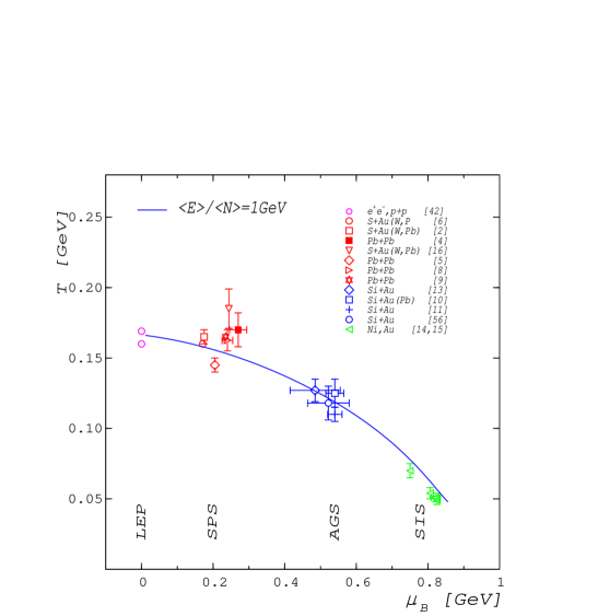
Figure 2: Temperatures and chemical potentials obtained by Cleymans and Redlich [12] from thermal multiplicity fits of LEP, CERN/SPS, BNL/AGS and GSI/SIS data.

In Fig. 2 we reproduce a plot from the paper of Cleymans and Redlich [12], where the fitted temperatures and chemical potentials resulting from LEP, CERN/SPS, BNL/AGS and GSI/SIS data are displayed. One interpretation of these results (which we do not subscribe to) is that a large region of the QCD phase diagram in the temperature-density plane has already been explored! There is no question that the quality of the free thermal fits is quite good. However, this in itself suggests that an interacting thermal region has yet to be produced in these experiments. Rather, it is quite possible that the collisions simply serve as a mechanism for populating phase space, without ever evolving through configurations in real thermal and chemical equilibrium (i.e. actual points on the phase diagram in Fig. 2). If the system had passed through real equilibrium, we suggest that the observed final state multiplicities could deviate significantly from those which can be generated by free thermal models. Thus the failure of such models to fit the data could be a signal for real equilibrium. This idea is explored in the context of phenomenologically motivated models in [17]. For more recent work related to this paper, which originally appeared as preprint nucl-th/0001044 in 2000, see [18].

References

- [1] E. Fermi, Prog. Theor. Phys. 5, 570 (1950); L.D. Landau, Izv.Akad.Nauk Ser. Fiz. 17, 51 (1953); R. Hagedorn, Nuovo Cimento Suppl. 3, 147 (1965).
- [2] For a review, see, e.g., U. Heinz, J. Phys. G25, 263 (1999); talk presented at the 14th International Conference on Ultrarelativistic Nucleus-Nucleus Collisions, Torino, Italy, May 1999, nucl-th/9907060.
- [3] F. Becattini, Z. Phys. C69, 485 (1996).
- [4] F. Becattini, Firenze Preprint DFF 263/12/1996, hep-ph/9701275.
- [5] F. Becattini and U. Heinz, Z. Phys. C76, 269 (1997).
- [6] J. Sollfrank, M. Gazdzicki, U. Heinz and J. Rafelski, Z. Phys. C61, 659 (1994).
- [7] P. Braun-Munzinger, J. Stachel, J.P. Wessels and N. Xu, Phys. Lett. B365, 1 (1996).
- [8] P. Braun-Munzinger and J. Stachel, Nucl. Phys. A606, 320 (1996).
- [9] F. Becattini, M. Gaździcki and J. Sollfrank, Nucl. Phys. A638, 403 (1998); Eur. Phys. J. C5, 143 (1998).
- [10] J. Sollfrank, Eur. Phys. J. C9, 159 (1999).
- [11] P. Braun-Munzinger, I. Heppe and J. Stachel, Phys. Lett. B465, 15 (1999).
- [12] J. Cleymans and K. Redlich, Phys. Rev. C60, 054908 (1999).
- [13] T.T. Chou, C.N. Yang and E. Yen, Phys.Rev.Lett. 54, 510 (1985);T.T. Chou and C.N. Yang, Phys.Rev.Lett. 55, 1359 (1985).
- [14] S.J. Parke and T.R. Taylor, Phys. Rev. Lett. 56, 2459 (1986); G. Mahlon and T.–M. Yan, Phys. Rev. D47, 1776 (1993).
- [15] Y. Nakahara, M. Asakawa, and T. Hatsuda, talk given at the 17th International Symposium on Lattice Field Theory (LATTICE 99), Pisa, Italy, hep-lat/9909137.
- [16] J. Gasser and H. Leutwyler, Phys. Lett. B184, 83 (1987); P. Gerber and H. Leutwyler, Nucl. Phys. B321, 387 (1989).
- [17] S. Pratt and K. Haglin, Phys. Rev. C59, 3304 (1999).
- [18] D. Rischke, NPA 698, 153C (2002); V. Koch nucl-th/0210070; U. Heinz, nucl-th/0212004; J. Rafelski, nucl-th/0212091.