Dissipative dynamics of fission in the framework of asymptotic expansion of Fokker-Planck equation

Abstract

The dynamics of fission has been formulated by generalising the asymptotic expansion of the Fokker-Planck equation in terms of the strength of the fluctuations where the diffusion coefficients depend on the stochastic variables explicitly. The prescission neutron multiplicities and mean kinetic energies of the evaporated neutrons have been calculated and compared with the respective experimental data over a wide range of excitation energy and compound nuclear mass. The mean and the variance of the total kinetic energies of the fission fragments have been calculated and compared with the experimental values.

I introduction

At present, it is commonly agreed upon that the fission process is a dissipative phenomena, where initial energy of the collective variables get dissipated into the internal degrees of freedom of nuclear fluid giving rise to the increase in internal excitation energy. As dissipation is referred to the interaction of the system coordinate with the large number of degrees of freedom of the surrounding reservoir, this process is always associated with the fluctuations of relevant physical observables. Thus, the dynamics of fission process resembles the standard Brownian motion problem, where the collective variables such as shape degrees of freedom act as ’Brownian particles’ interacting stochastically with large number of internal nucleonic degrees of freedom constituting the surrounding ’bath’. This mesoscopic description is inevitable once the fluctuations of the observables are amenable to experimental observation.

There have been several attempts in the past to study the dynamics of fission by solving either the Langevin equation [1, 2, 3, 4], or multidimensional Fokker-Planck equation [5, 6, 7, 8], which is a differential version of Langevin equation. In the case of fission, it is experimentally observed that the variances of the physical observables are, in general, small compared to their respective mean values ( typically, the ratio of the root mean square deviation and the mean of the kinetic energy is $\sim$ 0.1). The question naturally arises whether one can utilise this simple fact in the theoretical scheme instead of solving the Langevin equation (LE) or corresponding Fokker-Planck equation in detail. In this spirit, we present an alternative theoretical prescription for the calculation of various moments of the physical observables related to the fission process based on the assumption that the full solution of the Fokker-Planck equation (FPE) admits an asymptotic expansion in terms of strength of the fluctuations. The asymptotic expansion method was first developed by van Kampen [9] for the stochastic processes having constant diffusion coefficients. However, a generalisation of the above prescription is necessary in the case of fission where the dissipation is usually assumed to depend on the instantaneous shape of the fissioning system and therefore the diffusion coefficients are also shape dependent. To the best of our knowledge, such an application in the case of fission is not available in the literature.

In the present paper, we report a generalised formulation of the asymptotic expansion of the Fokker-Planck equation where the diffusion coefficient depends on the stochastic variables explicitly. In this formulation the dynamics of the stochastic processes reduces to a set of linear ordinary differential equations which are far simpler to solve as compared to either multidimensional partial differential ( Fokker-Planck) equations or stochastic differential (Langevin) equations. Presently, we apply this formulation to calculate the various moments of the relevent physical observables of the fission process.

The paper is organised as follows.The generalised formulation and its application to the dynamics of fission is given in Sec. II. The calculations and numerical results are discussed in Sec.III. Finally, concluding remarks are given in Sec.IV.

II Asymptotic expansion of the Fokker-Planck equation

A The Formalism

The mesoscopic description of the fission process begins with a set of Langevin equations:

$$\dot{X_{i}} = h_{i}(\{X\},\{Y\})+\eta_{i}(t)$$ (2)

$$\dot{Y_{i}} = H_{i}(\{X\},\{Y\})\hskip 18.0pt;i=1,...,N$$ (3)

where $h_{i}$ and $H_{i}$ are given functions of the stochastic collective variables $X_{1},X_{2},...,X_{N}$ and $Y_{1},Y_{2},...,Y_{N}$ in the fission process and $\eta_{i}(t)$ refers to the driving noise term associated with the interaction of the ith collective variable with the reservoir constituting nucleonic degrees of freedom. For simplicity, we assume the noise to be a gaussian white with zero mean and decoupled for different degrees of freedom with auto-correlation functions given by

$$<\eta_{i}(t)>=0,\hskip 8.0pt<\eta_{i}(t)\eta_{j}(t^{\prime})>=D_{i}(y_{i})\delta(t-t^{\prime})\delta_{ij},$$ (4)

where $D_{i}(y_{i})$ is the diffusion coefficient associated with ith variable, depending only on the sample space $y_{i}$ for the stochastic variable $Y_{i}$.

The Fokker-Planck equation corresponding to the Langevin equation (2.1) is

$$\frac{\partial f(\{x\},\{y\},t)}{\partial t}=-\sum_{i}[\frac{\partial(h_{i}f)}{\partial x_{i}}+\frac{\partial(H_{i}f)}{\partial y_{i}}-(1/2)D_{i}(y_{i})\frac{\partial^{2}f}{\partial x_{i}^{2}}].$$ (5)

The quantity $f(\{x\},\{y\},t)$ is the probability density function depending on the variables $x_{1},x_{2},...,x_{N},y_{1},y_{2},...,y_{N}$ and time $t$ explicitly. If we are interested in finding the time evolution of the conditional probability distribution function then we have to solve Eq.(2.3) with initial values $x_{i}(0)=x_{i}^{0}$, $y_{i}(0)=y_{i}^{0}$, $\forall$$i$, at $t=0$. That is, we have to solve Eq.(2.3) for those realisations which are known to start from these specific points in the whole sample space.

In the cases where diffusion coefficient is constant the asymptotic expansion method of van Kampen [9] consists of writing the stochastic variables as the sum of deterministic value and a fluctuating part at each time $t$ with root of the diffusion constant as a strength of the fluctuating part. In the present paper, we generalise this method for the situations where the diffusion coefficients depend on the stochastic variables explicitly. Such a situation is encountered in the case of fission process, where the friction coefficient depends explicitly on the collective variable or shape of the nucleus at each instant of time. In this case, we further assume that, in the asymptotic expansion, the strengths of the fluctuating parts of the stochastic variables depend only on the deterministic values of the respective $y$ variables:

$$x_{i} = \bar{x_{i}}+\surd D(\bar{y_{i}})\zeta_{i}$$ (7)

$$y_{i} = \bar{y_{i}}+\surd D(\bar{y_{i}})\xi_{i}$$ (8)

The quantities $\{\zeta_{i}\},\{\xi_{i}\}$ refer to the fluctuations of the stochastic variables $\{x_{i}\}$ and $\{y_{i}\}$ around their deterministic values $\{\bar{x_{i}}\},\{\bar{y_{i}}\}$. Next, we introduce the new distribution function $Q$ depending only on the variables $\{\zeta_{i}\}$,$\{\xi_{i}\}$ and $t$. The normalisation condition suggests that the $f$ and $Q$ will be related by

$$f(\{x\},\{y\},t)={\prod_{i=1}^{N}[D_{i}(\bar{y_{i}})]^{-1}}Q_{i}(\zeta_{i},\xi_{i},t)$$ (9)

Substituting Eq.(2.4) in the Fokker-Planck equation(2.3), making Taylor expansion of $h(\{x\},\{y\}),H(\{x\},\{y\})$ around $\{\bar{x}\},\{\bar{y}\}$ and collecting coefficients of various order of $D(\bar{y_{i}})$,we could generate a hierarchy of equations. As expected, the first set would give rise to the equation of motion for $\{\bar{x}\}$ and $\{\bar{y}\}$.

$$\dot{\bar{x_{i}}} = h_{i}(\{\bar{x}\},\{\bar{y}\})$$ (11)

$$\dot{\bar{y_{i}}} = H_{i}(\{\bar{x}\},\{\bar{y}\})\hskip 18.0pt;\forall{i}$$ (12)

Eqs.(2.6) are the Euler-Lagrange equation for deterministic motion. These equations are to be solved with initial conditions $\{\bar{x}(0)\}=\{x^{0}\},\{\bar{y}(0)\}=\{y^{0}\}$. Next, we are going to calculate the conditional probability distribution $f(\{x\},\{y\},t\mid\{x^{0}\},\{y^{0}\},0)$ or $Q(\{\zeta\},\{\xi\},t\mid 0,0,0)$.

Assuming the variation of diffusion coefficient over the narrow width of the distribution function at any instant of time to be $\bigcirc(D)$, we could replace the second Fokker-Planck coefficient $D(y)$ by $D(\bar{y})$ at each instant of time. This assumption makes the calculation extremely simple. Collecting coefficients $\bigcirc(D^{0})$, we get back quasilinear Fokker-Planck equation for $Q$:

$$\frac{\partial Q}{\partial t}+\sum_{i}(\frac{\dot{D}(\bar{y}_{i})}{D(\bar{y}_{i})})Q=-\sum_{i}[a_{i}\frac{\partial(\zeta_{i}Q)}{\partial\zeta_{i}}+b_{i}\frac{\partial(\xi_{i}Q)}{\partial\zeta_{i}}+c_{i}\frac{\partial(\xi_{i}Q)}{\partial\xi_{i}}+d_{i}\frac{\partial(\zeta_{i}Q)}{\partial\xi_{i}}-(1/2)\frac{\partial^{2}Q}{\partial\zeta_{i}^{2}}]$$ (13)

where $a_{i},b_{i},c_{i},d_{i}$ are given by

$$a_{i} = (\frac{\partial h}{\partial\bar{x}_{i}})-(\frac{\dot{D}(\bar{y}_{i})}{2D(\bar{y}_{i})})$$ (15)

$$b_{i} = (\frac{\partial h}{\partial\bar{y}_{i}})$$ (16)

$$c_{i} = (\frac{\partial H}{\partial\bar{y}_{i}})-(\frac{\dot{D}(\bar{y}_{i})}{2D(\bar{y}_{i})})$$ (17)

$$d_{i} = (\frac{\partial H}{\partial\bar{x}_{i}})$$ (18)

Eq.(2.7) suggests that

$$Q(\{\zeta\},\{\xi\},t)=\prod_{j}Q_{j}(\zeta_{j},\xi_{j},t)$$ (19)

where the distribution function $Q_{j}$ for each $j$ satisfies the similar equation written below without the subscript:

$$\frac{\partial Q}{\partial t}+(\frac{\dot{D}(\bar{y})}{D(\bar{y})})Q=-[a\frac{\partial(\zeta Q)}{\partial\zeta}+b\frac{\partial(\xi Q)}{\partial\zeta}+c\frac{\partial(\xi Q)}{\partial\xi}+d\frac{\partial(\zeta Q)}{\partial\xi}-(1/2)\frac{\partial^{2}Q}{\partial\zeta^{2}}]$$ (20)

subject to the initial condition

$$Q(\zeta,\xi,t=0)=\delta(\zeta)\delta(\xi)$$ (21)

The solution of Eq.(2.10) is given by

$$Q(\zeta,\xi,t)=[\frac{1}{(2\pi)^{2}}]\int\int exp-\{ik\zeta+il\xi+\frac{[g(t)k^{2}+G(t)l^{2}+2C(t)kl]}{2D(t)}\}dkdl$$ (22)

where $g(t),\ G(t),\ C(t)$ satisfy the set of coupled first order differential equations :

$$\frac{\dot{g}}{2} = (\frac{\partial h}{\partial x})g+(\frac{\partial h}{\partial y})C+\frac{D}{2}$$ (24)

$$\frac{\dot{G}}{2} = (\frac{\partial H}{\partial y})G+(\frac{\partial H}{\partial x})C$$ (25)

$$\dot{C} = (\frac{\partial h}{\partial x})C+(\frac{\partial h}{\partial y})G+(\frac{\partial H}{\partial y})C+(\frac{\partial H}{\partial x})g$$ (26)

with the initial conditions

$$g(0)=G(0)=C(0)=0$$ (27)

Once $Q(\zeta,\xi,t)$ is known, from Eq.(2.9) and Eq.(2.5) the full conditional probability distribution function $f(\{x\},\{y\},t\mid\{x^{0}\},\{y^{0}\},0)$ is known. Integrating this function over all variables except one, say $x_{i}$, one identifies $g_{i}(t)$ as the variance of the stochastic variable $X_{i}$.

$$<(X_{i}-<X_{i}>)^{2}>=g_{i}(t)$$ (28)

We note that the homogeniety of Eq.(2.10) suggests that $<\zeta(t)>=<\xi(t)>=0$, or the average of the variables $X$ and $Y$ at any time will be determined by their deterministic values obtained by solving Euler-Lagrange equation (2.6). Similarly, one observes from Eq.(2.12),

$$<(X_{i}-<X_{i}>)(Y_{i}-<Y_{i}>)> = C_{i}(t)$$ (30)

$$<(Y_{i}-<Y_{i}>)^{2}> = G_{i}(t)$$ (31)

B Application to the fission process

In the fission process, in accordance with our previous work [10], the shape of the fissioning nucleus is described in terms of the elongation axis (the neck parameter of [11] taken equal to zero). Thus, in the dynamical description we have the elongation axis, its relative orientation with respect to an inertial system and respective velocities associated with them as the stochastic variables interacting with a large number of internal nucleonic degrees of freedom constituting a heat bath at temperature $T$ determined by the excitation energy available to it. We further assume that the ’collisional’ time scale of the nucleonic degrees of freedom is much shorter than the time scale of the macroscopic evolution of the collective variable so that at each instant of time the heat bath is assumed to be in quasi-stationary equilibrium.

The Euler-Lagrange equations (2.6) were solved in our earlier works [10]. To avoid repetition we deliberately omit the procedure and scheme to solve those equations. For the sake of completeness we merely write those equations and refer to our previous papers to clarify the details.

Giving correspondence to the terminology used in this paper, we associate

$$Y_{1}=r,X_{1}=\dot{r},$$ (33)

$$Y_{2}=\theta,X_{2}=\dot{\theta}.$$ (34)

Thus we have

$$H_{1}(\{x,y\}) = x_{1}=\dot{r}$$ (36)

$$h_{1}(\{r,\dot{r}\}) = [\frac{L^{2}}{\mu r^{3}}-\gamma\dot{r}-\frac{\partial(V_{C}+V_{N})}{\partial r}]/\mu,$$ (37)

$$H_{2}(\{x,y\}) = x_{2}=\dot{\theta},$$ (38)

$$h_{2}(\{\theta,\dot{\theta}\}) = -(I_{1}\ddot{\theta_{1}}+I_{2}\ddot{\theta_{2}})/I,$$ (39)

$$I_{1}\ddot{\theta_{1}} = \gamma_{t}[g_{2}(\dot{\theta_{2}}-\dot{\theta})+g_{1}(\dot{\theta_{1}}-\dot{\theta})]g_{1},$$ (40)

$$I_{2}\ddot{\theta_{2}} = \gamma_{t}[g_{2}(\dot{\theta_{2}}-\dot{\theta})+g_{1}(\dot{\theta_{1}}-\dot{\theta})]g_{2}.$$ (41)

The quantities $V_{C}$, $V_{N}$ represent the Coulomb and nuclear interaction potentials and $\gamma$, $\gamma_{t}$ are the radial and tangential components of friction, respectively. The nuclear part of the interaction is approximated by the proximity interaction [12]. $I_{1},I_{2}$ are the moments of inertia of the two lobes and $L$ refers to the relative angular momentum. $g_{1}$ and $g_{2}$ are the distances of the centres of mass of the two lobes from the centre of mass of the composite dinuclear system and the term $[g_{2}(\dot{\theta_{2}}-\dot{\theta})+g_{1}(\dot{\theta_{1}}-\dot{\theta})]$ represents the relative tangential velocity of the two lobes. The quantities $I$ and $\mu$ are the moment of inertia and the reduced mass associated with the fissioning liquid drop, respectively [13].

It has already been shown that the tangential friction which causes dissipation of relative angular momentum $L$ into the angular momenta $I_{1},I_{2}$ of the two fragments does not have any significant effect on the physical observables [10] . Besides, no experimental observation of angular momentum dispersion of fission fragments are available in the litterature. Therefore, in the following the calculations of higher moments are restricted to the radial degree of freedom only. For the sake of convenience we omit the subscripts in the functions $H$ and $h$ below.

The variances are obtained by solving Eqs.(2.13). The diffusion coefficient $D$ is evaluated employing Einstein’s fluctuation dissipation theorem. Thus, the Eqs.(2.13) now becomes,

$$\dot{g}(t) = 2(\frac{\partial h_{1}}{\partial\dot{r}})g(t)+2(\frac{\partial h_{1}}{\partial r})C(t)+2\gamma(r)T(r)/\mu^{2}$$ (43)

$$\dot{G}(t) = 2C(t)$$ (44)

$$\dot{C}(t) = (\frac{\partial h_{1}}{\partial\dot{r}})C(t)+2(\frac{\partial h_{1}}{\partial r})G(t)+g(t)$$ (45)

with the initial conditions(2.14). The initial conditions of $r$ and $\dot{r}$ for solving Eq.(2.18) are[10]

$$r_{0}=r(t=0)=r_{min}\pm\delta r_{0},\ \dot{r}_{0}=\dot{r}(t=0)=(\frac{E^{*}_{0}R_{N}}{2\mu})^{1/2}$$ (46)

where the potential energy surface around the minimum is approximated as harmonic oscillator with $\omega$ being the oscillator frequency. At each instant of time, it is assumed that the state of the nucleus is ameanable to a thermodynamic description with temperature $T$. Therefore, $\delta r_{0}$ in Eqn. (2.20), which is taken as the root of the thermal average of mean quantum dispersion around the minimum of the potential, is expressed as $\delta r_{0}=(\frac{\hbar}{2\omega\mu}\coth\frac{\hbar\omega}{2T(r=r_{min})})^{1/2}$. The quantity $R_{N}$ is a random number between 0 and 1 from uniform probability distribution and $E^{*}_{0}$ is the initial available energy. The temperature $T(r)$ in Eqn. (2.19a) has been calculated from the instantaneous excitation energy $E^{*}(r)$ using the relation $T(r)=\sqrt{(}E^{*}(r)/a)$ with $a=A/10$. At each instant, the dissipated energy is added to, and the energy carried away by the prescission particles (if any) is subtracted from, the excitation energy which is then used to calculate the temperature at the next instant.

Solving Eq.(2.18) and Eqs.(2.19) simultaneously with initial conditions (2.14) and (2.20) we generate the conditional probability distribution function $f(r,\dot{r},t\mid r(t=0),\dot{r}(t=0),0)$. The probability distribution function $f(r,\dot{r},t)$ could be obtained as

$$f(r,\dot{r},t)=\int f(r,\dot{r},t\mid r(t=0),\dot{r}(t=0),0)f(r(t=0),\dot{r}(t=0),0)dr(t=0)d\dot{r}(t=0)$$ (47)

where $f(r(t=0),\dot{r}(t=0),0)$ is the probability distribution of position and velocity of the stochastic variables at the initial time. As described by the initial condition(2.20), this can be represented as

$$f(r(t=0),\dot{r}(t=0),0)=\delta(r(t=0)-r_{min}\mp\delta r_{0})\times f(\dot{r}(t=0))$$ (48)

Here, we assumed that each fissioning nucleus in the ensemble starts from a fixed initial position but with different partioning of initial excitation energy[10]. Finally, substitution of Eq.(2.22) in Eq.(2.21) would give

$$f(r,\dot{r},t)=\sum_{R_{N}}f(r,\dot{r},t\mid r_{min},(\frac{E^{*}_{0}R_{N}}{2\mu})^{1/2},0)$$ (49)

The asymptotic expansion in our model thus provides the following picture: In the zeroth order approximation, the motion is described by the Euler - Lagrange equation. This requires the initial momentum as a generator of motion, which is supplied by a random fraction of initial available energy $E^{*}_{0}$ of the system. This initial randomness restricts the trajectories to have fission fate thus providing the crosssection of the residue. The first order approximation provides mostly the other transport property, namely the variance of the physical variable. As the approximation of the distribution function is over the solution of the Euler - Lagrange equation of motion, this part provides the observables of the escape part of the distribution. In this way, this model could describe the bifurcation of the total distribution function if one would solve the full Fokker - Planck equation or the Langevin equation.

III Numerical calculation and results

The applicability of the generalised formalism developed in Sec. II has been tested quite rigorously by confronting it with a wide range of experimental data on various physical observables of the fission process. The details of such calculation procedure has been reported elsewhere (Ref. [10]), and is given here in brief.

A The shape, friction and dynamics of the fissioning system

For the present calculation, instantaneous shape of the fissioning nucleus is taken to be of the form [10, 11],

$$\rho^{2}(z)=c^{-2}(c^{2}-z^{2})(A+Bz^{2}+\alpha zc),$$ (50)

where the coefficients $A$ and $B$ are given by, $A=c^{-1}-Bc^{2}/5$, and $B=(c-1)/2$, respectively. The variable $c$ corresponds to the elongation and $\alpha$ is a parameter which depends upon the asymmetry ($a_{asy}$) defined as $a_{asy}={(A_{1}-A_{2})}/A_{CN}$, where $A_{CN}$ is the compound nucleus mass, and $A_{1},\ A_{2}$ correspond to the masses of the two fragments. The parameter $\alpha$ is related to the asymmetry $a_{asy}$ through the relation $\alpha=.11937a_{asy}^{2}+.24720a_{asy}$ [10]. As the shape changes gradually, the coordinates of the two maxima and that of the minimum of the surface Eq. (50) change. The scission point is defined when the minimum point touches the $z$-axis and it is given by $A-c^{2}\alpha^{2}/4B=0$ . Therefore, the value of $c$ at which scission occurs depends on $\alpha$ and the dependence is given by $c_{sc}=-2.0\alpha^{2}+.032\alpha+2.0917$.

The variable $r$ is defined as the centre to centre distance between the two lobes. From the generalised shape given by Eqn. (50), we first construct the centres of mass of left and right lobes, and call them $z_{l}$ and $z_{r}$ respectively. Then $r$ is defined as $r=|z_{l}-z_{r}|$ . The reduced mass parameter $\mu$, is obtained from the calculated masses of the two lobes.

The temporal evolution of shape of the fissioning nucleus is assumed to start from the minimum of the potential energy surface eventually leading to scission. The fission trajectories are obtained by solving the Euler-Lagrange equations with conservative forces derived from the nuclear and Coulomb potentials [10, 13, 14]. For the non-conservative part of the interaction, we would consider viscous drag arising not only due to two body collision but also due to the collisions of the nucleons with the wall or surface of the nucleus. Hence $\gamma$ in Eqn.(2.18b) contains two parts; $\gamma^{TB}$ and $\gamma^{OB}$, for two-body and one-body dissipative mechanisms, respectively. Assuming the nucleus as an incompressible viscous fluid, and for nearly irrotational hydrodynamical flow, $\gamma^{TB}$ is calculated by use of the Werner-Wheeler method [15, 16] and is given by

$$\gamma^{TB}=\pi\mu_{0}\ R_{CN}h(\alpha)f(\frac{\partial c}{\partial x})\int^{+c}_{-c}dz\rho^{2}[3A^{{}^{\prime}2}_{c}+\frac{1}{8}\rho^{2}A^{{}^{\prime\prime}2}_{c}]$$ (52)

where the factor $h(\alpha)=\exp(-K\alpha^{2})$ is included in order to explain the observed fragment asymmetry dependence of neutron multiplicity (for details, see Ref. [10]), and,

$$A_{c}(z)=-\frac{1}{\rho^{2}(z)}\frac{\partial}{\partial c}\int^{z}_{-c}dz^{\prime}\rho^{2}(z^{\prime}).$$ (53)

The quantities $A^{\prime}_{c},A^{\prime\prime}_{c}$ are the first and second derivatives of $A_{c}(z)$ with respect to $z$. $\mu_{0}$ is the two body viscosity coefficient. The factor $f(\frac{\partial c}{\partial x})$ is taken to be

$$f(\frac{\partial c}{\partial x})=(\frac{\partial c}{\partial x})^{2}+2(\frac{\partial c}{\partial x}),$$ (54)

where $x=r/R_{CN}$, $R_{CN}$ being the radius of the compound nucleus.

The tangential friction $\gamma_{t}^{TB}$ is calculated using the following relation [10],

$$\gamma_{t}^{TB}=(\frac{\partial c}{\partial n})^{2}\gamma_{r}^{TB},$$ (55)

where $n$ (the value of $\rho$ at the minima of $\rho^{2}$ in Eqn. 50) is the instantaneous neck radius of the fissioning system.

One body dissipative force, $F_{dis}$, is obtained from the rate of energy dissipation, $E_{dis}$, by

$$F_{dis}=-\frac{\partial}{\partial\dot{x}}E_{dis}(x)$$ (56)

where $\dot{x}$ refers to the rate of change of $x$ with respect to time and $E_{dis}(x)$ is the rate of energy dissipation at $x$ given by

$$E_{dis}=\frac{1}{2}\rho_{m}\bar{v}\oint dS\ {\dot{\vec{e}_{n}}}^{2},$$ (57)

where $\vec{e}_{n}$ is the unit normal direction at the surface. The integration is done over the whole surface. $\rho_{m}$ is the nuclear density and $\bar{v}$ is the average nucleonic speed obtained from the formula

$$\bar{v}=\surd(\frac{8k}{m\pi})(E_{av}/a)^{1/4}$$ (58)

with $E_{av}$ is the available energy and the level density parameter, $a$, is taken to be $A_{CN}/10$. For the generalised shape (50), one-body friction, $\gamma^{OB}$, is obtained as

$$\gamma^{OB}=2\pi\ \rho_{m}\bar{v}R_{CN}^{2}f(\partial c/\partial x)\int^{+c}_{-c}dz\ \rho\ [1+\ \rho\prime^{2}]^{-1/2}[A_{c}\rho\prime+(1/2)\ \rho A^{\prime}_{c}]^{2}$$ (59)

where $\rho\prime,\ A^{\prime}_{c}$ are the derivatives of $\rho,A_{c}$ with respect to $z$ and all other quantities are defined earlier. The tangential part of the one-body friction is calculated in a similar manner as in Eqn. 55.

The friction forces used in the calculation are taken as follows [10]. One-body ’wall’ friction has been used in the ground state to saddle region, where nuclear shapes are nearly mononuclear. The strength of the one-body friction used was attenuated to 10% of the original ’wall’ value. This weakening of the wall friction has also been confirmed from the study of the role of chaos in dissipative nuclear dynamics [17]. In the saddle to scission region, on the other hand, the nuclear dissipation was taken to be of two-body origin and the value of the viscosity coefficient $\mu_{0}$ used in the present calculation was (4 $\times 10^{-23}MeV\cdot sec\cdot fm^{-3}$). This value of $\mu_{0}$ corresponds to 0.06 TP ($1TP=6.24\times 10^{-22}MeV\cdot sec\cdot fm^{-3}$).

B Prescission neutron emission

1 Prescission Neutron Multiplicities

The emission of the prescission neutrons is simulated in the following way. During the temporal evolution of the fission trajectory the intrinsic excitation of the system, and vis-a-vis, the neutron decay width at each instant,$\Gamma_{n}$, is calculated using the relation $\Gamma_{n}=\hbar W_{n}$. The decay rate $W_{n}$ is given by,

$$W_{n}=\int^{E_{max}}_{0}dE\frac{d^{2}\Pi_{n}}{dEdt},$$ (60)

where, $d^{2}\Pi_{n}/dEdt$ is the rate of decay $A\rightarrow A-1+n$ in an energy interval $[E,E+dE]$ and a time interval $[t,t+dt]$. The quantity $d^{2}\Pi_{n}/dEdt$ may be evaluated using standard expression [10].

The emission of neutrons during the temporal evolution of the trajectory is simulated as follows. At each time step, the probability of emission of a neutron, $\tau/\tau_{n}$ (where $\tau_{n}(=\hbar/\Gamma_{n})$, $\tau$ are the neutron decay time and the time step of the calculation, respectively), is computed and compared with a random number $R_{N}$ from a uniform probability distribution. The emission of a neutron is assumed to take place, if it satisfies the following criterion [10];

$$\tau/\tau_{n}>R_{N}.$$ (61)

If the condition (61) is not satisfied, no emission of neutron takes place. The time step $\tau$ is chosen in such a way that it satisfies the condition $\tau/\tau_{n}\ll 1$. Consequently the probability of emission of two or more neutrons in time $\tau$ would be extremely small. The calculation is continued over the whole trajectory for a number of times at each angular momentum $\ell$ to estimate the average prescission multiplicity at each $\ell$. The calculation is then repeated for all allowed values of angular momentum to compute the aveage value of prescission neutron multiplicity $n_{pre}$ [10].

The calculated values of $n_{pre}$ have been displayed in Fig. 1 alongwith the respective experimental data as a function of the initial excitation energy of the compound nucleus for two different mass regions. The solid curves are the results of the present calculations and the symbols correspond to experimental data [18, 19, 20]. It is seen that for heavier systems ($A_{CN}\sim 200$) (lower half), the theoretical predictions are in good agreement with the corresponding experimental data. For lighter systems ($A_{CN}\sim 150$) (upper half), the experimental values of $n_{pre}$ have larger uncertainties and fluctuations, and the theory is seen to reproduce quite well the average trend of the data. A part of this fluctuation in neutron emission here may be due to specific structure effects of different compound systems; for example, ${}^{162}Yb$ (filled diamond) is quite neutron deficient compared to ${}^{168}Yb$ (open triangle), and neutron emission from the former is therefore expected to be somewhat less. Similarly, at high incident energies ($>$ 10 MeV/nucleon) the observed multiplicity (open diamond) was found to be lower than the average theoretical trend, which may be due to the noninclusion of the effect of preequilibrium emission in the present calculation.

The fragment mass asymmetry dependence of neutron multiplicity is displayed in Fig.2 for ${}^{18}O\ (E_{lab}=158.8\ MeV)$ induced reactions on ${}^{154}Sm$, ${}^{197}Au$ and ${}^{238}U$ [18]. The solid circles correspond to the experimental data and the solid lines are the theoretical predictions of the same. It is found that the present calculations agree quite well with the experimental data in all the cases. The value of the constant $K$ (Eqn. III A) was found to be $161\pm 3$ which is independent of the mass of the compound system. It is, therefore, interesting to note that with the inclusion of the term $h(\alpha)$ in the friction form factor (Eqn. III A), we are able to explain the prescission neutron multiplicity data for both symmetric as well as asymmetric fission with the same value of the viscosity coefficient, $\mu_{0}$ (= $4\times 10^{-23}MeV\cdot sec\cdot fm^{-3}$).

2 Energy of emitted neutrons

The kinetic energy of the emitted neutron is extracted through random sampling technique [10]. Assuming that the system is in thermal equilibrium at each instant of time $t$, the energy distribution of the emitted neutrons is represented by a normalised Boltzmann distribution corresponding to the instantaneous temperature of the system. From a uniformly distributed random number sequence {$x_{n}$} in the interval [0,1], another random number sequence {$y_{n}$} with probability distribution $f(y)$ is constructed, where $f(y)\sim\exp(-\beta(t)y)$ is a normalised Boltzmann distribution corresponding to the temperature $\beta(t)$ at any instant of time $t$. Then, the sequence {$y_{n}$} is obtained from the sequence {$x_{n}$} by the relation,

$$y(x)=F^{-1}(x).$$ (62)

Here, $F^{-1}$ is the inverse of the function $F(y)=x=\int_{0}^{y}f(y)dy$, which is computed numerically by forming a table of integral values. The energy of the emitted neutron is given by $E_{n}=yE_{n}^{max}$, where $E_{n}^{max}$ is chosen in such a way that the Boltzmann probability at that energy is negligible for all instants of time $t$. After the emission of the neutron, the intrinsic excitation energy is recalculated and the trajectory is continued.

The average energy of the prescission neutrons, $<E_{n}>$ has been plotted as a function of the compound nuclear mass, A_CN, in Fig. 3. It is seen from the figure that the theoretical predictions of $<E_{n}>$ (solid curve) are in good agreement with the respective experimental data (filled circles).

C Average and variance of TKE

The temporal evolutions of the variables $g(t)$, $C(t)$, $G(t)$ along the fission trajectory have been computed for a representative system ¹⁶O + ¹²⁴Sn and the results are plotted in Fig. 4. It is seen from the figure that, initially, all of them increase steeply and then their magnitudes become nearly constant throughout the rest of the trajectory. Furthermore, the calculation shows that $C^{2}(t)/g(t)G(t)\ll 1$, which implies that the correlation of position and velocity of the elongation variable $(r)$ is much smaller compared to their respective variances. The variance of energy and average of total kinetic energy (TKE) at scission point are given by,

$$\sigma_{E}^{2} = (\mu\dot{r})^{2}g(t)+[{\partial(V_{C}+V_{N})}/{\partial r}]^{2}G(t),$$ (64)

$$<E(t)> = \mu g(t_{sc})/2+E_{det}.$$ (65)

The contribution of term (typically $\sim 2\mu\dot{r}({\partial(V_{C}+V_{N})}/{\partial r})C(t)$ ) involving the correlation between position and velocity has been neglected in Eq. (64) as it is quite small compared to the other terms invoving the variances of position and velocity. The quantity $t_{sc}$ is the time at scission point and $E_{det}$ is the deterministic value of total fragment kinetic energy (TKE) after scission and $\sim$  100 - 200 MeV. It is assumed that the variation of the potential over the narrow width of the probability distribution is small so that the average of the potential is approximated as the value of the potential at the mean position. The variation of the kinetic energy variance $\sigma_{E}^{2}$ as a function of time has also been displayed in Fig. 4. The value of $\sigma_{E}^{2}$ is also seen to increase steeply at the beginning and then it becomes nearly constant throughout the rest of the time. As envisaged earlier, the result clearly shows that ${\sigma_{E}}/{<E>}\ll 1$, which demonstrates the validity of asymptotic expansion in deriving the result instead of solving the Fokker-Planck equation in detail.

The theoretical predictions of $\sigma_{E}(th)$ and mean total kinetic energy (TKE) (solid curves) for the fission of several compound systems produced in the 158.8 MeV ¹⁸O, 288 MeV ¹⁶O induced reactions on various targets have been displayed in Figs. 5a, 5b, respectively, alongwith the experimental data [18] (filled circles). From the figure it is observed that theoretical predictions of TKE agree quite well with the respective experimental data for all the systems studied. However, it may be noted here, that the experimental values of $\sigma_{E}(exp)$ are usually obtained by averaging over the full mass yield spectrum. Therefore, $\sigma_{E}(exp)$ consists of two terms, viz., (i) contributions arising due to stochastic fluctuations in the dynamics of fission process,$\sigma_{E}$, and (ii) contributions from the variation of the mean kinetic energy with the fragment mass asymmetry, $\sigma_{E}(kin)$. So, $\sigma_{E}(exp)$ may be written as [21],

$$\sigma_{E}^{2}(exp) = \sigma_{E}^{2}+\sigma_{E}^{2}(kin),$$ (67)

$$\sigma_{E}^{2} = \sum_{A_{1}}\sigma_{E}^{2}(A_{1},A_{2})\cdot Y(A_{1}),$$ (68)

$$\sigma_{E}^{2}(kin) = \sum_{A_{1}}[\bar{E}-<E(A_{1},A_{2})>]^{2}\cdot Y(A_{1}).$$ (69)

Here $\sigma_{E}^{2}(A_{1},A_{2})$ and $<E(A_{1},A_{2})>$ are the variances and mean values of the total kinetic energy of two fission fragments with mass numbers $A_{1}$ and $A_{2}$ (compound nucleus mass $A_{CN}=A_{1}+A_{2})$, $\bar{E}$ being the average of $<E(A_{1},A_{2})>$ over the normalised fragment mass yield, $Y(A_{1})$ with $\sum_{A_{1}}Y(A_{1})=1$. Thus, the calculated value of $\sigma_{E}^{2}(th)$ is then compared with the stochastic component of the experimental variance, i.e., $\sigma_{E}^{2}$, which is obtained after substracting $\sigma_{E}^{2}(kin)$ from $\sigma_{E}^{2}(exp)$ (as mentioned above).

We have extracted $\sigma_{E}^{2}(kin)$ for a few systems for which the experimental fragment mass yield data are available [18], taking $<E(A_{1},A_{2})>$ from Viola systematics [22]. The values $\sigma_{E}$, i.e., $\sqrt{(\sigma_{E}^{2}(exp)-\sigma_{E}^{2}(kin))}$ , are shown in Fig.5 as open triangles and they agree very well with the predicted values of TKE variance. It is seen from Fig. 5a that when the projectile energy (and vis-a-vis the excitation energy of the fused composite) is relatively lower, the calculated values are in fair agreement with the data. However, the calculation underpredicts the experimental value of $\sigma_{E}$ for the heaviest target considered (²³⁸U in the present case). With the increase in the projectile energy (and the excitation energy of the composite), the theoretical predictions are found to underestimate the corresponding experimental values and the discrepancy between the two increases with the increase in mass number (Fig. 5b),.

We have also studied the fragment mass asymmetry dependence of energy variance, $\sigma_{E}^{2}(A_{1},A_{2})$ for some representative systems and the results are displayed in Fig. 6. It is seen from Fig. 6 that the theoretical values of variances have only a weak dependence on the fragment mass asymmetry.

IV summary and conclusions

We have developed a generalised formulation of asymptotic expansion of the Fokker-Planck equation for the systems where the diffusion coefficient depends on the stochastic variable explicitly. With the assumption that the relative fluctuation of collective variable is small we have derived the equation for various moments. The formalism is applied to the case of fission where the fluctuation in total kinetic energy is small as compared to its mean value. We have taken only one degree of freedom, namely the elongation axis in our calculation. However, one could incorporate neck degree of freedom also in a more realistic calculation based on the present formalism. The primary motivation of the present work is to show that this formalism could explain the basic features of the fission dynamics quite satisfactorily without invoking the solution of Fokker- Planck equation or Langevin equation in detail.

The present model is found to explain fairly well the observed neutron multiplicities and their fragment mass asymmetry dependence as well as the average energy of the evaporated neutrons over a wide range of mass and excitation energies of the compound system with a single value of the viscosity coefficient, $\mu_{0}$. The predicted values of TKE are found to be in good agreement with the experimental data and the theoretical estimates of the associated TKE variances are also found to agree quite well with the respective numbers extracted from the experimental data for the systems where the fragment mass yield data are available. For a more direct test of theoretical models it is necessary that experimental estimation of variances should not have admixture of other contributions arising due to the variation of mean kinetic energy over different mass yields. This may be achieved if measurements are done in smaller mass bins.

In the present studies, the correlation of the position and velocity of the elongation axis has been found to be small. However, in the cases where such condition is not valid the energy variance still can be calculated by adding a term $2\mu\dot{r}({\partial(V_{C}+V_{N})}/{\partial r})C(t)$. The procedure developed here could systematically generate higher order hierarchies for relatively larger fluctuations than the ones encountered in the present studies. In those cases one may have to solve the higher order equation which would involve higher order derivatives of the functions $h(x,y)$ and$H(x,y)$, in general.

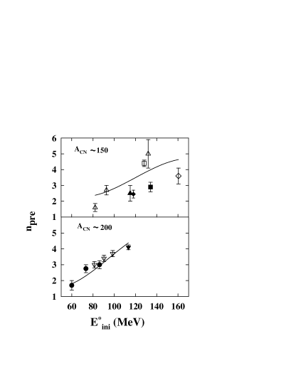
FIG. 1.: Prescission neutron multiplicities plotted as a function of the initial excitation energy $E^{*}_{ini}$ of the compound nuclei of masses A${}_{CN}\sim$ 150 (upper half), and A${}_{CN}\sim$ 200 (lower half). The solid curve is the present calculation. Different symbols correspond to different sets of experimental data, (ie, filled circle [19], open inverted triangle [19], filled inverted triangle [18], open triangle [19], filled triangle [20], open diamond [20], filled diamond [18], open square [18], filled square [18]).

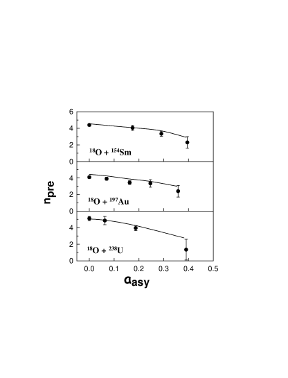
FIG. 2.: Prescission neutron multiplicity $n_{pre}$ as a function of fragment mass asymmetry $a_{asy}$for ${}^{18}O$ induced reactions on ${}^{154}Sm,\ ^{197}Au\ \rm{and}\ ^{238}U$. Filled circles correpond to the experimental data [18] and the solid curves are the present calculations.

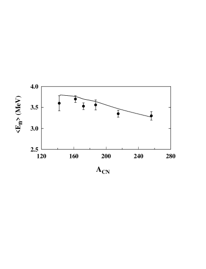
FIG. 3.: mean energy of the evaporated neutrons ($<E_{n}>$) plotted as a function of A_CN. The solid curves are the present calculations, and the filled circles are the corresponding data [18].

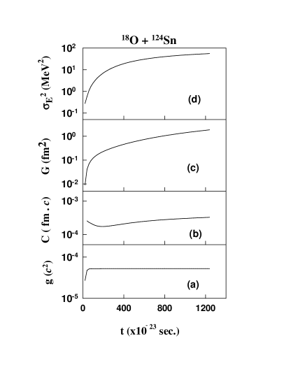
FIG. 4.: Variation of (a) $g(t)$, (b) $C(t)$, (c) $G(t)$ and (d) $\sigma^{2}_{E}$ as a function of time $t$ for the system ¹⁶O+¹²⁴Sn.

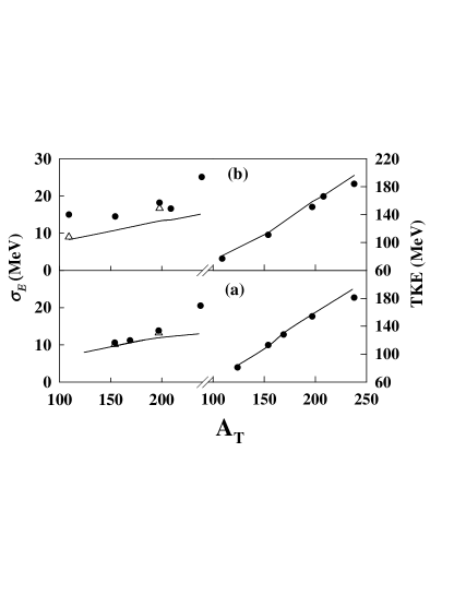
FIG. 5.: Variation of $\sigma_{E}$ and mean TKE as function of target mass number $A_{T}$, for (a) 158.8 MeV ¹⁸O , and (b) 288 MeV ¹⁶O induced fission reactions. Filled circles correspond to the experimental data [18] and solid curves are the present theoretical results. Open triangles are the values of $\sigma_{E}$ obtained using Eqs. (3.13) (see text).

FIG. 6.: Variation of predicted values of $\sigma_{E}$ as a function of fragment mass asymmetry, $a_{sym}=|A_{1}-A_{2}|/A_{CN}$.

REFERENCES

- [1] Abe, Y., Gregoire, C, Delagrange, H. : J. Phys. (Paris),47 32 (1986)
- [2] Abe, Y., Ayik, S., Reinhard, P. G., Suraud, E. : Phys. Rep. 275 49 (1996) and references therein
- [3] Frobrich, P., Gontchar, I. I., Mavlitov, N. D. : Nucl. Phys. A 556 281 (1993)
- [4] Pomorski, K., Bartel, J., Richert, J., Dietrich, K. : Nucl. Phys. A 605 87 (1996)
- [5] Kramers, A. : Physica 7 284 (1940)
- [6] Grange, P., Jun-Qing, Li., Weidenmuller, H. A. : Phys. Rev. C 27 2063 (1983)
- [7] Scheuter, F., Gregoire, C., Hofmann, H., Nix, J.R. : Phys. Lett. 149B 303 (1984)
- [8] Hofmann, H. : Phys. Rep. 284 137 (1997)
- [9] Van Kampen, N. G. : Stochastic processes in physics and chemistry (North-Holland : Amsterdam) (1991)
- [10] Dhara, A. K., Krishan, K., Bhattacharya, C., Bhattacharya, S. : Phys. Rev. C 57 2453 (1998)
- [11] Brack, M., Damgard, J., Jensen, A. S., Pauli, H. C., Strutinsky, V. M., Wong, C. Y. : Rev. Mod. Phys. 44 320 (1972)
- [12] Swiatecki, W.J. : Progress in Particle and Nuclear Physics ed. Wilkinson., D., (Pergamon, New York, 1980), Vol. 4, pp. 383; Randrup, J. : Nucl. Phys. A307 319 (1978)
- [13] Dhara, A. K., Bhattacharya, C., Bhattacharya, S., Krishan, K. : Phys. Rev. C 48 1910 (1993)
- [14] Bhattacharya, C., Bhattacharya, S., Krishan, K. : Phys. Rev. C 53 1012 (1996)
- [15] Davies, K. T. R., Sierk, A. J., Nix, J. R. : Phys. Rev. C 13 2385 (1976)
- [16] Feldmeier H 1987 Rep. Prog. Phys. 50 915
- [17] Pal, S. : Pramana-J. Phys 48 425 (1997)
- [18] Hinde, D. J., Hilscher, D., Rossner, H., Gebauer, B., Lehmann, M., Wilepert, M. : Phys. Rev. C 45, 1229 (1992).
- [19] Hinde, D. J., Charity, R. J., Foote, G. S., Leigh, J. R., Newton, J. O., Ogaza, S., Chatterjee, A. : Nucl. Phys. A452, 550 (1986).
- [20] Gavron, A., Gayer, A., Boissevain, J., Britt, H. C., Awes, T. C., Beene, J. R., Cheynis, B., Drain, D., Ferguson, R. L., Obenshain, F. E., Plasil, F., Young, G. R., Petitt, G. A., Butler, C. : Phys. Rev. C 35, 579 (1987).
- [21] Oganessian, Y. T., Lazarev, Y. A. : Treatise on heavy-ion science, vol. 4 (Ed. A. Bromley, Plenum Press) pp. 1 (1985)
- [22] Viola, V. E., Kwiatkowski, K., Walker, M. : Phys. Rev.C 31 1550 (1985)