Extraction of level density and $\gamma$ strength function from primary $\gamma$ spectra

Abstract

We present a new iterative procedure to extract the level density and the $\gamma$ strength function from primary $\gamma$ spectra for energies close up to the neutron binding energy. The procedure is tested on simulated spectra and on data from the ¹⁷³Yb(³He,$\alpha$)¹⁷²Yb reaction.

PACS number(s): 29.85.+c, 21.10.Ma, 25.55.Hp, 27.70.+q

1 Introduction

The $\gamma$ transitions of excited nuclei give rich information on nuclear properties. In particular, the energy distribution of the first emitted $\gamma$ rays from a given excitation energy reveals information on the level density at the excitation energy to which the nucleus decays, and the $\gamma$ strength function at the difference of those two energies. If the initial and final excitation energy belong to the continuum energy region, typically above 4 MeV of excitation energy for nuclei in the rare earth region, also thermodynamical properties may be investigated [1, 2].

Recently, the nuclear level density has become the object of new interest. There is strong theoretical progress in making calculations applicable to higher energies and heavier nuclei. In particular, the shell model Monte Carlo technique [3, 4] moves frontiers at present, and it is now mandatory to compare these calculations with experiments. Furthermore, the level density is essential for the understanding of the nucleon synthesis in stars. The level densities are input in large computer codes where thousands of cross sections are estimated [5].

Our present knowledge of the gross properties of the $\gamma$ strength function is also poor. The Weisskopf estimate which is based on single particle transitions, see e.g. [6], gives a first estimation for the strengths. However, for some measured $\gamma$ transitions the transition rate may deviate many orders of magnitude from these estimates. A recent compilation on average $\gamma$ transition strengths for M1, E1 and E2 transitions is given in Ref. [7]. The uncertainties concern the absolute strength as well as how the strength depends on the $\gamma$ transition energy. For E1 transitions, it is usually assumed that the energy dependency follows the GDR $(\gamma,\gamma^{\prime})$ cross section, however, this is not at all clear for low energy $\gamma$ rays.

In this work we describe a method to extract simultaneously the level density and $\gamma$ strength function in the continuum energy region for low spin (0-6 $\hbar$). The basic ideas and the assumptions behind the method were first presented in Ref. [8]. An implementation using an iterative projection technique, was first described in Ref. [9]. However, due to the existence of infinitely many solutions and the unfortunate renormalization of the primary $\gamma$ spectrum in every iteration step, this first implementation suffered from various severe problems, including divergence of the extracted quantities [10]. Several solutions of the convergence problem have been proposed and presented at different conferences, using approximate normalizations, but none of them yielding exact reproductions of test spectra. However, data using one of those approximate methods were published in Ref. [1]. Today, we consider the previous methods as premature, and we will present in the following a completely new, exact and convergent technique to extract level density and $\gamma$ strength function from primary $\gamma$ spectra.

2 Extracting level density and $\gamma$ strength function

2.1 Ansatz

We take the experimental primary $\gamma$ matrix $\Gamma(E_{i},E_{\gamma})$ as the starting point for this discussion. We assume that this matrix is normalized for every excitation energy bin $E_{i}$. This is done by letting the sum of $\Gamma$ over all $\gamma$ energies $E_{\gamma}$ from some minimum $\gamma$ energy $E_{\gamma}^{\mathrm{min}}$ to the maximum $\gamma$ energy $E_{i}$ at this excitation energy bin be unity, i.e.

$$\sum_{E_{\gamma}=E_{\gamma}^{\mathrm{min}}}^{E_{i}}\Gamma(E_{i},E_{\gamma})=1.$$ (1)

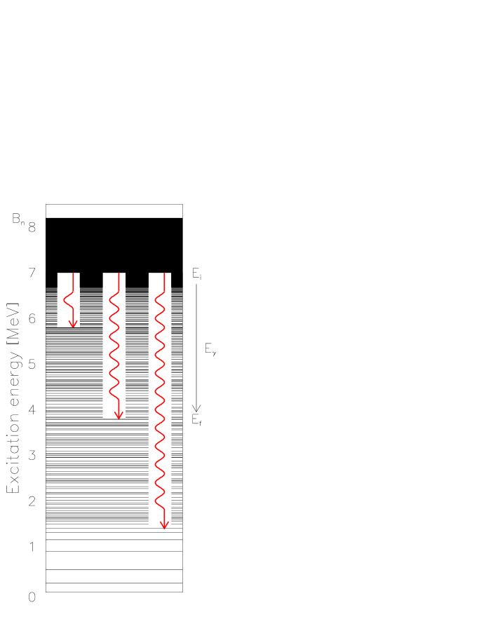
Figure 1: The $\gamma$ decay probability from an initial excitation energy $E_{i}$ in the statistical region is proportional to the level density at the final excitation energy $E_{f}$ and the $\gamma$ strength function at the $\gamma$ energy $E_{\gamma}=E_{i}-E_{f}$.

The $\gamma$ decay probability from the excitation energy $E_{i}$ to $E_{f}$ by a $\gamma$ ray with energy $E_{\gamma}=E_{i}-E_{f}$ in the continuum energy region is proportional to the level density $\varrho(E_{f})$ and a $\gamma$ energy dependent factor $F(E_{\gamma})$ [11, 12]. This ansatz is illustrated in Fig. 1. The experimental normalized primary $\gamma$ matrix $\Gamma$ can therefore theoretically be approximated by

$$\Gamma_{\mathrm{th}}(E_{i},E_{\gamma})=\frac{F(E_{\gamma})\,\varrho(E_{i}-E_{\gamma})}{\sum_{E_{\gamma}=E_{\gamma}^{\mathrm{min}}}^{E_{i}}F(E_{\gamma})\,\varrho(E_{i}-E_{\gamma})},$$ (2)

which also fulfills Eq. (1).

As it is shown in Appendix A, one can construct all solutions of Eq. (2) by applying the transformation given by Eq. (3) to one arbitrary solution, where the generators of the transformation $A$, $B$ and $\alpha$ can be chosen freely.

$$\tilde{\varrho}(E_{i}-E_{\gamma}) = \varrho(E_{i}-E_{\gamma})\,A\exp(\alpha\,(E_{i}-E_{\gamma})),$$ (3)

$$\tilde{F}(E_{\gamma}) = F(E_{\gamma})\,B\exp(\alpha\,E_{\gamma}),$$

2.2 Method

2.2.1 $0^{\mathrm{th}}$ order estimate

Since all possible solutions of Eq. (2) can be obtained by the transformation given by Eq. (3) of one arbitrary solution, we choose conveniently $\varrho^{(0)}=1$. With this choice, the $0^{\mathrm{th}}$ order estimate of $F$ is given by

$$\Gamma(E_{i},E_{\gamma})=\frac{F^{(0)}(E_{\gamma})}{\sum_{E_{\gamma}=E_{\gamma}^{\mathrm{min}}}^{E_{i}}F^{(0)}(E_{\gamma})}.$$ (4)

Summing over the excitation energy interval $E_{i}^{\mathrm{min}}\ldots E_{i}^{\mathrm{max}}$ while obeying $E_{i}\geq E_{\gamma}$ yields

$$\sum_{E_{i}=\max(E_{i}^{\mathrm{min}},E_{\gamma})}^{E_{i}^{\mathrm{max}}}\Gamma(E_{i},E_{\gamma})=F^{(0)}(E_{\gamma})\,\sum_{E_{i}=\max(E_{i}^{\mathrm{min}},E_{\gamma})}^{E_{i}^{\mathrm{max}}}\frac{1}{\sum_{E_{\gamma}=E_{\gamma}^{\mathrm{min}}}^{E_{i}}F^{(0)}(E_{\gamma})},$$ (5)

where the sum on the right hand side can be set to unity, giving

$$F^{(0)}(E_{\gamma})=\sum_{E_{i}=\max(E_{i}^{\mathrm{min}},E_{\gamma})}^{E_{i}^{\mathrm{max}}}\Gamma(E_{i},E_{\gamma}).$$ (6)

2.2.2 Higher order estimates

In order to calculate higher order estimates of the $\varrho$ and $F$ functions, we developed a least $\chi^{2}$ method. The basic idea of this method is to minimize

$$\chi^{2}=\frac{1}{N_{\mathrm{free}}}\,\sum_{E_{i}=\max(E_{i}^{\mathrm{min}},E_{\gamma})}^{E_{i}^{\mathrm{max}}}\sum_{E_{\gamma}=E_{\gamma}^{\mathrm{min}}}^{E_{i}}\left(\frac{\Gamma_{\mathrm{th}}(E_{i},E_{\gamma})-\Gamma(E_{i},E_{\gamma})}{\Delta\Gamma(E_{i},E_{\gamma})}\right)^{2},$$ (7)

where $N_{\mathrm{free}}$ is the number of degrees of freedom, and $\Delta\Gamma(E_{i},E_{\gamma})$ is the uncertainty in the primary $\gamma$ matrix. Since we assume every point of the $\varrho$ and $F$ functions as independent variables, we calculate $N_{\mathrm{free}}$ as

$$N_{\mathrm{free}}={\mathrm{ch}}(\Gamma)-{\mathrm{ch}}(\varrho)-{\mathrm{ch}}(F),$$ (8)

where ch indicates the number of data points in the respective spectra.

We minimize the reduced $\chi^{2}$ by letting all derivatives

$$\frac{\partial}{\partial\,F(E_{\gamma})}\chi^{2}=0\hskip 28.45274pt{\mathrm{and}}\hskip 28.45274pt\frac{\partial}{\partial\,\varrho(E_{i}-E_{\gamma})}\chi^{2}=0$$ (9)

for every argument $E_{\gamma}$ and $E_{i}-E_{\gamma}$ respectively. A rather tedious but straight forward calculation yields equivalence between Eqs. (9) and

$$F(E_{\gamma}) = \frac{\sum_{E_{i}=\max(E_{i}^{\mathrm{min}},E_{\gamma})}^{E_{i}^{\mathrm{max}}}\varrho(E_{i}-E_{\gamma})\,\varphi(E_{i},E_{\gamma})}{\sum_{E_{i}=\max(E_{i}^{\mathrm{min}},E_{\gamma})}^{E_{i}^{\mathrm{max}}}\varrho^{2}(E_{i}-E_{\gamma})\,\psi(E_{i},E_{\gamma})}$$ (10)

$$\varrho(E_{f}) = \frac{\sum_{E_{i}=\max(E_{i}^{\mathrm{min}},E_{f}+E_{\gamma}^{\mathrm{min}})}^{E_{i}^{\mathrm{max}}}F(E_{i}-E_{f})\,\varphi(E_{i},E_{i}-E_{f})}{\sum_{E_{i}=\max(E_{i}^{\mathrm{min}},E_{f}+E_{\gamma}^{\mathrm{min}})}^{E_{i}^{\mathrm{max}}}F^{2}(E_{i}-E_{f})\,\psi(E_{i},E_{i}-E_{f})},$$ (11)

where

$$\varphi(E_{i},E_{\gamma}) = \frac{a(E_{i})}{s^{3}(E_{i})}-\frac{b(E_{i})}{s^{2}(E_{i})}+\frac{\Gamma(E_{i},E_{\gamma})}{s(E_{i})\,\left(\Delta\Gamma(E_{i},E_{\gamma})\right)^{2}}$$ (12)

$$\psi(E_{i},E_{\gamma}) = \frac{1}{\left(s(E_{i})\,\Delta\Gamma(E_{i},E_{\gamma})\right)^{2}},$$ (13)

and

$$a(E_{i}) = \sum_{E_{\gamma}=E_{\gamma}^{\mathrm{min}}}^{E_{i}}\left(\frac{F(E_{\gamma})\,\varrho(E_{i}-E_{\gamma})}{\Delta\Gamma(E_{i},E_{\gamma})}\right)^{2}$$ (14)

$$b(E_{i}) = \sum_{E_{\gamma}=E_{\gamma}^{\mathrm{min}}}^{E_{i}}\frac{F(E_{\gamma})\,\varrho(E_{i}-E_{\gamma})\,\Gamma(E_{i},E_{\gamma})}{\left(\Delta\Gamma(E_{i},E_{\gamma})\right)^{2}}$$ (15)

$$s(E_{i}) = \sum_{E_{\gamma}=E_{\gamma}^{\mathrm{min}}}^{E_{i}}F(E_{\gamma})\,\varrho(E_{i}-E_{\gamma}).$$ (16)

Within one iteration, we first calculate the functions $a(E_{i})$, $b(E_{i})$ and $s(E_{i})$, using the previous order estimates for $\varrho$ and $F$. Using these three functions, we can calculate the matrices $\varphi(E_{i},E_{\gamma})$ and $\psi(E_{i},E_{\gamma})$. Further on, we calculate the actual order estimates of $\varrho$ and $F$ by means of Eqs. (10) and (11). Figure 2 shows where the sums in Eqs. (10) and (11) are performed.

2.2.3 Convergence properties

The method usually converges very well. However, in some cases the $\chi^{2}$ minimum is very shallow, and the chance exists, that the iteration procedure might fail. In order to enhance convergence of the method, we have restricted the maximum change of every data point in $\varrho$ and $F$ within one iteration to a certain percentage $P$. This means that the data point obtained in the actual iteration (new) is checked if it lies within the interval

$$\frac{\mathrm{old}}{(1+P/100)}\leq{\mathrm{new}}\leq(1+P/100)\cdot{\mathrm{old}},$$ (17)

determined by the data point from the previous iteration (old). In the case that the new data point lies outside this interval, it will be set to the value of the closest boundary.

Applying this method to some of our data, we have observed, that the smaller $P$ is chosen, the smaller $\chi^{2}$ gets in the end, when the procedure has reached its limit. The reason for this is, that more and more data points in $\varrho$ and $F$ will converge, while fewer and fewer points (typically at high energies $E_{\gamma}$ and $E_{f}$ where few counts are available) are oscillating between the two boundaries given by Eq. (17). Occasionally, we can choose $P$ so small that all data points will converge and no oscillating behavior can be seen. However, in some cases oscillating data points can not be avoided by any choice of $P$ which might indicate that the $\chi^{2}$ minimum is too shallow, or does not even exist, for some data points in $\varrho$ and $F$.

A small $P$ would lead to an accurate result but make a large number of iterations necessary, and a large $P$ would shorten the execution time of the procedure but affect the accurateness of the solution. We combine the advantages and avoid the disadvantages of the two concepts by letting $P$ become smaller as a function of the number of iterations. In our actual computer code [13], we have implemented a stepwise decrease of $P$ as shown in Table 1. The choices of $P$ as a function of the number of iterations is quite arbitrary, but we have achieved very good convergence for those spectra, where convergence properties without restrictions are rather fair.

In conclusion we have to stress, that the convergence properties of the method in many cases do not require any restrictions of the maximum variation of data points within one iteration. In those cases however, where restrictions are mandatory to achieve or enhance convergence, they will only affect a small percentage of the data points at high energies, where data in the primary $\gamma$ matrix are sparse and mainly erratically scattered. In those cases, where the restrictions of Table 1 would prove not to be satisfactory for convergence, the number of iterations or the value of $P$ can be changed, since the validity of the method does not rely on these values.

2.2.4 Error calculation

A huge effort has been made in order to estimate errors of the data points in $\varrho$ and $F$. Since the experimental primary $\gamma$ matrix has been obtained from raw data by applying an unfolding procedure [14] and a subtraction technique [15], error propagation through these methods is very tedious and has never been performed. In order to perform an error estimation of $\varrho$ and $F$, we first have to estimate the error of the primary $\gamma$ matrix data. A rough estimation yields

$$\Delta\Gamma=2\,\sqrt{(M_{1}+M_{2})\,\Gamma},$$ (18)

where $M_{1}$ denotes the number of first and higher generation $\gamma$ rays, and $M_{2}$ the number of second and higher generation $\gamma$ rays at one excitation energy bin $E_{i}$. We estimate those quantities roughly by

$$M_{1}=\max(1,M(E_{i}))\hskip 28.45274pt{\mathrm{and}}\hskip 28.45274ptM_{2}=\max(0,M(E_{i})-1),$$ (19)

where the multiplicity $M(E_{i})$ is given by a fit to the experimental data in Ref. [16]

$$M(E_{i})=0.42+4.67\,10^{-4}\,E_{i}-1.29\,10^{-8}\,E_{i}^{2},$$ (20)

and $E_{i}$ is given in keV. The motivation of Eq. (18) is that during the extraction method of primary $\gamma$ spectra of Ref. [15] the second and higher generation $\gamma$ ray spectrum, which has of the order $M_{2}\,\Gamma$ counts, is subtracted from the total unfolded $\gamma$ ray spectrum, which has of the order $M_{1}\,\Gamma$ counts. The errors of these spectra are roughly the square root of the number of counts. If we assume that these errors are independent from each other, the primary $\gamma$ spectra has an error of roughly $\sqrt{(M_{1}+M_{2})\,\Gamma}$. The factor 2 in Eq. (18) is due to the unfolding procedure and is quite uncertain. We assume this factor to be roughly equal the ratio of the solid angle covered by the CACTUS detector array of some 15% [17] to its photopeak efficiency of some 7% at 1.3 MeV [18]. We have however to apply a couple of minor corrections to Eq. (18).

Firstly, the first generation method [15] exhibits some methodical problems at low excitation energies. The basic assumption behind this method is that the $\gamma$ decay properties of an excited state is unaffected by its formation mechanism e.g. direct population by a nuclear reaction, or population by a nuclear reaction followed by one or several $\gamma$ rays. This assumption is not completely valid at low excitation energies, where thermalization time might compete with the half life of the excited state and the reactions used exhibit a more direct than compound character. This and some experimental problems like ADC threshold walk and bad timing properties of low energetic $\gamma$ rays, all described in Ref. [18], oblige us to exclude $\gamma$ rays below 1 MeV from the primary $\gamma$ spectra. For low energetic $\gamma$ rays above 1 MeV, we increase the error bars by the following rule. For each excitation energy bin $E_{i}$, we identify the channel with the maximum number of counts ch^max (this occurs typically between 2 and 3 MeV of $\gamma$ energy). This is also the channel with the highest error err^max, following Eq. (18). We then replace the errors of the channels ch below ch^max by

$${\mathrm{err}}={\mathrm{err}}^{\mathrm{max}}\,\left(1+1.0\cdot\frac{{\mathrm{ch}}^{\mathrm{max}}-{\mathrm{ch}}}{{\mathrm{ch}}^{\mathrm{max}}}\right).$$ (21)

This formula cannot be motivated by some simple handwaving arguments. We feel however, after inspecting several primary $\gamma$ matrices, that we estimate the systematic error of these spectra quite accurate.

Secondly, the unfolding procedure [14] exhibits some methodical problems at high $\gamma$ energies. Since the ratio of the photopeak efficiency to the solid angle covered by the CACTUS detector array drops for higher $\gamma$ energies, the counts at these energies are multiplied with significant factors in the unfolding procedure. Some channels might nevertheless turn out to contain almost zero counts, giving differences in counts between two neighboring channels by two orders of magnitude. Since the errors are estimated as proportional to the square root of the number of counts, the estimated errors of these channels do not reflect their statistical significance. In order to obtain comparable errors to neighboring channels we check the errors within one excitation energy bin from the $\gamma$ energy of $\sim$4 MeV and upwards. If the error drops by more than a factor 2, when going from one channel to the next higher one, we set the error of the higher channel equal to 50% of the error of the previous one. Also this rule cannot be motivated by a simple argumentation. It affects, however usually only a very small percentage of channels, and an inspection of several primary $\gamma$ spectra gives us confidence in our error estimation.

It is now very tedious to perform error propagation calculation through the extraction procedure. We therefore decided to apply a simulation technique to obtain reliable errors of the $\varrho$ and $F$ functions. For this reason, we add statistical fluctuations to the primary $\gamma$ matrix. For every channel in the primary $\gamma$ matrix, we choose a random number $r$ between zero and one. We then calculate $x$ according to

$$r=\frac{1}{\sqrt{2\pi}\,\sigma}\int_{-\infty}^{x}\exp(-\frac{(\xi-a)^{2}}{2\,\sigma^{2}})\,{\mathrm{d}}\xi,$$ (22)

where $a$ is the number of counts and $\sigma$ the error of this channel. By replacing the number of counts $a$ with $x$, we add a statistical fluctuation to this channel. This is done for all channels of the primary $\gamma$ matrix, and new $\varrho^{(s)}$ and $F^{(s)}$ functions are extracted, containing statistical fluctuations. This procedure is repeated 100 times, which gives reasonable statistics. The errors in $\varrho$ and $F$ are then calculated by

$$\Delta\varrho(E_{f}) = \frac{1}{\sqrt{100}}\,\sqrt{\sum_{i=1}^{100}[\varrho_{i}^{(s)}(E_{f})-\varrho(E_{f})]^{2}}$$ (23)

$$\Delta F(E_{\gamma}) = \frac{1}{\sqrt{100}}\,\sqrt{\sum_{i=1}^{100}[F_{i}^{(s)}(E_{\gamma})-F(E_{\gamma})]^{2}}.$$ (24)

2.2.5 Normalizing the level density to other experimental data

As pointed out above, all solutions of Eq. (2) can be generated from one arbitrary solution by the transformation given by Eq. (3). It is of course discouraging that an infinite number of equally good solutions exists, however by comparing to known data, we will be able to pick out the most physical one.

At low excitation energies up to typically 2 MeV for even even nuclei, we can compare the extracted level density to the number of known levels per excitation energy bin (for a comprehensive compilation of all known levels in nuclei see e.g. Ref. [19]). At the neutron binding energy, we can deduce the level density for many nuclei from available neutron resonance spacing data. The starting point is Eqs. (4) and (5) of Ref. [20]

$$\varrho(U,J) = \frac{\sqrt{\pi}}{12}\ \frac{\exp 2\sqrt{aU}}{a^{1/4}U^{5/4}}\ \frac{(2J+1)\exp(-(J+1/2)^{2}/2\sigma^{2})}{2\sqrt{2\pi}\sigma^{3}}$$ (25)

$$\varrho(U) = \frac{\sqrt{\pi}}{12}\ \frac{\exp 2\sqrt{aU}}{a^{1/4}U^{5/4}}\ \frac{1}{\sqrt{2\pi}\sigma},$$ (26)

where $\varrho(U,J)$ is the level density for both parities and for a given spin $J$, and $\varrho(U)$ is the level density for all spins and parities; $\sigma$ is the spin dependence parameter and $a$ the level density parameter. Assuming that $I$ is the spin of the target nucleus in a neutron resonance experiment, the neutron resonance spacing $D$ can be written as

$$\frac{1}{D}=\frac{1}{2}(\varrho(U_{n},J=I+1/2)+\varrho(U_{n},J=I-1/2)),$$ (27)

since all levels are accessible in neutron resonance experiments, and we assume, that both parities contribute equally to the level density at the neutron binding energy represented by $U_{n}$. Combining Eqs. (25), (26) and (27), one can calculate the total level density at the neutron binding energy

$$\varrho(U_{n})=\frac{2\sigma^{2}}{D}\ \frac{1}{(I+1)\exp(-(I+1)^{2}/2\sigma^{2})+I\exp(-I^{2}/2\sigma^{2})},$$ (28)

where $\sigma^{2}$ is calculated by combining Eqs. (9) and (11) of Ref. [20] i.e.

$$\sigma^{2}=0.0888\sqrt{aU_{n}}A^{2/3},$$ (29)

and $A$ is the mass number of the nucleus. It is assumed that $\sigma^{2}$ has an error of $\sim$10% due to shell effects [20]. One should also point out, that $U_{n}$ is given by $U_{n}=B_{n}-P$, where $B_{n}$ is the neutron binding energy and $P$ the pairing energy which can be found in Table III of Ref. [20] for many nuclei. Unfortunately, we cannot compare the calculated level density at the neutron binding energy directly with our extracted level density, since due to the omission of $\gamma$ rays below 1 MeV, the $\varrho$ function can only be extracted up to 1 MeV below the neutron binding energy. We will however extrapolate the extracted $\varrho$ function with a Fermi gas level density, obtained by combining Eqs. (26) and (29)

$$\varrho(U)=\frac{1}{12\sqrt{0.1776}A^{1/3}}\ \frac{\exp 2\sqrt{aU}}{a^{1/2}U^{3/2}}.$$ (30)

This is done by adjusting the parameters $A$ and $\alpha$ of the transformation given by Eq. (3) such, that the data fit the level density formula of Eq. (30) in an excitation energy interval between 3 and 1 MeV below $B_{n}$, where in most cases all parameters of Eq. (30) can be taken from Tables II and III of Ref. [20]. This semi experimental level density spanning from 0 MeV up to $B_{n}$ is then again transformed according to Eq. (3) such, that it fits the number of known levels up to $\sim$2 MeV and $\sim$1 MeV for even even and odd even nuclei respectively and simultaneously the level density deduced from neutron resonance spacing at $B_{n}$. We have to point out however, that after the fit to known data, the extrapolation does not have the functional form of Eq. (30) anymore, due to the transformation given by Eq. (3) applied to the semi experimental level density. Therefore, if necessary, a new extrapolation of the experimental data must be performed.

We have successfully implemented the new extraction method in a Fortran 77 computer code called rhosigchi [13]. The computer code was compiled under a Solaris 2.5.1 operating system running on a Dual UltraSPARC station with 200 MHz CPU. The execution time of one extraction is in the order of 10-20 s. The computer code has $\sim$1200 programming lines, excluding special library in and output routines.

3 Applications to spectra

3.1 Testing the method on theoretical spectra

The method has been tested on a theoretically calculated primary $\gamma$ matrix. The theoretical primary $\gamma$ matrix was obtained by simply multiplying a level density $\varrho$ to a $\gamma$ energy dependent factor $F$ according to Eq. (2). The level density was given by a backshifted Fermi gas formula

$$\varrho(U)=C\,U^{-3/2}\,\exp(2\sqrt{aU})$$ (31)

with $U=E_{f}-P$. Below the minimum at $U=9/4a$ a constant level density was used. The $\gamma$ energy dependent factor was chosen as

$$F(E_{\gamma})=C\,E_{\gamma}^{4.2}.$$ (32)

In addition, a “fine structure” was imposed on both functions, by scaling several $\sim$1 MeV broad intervals with factors around 1.5–5. Both model functions are shown in the upper half of Fig. 3. We extracted the $\varrho$ and $F$ functions from the theoretical primary $\gamma$ matrix using the excitation energy interval of 4 to 8 MeV and excluding all $\gamma$ rays below 1 MeV. In the lower panel of Fig. 3 we show the ratio of the extracted functions to the theoretical functions. After adjusting the extracted quantities with the transformation given by Eq. (3), we can state that the deviation from the input functions is smaller than one per thousand in the covered energy range of both functions. Tests of the old extraction method showed deviations of the order of 10% to 100% [21]. We therefore consider the new extraction method to be much more reliable.

3.2 Testing the method on ¹⁷²Yb spectra

We have tested the method on several experimental primary $\gamma$ spectra. We will in the following discuss a typical example; the ¹⁷³Yb(³He,$\alpha$)¹⁷²Yb reaction. The experiment was carried out at the Oslo Cyclotron Laboratory (OCL) at the University of Oslo, using a MC35 cyclotron with a beam energy of 45 MeV and a beam intensity of typically 1 nA. The experiment was running for two weeks. The target was consisting of a self supporting, isotopically enriched (92% ¹⁷³Yb) metal foil of 2.0 mg/cm² thickness. Particle identification and energy measurements were performed by a ring of 8 Si(Li) particle telescopes at 45^∘ with respect to the beam axis. The $\gamma$ rays were detected by an array of 28 $5^{\prime\prime}\times 5^{\prime\prime}$ NaI(Tl) detectors (CACTUS). More experimental details can be found in [17]. The raw data are unfolded, using measured response functions of the CACTUS detector array [14]. After unfolding, a subtraction method is applied to the particle $\gamma$ matrix in order to extract the first generation $\gamma$ matrix [15]. This primary $\gamma$ matrix is taken as the starting point for the extraction method presented here.

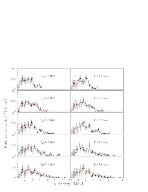
Figure 4: Normalized experimental primary $\gamma$ spectra with estimated errors (data points) and calculated primary $\gamma$ spectra from the extracted level density $\varrho$ and $\gamma$ energy dependent factor $F$ according to Eq. (2) (lines).

In Fig. 4, we show the normalized, experimental primary $\gamma$ spectra at ten different excitation energy bins (data points). The errors of the data points are estimated as explained above. The $\varrho$ and $F$ functions were extracted from the excitation energy interval 4-8 MeV, excluding all $\gamma$ energies smaller than 1 MeV. The lines are the calculated primary $\gamma$ spectra, obtained by multiplying the extracted level density $\varrho$ and the $\gamma$ energy dependent factor $F$ according to Eq. (2). One can see, that the lines follow the data points very well. It can also be seen that the errors of the data points are estimated reasonably giving a reduced $\chi^{2}$ of $\sim$0.4. Figure 4 is a beautiful example for the claim, that primary $\gamma$ spectra can be factorized according to the Axel Brink hypothesis [11, 12].

Figure 5 shows how the parameters $\alpha$ and $A$ of the transformation given by Eq. (3) can be determined in the case of the ¹⁷³Yb(³He,$\alpha$)¹⁷²Yb reaction. The extracted $\varrho$ function (data points) is compared to the number of known levels [19] per excitation energy bin (histogram) and to the level density at the neutron binding energy, calculated from neutron resonance spacing data [22] (data point in insert). The line in the insert is the extrapolation of the $\varrho$ function up to $B_{n}$ according to Section 2.2.5.

In the following, the extracted $\varrho$ and $F$ functions are discussed. Both functions were already published before, using the old extraction method and some fine structure discussed below, could already be seen in the previous publication [9]. Figure 6 shows the level density $\varrho$ and the relative level density, which is the level density, divided by an exponential fit to the data between the arrows. The parameters of the fit function

$$\varrho_{\mathrm{fit}}=C\exp(E/T)$$ (33)

are shown in the lower panel of the figure. In the relative level density one can see a small bump emerging at $\sim$2.7 MeV probably due to the quenching of pairing correlations [1, 2]. One can also see very nicely the onset of strong pairing correlations at 1.0–1.5 MeV of excitation energy.

In Fig. 7 the $\gamma$ energy dependent factor is shown (upper panel). On the lower panel, the same data are given, divided by a fit function of the form

$$F_{\mathrm{fit}}=C\,E_{\gamma}^{n}.$$ (34)

This function can be used as a parameterization of

$$F(E_{\gamma})=E_{\gamma}^{2\lambda+1}\,\sigma(E_{\gamma}),$$ (35)

where $\sigma(E_{\gamma})$ is the $\gamma$ strength function and $\lambda$ is the multipolarity of the $\gamma$ transition. The fit to the data was performed between the arrows, the fit parameter $n$ is given in the lower panel. Since other experimental data is very sparse, we did not scale $F$ in order to obtain absolute units. However, the extracted fit parameter $n$ is in good agreement with expectations from the tail of a GDR strength function at low $\gamma$ energies [8]. In the lower panel a merely significant bump at $\sim$3.4 MeV is visible, which we interpret as the Pigmy resonance.

4 Conclusions

In this work we have presented for the first time a reliable and convergent method to extract consistently and simultaneously the level density $\varrho$ and the $\gamma$ energy dependent function $F$ from primary $\gamma$ spectra. The new method, based on a least square fit, has been carefully tested on simulated $\gamma$ spectra as well as on experimental data. In order to normalize the data, we count known discrete levels in the vicinity of the ground state and use the level spacing known from neutron resonances at the neutron binding energy.

Compared to the previous projection method [9], the least square fit method gives the following advantages: The iteration converges mathematically. The reproduction of the input level densities and $\gamma$ strength functions in simulations is much better (almost exact). No tuning of the initial trial function is necessary to obtain a reasonable scaled level density, but the newly derived transformation properties of the solution enable the user to normalize the extracted quantities with known data. The reduced $\chi^{2}$ is estimated reasonably. The errors of the extracted quantities are estimated by statistical simulations.

We have used the new method to reanalyze previously published data and for the analysis of more recent data. Especially the ability to extract absolute values of the level density $\varrho$ enables us to perform several new applications [2, 23, 24].

5 Acknowledgments

The authors wish to thank A. Bjerve for interesting discussions. Financial support from the Norwegian Research Council (NFR) is gratefully acknowledged.

Appendix A Proof of Eq. (3)

The functional form of Eq. (2) opens for a manifold of solutions. If one solution of Eq. (2) is found, one can generally construct all possible solutions by the following transformation

$$\tilde{\varrho}(E_{i}-E_{\gamma}) = \varrho(E_{i}-E_{\gamma})\,g(E_{i}-E_{\gamma}),$$ (36)

$$\tilde{F}(E_{\gamma}) = F(E_{\gamma})\,f(E_{\gamma}).$$

The two functions $g$ and $f$ have to fulfill certain conditions, since the set of functions $\tilde{\varrho}$ and $\tilde{F}$ are supposed to form a solution of Eq. (2) i.e.

$$\Gamma_{\mathrm{th}}(E_{i},E_{\gamma})=\frac{F(E_{\gamma})\,\varrho(E_{i}-E_{\gamma})}{\sum_{E^{\prime}_{\gamma}=E_{\gamma}^{\mathrm{min}}}^{E_{i}}F(E^{\prime}_{\gamma})\,\varrho(E_{i}-E^{\prime}_{\gamma})}=\frac{\tilde{F}(E_{\gamma})\,\tilde{\varrho}(E_{i}-E_{\gamma})}{\sum_{E^{\prime}_{\gamma}=E_{\gamma}^{\mathrm{min}}}^{E_{i}}\tilde{F}(E^{\prime}_{\gamma})\,\tilde{\varrho}(E_{i}-E^{\prime}_{\gamma})}.$$ (37)

Inserting Eq. (36) one can easily deduce

$$f(E_{\gamma})\,g(E_{i}-E_{\gamma})\,\sum_{E^{\prime}_{\gamma}=E_{\gamma}^{\mathrm{min}}}^{E_{i}}\,F(E^{\prime}_{\gamma})\,\varrho(E_{i}-E^{\prime}_{\gamma})=$$

$$\sum_{E^{\prime}_{\gamma}=E_{\gamma}^{\mathrm{min}}}^{E_{i}}\,f(E^{\prime}_{\gamma})\,g(E_{i}-E^{\prime}_{\gamma})\,F(E^{\prime}_{\gamma})\,\varrho(E_{i}-E^{\prime}_{\gamma}).$$

Since the right side is independent of $E_{\gamma}$, also the left side must be independent of $E_{\gamma}$, thus the product of $f$ and $g$ must be a function of $E_{i}$ only yielding

$$f(E_{\gamma})\,g(E_{i}-E_{\gamma})=h(E_{i}).$$ (39)

This condition must of course hold for the case $E_{i}=E_{\gamma}$. Using the short hand notation $g(0)=A$, one obtains

$$A\,f(E_{\gamma})=h(E_{\gamma}).$$ (40)

Inserting this result in Eq. (39), one gets

$$f(E_{\gamma})\,g(E_{i}-E_{\gamma})=A\,f(E_{i}).$$ (41)

Analogously, the condition must hold for the case $E_{\gamma}=0$, and with $f(0)=B$, one obtains

$$B\,g(E_{i})=A\,f(E_{i}).$$ (42)

Inserting this result in Eq. (41), one finally gets

$$g(E_{\gamma})\,g(E_{i}-E_{\gamma})=A\,g(E_{i}).$$ (43)

We will now show, that the only solution of Eq. (43) is an exponential function. This proof will involve the limit of Eq. (43) for small $E_{\gamma}$. However, since $g$ is a function of only one variable and the variable $E_{i}$ is unrestricted in the proof, it will be valid for all arguments of $g$.

By expanding $g$ in Taylor series up to the first order in $E_{\gamma}$, one obtains

$$[A+g^{\prime}(0)\,E_{\gamma}]\,[g(E_{i})-g^{\prime}(E_{i})\,E_{\gamma}]=A\,g(E_{i}).$$ (44)

Neglecting second order terms in $E_{\gamma}$ and dividing by $E_{\gamma}$ one gets

$$g^{\prime}(0)\,g(E_{i})=A\,g^{\prime}(E_{i}).$$ (45)

Defining $\alpha=A/g^{\prime}(0)$, this differential equation is solved by

$$g(E_{i})=A\,e^{\alpha\,E_{i}}.$$ (46)

Using Eq. (42), we can easily deduce $f$ to be

$$f(E_{i})=B\,e^{\alpha\,E_{i}}.$$ (47)

Thus, we have proven the transformation given by Eq. (3) to be the most general way to construct all solutions of Eq. (2) from one arbitrary solution.

iteration	$P$ (%)	number of iterations	max. variation
1–5	20	5	$1.2^{5}\approx 2.49$
6–12	10	7	$1.1^{7}\approx 1.95$
13–21	5	9	$1.05^{9}\approx 1.55$
22–30	2.5	9	$1.025^{9}\approx 1.25$
31–50	1	20	$1.01^{20}\approx 1.22$
		$\sum=50$	$\prod\approx 11.46$

Table 1: $P$ as a function of the number of iterations. We have in the actual computer code implemented 50 iterations where $P$ is decreasing gradually from 20% to 1%. The maximum variation from the $0^{\mathrm{th}}$ order estimate any point can get is approximately a factor 11.

Figure 2: Performing the sum of Eqs. (10) and (11) along the thick lines. The shaded areas are usually excluded when extracting real data due to methodical problems (see text).

Figure 3: Theoretical level density $\varrho$ and $\gamma$ energy dependent factor $F$ used to calculate a primary $\gamma$ matrix (upper half). Ratio of extracted to theoretical $\varrho$ and $F$ functions (lower half).

Figure 5: Picking out the most physical solution of Eq. (2) by comparing the extracted level density $\varrho$ (data points) to the number of known levels per excitation energy bin (histogram) between the arrows, and the extrapolation of $\varrho$ up to $B_{n}$ (line in insert, see text) to the neutron resonance spacing data (data point in insert, see text).

Figure 6: Extracted normalized level density in ¹⁷²Yb (upper panel), and the same data divided by an exponential fit (lower panel, see text).

Figure 7: Extracted $\gamma$ energy dependent factor $F$ in ¹⁷²Yb (upper panel), and the same data divided by a fit function (lower panel, see text).

References

- [1] E. Melby, L. Bergholt, M. Guttormsen, M. Hjorth-Jensen, F. Ingebretsen, S. Messelt, J. Rekstad, A. Schiller, S. Siem, and S.W. Ødegård, Phys. Rev. Lett. 83, 3150 (1999)
- [2] A. Schiller, A. Bjerve, M. Guttormsen, M. Hjorth-Jensen, F. Ingebretsen, E. Melby, S. Messelt, J. Rekstad, S. Siem, and S.W. Ødegård, preprint nucl-ex/9909011
- [3] G.H. Lang, C.W. Johnson, S.E. Koonin, and W.E. Ormand, Phys. Rev. C48, 1518 (1993)
- [4] S.E. Koonin, D.J. Dean, and K. Langanke, Phys. Rep. 278, 1 (1997)
- [5] S. Goriely, Nucl. Phys. A605, 28 (1996)
- [6] A. Bohr and B.R. Mottelson, Nuclear Structure, (W.A. Benjamin, Inc., New York, Amsterdam, 1969), Vol. I, p. 389
- [7] W. Zipper, F. Seiffert, H. Grawe, and P. von Brentano, Nucl. Phys. A551, 35 (1993)
- [8] L. Henden, L. Bergholt, M. Guttormsen, J. Rekstad, and T.S. Tveter, Nucl. Phys. A589, 249 (1995)
- [9] T.S. Tveter, L. Bergholt, M. Guttormsen, E. Melby, and J. Rekstad, Phys. Rev. Lett. 77, 2404 (1996)
- [10] A. Bjerve, M. Guttormsen, E. Melby, J. Rekstad, A. Schiller, S. Siem, and T.S. Tveter, Department of Physics Report, University of Oslo, UiO/PHYS/97-08 (1997), p. 25
- [11] D.M. Brink, Ph.D. thesis, Oxford University, 1955
- [12] P. Axel, Phys. Rev. 126, 671 (1962)
- [13] A. Schiller, L. Bergholt, and M. Guttormsen, computer code rhosigchi, Oslo Cyclotron Laboratory, Oslo, Norway, 1999
- [14] M. Guttormsen, T.S. Tveter, L. Bergholt, F. Ingebretsen, and J. Rekstad, Nucl. Instrum. Methods A374, 371 (1996)
- [15] M. Guttormsen, T. Ramsøy, and J. Rekstad, Nucl. Instrum. Methods A255, 518 (1987)
- [16] T.S. Tveter, L. Bergholt, M. Guttormsen, and J. Rekstad, Nucl. Phys. A581, 220 (1995)
- [17] M. Guttormsen, A. Atac, G. Løvhøiden, S. Messelt, T. Ramsøy, J. Rekstad, T.F. Thorsteinsen, T.S. Tveter, and Z. Zelazny, Physica Scripta T32, 54 (1990)
- [18] A. Schiller, L. Bergholt, M. Guttormsen, E. Melby, S. Messelt, E.A. Olsen, J. Rekstad, S. Rezazadeh, S. Siem, T.S. Tveter, P.H. Vreim, and J. Wikne, Department of Physics Report, University of Oslo, UiO/PHYS/98-02 (1998), p. 31
- [19] R.B. Firestone and V.S. Shirley, Table of Isotopes, edition, (John Wiley & Sons, Inc., New York, Chichester, Brisbane, Toronto, Singapore, 1996), Vol. II
- [20] A. Gilbert and A.G.W. Cameron, Can. J. Phys. 43, 1446 (1965)
- [21] S. Siem, T.S. Tveter, L. Bergholt, M. Guttormsen, E. Melby, J. Rekstad, and A. Schiller, Department of Physics Report, University of Oslo, UiO/PHYS/97-08 (1997), p. 27
- [22] H.I. Liou, H.S. Camarda, G. Hacken, F. Rahn, J. Rainwater, M. Slagowitz, and S. Wynchank, Phys. Rev. C7, 823 (1973)
- [23] M. Guttormsen, M. Hjorth-Jensen, E. Melby, J. Rekstad, A. Schiller, and S. Siem, preprint nucl-ex/9910xxx
- [24] M. Guttormsen, A. Bjerve, M. Hjorth-Jensen, E. Melby, J. Rekstad, A. Schiller, and S. Siem, preprint nucl-ex/9910xxx