The Radiation Tail in $(e,e^{\prime}p)$ Reactions and Corrections to Experimental Data

We present a direct calculation of the cross section for the reaction ³He$(e,e^{\prime}p)$ including the radiation tail originating from bremsstrahlung processes. This calculation is compared to measured cross sections. The calculation is carried out from within a Monte Carlo simulation program so that acceptance-averaging effects, along with a subset of possible energy losses, are taken into account. Excellent agreement is obtained between our calculation and measured data, after a correction factor for higher-order bremsstrahlung is devised and applied to the tail. Industry-standard radiative corrections fail miserably for these data, and we use the results of our calculation to dissect the failure. Implications for design and analysis of experiments in the Jefferson-Lab energy domain are discussed.

I Introduction

The application of what are commonly called radiative corrections is an integral part of doing nuclear physics with beams of electrons. In an electron-scattering experiment, the probe is considered to be a virtual photon. This photon is exchanged between a beam electron and a target nucleus, thereby transferring energy and momentum to the target from the the electron, which is thereby scattered. Unfortunately, these electrons also copiously emit real photons which are not normally observed in experiments. Thus, either the theoretical calculations with which data are compared must include these processes (and they normally do not), or the data must somehow be corrected for these effects so that they can be compared to calculations which are based on single virtual-photon exchange. The standard choice is to “radiatively unfold” the experimental data, which generates a “corrected spectrum” that can be compared to theoretical calculations.

This paper reports on a study of how these real-photon processes affect measurements of $(e,e^{\prime}p)$ reactions on atomic nuclei. Our calculation takes the second approach, which is to radiatively correct a theoretical calculation so that it can be directly compared to uncorrected data. We compare a direct computation of a cross section, including the effects of photon emission, to a specific measurement of an $(e,e^{\prime}p)$ cross section[1, 2]. The results of applying the standard “radiative unfolding” procedure mentioned above to these data are also presented and discussed. The comparisons to this particular data set are unique in two ways:

1. the data appear to be well described in the plane-wave impulse approximation (PWIA), and

2. over most of the kinematic range of the measurement, the real-photon “radiative processes” are responsible for nearly the entire cross section.

The excellent PWIA reproduction of the cross section chosen for this study allowed us to use the PWIA in carrying out the complex calculations including radiative effects, enormously simplifying the task. The dominance of radiative strength enables us to make a true test of the real-photon emission model without worrying about accurately removing physical backgrounds.

This study is timely for several reasons. First, existing procedures for radiative corrections to data have been developed for experiments at relatively low ($<500$ MeV) electron beam energy. Refinements or overhauls of the procedure may be necessary to apply corrections for $(e,e^{\prime}p)$ experiments with higher-energy beams. The experiment studied here was carried out with a beam energy of 855 MeV, which bridges the gap between the energy domain studied by the labs active in the last decade (0.2–0.9 GeV) and the Jefferson Lab energy domain (0.8–6.0 GeV). Furthermore, a new class of experiments at Jefferson Lab begins to study $(e,e^{\prime}p)$ reactions in a kinematic domain where the cross sections are expected to be small and broadly peaked; radiative strength can easily swamp the “true” cross section in these cases. The design and analysis of these experiments should make careful studies of the radiative contributions to measured cross sections. Indeed, such an analysis was the genesis for the current work.

Finally, it became clear to us during the course of the project described here that the standard radiative-unfolding procedure used for the last decade is of an ad hoc nature; it is not based on rigorous theoretical arguments. We could only find one article published in a refereed journal [3] which specifically addressed radiative corrections for $(e,e^{\prime}p)$ reactions. This publication is either unknown to most experimentalists, or has been ignored for some reason, as a literature search uncovered only one reference [4] to this article, which argued that the corrections proposed in [3] were impractical since they make different assumptions about hadronic portions of the corrections, rendering data so corrected inconsistent with the world proton form-factor data.

All remaining works we could find addressing radiative corrections to experimental data were Ph.D. theses. Essentially all these works quote the Ph.D. thesis of Quint [5] as the primary reference. This thesis in turn quotes lecture notes of Penner [6] from a summer-school proceedings as a primary source, where radiative corrections for inclusive $(e,e^{\prime})$ reactions are discussed. These notes clearly state that the correction should be viewed as approximate; for example, they recommend an empirical adjustment of the calculated tail to give the best fit to the data, in cases where the radiation tail dominates the cross section. Aside from this problem and possible problems in adapting a formalism for $(e,e^{\prime})$ to correct $(e,e^{\prime}p)$ experiments, we have uncovered several questionable assumptions in this standard procedure, which we address in this article.

By contrast, we base our calculations on a published [7] first-order QED calculation for the radiation-tail cross section. Our work extends their result to kinematically-complete reactions and to higher-order bremsstrahlung radiation.

We are unaware of any previously-published similar study. We hope this paper will give some indication of how urgently new theoretical work is needed, and in what directions that work should proceed. Since the topic of radiative corrections is often viewed as an arcane subject which is best avoided, we present in the following sections a review of the relevant electromagnetic processes, a review of $(e,e^{\prime}p)$ phenomenology, and an explanation on how radiative effects distort $(e,e^{\prime}p)$ reaction data.

II Review of Radiative Processes in Electron Scattering

This section presents a review of the most important processes via which electrons emit real photons during interactions with nuclei. We emphasize here that this section is a review, meant to place these processes in the context of the reaction we study. Much of the conceptual work here, and formal work on bremsstrahlung presented in sec. V, can be found in classic articles [8, 9, 10].

FIG. 1.: Schematic diagram of the $(e,e^{\prime}p)$ reaction (in this case off an $A=4$ nucleus) to lowest electromagnetic order. An incident electron scatters from a target nucleus by exchange of a virtual photon, and a target proton is knocked out in the process. Symbols next to the various lines show the names given the four-momenta for each particle.

Fig. 1 is a schematic diagram of the $(e,e^{\prime}p)$ process to leading order in the electromagnetic coupling constant $\alpha$. It corresponds to the mental picture usually employed by an experimentalist designing or analyzing an experiment, since it probes the “signal” the experimenter usually wants to measure. It also corresponds to the usual plane-wave impulse approximation (PWIA) for $(e,e^{\prime}p)$ reactions. For the purpose of the study presented here, we have chosen a measurement on ³He which was performed in kinematics specifically chosen to optimize the accuracy of the PWIA. However, even in the limit that the PWIA holds for the hadronic portion of the process, the neglect of real-photon emission limits the accuracy of PWIA cross sections to at best 20% for electron energies above a few hundred MeV. An example diagram for this bremsstrahlung process is shown in Fig. 2. Here the spectator nucleons have been omitted from the picture for simplicity.

FIG. 2.: Example Feynman diagram of bremsstrahlung in $e$-$p$ scattering. A real photon is emitted from the outgoing electron. There are three other such diagrams, one each for the two proton legs and one for the incident electron leg.

The process in Fig. 2 is called internal bremsstrahlung since it occurs during the $(e,e^{\prime}p)$ reaction. A similar process (termed external bremsstrahlung) takes place in the Coulomb fields of other atoms in the target. A related process is not particularly relevant for understanding the effect of radiative processes on the $(e,e^{\prime}p)$ spectra, but must be included in any consistent calculation. This is the process in which two virtual photons are emitted, and an example diagram is shown in Fig. 3. Such diagrams are generally termed “virtual photon corrections.”

FIG. 3.: Example diagram for the virtual photon correction.

For fixed values of the four-momenta $e$ and $e^{\prime}$, we see that the value of the four-momentum transfer $q$ is changed in the diagram of Fig. 2 with respect to the leading-order process in Fig. 1. This in general leads to a change in the magnitude of the associated cross section (as does the vertex renormalization in Fig. 3). The extra emitted particle in Fig. 2 leads to a change in the asymptotic kinematics of the reaction as well. This creates an ambiguity; for a given measured event, it is impossible to tell whether the observed kinematics correspond to those of the reaction vertex, or to a different reaction-vertex situation accompanied by real photon emission.

We begin our discussion of this problem by summarizing the phenomenology of the $(e,e^{\prime}p)$ reaction in the next section. The section afterwards will give a quantitative description of the kinematic distortion due to the contributions of the diagram in Fig. 2. We present a rather complete summary of the kinematics, since discrepant conventions exist in the literature. In our discussions below, unless otherwise stated we use the following kinematic conventions:

• the four-vectors are denoted by the standard symbol for the associated particle, e.g. $A$ for the target four-momentum and $p^{\prime}$ for that of the knocked-out proton.

• $E_{g}$ and ${\bf p}_{g}$ refer to the relativistic energy and three-momentum of particle $g$, thus the four momentum for $g$ is $g=(E_{g},{\bf p}_{g})$. The magnitude of the three momentum is $p_{g}=\left|{\bf p}_{g}\right|$.

III Review of $(e,e^{\prime}p)$ Phenomenology

One of the main reasons why the $(e,e^{\prime}p)$ reaction has been so useful in nuclear physics is that it probes the properties of individual nuclear protons in a fairly direct manner. The measured particle momenta can be used to determine the energy and momentum that the struck proton had before the interaction. The only major assumption involved is that the interactions of the recoiling $(A-1)$ system and knocked-out proton are neglected (PWIA). While the PWIA is not sufficiently accurate for a quantitative analysis of $(e,e^{\prime}p)$ experiments, many experiments have shown [11] that the essential features are reasonably preserved and that a straightforward analysis is possible.

The probability of finding the “struck” proton of Fig. 1 (to which the four-momentum $q$ is transferred) is a function of two parameters: an energy (which we refer to as $\epsilon$) and a momentum (to which we refer as $\textstyle\rho$). Various equivalent conventions for $\epsilon$ exist; we use it to refer to the energy necessary to remove the proton from the nucleus. $\textstyle\rho$ refers to the momentum of the proton relative to the nuclear rest frame.

In our convention, $\epsilon$ consists of two parts: $\epsilon=S_{p}+E_{x}^{R}$. $S_{p}$ is the proton separation energy for the nucleus being bombarded, and $E_{x}^{R}$ is the excitation energy of the residual system “$R$” of $A-1$ nucleons.

Assuming that the PWIA holds, $\epsilon$ and $\textstyle\rho$ can be computed from the kinematic variables measured in $(e,e^{\prime}p)$ experiments. We begin by constructing a four-vector relation for the process (using the notation of Fig. 1):

$$e+A=e^{\prime}+R+p^{\prime}.$$ (1)

Assuming the reaction is carried out with a known beam energy, a fixed, pure target, and that the four-momenta of the scattered electron and knocked-out proton are measured in detectors, the kinematics are uniquely determined.

$$R=(E_{R},{\bf p}_{R})=(e-e^{\prime})+A-p^{\prime}.$$ (2)

The invariant mass of the $(A-1)$ system, $\sqrt{R^{2}}$, yields $m_{R}$; an experimental missing energy is computed as

$$E_{m}=m_{R}+m_{p}-m_{A}.$$ (3)

When PWIA holds, $\epsilon=E_{m}$. Similarly, an experimental missing momentum is defined as

$\displaystyle{\bf p}_{m}={\bf p}_{R}\,.$

When PWIA holds, the residual system is a spectator and thus must have had the same momentum ${\bf p}_{m}$ before the interaction. Since the nucleus as a whole was initially at rest, $\mathchoice{{\hbox{\boldmath$\displaystyle\rho$}}}{{\hbox{\boldmath$\textstyle\rho$}}}{{\hbox{\boldmath$\scriptstyle\rho$}}}{{\hbox{\boldmath$\scriptscriptstyle\rho$}}}=-{\bf p}_{m}=-{\bf p}_{R}$.

IV The Kinematical Effects of Bremsstrahlung

If we add a real photon as shown in Fig. 2 to one of the external legs in Fig. 1, we must account for it in the four-momentum conservation relation. Here we keep using $E_{m}$ and $p_{m}$ for the names of the measured quantities. We indicate by use of the extra subscript $v$ (e.g., ${\bf p}_{m,v}$) the corresponding quantity at the $qA$ (virtual-photon-nucleus) reaction vertex in the case that the actual reaction involved emission of a real photon.

The four-momentum conservation relation becomes

$$R=(e-e^{\prime})+A-p^{\prime}-\gamma,$$ (4)

where $\gamma=(k,{\bf k})$ refers to the real photon’s four-momentum. The three-vector component of this equation yields

$${\bf p}_{R,v} = {\bf q}-{\bf p}_{p^{\prime}}-{\bf k}\mbox{, so that}$$ (5)

$${\bf p}_{m,v} = {\bf p}_{m}-{\bf k}\,.$$ (6)

Thus the deduced missing momentum is ${\bf p}_{m}={\bf p}_{m,v}+{\bf k}$. The effect of the real photon emission on $E_{m}$ is not obvious when using four-momentum algebra; instead, we note that the zeroth component of (4) leads to

$$m_{R,v}+m_{p}-m_{A}=(E_{e}-E_{e^{\prime}}-T_{p^{\prime}}-T_{R,v})-k,$$ (7)

where $T$ refers to the particle’s kinetic energy and $k$ is the photon energy. The left-hand side of this relation is $E_{m,v}$, and the value in parentheses is, to a good approximation, what one would deduce for $E_{m}$ if one is ignorant of the photon emission. Thus $E_{m}\approx E_{m,v}+k$. The relation is approximate since one measures $T_{R}$, not $T_{R,v}$. However, the difference is in most cases quite small.

The bremsstrahlung-photon emission thus causes cross-section strength which would normally populate $(E_{m,v},p_{m,v})$ to instead be redistributed over a range of values $(E_{m},p_{m})$. Furthermore, the magnitude of this redistributed cross section will be modified since the momentum transfer $q$ will be changed. The redistributed strength is the origin of the well-known “radiation tail” of electron-scattering experiments. In general, the missing energy is simply increased by an amount equal to the radiated-photon energy. The missing momentum is shifted in a kinematic-dependent manner; the relative orientation of its vertex value ${\bf p}_{m,v}$ and that of the radiated photon ${\bf k}$ plays an important role. Fig. 4 illustrates how measured strength in a particular region of $(E_{m},p_{m})$ is fed, through the bremsstrahlung process, by various regions of $(E_{m,v},p_{m,v})$.

FIG. 4.: Example bremsstrahlung trajectories for ³He$(e,e^{\prime}p)$ in the $(E_{m,v},p_{m,v})$ plane for the kinematic settings given in Table I. Each line represents a trajectory through which strength from lower values of $E_{m,v}$ can feed into the selected bin of measured $(E_{m},p_{m})$. The four lines show paths for radiation occurring either on the incoming or outgoing electron leg, and also for two values of the deduced measured angle between ${\bf p}_{m}$ and ${\bf q}$, $\theta_{p_{m}-q}$.

A procedure (see Ref. [12] for a good discussion) has been developed for “radiatively correcting” $(e,e^{\prime}p)$ spectra. The procedure relies on the fact that in reactions for which $E_{m}$ is a minimum, there is no tail, only a reduction in the cross section due to the absence of that strength which has been moved into the tail at larger values of $E_{m}$. The procedure corrects cross section data by beginning with this minimum-$E_{m}$ bin, using the Schwinger correction to correct for the amount which has been lost to the tail. Then the tail itself is computed from this effectively “unradiated” cross section. The tail contribution from this bin is subtracted from all bins at larger missing energies. This procedure can be iterated bin-by-bin, moving from small $E_{m}$ to large, to remove the radiation tail.

Estimated uncertainties in the value of the correction are usually around 10–20%, which is acceptable when the correction itself is small. However, for experiments investigating the large-$E_{m}$ continuum cross section, the correction can become rather large, or the radiation tail can even dominate the cross section. In these cases, even a 10% uncertainty in the corrections can lead to essentially zero knowledge of the true “unradiated” cross section. It is important to be able to reliably estimate the strength of the radiation tail, so cases like this can be avoided during the planning stage of an experiment. In the following section, we describe the procedure for computing the cross section, including the radiation tail.

V Computation of $(e,e^{\prime}p)$ Cross Sections Including Radiative Processes

Our approach to direct computation of the $(e,e^{\prime}p)$ cross-section spectra, including bremsstrahlung processes, is based on the PWIA for the $(e,e^{\prime}p)$ reaction. The PWIA assumption is not a necessary one; however, a computation involving a more complete theory would be computationally much more intensive. The use of PWIA is well-motivated in our case since it works well for ³He$(e,e^{\prime}p)$, apart from an overall scaling factor; this has been observed in other experiments as well (see e.g. [13]). The basic program is as follows: a Monte-Carlo simulation is performed in which the four-momenta of the scattered electron and knocked-out proton are sampled over their respective acceptances. The kinematics for the $(e,e^{\prime}p)$ reaction vertex are then modified for bremsstrahlung processes according to the corresponding probability distributions. PWIA is finally used to compute the cross section, and any relevant jacobian factors are applied.

The data generated can then be used to form cross-section spectra using the same procedures applied when analyzing the experimental data. The use of Monte-Carlo simulation is important for an additional reason: the cross sections are often rapidly varying over the experimental acceptances. A calculation of cross-section spectra using only the kinematics corresponding to the centers of all the acceptances does not usually reproduce the experimental spectra. Indeed, when radiative corrections are applied to “deradiate” experimental data, often one of the biggest uncertainties stems from the acceptance-averaging assumption made. We will discuss this point in more detail later in the article. Our Monte-Carlo procedure allows for acceptance-averaging identical to that of the experiment.

A PWIA Cross Sections

The cross section for continuum $(e,e^{\prime}p)$ reactions, in the case where the residual $(A-1)$ system has a continuum of possible invariant masses $m_{R}$ is given by

$$\frac{d^{6}\sigma}{d\Omega_{e^{\prime}}d\omega d\Omega_{p^{\prime}}dE_{p^{\prime}}}=p_{p^{\prime}}E_{p^{\prime}}\sigma_{ep}S(E_{m},p_{m}).$$ (8)

$\omega$ is the electron energy loss, given in the laboratory system by $\omega=E_{e}-E_{e^{\prime}}$; equivalently it is the zeroth component of the four-vector momentum transfer $q=(\omega,{\bf q})$. $\sigma_{ep}$ is the elementary cross section for scattering of an electron from a moving nucleon. We used the “cc1” prescription [14] for this cross section. The differences between “cc1” and “cc2” at these kinematics is everywhere less than 3% [1]. Our calculation uses the Simon parameterization [15] of the nucleon electromagnetic form factors in the computation of $\sigma_{ep}$. $S(E_{m},p_{m})$ is the proton spectral function, which gives the probability of finding a proton in the nucleus with momentum $p_{m}$ and removal energy $E_{m}$.

The simulation samples particle momenta instead of energies, so the cross section must be adjusted before direct use by the program. For the continuum case, we have to apply the transformations $\omega\Rightarrow p_{e^{\prime}}$ and $E_{p^{\prime}}\Rightarrow p_{p^{\prime}}$. The resulting cross section used in the simulation is related to that of Eq. (8) by

$$\frac{d^{6}\sigma}{d\Omega_{e^{\prime}}dp_{e^{\prime}}d\Omega_{p^{\prime}}dp_{p^{\prime}}}=\frac{p_{p^{\prime}}}{E_{p}^{\prime}}\frac{d^{6}\sigma}{d\Omega_{e^{\prime}}d\omega d\Omega_{p^{\prime}}dE_{p^{\prime}}}.$$ (9)

In the case of reactions leaving the residual system in a discrete state, the cross section is given by

$$\frac{d^{5}\sigma}{d\Omega_{e^{\prime}}d\Omega_{p^{\prime}}dp_{e^{\prime}}}=\frac{p_{p^{\prime}}E_{p^{\prime}}\sigma^{\textrm{cc}1}_{ep}n(p_{m})}{R}.$$ (10)

For these reactions $E_{m}$ has a definite value $E_{\alpha}$, so $S(E_{m},p_{m})$ is replaced by the momentum distribution $n(p_{m})$, where

$$S(E_{m},p_{m})=n(p_{m})\delta(E_{m}-E_{\alpha}).$$ (11)

$R$ is the “recoil factor” (really a jacobian factor transforming $E_{p^{\prime}}\Rightarrow E_{m}$), and is given by

$$R=1-\frac{E_{p^{\prime}}}{E_{R}}\frac{{\bf p}_{R}\cdot{\bf p}_{p^{\prime}}}{\left|{\bf p}_{p^{\prime}}\right|^{2}}.$$ (12)

Here we have not included the extra subscript $v$ on the kinematic quantities, but it should be understood when evaluating the radiative cross sections later in this section, that the hadronic cross section terms must be evaluated at the hadronic-vertex kinematics. Subscripts have been added in that section as a reminder.

So far, we have only studied light nuclei with only one possible discrete transition (the $A-1$ ground state), so our complete simulation consists of a sum of one discrete simulation and one continuum simulation. These two simulations are each themselves composed of two simulations to handle the different pieces of the radiation tail. The procedure is straightforward to extend to more complicated situations including additional bound-state channels.

B External Bremsstrahlung

External bremsstrahlung is relatively simple to include. The simulation program contains a model for the actual reaction target. For each event, an interaction vertex is chosen randomly within the intersection of the beam and target volumes. After this choice, the amount of target material traversed by the electron before and after the reaction is computed. The electron is transported through each material (e.g., target cell walls or target gas). After each traversal, a new electron energy is generated directly from sampling Tsai’s distribution [10] for bremsstrahlung from a thin radiator:

$$I_{\textrm{ext}}(E_{0},k,t) = \frac{bt}{\Gamma(1+bt)}\left(\frac{k}{E_{0}}\right)^{bt}\times$$ (14)

$$\frac{1}{k}\left(1-\frac{k}{E_{0}}+\frac{3}{4}\left(\frac{k}{E_{0}}\right)^{2}\right).$$

Here $k$ is the radiated photon energy (or energy lost by the electron), $E_{0}$ is the energy of the electron upon entering the radiator material, $t$ is the thickness of the radiator material in radiation-length units, $b$ is Tsai’s bremsstrahlung parameter (see Eq. (4.3) of [10]), and $\Gamma$ is the usual gamma function.

C Internal Bremsstrahlung

Internal bremsstrahlung is included using the cross sections for first-order photon emission derived by Borie and Drechsel [7]. Their derivation made use of the peaking approximation, which assumes that bremsstrahlung photons are only emitted along either the incident beam direction, or the direction of the scattered electron’s momentum. A critical review of the peaking approximation can be found in [9]. We use their results to estimate the validity of the peaking approximation for our kinematics, and find that it should be accurate to better than 1%. We note here that it is difficult to make blanket statements about the peaking approximation, except that it becomes increasingly worse for larger bremsstrahlung-photon energies.

The Borie-Drechsel cross section was also derived specifically for $(e,e^{\prime}p)$ reactions to the $(A-1)$ continuum. Part of the present work is an extension of that formalism to processes in which the $(A-1)$ system is in a discrete state. We also present a derivation of a correction factor which accounts for higher-order bremsstrahlung processes.

For the continuum case, there is complete kinematical freedom for all particles, as long as the invariant mass of the $(A-1)$ system is large enough to be above the particle-emission threshold of the $(A-1)$ nucleus. The simulation then samples all kinematic variables (the scattered-electron three-momentum, the ejected proton three-momentum, and the emitted photon momentum). In this case, the relevant cross section is given by Ref. [7], but we repeat it here with different notation and in a form consistent with our results for the discrete case. Unless otherwise specified, all kinematic quantities refer to the asymptotic situation, i.e., what would be assigned if one was not aware that a real photon had been emitted. These cross sections have a two-term structure which arises from the peaking approximation. The first term below corresponds to “preradiation” (photon emission along the beam direction) and the second term corresponds to “postradiation”.

$$\frac{d^{7}\sigma}{dkd\omega dp_{p^{\prime}}d\Omega_{e^{\prime}}d\Omega_{p^{\prime}}} = f_{\mathrm{mp}}\Bigl{\{}\Bigl{(}\frac{dr}{dk}\Bigr{)}_{e}\,\,\frac{d^{6}(e-\gamma,e^{\prime})}{d\omega_{v}dp_{p^{\prime}}d\Omega_{e^{\prime},v}d\Omega_{p^{\prime}}}$$ (16)

$$+\Bigl{(}\frac{dr}{dk}\Bigr{)}_{e^{\prime}}\,\,\frac{d^{6}(e,e^{\prime}+\gamma)}{d\omega_{v}dp_{p^{\prime}}d\Omega_{e^{\prime},v}d\Omega_{p^{\prime}}}\Bigr{\}}.$$

The factor $f_{\mathrm{mp}}$ corresponds to our “multi-photon” correction factor which we will discuss later; $f_{\mathrm{mp}}=1$ corresponds to the result published in [7]. In this section, we can use $k$ for both the energy and the momentum of $\gamma$ since it is a real photon. The $dr/dk$ terms are essentially jacobian factors for the photon emission. They will be given below. Finally, the two cross sections on the right-hand side of Eq. (16) are the usual “unradiated” cross sections, and must be evaluated at the vertex values. This is why for example the first cross section is a function of $e-\gamma$ (the beam four-momentum adjusted for photon emission before the interaction) rather than of $e$.

For the discrete case, the kinematics are over-determined. Since both the scattered electron and ejected proton are “detected” in the simulation, but the photon is not, we sample over the six-dimensional $({\bf p}_{e^{\prime}},{\bf p}_{p^{\prime}})$ space. For each point in this space, photon energies can be chosen which belong to this coordinate and as well result in the correct invariant mass of the $(A-1)$ system. $k_{e}$ is the real-photon energy in the case that the photon is emitted along the direction of the incident electron, and $k_{e^{\prime}}$ is that for the case of photon emission along the scattered-electron direction. These values are in general not the same (as opposed to the continuum case of Eq. (16), where the values of $k$ were the same).

$$k_{e}=\frac{\Lambda^{2}-m_{R}^{2}+2{\bf p}_{e}\cdot({\bf p}_{p^{\prime}}+{\bf p}_{e^{\prime}}-{\bf p}_{e}/2)-({\bf p}_{p^{\prime}}+{\bf p}_{e^{\prime}})^{2}}{2[\Lambda+\widehat{{\bf p}}_{e}\cdot({\bf p}_{p^{\prime}}+{\bf p}_{e^{\prime}}-{\bf p}_{e})]}$$ (17)

$$k_{e^{\prime}}=\frac{\Lambda^{2}-m_{R}^{2}-2{\bf p}_{e^{\prime}}\cdot({\bf p}_{p^{\prime}}+{\bf p}_{e^{\prime}}/2-{\bf p}_{e})-({\bf p}_{p^{\prime}}-{\bf p}_{e})^{2}}{2[\Lambda+\widehat{{\bf p}}_{e^{\prime}}\cdot({\bf p}_{p^{\prime}}+{\bf p}_{e^{\prime}}-{\bf p}_{e})]}$$ (18)

$$\Lambda=m_{A}+\omega-E_{p^{\prime}}$$ (19)

$$\widehat{{\bf p}}_{e,e^{\prime}}=\frac{{\bf p}_{e,e^{\prime}}}{|{\bf p}_{e,e^{\prime}}|}$$ (20)

Again here $\omega$ refers to the observed, asymptotic value, not that at the vertex. Similarly, $\Lambda$ includes the total energy of both the recoiling hadronic system and the radiated photon since $\omega$ is the asymptotic value.

The associated cross section is

$$\frac{d^{6}\sigma}{d\omega dp_{p^{\prime}}d\Omega_{e^{\prime}}d\Omega_{p^{\prime}}} = f_{\mathrm{mp}}\Bigl{\{}\Bigl{|}\frac{dk}{dp_{p^{\prime}}}\Bigr{|}_{e}\Bigl{(}\frac{dr}{dk}\Bigr{)}_{e}\frac{d^{5}\sigma(e-\gamma_{e},e^{\prime})}{d\omega_{v}d\Omega_{e^{\prime},v}d\Omega_{p^{\prime}}}$$ (22)

$$+\Bigl{|}\frac{dk}{dp_{p^{\prime}}}\Bigr{|}_{e^{\prime}}\Bigl{(}\frac{dr}{dk}\Bigr{)}_{e^{\prime}}\frac{d^{5}\sigma(e,e^{\prime}+\gamma_{e^{\prime}})}{d\omega_{v}d\Omega_{e^{\prime},v}d\Omega_{p^{\prime}}}\Bigr{\}}.$$

$f_{\mathrm{mp}}$ has the same meaning as in the preceding paragraph. $\gamma_{e,e^{\prime}}$ are the four-momenta corresponding to $k_{e,e^{\prime}}$. The above result (setting $f_{\mathrm{mp}}=1$ for the moment) was generated by substituting Eq. (8), coupled with the discrete-final-state expression for the spectral function (Eq. (11)), into the Borie-Drechsel formula for the radiation tail (Eq. (16)). The integral over $dE_{m,v}$ was formally carried out by converting it, with the help of appropriate jacobian factors, to an integral over $dk$. The kinematical factors for photon emission, one each for pre- and postradiation, are given by

$$\Bigl{(}\frac{dr}{dk}\Bigr{)}_{e} = \frac{\alpha}{\pi k_{e}}\,\,\frac{E_{e}^{2}+(E_{e}-k_{e})^{2}}{E_{e}^{2}}\ln\frac{2E_{e}}{m_{e}}$$ (23)

$$\Bigl{(}\frac{dr}{dk}\Bigr{)}_{e^{\prime}} = \frac{\alpha}{\pi k_{e^{\prime}}}\,\,\frac{(E_{e^{\prime}}+k_{e^{\prime}})^{2}+E_{e^{\prime}}^{2}}{(E_{e^{\prime}}+k_{e^{\prime}})^{2}}\ln\frac{2E_{e^{\prime}}}{m_{e}}$$ (24)

In the continuum case, $k_{e}$ and $k_{e^{\prime}}$ are identical (the sampled photon energy). The jacobian factors transforming the cross section from differential in $k_{e,e^{\prime}}$ to differential in $p_{p^{\prime}}$ are

$$\Bigl{|}\frac{dk}{dp_{p^{\prime}}}\Bigr{|}_{e,e^{\prime}}=\frac{A_{e,e^{\prime}}+C_{e,e^{\prime}}p_{p^{\prime}}/E_{p^{\prime}}}{B_{e,e^{\prime}}-C_{e,e^{\prime}}}$$ (25)

where

$$A_{e}=p_{p^{\prime}}+\widehat{{\bf p}}_{p^{\prime}}\cdot[{\bf p}_{e^{\prime}}-({\bf p}_{e}-{\bf k}_{e})]$$ (26)

$$A_{e^{\prime}}=p_{p^{\prime}}+\widehat{{\bf p}}_{p^{\prime}}\cdot[({\bf p}_{e^{\prime}}+{\bf k}_{e^{\prime}})-{\bf p}_{e}]$$ (27)

$$B_{e}=(E_{e}-k_{e})-\widehat{{\bf p}}_{e}\cdot({\bf p}_{e^{\prime}}+{\bf p}_{p^{\prime}})$$ (28)

$$B_{e^{\prime}}=-(E_{e^{\prime}}+k_{e^{\prime}})+\widehat{{\bf p}}_{e^{\prime}}\cdot({\bf p}_{e}-{\bf p}_{p^{\prime}})$$ (29)

$$C_{e,e^{\prime}}=\Lambda-k_{e,e^{\prime}}$$ (30)

$$\widehat{{\bf p}}_{p^{\prime}}=\frac{{\bf p}_{p^{\prime}}}{|{\bf p}_{p^{\prime}}|}$$ (31)

D Schwinger Correction

The internal-bremsstrahlung cross section given above becomes singular as the radiated-photon energy goes to zero. Hence it can not be used to provide the complete radiated cross section. The classic technique is to choose a cutoff energy $\Delta E$ which is comparable to the experimental energy resolution; a radiation tail is generated with photon energies between $\Delta E$ and the full energy of the radiating electron. The remaining cross section in the originating kinematic bin (i.e., the cross section for this particular reaction where the total energy radiated away by real photons is less than $\Delta E$) is calculated by computing the cross section without the internal bremsstrahlung graphs, and then reducing this cross section to account for that strength which was moved into the radiation tail. This reduction factor is called the Schwinger correction. For brevity, in discussions below we will refer to the strength remaining in the original kinematic bin as the “unradiated strength”.

The formalism we use for the Schwinger correction is due to Penner [6], and is written as

$$C_{\mathrm{S}chw}=e^{-\delta_{r}}(1-\delta_{v}),$$ (32)

where $\delta_{r}$ is the first-order correction for internal bremsstrahlung. Penner’s formulation is based on that of Maximon (the expression at the bottom of p. 199 of ref. [16]) with the addition of kinematic recoil corrections proposed by Tsai [17]. Furthermore, the part of this correction corresponding to real-photon emission ($\delta_{r}$) has been exponentiated. Exponentiation of this first-order correction was suggested by Schwinger [8] as a means of accounting for higher-order (multiple-photon) bremsstrahlung. $\delta_{v}$ is the correction for virtual-photon loops at the reaction vertex. The two $\delta$ factors are given by

$$\delta_{r} = \frac{\alpha}{\pi}\Bigl{(}\ln\frac{Q^{2}}{m_{e}^{2}}-1\Bigr{)}\ln\Bigl{[}\frac{\kappa}{\zeta^{2}}\frac{E_{e}E_{e^{\prime}}}{(\Delta E)^{2}}\Bigr{]}$$ (33)

$$\delta_{v} = \frac{\alpha}{\pi}\Bigl{[}\frac{28}{9}-\frac{13}{6}\ln\frac{Q^{2}}{m_{e}^{2}}+\frac{1}{2}\ln^{2}\frac{E_{e}}{E_{e^{\prime}}}+\frac{\pi^{2}}{6}$$ (35)

$$-L_{2}\Bigl{(}\cos^{2}\frac{\theta_{e^{\prime}}}{2}\Bigr{)}\Bigr{]}$$

with the “recoil factors” given by

$$\zeta = 1+\frac{E_{e}}{M_{A}}(1-\cos\theta_{e^{\prime}})\text{\, and}$$ (36)

$$\kappa = 1+\frac{\omega}{M_{A}}(1-\cos\theta_{e^{\prime}})\,.$$ (37)

$L_{2}(x)$ is the Spence function defined by

$\displaystyle L_{2}(x)=-\int_{0}^{x}\frac{\ln(1-y)}{y}dy\,.$

Finally, $Q^{2}$ denotes the standard square of the four-momentum transfer, $Q^{2}=-\left(e-e^{\prime}\right)^{2}$.

This version of the Schwinger correction does not account for possible real-photon emission by the hadrons involved in the reaction. Makins [4] has noted that this process may begin to become important momentum transfers $Q^{2}>1$ GeV/c. Penner’s correction also omits all hadron self-energy and vertex-renormalization diagrams. The assumption implicit in this approach is that such diagrams become part of what one calls the “electromagnetic form factor” of the struck hadron.

VI Simulation Framework

The models for $(e,e^{\prime}p)$ cross sections in PWIA, for external bremsstrahlung, and for internal bremsstrahlung were implemented in the simulation code AEEXB [18, 19]. This code also includes facilities enabling a fairly complete simulation of experimental factors such as target geometry, beam energy dispersion, ionization energy losses, and experimental acceptances. All these facilities were used in order to make the comparison as realistic as possible. For practical reasons, certain classes of ionization energy losses were not included. Since our electron energies are above the critical energy (for which radiative energy loss processes become more important than those due to atomic ionization), the ionization losses had a negligible effect on our results. Ion-optical magnetic transport is also possible in AEEXB, using an interface to the standard ion-optics program TURTLE [19, 20], but was neither necessary nor used for the current project.

A complete cross-section simulation including the radiation tail consists of several distinct pieces which must be combined at the end to obtain the final result. The framework is sketched here; readers wishing to see a more detailed explanation should refer to [21]. The discussion below makes the simplifying assumption that the final state space for the residual $(A-1)$ nucleus consists of one discrete state plus a continuum; this condition is satisfied for the reaction with which we compare, ${}^{3}\mbox{He}(e,e^{\prime}p)$. Multiple discrete states would be straightforward to implement. The spectral function used for ³He comes from the INFN/Rome group [22, 23].

A complete simulation consists of the following individual simulation runs:

1. two-body breakup with external bremsstrahlung. This run handles computation of the “unradiated” part of the cross section (see Sec. V D). No internal bremsstrahlung is computed; rather, the computed PWIA cross sections are reduced by the Schwinger correction to account for the fraction which will be redistributed into the internal-bremsstrahlung tail. Sampling is performed in $({\bf p}_{e^{\prime}},\theta_{p},\phi_{p})$; the constraint of a definite $(A-1)$ final-state mass provides the solution for $p_{p^{\prime}}$. External bremsstrahlung is allowed before the $(e,e^{\prime}p)$ vertex (modifying the beam energy) and afterwards (modifying the scattered-electron energy). The external-bremsstrahlung distribution is directly sampled, obviating the need for a cutoff correction.

2. two-body breakup with internal and external bremsstrahlung. This run handles the part of the cross section which has been redistributed into the internal radiation tail. For each event, six variables are sampled $({\bf p}_{e^{\prime}},{\bf p}_{p^{\prime}})$. First, external bremsstrahlung is computed along the incident electron direction (possibly modifying the incident electron energy). Then solutions are found for the radiated-photon energies corresponding to internal radiation along either the incident or scattered electron directions. The cross section is computed according to Eq. (22). Finally, external bremsstrahlung is computed along the scattered electron direction (possibly modifying the detected electron energy). Here only the virtual-photon part $(1-\delta_{v})$ of the Schwinger correction is applied since the radiative tail corresponding to $\delta_{r}$ is what we are computing.

3. continuum breakup with external bremsstrahlung. This piece is similar to case 1 above, except that events are sampled in six kinematic variables $({\bf p}_{e^{\prime}},{\bf p}_{p^{\prime}})$ since there is a continuum of possible $(A-1)$ final states.

4. continuum breakup with both internal and external bremsstrahlung. This simulation is similar to that of case 2 above, except that due to the complete kinematic freedom in the final state, the photon energy is constrained only to be larger than $\Delta E$ (the experimental resolution). Therefore, seven variables are sampled, the radiated-photon energy being the seventh.

5. detection volume simulation. This simulation is standard procedure for determining what fraction of the six-dimensional acceptance in $({\bf p}_{e^{\prime}},{\bf p}_{p^{\prime}})$ can contribute to any given bin in a cross-section spectrum. The results of this piece are used to properly normalize the simulated spectra when producing cross section results. No energy losses effects are included, since this part of the simulation only measures the relative probability of detection of various kinematical configurations (regardless of their origin).

The simulations, when properly weighted by sampling volumes and numbers of trials, are combined to form simulated cross sections. The cross sections can be plotted as the same sort of spectra shown in experimental papers, by sorting the simulated events into histograms in the same way an experimenter would sort data.

VII Experimental Data

The data with which we compare our simulations was acquired with the three-spectrometer detector setup at the MAMI accelerator facility in Mainz [24, 25]. Two of these spectrometers were used to detect scattered electrons and knocked-out protons; the third served as a luminosity monitor. A cryogenic gas target provided the ${}^{3}{\mathrm{H}e}$ target nuclei. The experiment measured cross sections for the reaction ${}^{3}{\mathrm{H}e}(e,e^{\prime}p)$ in a variety of kinematic settings. For more information on the experiment and its physics goals, the reader can consult [1]; here we focus only on the essentials needed for the radiation-tail comparison. The kinematical settings and experimental acceptances for the data discussed here are given in Table I.

Beam Energy	855 MeV
Electron Scattering Angle	52.4 deg
Scattered Electron Momentum (central)	627 MeV/c
Momentum Acceptance	$\pm 9.5$%
Nominal Electron Solid Angle	20 msr
Proton Detection Angle	-46.41 deg
Proton Momentum (central)	661 MeV/c
Momentum Acceptance	$\pm 7.4$%
Nominal Proton Solid Angle	4.8 msr
Experimental $E_{m}$ Resolution ($\Delta E$)	0.4 MeV

TABLE I.: Kinematic Settings for Experimental Data

One question which must be addressed in this study is “how well can the PWIA model describe the reaction?” If the description is not favorable, further work is useless since our model computes the basic $(e,e^{\prime}p)$ cross section in PWIA.

FIG. 5.: Experimental and Theoretical Momentum Distributions for ${}^{3}{\mathrm{H}e}(e,e^{\prime}p)^{2}{\mathrm{H}}$. Experimental distributions are shown for three different electron beam energies; the figure of 0.84 in the text refers to the ratio of the 855 MeV experimental distribution to the theoretical distribution.

Figure 5 shows the measured experimental momentum distribution $n_{\mathrm{exp}}=\sigma/(K\sigma_{ep})$ where $K$ stands for the kinematical factors in Eq. (10). The experimental cross section $\sigma$ above has been radiatively corrected using the traditional technique, which has been shown to work well in this experiment [1] for excitation energies less than 20 MeV. After radiative correction, the two-body peak could be cleanly resolved from the continuum and a cross section assignment is straightforward.

The momentum distribution is compared to the theoretical two-body breakup spectral function [22, 23] $S(S_{p},p_{m})$. $S_{p}$ is the single-proton separation energy and corresponds to ${}^{3}{\mathrm{H}e}\longrightarrow p\,\,+\,\,^{2}{\mathrm{H}}$. Aside from an overall scaling factor of 0.84, the theoretical spectral function is in good agreement with the data. We interpret this agreement as an attenuation of the outgoing proton flux in the reaction, due to FSI, of constant magnitude 0.84; aside from this, effects outside the PWIA are not important. Ref. [1] shows several other instances of how, apart from this overall reduction, PWIA calculations describe the data well. This good agreement can be attributed to our use of a light nucleus (reducing FSI effects) and the fact that our kinematics are directly tuned to the quasi-elastic point, where PWIA should work best.

VIII Results

We will discuss the results in two stages. First we will present results using the unmodified Borie-Drechsel tail computation ($f_{\mathrm{mp}}=1$), including our extension for discrete states of the $(A-1)$ residual nucleus. These results show a clear discrepancy in the tail region. We then present the derivation of our tail correction factor $f_{\mathrm{mp}}$. Then we present results including this correction, which will be shown to resolve the discrepancy.

Since the spectral function falls rapidly with $p_{m}$, we were concerned about relying on the theoretical momentum distribution over the large $p_{m}$ acceptance of this experiment. Eventual discrepancies between our calculation and the experiment might be due to inaccuracies in the hadronic structure of ${}^{3}\mathrm{He}$. In order to reduce this possibility, we carried out this study within a limited regime of $p_{m}$ by placing a cut on both the experimental data and on the simulation results. For all plots shown below, only missing momenta in the range $40\leq p_{m}<50$ MeV/c are considered (for both the experimental data and the simulation). This particular region is near the top of the experimental acceptance in $p_{m}$, where we make the best measurement of the two-body momentum distribution (on which the scaling factor is based) and where we had the greatest statistical accuracy in the experimental tail cross section.

A Results with Unmodified Tail Cross Section

Fig. 6 shows a comparison of the measured cross section, plotted as a function of the measured missing energy $E_{m}$, and the results of our simulation at the same kinematics. The simulation result has been scaled by the factor 0.84 in accordance with the findings for the momentum distribution.

FIG. 6.: Differential cross sections measured in the Mainz experiment (histogram) and computed by the simulation program (solid line). The experimental data have not been corrected for bremsstrahlung effects. The multi-photon tail correction $f_{\mathrm{mp}}$ has been set to unity.

The agreement is generally excellent, the shape having been perfectly reproduced within the statistical accuracy of the simulation. The differences at the low-$E_{m}$ side of the peak in the spectrum are not really worrisome, since our simulation did not include all possible mechanisms of energy loss and its accompanying contribution to the experimental resolution. For example, while external bremsstrahlung in the target-cylinder walls was accounted for, ionization energy losses in this material (82 $\mu$m foil of iron), for the incident and scattered electrons and ejected proton, were not. Thus sharp features in the cross section (such as the low-$E_{m}$ peak) will not be correctly reproduced by the simulation. At missing energies below about 10 MeV, where the radiative tail is still a small contribution, the integrals of the simulation and the data agree to within 1% (the integrals are not sensitive to the shape differences discussed above). This directly indicates that the empirical scaling factor is applicable to the continuum breakup as well, since our scaling factor of 0.84 was fixed by the two-body breakup results alone. For $E_{m}$ above 10 MeV, the simulation predicts a larger cross section than observed, with an essentially constant excess of about 20% (see Fig. 7). Since the shape reproduction is excellent, and the strength in the low-$E_{m}$ region is well described, the comparison suggests a problem with the amplitude of the calculated tail, but not with its shape.

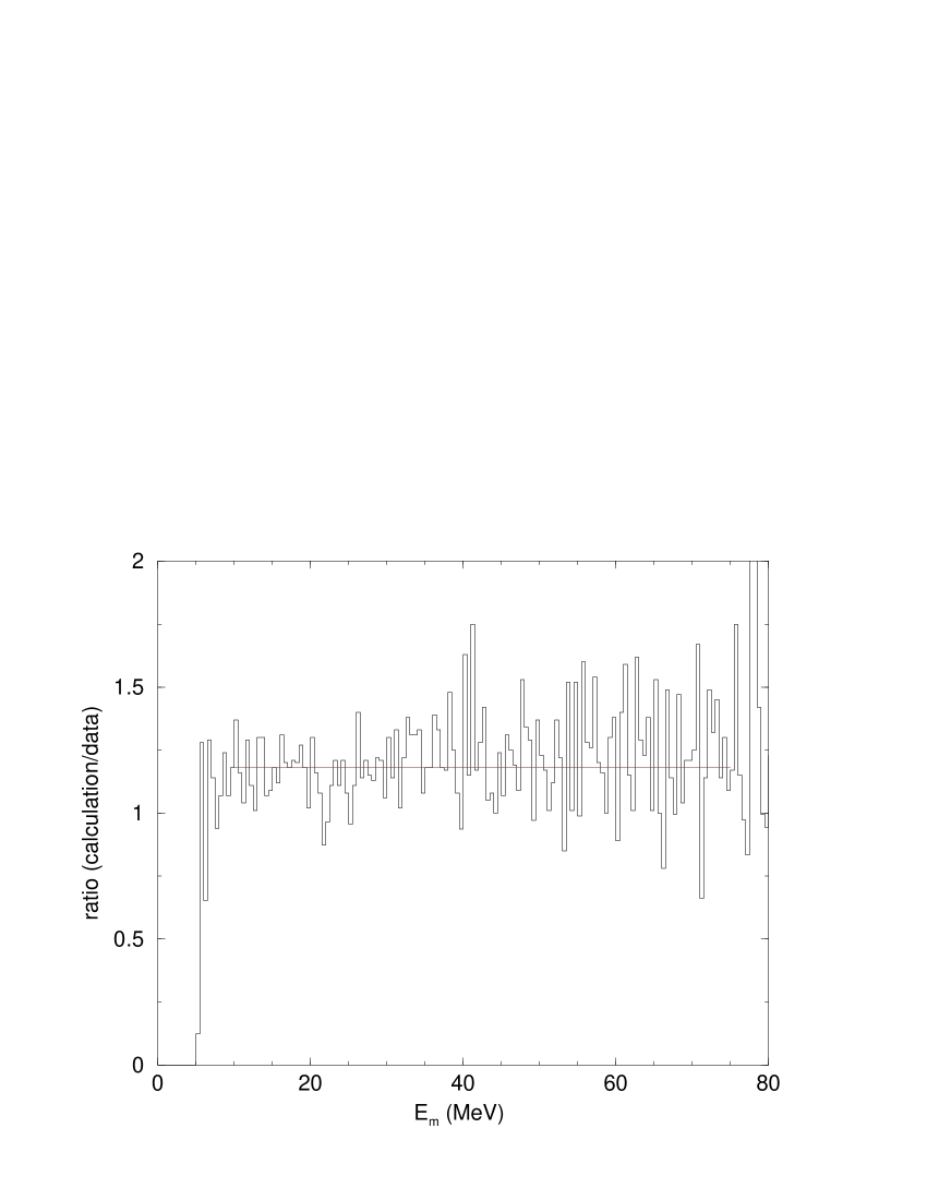
FIG. 7.: Ratio of simulated $(e,e^{\prime}p)$ spectrum (normalized by 0.84 as discussed in the text) to the experimentally measured cross section spectrum, plotted as a function of missing energy. A one-parameter fit to these data over the region $10<E_{m}<75$ MeV yields a ratio of 1.18 (shown in the figure). The bin-to-bin fluctuations in the ratio are due to the statistical uncertainties in both the cross section and the simulation. The only significant deviation from the fit is below 10 MeV, where the ratio decreases towards unity.

B Radiation Tail Correction for Multiple-Photon Processes

The Schwinger correction, which has been applied to the “unradiated” strength dominating the region of low $E_{m}$, includes the effects of multiple-photon emission and here the simulation and data agree. The tail region cross section has been derived to first order in real-photon emission, and here the simulation does not agree with the measured data. Multiple photon processes are therefore clearly indicated as a likely source of the discrepancy in the tail strength.

A rigorous derivation of a multiple-photon tail cross section is beyond the scope of this paper, but an intuitive derivation is easy to provide. In the limit that the variation in the PWIA vertex cross section is very slow, bremsstrahlung processes only redistribute strength with respect to the asymptotic kinematics. Thus if we add the “unradiated” part still residing in the peak to that residing in the tail, we should recover the original PWIA cross section $\sigma_{\mathrm{pwia}}$. $\delta_{r}$ represents the fraction of strength radiated out of the peak, to first order. Thus if the Borie-Drechsel cross section is valid in first order, its integral will also yield a fraction $\delta_{r}$ of $\sigma_{\mathrm{pwia}}$. However, the fraction remaining in the peak has been adjusted to account for higher-order radiation; the cross section here is $e^{-\delta_{r}}\sigma_{\mathrm{pwia}}$. The sum of the two is $\left(e^{-\delta_{r}}+\delta_{r}\right)\sigma_{\mathrm{pwia}}$. The factor in parentheses is differs from unity in second order. If we apply the multiplicative factor

$\displaystyle f_{\mathrm{mp}}=\frac{\left(1-e^{-\delta_{r}}\right)}{\delta_{r}}$

to the tail cross section, we recover $\sigma_{\mathrm{pwia}}$ for the sum of peak and tail cross sections in the presence of bremsstrahlung.

Note that this discussion only concerns the real-photon part of the internal bremsstrahlung correction. The external bremsstrahlung distribution described above is an energy-loss distribution which includes the higher-order contributions, thus they do not need to be considered here.

C Simulation including multi-photon tail correction

The simulation was repeated including the multi-photon tail correction, but otherwise identical (including the scaling factor 0.84). The results are presented in Figs. 8 and 9.

FIG. 8.: Differential cross sections measured in the Mainz experiment (histogram) and computed by the simulation program (solid line). The experimental data have not been corrected for bremsstrahlung effects. The full multi-photon tail correction $f_{\mathrm{mp}}$ has been used.

The reproduction of the shape of the tail is still excellent, which is not surprising. For the chosen kinematics, $\delta_{r}$ has an average value of 0.46, with a $1\sigma$ deviation of only 0.8% across the physical acceptance — $f_{\mathrm{mp}}$ is essentially a multiplicative constant for the entire tail. However, the simulation now reproduces the strength of the tail to the same level of accuracy as for the peak region. These excellent results provide unambiguous proof that multiple-photon processes are important in the radiation tail, and also that our proposed correction factor is valid at the few percent level (at least in the kinematical regime studied here).

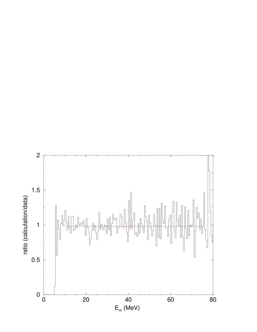
FIG. 9.: Ratio of simulated $(e,e^{\prime}p)$ spectrum (including the full tail correction and normalized by 0.84 as discussed in the text) to the experimentally measured cross section spectrum, plotted as a function of missing energy. A one-parameter fit to these data over the region $10<E_{m}<75$ MeV yields a ratio of 0.98 (shown in the figure). The bin-to-bin fluctuations in the ratio are due to the statistical uncertainties in both the cross section and the simulation.

Finally, we show in Fig. 10 a similar comparison of experimental and simulated cross-section spectra, except here we consider an expanded range of $p_{m}$. This check was made to ensure that our agreement had not been fine-tuned for only the small region of $p_{m}$ we had been considering. The corresponding ratio plot is very similar to Fig. 9, with the one-parameter fit yielding a ratio 0.976. The same simulation produced both Figs. 8 and 10; the only difference was a change in the $p_{m}$ condition specified in the histogram-sorting program.

FIG. 10.: Comparison of experimental data to simulation (including tail correction). The plot shown is identical to that of Fig. 8 except for the current plot, events (both experimental and simulated) with missing momenta $30\leq p_{m}\leq 100$ MeV/c are included. The bin size has been reduced to 0.25 MeV due to the much better statistical precision of these data.

D Decomposition of Cross Section

It is instructive to separate this cross section calculation into its components. This is a luxury that nature does not afford the experimenter. One such decomposition is shown in Fig. 11. Recall that what one usually wants to measure is the cross section with the radiation tail removed. This corresponds to the dotted line in Fig. 11, which is the simulation result for continuum breakup ${}^{3}\mbox{He}(e,e^{\prime}p)np$ with bremsstrahlung turned off. The dashed curve shows the simulation for ${}^{3}\mbox{He}(e,e^{\prime}p)d$ only, but including the full bremsstrahlung tail. The solid curve is the total simulation result as shown in Fig. 8.

FIG. 11.: Decomposition of simulated $(e,e^{\prime}p)$ cross section. The solid curve gives the final result for the cross section including the entire spectral function and all radiative processes. The long-dashed curve only includes the two-body ${}^{3}\mbox{He}(e,e^{\prime}p)d$ part of the spectral function, along with both classes of bremsstrahlung. The dotted curve includes only the continuum ${}^{3}\mbox{He}(e,e^{\prime}p)np$ part of the spectral function, and the bremsstrahlung effects are not included. When measuring in the continuum, the dotted curve is what one attempts to extract, and the long-dashed curve is physical background which must be removed by a radiative-correction procedure.

It is immediately apparent from the figure that there is no hope of making a significant measurement for missing energies much above 15 MeV — statistical fluctuations associated with the tail subtraction procedure will render such a measurement insignificant. Most of the observed cross section for $E_{m}>20$ MeV is due to ${}^{3}\mbox{He}(e,e^{\prime}p)d$ reactions residing in the radiation tail. A new experiment, made in a kinematical regime that does not result in the generation of such a strong radiation tail, will be required to make a statistically-significant measurement of the cross section in this region.

We expect simulations such as that described here will become a standard tool in the planning of experiments at large missing energies, since one would clearly like to avoid performing an experiment in kinematical regimes in which the radiation tail is stronger than the cross section to be measured.

IX Implications for Radiative Corrections of $(e,e^{\prime}p)$ Data

We stated in the introduction that this work was begun in an effort to understand problems encountered when applying radiative corrections to the ${}^{3}\mbox{He}(e,e^{\prime}p)$ data discussed here. Fig. 12 (from Ref. [1]) illustrates the problem.

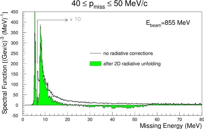
FIG. 12.: Experimental data for ${}^{3}\mbox{He}(e,e^{\prime}p)$ before and after application of radiative corrections. In this figure, the experimental spectral function is displayed, which is related to the experimental cross sections by Eq. (8).

The figure compares the measured spectral function (from the same dataset which produced Fig. 6) with the corresponding spectral function after applying radiative corrections, $i.e.$ removing the radiation tail. The tail correction procedure is essentially identical to that of [5] which was briefly described in Sec. IV. For $E_{m}>25$ MeV, the corrected spectral function is negative, clearly indicating a deficiency.

In this case, the defect can not be obviously traced to multiple-photon emission, since the tail computation is based on the distribution of the exponential form of the Schwinger correction in $E_{m}$. Specifically, the number of expected experimental counts inside a certain missing energy bin $E^{(0)}_{m}<E_{m}<E^{(0)}_{m}+\Delta E_{m}$ is given by

$\displaystyle N_{\mathrm{exp}}(E^{(0)}_{m},\Delta E_{m})=e^{-\delta_{r}(\Delta E_{m})}N_{0}(E^{(0)}_{m})\,\,.$

Here $N_{0}$ is the number of counts which would have been measured in the absence of bremsstrahlung, and $E^{(0)}_{m}$ is the missing energy at which the counts would have appeared in the absence of bremsstrahlung (or other processes which modify the asymptotic particle energies such as ionization energy loss). As $\Delta E_{m}$ becomes larger, the bin includes more of the radiation tail (the unradiated strength is included by definition) so that $N_{\mathrm{exp}}$ approaches $N_{0}$. The distribution of the radiation tail in $E_{m}$ is thus

$\displaystyle\frac{\partial N_{\mathrm{exp}}}{\partial E_{m}}=N_{0}\frac{\partial(e^{-\delta_{r}})}{\partial(\Delta E_{m})}\,\,.$

The factor $e^{-\delta_{r}}$ again explicitly includes the multiple-photon processes.

There are, however, several possible other reasons for the failure of the radiation-correction procedure. We discuss them in detail in the following sections.

A Incomplete Kinematic Reconstruction

The radiative-correction process is usually applied in two kinematic dimensions (see Ref. [1] for a thorough discussion). A common choice for the two dimensions is $(E_{m},p_{m})$. First, a two dimensional cross-section histogram is created with the independent variables being $E_{m}$ and $p_{m}$. Fig. 4 would be appropriate if the $z$-axis corresponded to cross section. As discussed in Sec. IV, the correction would begin at the left-hand edge of Fig. 4. For each bin in $p_{m}$ at this bin in $E_{m}$, correction factors would be applied and tails would be generated and subtracted for the bins to the right. In such a procedure, there is no information about any of the other kinematic parameters; a swath in seven-dimensional kinematic space has been reduced to a two-dimensional pixel. The most common remedy for this lack of information is to treat the entire bin as if the rest of the parameters were fixed at their central values. However, Fig. 4 shows a substantial dependence in the tail trajectories on the relative angle between ${\bf q}$ and ${\bf p}_{m}$. While both of these may vary across the detector acceptances, both are held fixed in the correction procedure. $|{\bf q}|$ is also held fixed, while we know that it varies substantially across the acceptances and causes large changes in the cross section through $\sigma_{ep}$. For example, at the kinematics corresponding to Fig. 12, $\delta(Q^{2})/\mu(Q^{2})$ (the standard deviation of $Q^{2}$ divided by the mean value) is about 7.6% for the pixel $5.5<E_{m}<5.9$ MeV, $40<p_{m}<50$ MeV/c. This leads to a 15% RMS variation of the cross section due to $\sigma_{ep}$ alone. The variation in the computed ${}^{3}\mbox{He}(e,e^{\prime}p)$ cross section is about 20%.

Procedures have been developed to perform the correction in more dimensions (e.g. four were used in Ref. [1]) but such schemes are only feasible for experiments with good statistical precision, as each additional dimension tends to reduce the statistical precision per bin by roughly an order of magnitude.

B Simplifying Assumptions About the Radiation Tail

The standard correction procedure uses a derivative of the Schwinger correction factor vs. $E_{m}$ to generate the tail distribution. However, as explained in Secs. IV and V, there are two directions this tail can take in $(E_{m},p_{m})$ space, corresponding to the two terms of the peaking approximation. The Schwinger correction gives no guidance as to how much strength resides in each tail. The standard practice is to assume [5, 12]:

• the incoming and outgoing electrons contribute independently to the tail, so one may factor $e^{-\delta}=C_{e}(\Delta E_{m})\,C_{e^{\prime}}(\Delta E_{m})$;

• the two contributions are equal, so $C_{e}=C_{e^{\prime}}=e^{-\delta/2}$.

The Borie-Drechsel formula (Eq. (16)) for the radiation tail clearly does not have these properties. Firstly, the two tails add instead of multiply. Secondly, they are not equal. Even for vanishingly small photon energies ($k_{e}$ and $k_{e^{\prime}}$), the two terms differ by the factors $\ln\left(2E_{e}/m_{e}\right)$ vs. $\ln\left(2E_{e^{\prime}}/m_{e}\right)$ (which have values 8.12 and 7.81 respectively in the kinematics studied here). As the radiated-photon energy increases, the difference between the two terms also increases; for a photon energy of 100 MeV, the incident-electron contribution is 6% larger than that of the scattered electron in the present kinematics. The difference between the tail magnitudes is mainly driven by the ratio $\omega/E_{e}$; when it is large, the tail strengths differ more. For a specific experiment planned at JLab with $\omega=834$ MeV and $E_{e}=1245$ MeV, the two tails differ by about 16% in strength.

C Comparison With Direct Tail Simulation

The radiation tail calculation presented here suffers from none of the above deficiencies.

• the tail is generated event-by-event, so for each tail evaluation, the complete kinematic information is available

• the distribution of the tail strength in this kinematic space is based on a first-order QED calculation, not on plausible assumptions.

The main deficiency of our computation is the nature of the multi-photon correction factor. It is based on arguments of probability conservation rather than on a rigorous QED calculation. This argument is however of the same type which leads to the exponentiation of $\delta_{r}$ in the standard approach. A critical review of including higher-order terms via exponentiation (including a summary of relevant literature) can be found in [16].

D An Improved Radiative Correction Procedure

The findings reported above indicate that the standard radiative correction procedure is not likely to work for cases in which the detector acceptances are relatively large (producing large variations in $Q^{2}$ for individual pixels in cross-section histograms) or in which a correction is being made over a large range in $E_{m}$ (so that the differences between the two tails becomes important). Our findings suggest an improved method for radiatively “correcting” experimental data.

The procedure would begin with a model spectral function and an accurate model of the experimental apparatus, such as has been described here. A simulation code similar to ours should be used to generate a “radiated” cross section spectrum. A comparison between the experimental and simulated histograms will indicate regions of discrepancy, and the discrepancy function can be used to modify the model spectral function. The procedure is repeated until it converges, at which point the model spectral function corresponds to the unradiated result. This procedure is independent of the PWIA if we replace the theoretical spectral function described above with the “distorted” spectral function [26]. We learned during the final stages of preparing this article that such an iterative procedure has been developed and successfully applied for an experiment in Hall C at Jefferson Lab [27].

X Further Work

It is desirable to have a more rigorous theory provide the multi-photon tail cross section. The beginnings of such an approach can be found in [4]. We encourage this group to complete and publish these results, especially since they have made some detailed evaluations of their approach in the Jefferson Lab energy domain.

It would also be interesting to reanalyze some of the older high-$E_{m}$ $(e,e^{\prime}p)$ data using the improved technique described here, since these data have been a source of controversy, given the sometimes puzzling behavior of the cross section at high missing energies. The current study indicates that some of this cross section might well be misidentified bremsstrahlung strength.

XI Conclusions

We have presented a framework for computing $(e,e^{\prime}p)$ cross sections which includes the radiation tail to first order. The computed cross sections have been compared to experimental data in such a way that effects such as acceptance averaging are correctly accounted for, allowing a direct evaluation of the radiation tail cross section calculation.

The computed tail reproduces both the shape and magnitude of the experimental spectrum perfectly within experimental errors. It was necessary to derive a correction, applied to the radiation tail, for higher-order bremsstrahlung effects before this agreement could be obtained; the original tail calculation treated bremsstrahlung only to first order.

A standard radiative correction procedure has also been applied to these data. Such a procedure is designed to move the radiation tail strength back into the originating kinematic bins. The straightforward application of this procedure (that is, without tweaking parameters to improve the agreement) results in physically unreasonable “deradiated” cross sections in the tail-dominated part of the spectrum. There are several reasons to expect such a failure. An obvious one is that this procedure collapses a complicated kinematical hypersurface (along which the cross section varies substantially) to a single point in $(E_{m,}p_{m})$. More subtle are the disturbing differences between the properties of the correction-procedure tails and those of a tail cross section rigorously computed in QED. The observed flaws in the correction procedure are not likely to affect earlier data taken at low missing energies, e.g., at NIKHEF, Bates, and Mainz. They may affect earlier high-$E_{m}$ data, and will likely be fatal for several of the $(e,e^{\prime}p)$ experiments planning to measure at large-$E_{m}$ at Jefferson Lab. Our results indicate how radiative corrections should be applied so as to avoid such problems.

The current project has yielded quantitative illustrations of the failure of the standard radiative-correction procedure for $(e,e^{\prime}p)$ experiments. We have also shown that a simulation, coupled with an accurate model for the radiative-tail cross section, can radiate the theory (instead of deradiating the data) and achieve excellent agreement with experiment in a situation where the correction procedure fails. The simulation technique described here provides a basis for iterative radiation-correction procedures for future $(e,e^{\prime}p)$ experiments.

A Other Limitations of the PWIA

In Sec. III we were careful to distinguish the spectral-function quantities $\epsilon$ and $\textstyle\rho$ from the experimentally determined values $E_{m}$ and ${\bf p}_{m}$. Even in the absence of bremsstrahlung this is necessary since the PWIA never holds completely, and is sometimes grossly violated. For such cases, $\epsilon\neq E_{m}$ and $\mathchoice{{\hbox{\boldmath$\displaystyle\rho$}}}{{\hbox{\boldmath$\textstyle\rho$}}}{{\hbox{\boldmath$\scriptstyle\rho$}}}{{\hbox{\boldmath$\scriptscriptstyle\rho$}}}\neq-{\bf p}_{m}$. Final State Interactions (FSI) between the ejected proton and the residual nucleus provide an illustrative example of how the correspondence is broken. At the photon-proton vertex of Fig. 1, the amplitude for the interaction will depend on the particular values of $\epsilon$ and $\textstyle\rho$. A subsequent interaction between the ejected proton and the residual nucleus can change both the momentum and excitation energy of the residual system, thus leading (through Eq. (2)) to values for $E_{m}$ and ${\bf p}_{m}$ different than $\epsilon$ and $\textstyle\rho$. While this point is not particularly relevant for the present work, we mention it here for completeness and because it is apparently often overlooked.

REFERENCES

- [1] R. E. J. Florizone, Ph.D. thesis, Massachusetts Institute of Technology, 1999.
- [2] R. E. J. Florizone et al., submitted to Phys. Rev. Lett.
- [3] C. de Calan, H. Navelet, and J. Picard, Nucl. Phys. B348, 47 (1991).
- [4] N. C. R. Makins, Ph.D. thesis, Massachusetts Institute of Technology, 1994.
- [5] E. N. M. Quint, Ph.D. thesis, Universiteit van Amsterdam, 1988.
- [6] S. Penner, Nuclear Structure Physics, Proceedings of the 18th Scottish Univ. Summer School in Physics (1977). This item is available by special order from the Scottish Universities Summer School Program, information available from http://www.sussp.ac.uk/ .
- [7] E. Borie and D. Drechsel, Nucl. Phys. A167, 369 (1971).
- [8] J. Schwinger, Phys. Rev. 75, 898 (1949).
- [9] L. W. Mo and Y. S. Tsai, Rev. Mod. Phys. 41, 205 (1969).
- [10] Y. S. Tsai, Rev. Mod. Phys. 46, 815 (1974).
- [11] L. Lapikás, Nucl. Phys. A553, 297c (1993).
- [12] M. W. Holtrop, Ph.D. thesis, Massachusetts Institute of Technology, 1995.
- [13] E. Jans et al., Nucl. Phys. A475, 687 (1987).
- [14] T. de Forest, Nucl. Phys. A392, 232 (1983).
- [15] G. G. Simon, Nucl. Phys. A333, 381 (1980).
- [16] L. C. Maximon, Rev. Mod. Phys. 41, 193 (1969).
- [17] Y. S. Tsai, Phys. Rev. 122, 1898 (1961).
- [18] J. A. Templon, Technical Report No. 97-002, University of Georgia Nuclear Group.
- [19] C. E. Vellidis, AEEXB: A Program for Monte Carlo Simulations of coincidence electron-scattering experiments, OOPS Collaboration Internal Report, MIT-Bates Accelerator Laboratory, 1998.
- [20] D. C. Carey, K. L. Brown, and C. Iselin, DECAY TURTLE (Trace Unlimited Rays Through Lumped Elements), A Computer Program for Simulating Charged Particle Beam Transport Systems, Including Decay Calculations, SLAC Publication SLAC-246, 1982.
- [21] J. A. Templon, Technical Report No. 98-001, University of Georgia Nuclear Group.
- [22] A. Kievsky, E. Pace, G. Salmè, and M. Viviani, Phys. Rev. C 56, 64 (1997).
- [23] G. Salmè, private communication, 1997.
- [24] W. U. Boeglin, Czech. J. Phys. 45, 295 (1995).
- [25] K. I. Blomqvist et al., Nucl. Instrum. Meth. A403, 263 (1998).
- [26] J. J. Kelly, in Advances in Nuclear Physics, edited by J. W. Negele and E. Vogt (Plenum Press, New York, 1996), Vol. 23, p. 75.
- [27] D. Dutta, Ph.D. thesis, Northwestern University, 1999.