Neutron capture of ²⁶Mg at thermonuclear energies

Abstract

The neutron capture cross section of ²⁶Mg was measured relative to the known gold cross section at thermonuclear energies using the fast cyclic activation technique. The experiment was performed at the 3.75 MV Van-de-Graaff accelerator, Forschungszentrum Karlsruhe. The experimental capture cross section is the sum of resonant and direct contributions. For the resonance at $E_{\rm{n,lab}}=220~{}{\rm{keV}}$ our new results are in disagreement with the data from Weigmann et al. An improved Maxwellian averaged capture cross section is derived from the new experimental data taking into account $s$- and $p$-wave capture and resonant contributions. The properties of so-called potential resonances which influence the $p$-wave neutron capture of ²⁶Mg are discussed in detail.

I Introduction

Neutron capture processes of neutron–rich light isotopes play an important role in astrophysical scenarios ranging from the so–called inhomogeneous Big Bang models to nucleosynthesis in stellar helium and carbon burning stages. In Inhomogeneous Big Bang Models the high neutron flux induced primordial nucleosynthesis bridges the mass 5 and mass 8 gap [1]. Subsequent neutron capture processes of neutron–rich isotopes may even lead to a primordial r–process [2, 3]. The efficiency for the production of heavy elements in such a scenario depends sensitively on the respective neutron capture rates for these light isotopes. Therefore the neutron capture cross sections have to be determined over a wide energy range up to about 1 MeV.

In massive Red Giant stars magnesium isotopes are mainly the products of hydrostatic carbon and neon burning. ²⁵Mg and ²⁶Mg have also appreciable abundances in the outer carbon layer as a result of the reactions ²²Ne($\alpha$,$\gamma$)²⁶Mg, ²²Ne($\alpha$,n)²⁵Mg, and ²⁵Mg(n,$\gamma$)²⁶Mg [4]. He–shell burning in low mass asymptotic giant branch (AGB) stars has been proposed as the site for the main component of the s–process [5, 6]. In AGB stars ²⁶Mg is likely to be made by ²²Ne($\alpha$,$\gamma$)²⁶Mg, as well as by ²⁵Mg(n,$\gamma$)²⁶Mg, by the decay of ²⁶Al, and by ²⁶Al(n,p)²⁶Mg with radioactive ²⁶Al being synthesized through the previous H–burning shell. For the above discussed stellar scenarios neutron capture rates need to be known in the energy range between about 5 and 200 keV.

The reaction rate for ²⁶Mg(n,$\gamma$)²⁷Mg that is being investigated in this work is low through its small cross section. The reaction ²⁶Mg(n,$\gamma$)²⁷Mg is of interest in stellar nucleosynthesis, because (i) ²⁶Mg is one of the most abundant isotopes in the cosmos, (ii) all Mg–isotopes show a strong deviation from the normal 1/v–behavior of their cross sections, and (iii) of the interplay between neutron production and captures for Mg–isotopes, and with the concurrential radioactive ²⁶Al.

The cross section for neutron capture processes is dominated by the nonresonant direct capture process (DC) and by contributions from single resonances which correspond to neutron unbound states in the compound nucleus (CN). For calculating the different reaction contributions we used a simple hybrid model: the nonresonant contributions were determined by using a direct capture model, the resonant contributions were based on determining the resonant Breit Wigner cross section. In the case of broad resonances additional interference terms have to be taken into account which were neglected in the present work because the relevant resonances are relatively narrow.

In this work we also discuss the effects of potential resonances in direct capture. Potential resonances are well known in nuclear processes (see Ref. [7] and references therein), but their influence in numerical direct–capture calculations has to our knowledge not been investigated before in great detail. The reaction ²⁶Mg(n,$\gamma$)²⁷Mg provides an excellent example for discussing the artifacts such resonances can produce in direct–capture calculations.

Up to now the neutron capture cross section of ²⁶Mg was measured at thermal energies in several experiments (see Refs. [8, 9, 10], and references therein). However, at thermonuclear energies only the resonance properties of four resonances in ²⁶Mg(n,$\gamma$)²⁷Mg were determined by Weigmann et al. [11], and in that work the Maxwellian averaged capture cross section $<\sigma>\,=\,<\sigma\cdot v>\,/\,v_{\rm T}$, with $v_{\rm T}=\sqrt{2k_{B}T/\mu}$, was calculated by the sum of the $s$-wave contribution (extrapolated from the thermal capture cross section assuming the usual $1/v$ law) and of the contributions from the four measured resonances. The $p$-wave contribution of the DC was neglected in that work.

In the following we will present our experimental procedure and results in Sect. II. In Sect. III we analyze our new experimental data using the DC model and we discuss the properties of so-called potential resonances, in Sect. IV we show the improved Maxwellian averaged capture cross section $<\sigma>$, and the results are discussed in Sect. V.

II Experimental Setup and Results

The experiment was performed at the 3.75 MV Van-de-Graaff accelerator of the Forschungszentrum Karlsruhe. The residual nucleus ²⁷Mg decays with a half-life of $T_{1/2}=9.458~{}{\rm{min}}$ to ²⁷Al. Two $\gamma$ rays with $E_{\gamma}=843.76~{}{\rm{keV}}$ (branching 71.8 %) and $E_{\gamma}=1014.44~{}{\rm{keV}}$ (branching 28.0 %) can be detected [12]. The decay properties of ²⁷Mg and ¹⁹⁸Au (from the neutron capture of ¹⁹⁷Au) are listed in Table I.

A Fast cyclic activation technique

For residual nuclei with short half-lives the fast cyclic activation technique was developed at the Forschungszentrum Karlsruhe [13]. In the ²⁶Mg experiment the sample is irradiated for a period $t_{\rm b}$, after this irradiation time the sample is moved to the counting position in front of a high–purity germanium (HPGe) detector (waiting time $t_{\rm{w_{1}}}$). The $\gamma$–rays following the $\beta$–decay of ²⁷Mg are detected for a time interval $t_{\rm c}$, and finally the sample is moved back to the irradiation position (waiting time $t_{\rm{w_{2}}}$). The whole cycle with duration $T=t_{\rm b}+t_{\rm{w_{1}}}+t_{\rm c}+t_{\rm{w_{2}}}$ is repeated many times to gain statistics. The ²⁶Mg(n,$\gamma$)²⁷Mg experiment was performed partly with $t_{\rm b}=49.6~{}{\rm{s}}$, $t_{\rm{w_{1}}}=0.4~{}{\rm{s}}$, $t_{\rm c}=49.6~{}{\rm{s}}$, $t_{\rm{w_{2}}}=0.4~{}{\rm{s}}$, $T=100~{}{\rm{s}}$, partly with $t_{\rm b}=119.4~{}{\rm{s}}$, $t_{\rm{w_{1}}}=0.6~{}{\rm{s}}$, $t_{\rm c}=119.4~{}{\rm{s}}$, $t_{\rm{w_{2}}}=0.6~{}{\rm{s}}$, $T=240~{}{\rm{s}}$.

The accumulated number of counts from a total of $N$ cycles, $C=\sum_{i=1}^{n}C_{i}$, where $C_{i}$, the counts of the i-th cycle, are calculated for a chosen irradiation time, $t_{\rm b}$, which is short enough compared with the fluctuations of the neutron flux, is [13]

$$C=\epsilon_{\gamma}K_{\gamma}f_{\gamma}\lambda^{-1}[1-\exp(-\lambda t_{\rm c})]\exp(-\lambda t_{\rm{w_{1}}})\frac{1-\exp(-\lambda t_{\rm b})}{1-\exp(-\lambda T)}N\sigma_{\gamma}{[1-f_{\rm b}\exp(-\lambda T)]}\sum_{i=1}^{n}\Phi_{i}$$ (1)

with

$$f_{\rm b}=\frac{\sum_{i=1}^{n}\Phi_{i}\exp[-(n-i)\lambda T]}{\sum_{i=1}^{n}\Phi_{i}}\quad.$$ (2)

The following additional quantities have been defined: $\epsilon_{\gamma}$: detection efficiency, $K_{\gamma}$: $\gamma$-ray absorption, $f_{\gamma}$: $\gamma$-ray intensity per decay, $\lambda$: decay constant, $N$: the thickness (atoms per barn) of target nuclei, $\sigma_{\gamma}$: the capture cross section, $\Phi_{i}$: the neutron flux in the i-th cycle. The quantity $f_{\rm b}$ is calculated from the registered flux history of a ⁶Li glass monitor which is mounted at a distance of 91 cm from the neutron production target. A simple n–$\gamma$ discrimination was applied to the slow output of the ⁶Li monitor: the amplitude of the neutron signal from the ⁶Li(n,$\alpha$)³H reaction is much larger than the amplitude from a typical $\gamma$ ray event that cannot deposit its full energy in the 1 mm thin ⁶Li glass scintillator.

The experimental uncertainties are reduced to a great amount by measuring the ²⁶Mg capture cross section relative to the well-known gold standard [14]. For this purpose our magnesium samples were sandwiched between two thin gold foils. Then the capture cross section of the sample $\sigma_{\gamma}^{\rm S}$ is given relative to the capture cross section of the gold reference $\sigma_{\gamma}^{\rm R}$ by:

$$\sigma_{\gamma}^{\rm S}=\sigma_{\gamma}^{\rm R}\;\frac{C^{\rm S}N^{\rm R}\epsilon_{\gamma}^{\rm R}K_{\gamma}^{\rm R}f_{\gamma}^{\rm R}\lambda^{\rm S}[1-\exp(-\lambda^{\rm R}t_{\rm c})]\exp(-\lambda^{\rm R}t_{\rm{w_{1}}})[1-\exp(-\lambda^{\rm R}t_{\rm b})][1-\exp(-\lambda^{\rm S}T)]{[1-f_{\rm b}^{\rm R}\exp(-\lambda^{\rm R}T)]}}{C^{\rm R}N^{\rm S}\epsilon_{\gamma}^{\rm S}K_{\gamma}^{\rm S}f_{\gamma}^{\rm S}\lambda^{\rm R}[1-\exp(-\lambda^{\rm S}t_{\rm c})]\exp(-\lambda^{\rm S}t_{\rm{w_{1}}})[1-\exp(-\lambda^{\rm S}t_{\rm b})][1-\exp(-\lambda^{\rm R}T)]{[1-f_{\rm b}^{\rm S}\exp(-\lambda^{\rm S}T)]}}$$ (3)

B Samples

Our samples consisted of MgO powder enriched in ²⁶Mg by 98.79 % and of metallic magnesium of natural isotopic composition. The MgO powder was pressed to two small tablets with a diameter of $d=6~{}{\rm{mm}}$ and a thickness of about 0.5 mm and 1.5 mm, respectively. The MgO tablets were put into a thin Al foil to ensure that no powder is lost during the measurements. The mass of the tablets had to be determined very carefully because the MgO powder is very hygroscopic. Therefore, the tablets were heated at $T\approx 1000^{\circ}~{}{\rm{C}}$ for several hours, and then they were weighted during the cooling phase. We removed the tablets from the oven at about $300^{\circ}~{}{\rm{C}}$. After this procedure we found that the measured weight of the tablets was stable for a few minutes, but then the weight began to increase by about 10 to 20 percent within a few hours.

As a further check we repeated one activation measurement with a sample of metallic ^natMg with the same geometric shape (diameter 6 mm, thickness 1 mm, mass 47.77 mg). The result agreed perfectly with the cross section measured with the enriched samples. This confirms that the weighting procedure worked well, that the enrichment of ²⁶Mg in the MgO samples was correct, and that the influence of degraded neutrons scattered by hydrogen in the hygroscopic MgO samples is negligible. The properties of the samples are summarized in Table II.

C Neutron production, Time-of-Flight measurements

The neutrons for the activation were generated using the ⁷Li(p,n)⁷Be reaction. We measured the capture cross section in the astrophysically relevant energy region of several keV at six different neutron energies which are obtained by different combinations of proton energy and thickness of the lithium target: ($i$) Close above the reaction threshold at $E_{\rm{p,lab}}=1881~{}{\rm{keV}}$ one obtains a quasi–Maxwellian spectrum with $k_{B}T=25~{}{\rm{keV}}$ [15] if the energy loss of the protons in the lithium layer of the target reduces the proton energy below the reaction threshold. ($ii$) Very close to the reaction threshold a narrow spectrum with $12~{}{\rm keV}\leq E_{\rm{n,lab}}\leq 52~{}{\rm keV}$ was obtained. Note that in these cases ($i$) and ($ii$) the neutron energy spectrum is independent of the thickness of the lithium layer. We used a lithium layer of 30 $\mu$m which is by far thick enough for that purpose. ($iii$) Using four different higher proton energies we obtained four different neutron energy spectra with higher neutron energies and an energy width of about 20–50 keV. Now the energy width depends sensitively on the thickness of the lithium layer which was about 2.6 $\mu$m in our experiment. The thicknesses of the different thin lithium targets were determined by two independent methods: first during the evaporation of the metallic lithium layer and second from the width of the time-of-flight spectra (see below). Both methods give the same results within an uncertainty of about 10%.

For the activation runs beam currents in the order of 80 to 100 $\mu$A were used. Because of the electric power of the proton beam of about $P\approx 2~{}{\rm{MV}}\cdot 100~{}{\rm{\mu A}}\approx 200~{}{\rm{W}}$ the copper backing of the thin lithium layer was water-cooled, and the temperature of the copper backing remained below 85^oC during the whole experiment.

The neutron energy spectra were controlled by time-of-flight (TOF) measurements using the pulsed beam which is available from the Van-de-Graaff accelerator. Typically the repetition frequency is 1 MHz, and the pulse width is about 10 ns. The beam current in the pulsed mode was about 1 to 4 $\mu$A. The neutrons were detected in the ⁶Li glass monitor, and the TOF of the neutrons was measured between the fast timing output from the ⁶Li monitor (start) and the delayed pickup signal from the pulsed beam (stop). Especially at energies close to the resonances in the ²⁶Mg(n,$\gamma$)²⁷Mg reaction the energy of the neutrons has to be determined very accurately. A typical TOF spectrum at $\vartheta_{\rm{lab}}=0^{\circ}$ is shown in Fig. 1.

The result of our experiment is an average capture cross section

$$\bar{\sigma}=\int\sigma(E_{\rm{n,lab}})\Phi(E_{\rm{n,lab}})dE_{\rm{n,lab}}$$ (4)

where the neutron energy distribution $\Phi(E_{\rm{n,lab}})$ is normalized to 1:

$$\int\Phi(E_{\rm{n,lab}})dE_{\rm{n,lab}}=1$$ (5)

The neutron energy distribution $\Phi(E_{\rm{n,lab}})$ was calculated from the measured TOF distribution $\Phi(T)$ by the relation $\Phi(T)dT=\Phi(E_{\rm{n,lab}})dE_{\rm{n,lab}}$. Additionally several facts have to be taken into account: ($i$) the angular dependence of the ⁷Li(p,n)⁷Be reaction cross section which was measured at several angles using the ⁶Li monitor [16], ($ii$) the geometry of the neutron production target and the sample, ($iii$) the energy loss of the protons in the lithium layer with a thickness $d=2600~{}{\rm{nm}}\pm 10\%$ [17], ($iv$) the low-energy tail of the neutron energies in the TOF spectrum (see Fig. 1). ($iii$) and ($iv$) are relevant only for the measurements at higher neutron energies. The neutron energy distribution with $\bar{E}_{\rm{n,lab}}=208.3~{}{\rm{keV}}$ is shown in Fig. 2. It has to be pointed out that it is difficult to measure the effective neutron energy distribution $\Phi(E_{\rm{n,lab}})$ directly because of the extended lithium target and the extended sample. However, all ingredients ($i$)–($iv$) for the calculation of $\Phi(E_{\rm{n,lab}})$ were determined experimentally, and so the uncertainties of the calculation are small.

D $\gamma$ ray detection

The $\gamma$ rays from the decay of ²⁷Mg and ¹⁹⁸Au were detected using a high purity germanium (HPGe) detector with a relative efficiency of 60 % (compared to a 3” x 3” NaI detector). The energy-dependent efficiency of the HPGe detector was calculated using the detector simulation program GEANT [18]. The simulation calculation was controlled by an experimental determination of the efficiency with several radioactive calibration sources. The results for the relative efficiencies are

$$\frac{\epsilon_{\gamma}(411.80~{}{\rm{keV}})}{\epsilon_{\gamma}(843.76~{}{\rm{keV}})}=1.752\pm 2\% \frac{\epsilon_{\gamma}(411.80~{}{\rm{keV}})}{\epsilon_{\gamma}(1014.44~{}{\rm{keV}})}=2.016\pm 2\%\,\,\,\mbox{for}\,\,\,d=30~{}{\rm{mm}}$$ and (6)

$$\frac{\epsilon_{\gamma}(411.80~{}{\rm{keV}})}{\epsilon_{\gamma}(843.76~{}{\rm{keV}})}=1.746\pm 2\% \frac{\epsilon_{\gamma}(411.80~{}{\rm{keV}})}{\epsilon_{\gamma}(1014.44~{}{\rm{keV}})}=2.007\pm 2\%\,\,\,\mbox{for}\,\,\,d=35~{}{\rm{mm}}$$ and (7)

for the close geometry used in our experiment (the distance between sample and detector was 30 mm for the $k_{B}T=25~{}{\rm{keV}}$ runs and for the run very close above the threshold, and 35 mm for the other runs). Additionally, the $\gamma$–ray absorption in the sample and in the gold foils was calculated using the cross section tables provided by National Nuclear Data Center, Brookhaven National Laboratory, via WWW, and based on Ref. [19]. This small correction is in the order of a few %. A typical spectrum from the HPGe detector is shown in Fig. 3.

E Experimental Results

The new experimental data are listed in Table III, and they are compared to a DC calculation (see Sect. III) in Fig. 4. Two of the four known resonances at $E_{\rm{n,lab}}=68.7~{}{\rm{keV}}$, 220 keV, 427 keV, and 432 keV [11] have influence on our measured cross sections at $k_{B}T=25~{}{\rm{keV}}$ (resonance at 68.7 keV) and at $E_{\rm n,lab}=178~{}{\rm{keV}}$ and $208~{}{\rm{keV}}$ (resonance at 220 keV). The two resonances above 400 keV do not influence our measurement because they are narrow ($\Gamma\leq 2~{}{\rm{keV}}$) [11].

The influence of a narrow resonance at the energy $E_{\rm{res}}$ on the measured capture cross section can be calculated by

$$\bar{\sigma}_{\rm{res}}=\int\sigma_{\rm{BW}}(E_{\rm{c.m.}})\Phi(E_{\rm{c.m.}})dE_{\rm{c.m.}}\approx\Phi(E^{\rm{res}}_{\rm{n,lab}})\;\frac{A_{P}+A_{T}}{A_{T}}\;2\pi\;\frac{\pi}{{(k^{\rm{res}}_{\rm{c.m.}})}^{2}}\;(\omega\gamma)$$ (8)

where $\sigma_{\rm{BW}}(E_{\rm{c.m.}})$ is the Breit-Wigner shaped capture cross section in the resonance, $\Phi(E)$ the neutron energy distribution, $k^{\rm{res}}_{\rm{c.m.}}$ the wave number at the resonance energy $E_{\rm{res}}=\hbar^{2}(k^{\rm{res}}_{\rm{c.m.}})^{2}/2\mu$ in the center-of-mass system, and $\omega\gamma$ is the resonance strength.

The resonance strength of the $E_{\rm{n,lab}}=220~{}{\rm{keV}}$ resonance was measured by Weigmann et al. [11]: $\omega\gamma=3.75\pm 0.16~{}{\rm{eV}}$. This resonance gave the dominating contribution to the capture cross section for the neutron energy spectrum $\Phi(E_{\rm{n,lab}})$ shown in Fig. 2 (corresponding to $E^{0}_{\rm{p,lab}}=2003~{}{\rm{keV}}$). ¿From Eq. 8 one obtains $\bar{\sigma}_{\rm{res}}=1.78\pm 0.27~{}{\rm{mb}}$. In contradiction to that result our measured capture cross section is only $\sigma=0.735\pm 0.040~{}{\rm{mb}}$ as shown in Fig. 4!

Our method for measuring neutron capture cross sections is mainly tailored for non-resonant capture. Nevertheless, our experimental result definitely excludes the result of Weigmann et al. [11] for the resonance at 220 keV. To estimate the uncertainties of our calculated $\Phi(E_{\rm{n,lab}})$ we calculated energy distributions $\Phi(E_{\rm{n,lab}})$ also at proton energies $E_{\rm{p,lab}}=E^{0}_{\rm{p,lab}}\pm 2~{}{\rm{keV}}$ which is much larger than the uncertainty of the accelerator calibration which was confirmed by the TOF measurements. These results for $E_{\rm{p,lab}}=E^{0}_{\rm{p,lab}}\pm 2~{}{\rm{keV}}$ are also shown in Fig. 2 as dashed lines. The resulting uncertainties for $\Phi(E_{\rm lab}=220~{}{\rm{keV}})$ and $\bar{\sigma}_{\rm{res}}$ are about 15%.

If one subtracts the expected non-resonant DC contribution $\sigma_{\rm DC}=0.095\pm 0.010~{}{\rm{mb}}$ (see also Sects. III A and IV) from our measured capture cross section at $E_{\rm{n,lab}}=208.3~{}{\rm{keV}}$ ($E_{\rm{c.m.}}=200.3~{}{\rm{keV}}$) we obtain a resonant contribution of $\bar{\sigma}=0.64\pm 0.05~{}{\rm{mb}}$, which is a factor of about 2.8 lower than the result from Weigmann et al. [11]. Therefore, we obtain a resonance strength of $\omega\gamma=1.34\pm 0.24~{}{\rm{eV}}$ for the $E_{\rm{n,lab}}=220~{}{\rm{keV}}$ resonance. Interference effects between the DC and the $E_{\rm{n,lab}}=220~{}{\rm{keV}}$ resonance can be neglected because the total width of this resonance is relatively small: $\Gamma=0.44\pm 0.07~{}{\rm{keV}}$ [11].

A similar analysis of the 68.7 keV resonance has relatively large uncertainties because only the tail of the neutron energy spectrum with $k_{B}T=25~{}{\rm{keV}}$ overlaps with this relatively weak resonance ($\omega\gamma=73\pm 20~{}{\rm{meV}}$ from Ref. [11], at least more than one order of magnitude smaller than the $E_{\rm{n,lab}}=220~{}{\rm{keV}}$ resonance), and the dominating contributions to this data point at $k_{B}T=25~{}{\rm{keV}}$ come from $s$- and $p$-wave capture.

III Theoretical Analysis

A Direct capture model and folding potentials

The theoretical analysis was performed within the Direct Capture (DC) model. The DC cross section is given by [20, 21]

$$\sigma_{\gamma i}^{{\rm DC}}=\int{\rm d}\Omega\,2\,\left(\frac{e^{2}}{\hbar\,{\rm c}}\right)\left(\frac{\mu{\rm c}^{2}}{\hbar\,{\rm c}}\right)\left(\frac{k_{\gamma}}{k_{a}}\right)^{3}\frac{1}{2\,I_{A}+1}\,\frac{1}{2\,S_{a}+1}\sum_{M_{A}\,M_{a}\,M_{B},\,\pi_{\gamma}}\mid T_{M_{A}\,M_{a}\,M_{B},\,\pi_{\gamma}}\mid^{2}\quad.$$ (9)

The quantities $I_{A}$, $I_{B}$ and $S_{a}$ ($M_{A},M_{B}$ and $M_{a}$) are the spins (magnetic quantum numbers) of the target nucleus $A$, residual nucleus $B$ and projectile $a$, respectively. The reduced mass in the entrance channel is given by $\mu$. The polarization $\pi_{\gamma}$ of the electromagnetic radiation can be $\pm 1$. The wave number in the entrance channel and for the emitted radiation is given by $k_{a}$ and $k_{\gamma}$, respectively. The transition matrices $T=T^{\rm E1}+T^{\rm E2}+T^{\rm M1}$ depend on the overlap integrals

$$I^{{\rm E}{\cal L}/{\rm M}{\cal L}}_{l_{b}\,j_{b}\,I_{B};l_{a}\,j_{a}}=\int\,{\rm d}r\,u_{l_{b}\,j_{b}\,I_{B}}(r){\cal O}^{{\rm E}{\cal L}/{\rm M}{\cal L}}(r)\,\chi_{l_{a}\,j_{a}}(r)\quad$$ (10)

The radial part of the bound state wave function in the exit channel and the scattering wave function in the entrance channel is given by $u_{l_{b}\,j_{b}\,I_{B}}(r)$ and $\chi_{l_{a}\,j_{a}}(r)$, respectively. The radial parts of the electromagnetic multipole operators are well-known. The calculation of the DC cross sections has been performed using the code TEDCA [22].

For the calculation of the scattering wave function $\chi(r)$ and the bound state wave function $u(r)$ we used systematic folding potentials:

$$V(R)=\lambda\,V_{\rm F}(R)=\lambda\,\int\int\rho_{a}({\bf r}_{1})\rho_{A}({\bf r}_{2})\,v_{\rm eff}\,(E,\rho_{a},\rho_{A},s)\,{\rm d}{\bf r}_{1}{\rm d}{\bf r}_{2}$$ (11)

with $\lambda$ being a potential strength parameter close to unity, and $s=|{\bf R}+{\bf r}_{2}-{\bf r}_{1}|$, where $R$ is the separation of the centers of mass of the projectile and the target nucleus. The density of ²⁶Mg has been derived from the measured charge distribution [23], and the effective nucleon-nucleon interaction $v_{\rm eff}$ has been taken in the DDM3Y parametrization [24]. The resulting folding potential has a volume integral per interacting nucleon pair $J_{R}=500.41\,{\rm{MeV\,fm^{3}}}$ ($\lambda=1$) and an rms-radius $r_{\rm rms}=3.676\,{\rm{fm}}$. Details about the folding procedure can be found for instance in [25], the folding potential has been calculated by using the code DFOLD [26]. The imaginary part of the potential is very small because of the small flux into reaction channels and can be neglected in our case. This fact will be discussed in Sect. III D. The potential strength parameter $\lambda$ can be adjusted either to the binding energy $E_{B}$ (bound state wave function) or to the scattering length ($s$-wave scattering at thermal energies).

The Pauli principle was taken into account for the bound state wave functions by the condition

$$Q=2N+L$$ (12)

where $Q$, $N$, and $L$ are the number of oscillator quanta, nodes in the wave function, and angular momentum number. For even-parity states one has to take $Q=2$ in the $sd$ shell, and for odd-parity states $Q=3$. The parameters $\lambda$ for several bound state wave functions are listed in Table IV. Note that the $\lambda$ values do not differ more than 30% from unity for all bound states ($\lambda\approx 0.9$ for $Q=2$ states with positive parity, $\lambda\approx 1.25$ for $Q=3$ states with negative parity).

The total capture cross section is given by the sum over all DC cross sections for each final state $i$, multiplied by the spectroscopic factor $C^{2}S$ which is a measure for the probability of finding ²⁷Mg in a (²⁶Mg $\otimes$ n) single-particle configuration

$$\sigma_{\gamma}=\sum_{i}C^{2}_{i}S_{i}\,\sigma_{\gamma i}^{\rm{DC}}\quad.$$ (13)

For the ²⁶Mg(n,$\gamma$)²⁷Mg reaction one has to take into account all final states below the neutron threshold of ²⁷Mg. However, in practice only E1 transitions to final states with large spectroscopic factors are relevant in the keV energy region. Additionally, at thermal energies M1 and E2 transitions contribute to about 17% to the thermal capture cross section [8, 9].

B Spectroscopic factors

For the theoretical prediction of the neutron capture cross section the knowledge of the spectroscopic factors (SF) is essential. These SF have been determined from the DWBA analysis of different transfer reactions like e.g. ²⁶Mg(d,p)²⁷Mg. Unfortunately, the experimental SF from the different experiments only agree within a factor of 2 (although these experiments claim uncertainties in the order of 10–20%). Additionally, SF from theoretical shell model calculations are in average roughly a factor of 2 smaller than the experimental SF. These discrepancies are listed in Table IV.

To reduce these uncertainties the following procedure was applied. At thermal energies SF can be determined with high accuracy from the ratio of the experimental capture cross section to the calculated DC cross section. The DC cross section can be calculated with small uncertainties because the uncertainties in the calculation of the scattering wave function can be minimized by adjusting the potential strength (parameter $\lambda$) to the neutron scattering length [34]. In the case of ²⁶Mg the scattering lengths $b_{\rm bound}=4.89\pm 0.15~{}{\rm{fm}}$ [36] and $b_{\rm free}=(b_{\rm bound}-Z\;b_{\rm{ne}})\;A/(A+1)=4.725\pm 0.15~{}{\rm{fm}}$ lead to $\lambda=0.9694\pm 0.024$. Using this value for $\lambda$ we obtain for the two dominating E1 transitions at thermal energies: $C^{2}S(3/2^{-},3560~{}{\rm{keV}})=0.360\pm 0.054$ and $C^{2}S(1/2^{-},4827~{}{\rm{keV}})=0.260\pm 0.039$. The calculation includes the uncertainties of the potential strength parameter $\lambda$, of the thermal capture cross section ($\sigma_{\rm{thermal}}=39.0\pm 0.8~{}{\rm{mb}}$ [8]), and of the branching of the thermal capture [8, 9].

The result for the SF is in average 14.1% smaller than the result of Meurders et al. [27] obtained from (d,p) measurements for the two odd-parity levels for which the SF can be determined accurately as described above. Therefore, we renormalized the experimental SF from Ref. [27] by the factor $0.852\pm 0.091$. The experimental data of Ref. [27] were used because only in that experiment all relevant levels were analyzed. The result for the DC cross section is compared to the experimental results in Fig. 4. One can clearly see the transition from the $1/v$-behavior ($s$-wave capture) to the $v$-behavior ($p$-wave capture) at $E\approx 20~{}{\rm{keV}}$. This transition is typical especially for neutron-rich nuclei in the $sd$ shell with many bound states with even parity and large spectroscopic factors.

The overall agreement between the experimental data points which are not affected by the known resonances and the DC calculation is quite good. However, our DC calculation overestimates the $p$-wave capture. There are two possible explanations: (i) the spectroscopic factors of the final states with even parity (which cannot be determined by the procedure described above) are too large, (ii) the optical potential for the $p$-wave differs slightly from the $s$-wave potential.

C Potential resonances

In the following our discussion is restricted to folding potentials with one free parameter $\lambda$. The same arguments also hold for Saxon-Woods or other potentials, but in many cases the discussion may be more complicated because the larger number of parameters of the Saxon-Woods potential.

The real part of the optical potential for the incoming $p$-wave was assumed to be identical to the $s$-wave potential which was adjusted to the neutron scattering length at thermal energies. However, a weak dependence (in the order of about 10–20%) of the optical potential on the parity and/or the angular momentum of the partial wave was found in many systems (see e.g. Ref. [37]). This weak energy dependence has important consequences for the calculation of the neutron capture cross section of ²⁶Mg, because the ²⁶Mg-n potential shows a so-called potential resonance for the $p$-wave close to the astrophysically relevant energy region. This fact leads to a very sensitive dependence of the capture cross section on the potential strength (i.e. the strength parameter $\lambda$). In Fig. 5 we show the dependence of the capture cross section on the potential strength parameter $\lambda$. Changing $\lambda$ from 0.8 to about 1.0 does not change the qualitative shape of the cross section curve, but the absolute value changes by a factor of 4.5 at 1 MeV. For $\lambda>1.0$ the resonant behavior becomes more and more visible, and for $\lambda=1.10$ the resonance disappears below the threshold and leads to a bound state at $E_{B}=-135.3~{}{\rm{keV}}$.

Such potential resonances are characterized by a large width because the simple two-body potential model assumes full single-particle strength for such resonances. For very broad resonances ($\Gamma\approx E$) it is difficult to give precise numbers for the position and the width of a resonance (see e.g. the discussion in Ref. [38]). To avoid such problems of definition we show the p-wave phase shift $\delta_{l=1}(E)$ for several parameters $\lambda$ in Fig. 6, and we define the energy of the resonance as the maximum slope of the phase shift, and the width is given by the slope at that energy: $\Gamma=2\;[(d\delta_{l=1}(E)/dE)|_{E=E_{\rm{res}}}]^{-1}$. The resulting values for $E_{\rm{res}}$, $\Gamma$, and the phase shift $\delta_{l=1}(E_{\rm{res}})$ are listed in Table V.

For a proper adjustment of the $p$-wave potential strength the knowledge of the experimental scattering phase shifts is desirable. However, to our knowledge these phase shifts have not been measured. Nevertheless, there is an experimental hint that such a potential resonance is not only an artifact of the theory, but exists in nature: a broad structure was observed in a measurement of the total ²⁶Mg–n cross section at about $E\approx 300~{}{\rm{keV}}$ [36]. At that energy our potential model predicts a width of several hundred keV.

In general, several potential resonances have been proved experimentally. A typical example is the first $3^{+}$ state in ⁶Li which can be found as a resonance in the ²H($\alpha$,$\gamma$)⁶Li capture reaction [39]. Because of the almost pure single-particle structure of ⁶Li = ²H $\otimes$ $\alpha$ the properties of this resonance can be predicted by the potential model. For heavier nuclei an almost pure single-particle structure cannot be expected but there still exist broad resonances with a relatively strong single-particle component. This leads to an overestimation of the width because the simple two-body potential model assumes full single-particle structure for potential resonances. As a consequence, the potential model is not able any more to predict the properties of such resonances with high accuracy; only if the spectroscopic factor of such a resonance is known, the width can be calculated using the relation

$${\Gamma_{\rm{exp}}}=C^{2}S\,{\Gamma_{\rm{s.p.}}}$$ (14)

where $\Gamma_{\rm{s.p.}}$ is the width calculated from the potential model. Furthermore, the strength of the theoretical single-particle resonance is fragmented into several states which can be identified experimentally. This can already be seen from the fact that the two bound $p$-wave states which dominate the thermal capture cross section of ²⁶Mg(n,$\gamma$)²⁷Mg have SF in the order of about 0.2 to 0.4.

It has to be pointed out that the so-called “non-resonant” energy region can be calculated by the simple potential model only if the potential is carefully adjusted because the potential model always contains potential resonances, and as one can see from Figs. 5 and 6, there is no clear definition for “resonant” or “non-resonant”. A wrong adjustment may lead to ($i$) an overestimation of the capture cross section if the potential contains a single-particle resonance which does not exist in the experiment, and ($ii$) an underestimation of the capture cross section if the adjustment neglects strong (and broad) single-particle resonances.

The success of many previous calculations using the DC model, which seems to be in contradiction to the above statements, can be explained by two facts: ($i$) in several cases the influence of potential resonances is small in the energy region which was analyzed in the calculation (this is especially the case when the main contribution for the DC transition comes from regions far outside the nucleus, see e.g. Refs. [40] or [41]), ($ii$) even wrong DC calculations can be corrected using adjustable spectroscopic factors (uncertainties in the order of a factor of 2 are realistic, see Sect. III B!).

¿From this point of view the rough agreement of the calculated DC cross section with the experimental results is already somewhat surprising because the range of the capture cross section (see Fig. 5) covers five orders of magnitude when the potential strength changes by only $\pm 15\%$ from about 0.95 (determined from the $s$-wave scattering) down to 0.8 and up to 1.1. Such a dramatic behavior of the so-called “non-resonant” direct capture can appear in any DC calculation. To the best of our knowledge, these facts were not completely discussed in all the previous papers dealing with DC. In conclusion, we point out that the calculation of the DC has to be done with great care for each nucleus because otherwise deviations between the predicted and the experimental capture cross section not only by a factor of two, but even by orders of magnitude can appear, and both overestimations and underestimations of the experimental cross sections are possible!

D The imaginary part of the optical potential

As pointed out by Lane and Mughabghab [42], the capture amplitude has to be derived from the full optical potential, i.e. real and imaginary part (see also Eq. 10). However, in the case of ²⁶Mg(n,$\gamma$)²⁷Mg the imaginary part of the optical potential can be neglected for the following reasons. The only open inelastic channel is neutron capture. Then the capture cross section $\sigma_{\gamma}$ is directly related to the reflexion coefficient $\eta_{l}$ by:

$$\sigma_{\gamma}=\frac{\pi}{{(k_{\rm{c.m.}})}^{2}}\sum_{l}(2l+1)(1-\eta_{l}^{2})~{}.$$ (15)

Using the real folding potential with $\lambda=0.9694$ (from Sect. III B), an imaginary Saxon-Woods potential with depth $W_{0}$, reduced radius $R_{0}=1.3~{}{\rm{fm}}$ ($R=R_{0}\cdot A_{T}^{1/3}$), diffuseness $a=0.65~{}{\rm{fm}}$, and the experimentally determined values of $\sigma_{\gamma}$, one obtains a depth of the imaginary part in the order of $W_{0}\approx 100~{}{\rm{eV}}$ for the optical $s$- and $p$-wave potential. This very weak imaginary part does not significantly influence the calculated DC cross section.

A significant reduction of the DC cross section is only obtained when $W_{0}$ is increased by more than three orders of magnitude. This means that the calculations of the DC cross section in Fig. 5 are practically not influenced by the imaginary part of the potential. Only potential resonances with very huge capture cross sections (with $\lambda\approx 1.08$) will be damped slightly by the imaginary part of the potential.

IV Astrophysical reaction rates

The astrophysical reaction rate $N_{A}<\sigma\cdot v>$ can easily be derived from the Maxwellian averaged capture cross section $<\sigma>\,=\,<\sigma\cdot v>\,/\,v_{\rm T}$. The Maxwellian averaged cross section of the reaction ²⁶Mg(n,$\gamma$)²⁷Mg was calculated from the following three ingredients. First, the thermal $s$-wave capture taken from Ref. [36] was extrapolated to the thermonuclear energy region using the well-known $1/v$ law. This $1/v$ behavior is reproduced by the DC calculations. Therefore, the uncertainty of the $s$-wave contribution is below 5%. Second, the $p$-wave capture cross section which dominates at thermonuclear energies is roughly proportional to the velocity $v$:

$$\sigma=C\cdot\sqrt{E}.$$ (16)

The constant $C$ was determined from the experimental data: $C=180\pm 30~{}\rm{\mu b/\sqrt{MeV}}$. Because only three experimental cross section data are not influenced by resonances, and because one has to subtract the $s$-wave contribution from the experimental capture cross section, we estimate an uncertainty of less than 20% for the $p$-wave contribution. Note that the the $p$-wave contribution of the DC for the data point at $E_{\rm{n,lab}}=208.3~{}{\rm{keV}}$ was also taken from Eq. 16, and the $s$- and $p$-wave contribution were subtracted to determine the resonance strength of the $E_{\rm{n,lab}}=220~{}{\rm{keV}}$ resonance (see Sect. II E). Third, the resonance contributions were reduced by a factor of 2.8 compared to Ref. [11] (see discussion in Sect. II E). This factor was only determined for the $E_{\rm{n,lab}}=220~{}{\rm{keV}}$ resonance, and the uncertainty of the sum of the resonant contributions is roughly a factor of 2.

Finally, this leads to a Maxwellian averaged capture cross section $<\sigma>$ as shown in Fig. 7. At low energies ($k_{B}T<10~{}{\rm{keV}}$) $s$-wave capture is dominating, and from about $k_{B}T\approx 20~{}{\rm{keV}}$ the $p$-wave capture exceeds the $s$-wave contribution. The resonances become dominant at higher energies ($k_{B}T\approx 50~{}{\rm{keV}}$). By accident, our result is relatively close to that of Ref. [11]: the sum of our measured $p$-wave capture and the by a factor of 2.8 reduced resonant contributions is somewhat larger at $k_{B}T<30~{}{\rm{keV}}$ than the calculation of Ref. [11] which neglected the $p$-wave contribution, and at higher energies ($k_{B}T>40~{}{\rm{keV}}$) the result of Ref. [11] is higher than our new result due to the overestimation of the resonance strengths in that work.

V Summary and conclusion

There are three main results of this work: ($i$) the DC cross section of the reaction ²⁶Mg(n,$\gamma$)²⁷Mg was measured for the first time between the known resonances at $E_{\rm{n,lab}}=68.7~{}{\rm{keV}}$ and $E_{\rm{n,lab}}=220~{}{\rm{keV}}$ [11], ($ii$) the properties of potential resonances are discussed in detail for the $p$-wave capture of ²⁶Mg(n,$\gamma$)²⁷Mg, and ($iii$) the resonance strength of the $E_{\rm{n,lab}}=220~{}{\rm{keV}}$ resonance was determined to be $\omega\gamma=1.34\pm 0.24~{}{\rm{eV}}$ by a careful analysis of the neutron energy spectrum $\Phi(E_{\rm{n,lab}})$. This last result is in clear contradiction to the results of Ref. [11]. Unfortunately, in Ref. [11] the experimental information on the capture measurements is very limited, but it is stated in that work that the enriched ²⁶Mg- and ²⁵Mg-samples were analyzed in the same way. This fact makes the experimental results of Ref. [11] for the capture reaction ²⁵Mg(n,$\gamma$)²⁶Mg at least questionable. A strongly reduced ²⁵Mg(n,$\gamma$)²⁶Mg reaction rate might have influence on the $s$-process nucleosynthesis because of the role of ²⁵Mg as neutron poison. In this paper we do not want to speculate about astrophysical consequences of such a reduced reaction rate; instead, we think that primarily a new measurement of the resonance properties of ²⁵Mg is necessary to obtain reliable reaction rates. Unfortunately, the reaction ²⁵Mg(n,$\gamma$)²⁶Mg cannot be analyzed using our activation technique because the residual nucleus ²⁶Mg is stable.

TABLE I.: Decay properties of the residual nuclei ²⁷Mg and ¹⁹⁸Au.

Residual	$T_{1/2}$	$E_{\gamma}$	Intensity per decay
nucleus		(keV)	(%)
27Mg	9.458 $\pm$ 0.012 min	843.76	71.8 $\pm$ 0.4
		1014.44	28.0 $\pm$ 0.4
198Au	2.69517 $\pm$ 0.00002 d	411.80	95.50$\pm$0.096

TABLE II.: Properties of the magnesium samples and the gold foils.

Isotope	Chemical	Isotopic	mass
	form	composition (%)	(mg)
26Mg	MgO	$98.79\pm 1.90$ (enriched)	29.20 $\pm$ 0.05
26Mg	MgO	$98.79\pm 1.90$ (enriched)	99.50 $\pm$ 0.20
26Mg	metallic	$11.01\pm 0.02$ (natural)	47.77 $\pm$ 0.02
197Au	metallic	100 (natural)	15.8 – 16.5

TABLE III.: Experimental capture cross section $\sigma_{\rm{exp}}$ of the reaction ²⁶Mg(n,$\gamma$)²⁷Mg compared to the calculated DC cross section $\sigma_{\gamma}$ calculated with $\lambda=0.9694$ (see Sect. III and Fig. 4).

$E_{\rm{n,lab}}$ (keV)	$\sigma_{\rm{exp}}$(n,$\gamma$) ($\mu$b)	$\sigma_{\gamma}$ ($\mu$b)
$kT=25.3~{}{\rm{meV}}$	$(39.0\pm 0.8)$ mb a	32.5 mb
$kT=25~{}{\rm{keV}}$	$124.2\pm 7.5$	92.4
33	$56.8\pm 3.0$	98.1
102	$82.1\pm 4.5$	151.2
151	$84.9\pm 5.0$	189.9
178	$188\pm 28$	210.0
208	$735\pm 40$	236.4

TABLE IV.: Spectroscopic factors of ²⁷Mg = ²⁶Mg $\otimes$ n taken from different experiments [27, 28, 29, 30, 31] and from shell-model calculations [27, 32, 33]. Note that the spectroscopic factor of the state at $E_{x}=4149.8~{}{\rm{keV}}$ was determined only in one experiment. Additionally, the potential strength parameter $\lambda$ is given, which is adjusted to the binding energy of each bound state (see Sect. III A).

$E_{x}({\rm{keV}})$	$J^{\pi}$	$C^{2}S_{\rm{exp}}$	$C^{2}S_{\rm{th}}$	$C^{2}S_{(n,\gamma)}$	$\lambda$
0	$1/2^{+}$	$0.44-1.07$	$0.43-0.70$	$-$	0.967
984.7	$3/2^{+}$	$0.37-0.80$	$0.28-0.45$	$-$	0.947
1698.0	$5/2^{+}$	$0.13-0.31$	$0.02-0.14$	$-$	0.922
3559.5	$3/2^{-}$	$0.34-0.56$	$-$	$0.360\pm 0.054$	1.280
3760.4	$7/2^{-}$	$0.40-0.80$	$-$	$-$	1.360
4149.8	$(5/2^{+})$	$0.03^{*}$	$0.001-0.06$	$-$	0.827
4827.3	$(1/2^{-})$	$0.32-0.39^{*}$	$-$	$0.260\pm 0.039^{*}$	1.208
∗ assuming $(J^{\pi})$ as given in column 2

TABLE V.: Calculated resonance energies $E_{\rm{res}}$ and widths $\Gamma$ of a $p$-wave potential resonance for potential strength parameters $\lambda$ from 0.90 to 1.10. For $\lambda<0.9$ the potential resonance becomes very broad.

$\lambda$	$E_{\rm{res}}~{}{\rm{(keV)}}$	$\Gamma~{}{\rm{(keV)}}$	$\delta_{l=1}(E_{\rm{res}})$ (deg)
0.90	795	4130	16o
0.92	755	3170	20o
0.94	705	2400	24o
0.96	647	1785	28o
0.98	562	1284	32o
1.00	485	878	38o
1.02	381	553	44o
1.04	274	300	51o
1.06	156.5	116	62o
1.08	28.6	8.2	78o
1.10	-135.3a	–	–

FIG. 1.: Typical neutron TOF spectrum from a thin lithium target (thickness 2600 nm $\pm$ 10%) at $\vartheta=0^{\circ}$ and at a distance of $D=91.3~{}{\rm{cm}}$. One can see the narrow peak from prompt $\gamma$ rays at channel 932. The broad neutron peak starts at channel 702 ($E_{\rm{n,lab}}^{\rm max}=134.5~{}{\rm{keV}}$), and the tail of the neutron energy distribution ends at channel 615 ($E_{\rm{n,lab}}^{\rm min}=71.5~{}{\rm{keV}}$). The bar over the neutron peak indicates the expected energy width calculated from the energy loss of the protons [17] and from the reaction kinematics neglecting the low-energy tail from the diffusion of lithium into the copper backing. The time resolution is about 10 ns (FWHM of the $\gamma$ peak).

FIG. 2.: Calculated neutron energy distribution $\Phi(E_{\rm{n,lab}})$ with $\bar{E_{\rm n}}=208.3~{}{\rm{keV}}$ which was used for the measurement of the $E_{\rm{n,lab}}=220~{}{\rm{keV}}$ resonance [11]. For comparison we also show the energy distributions which are obtained from a by 2 keV increased/decreased primary proton energy (dashed lines). The value at the resonance energy is $\Phi(E_{\rm{n,lab}}=220~{}{\rm{keV}})=22.8~{}{\rm{MeV^{-1}}}\pm 15\%$ (indicated by the data point).

FIG. 3.: Energy spectrum of the HPGe detector measured during the activation of ²⁶Mg. In the insets the relevant areas around 411.80 keV (decay of ¹⁹⁸Au), and 843.76 and 1014.44 keV (decay of ²⁷Mg) are shown. The main background lines come from the decay of ⁵⁶Mn ($E_{\gamma}=846.76~{}{\rm{keV}}$, only 3 keV above the ²⁷Mg decay line), from ²⁸Al, and from ^122,124Sb. Note the logarithmic scale of the full spectrum and the linear scale of the three insets.

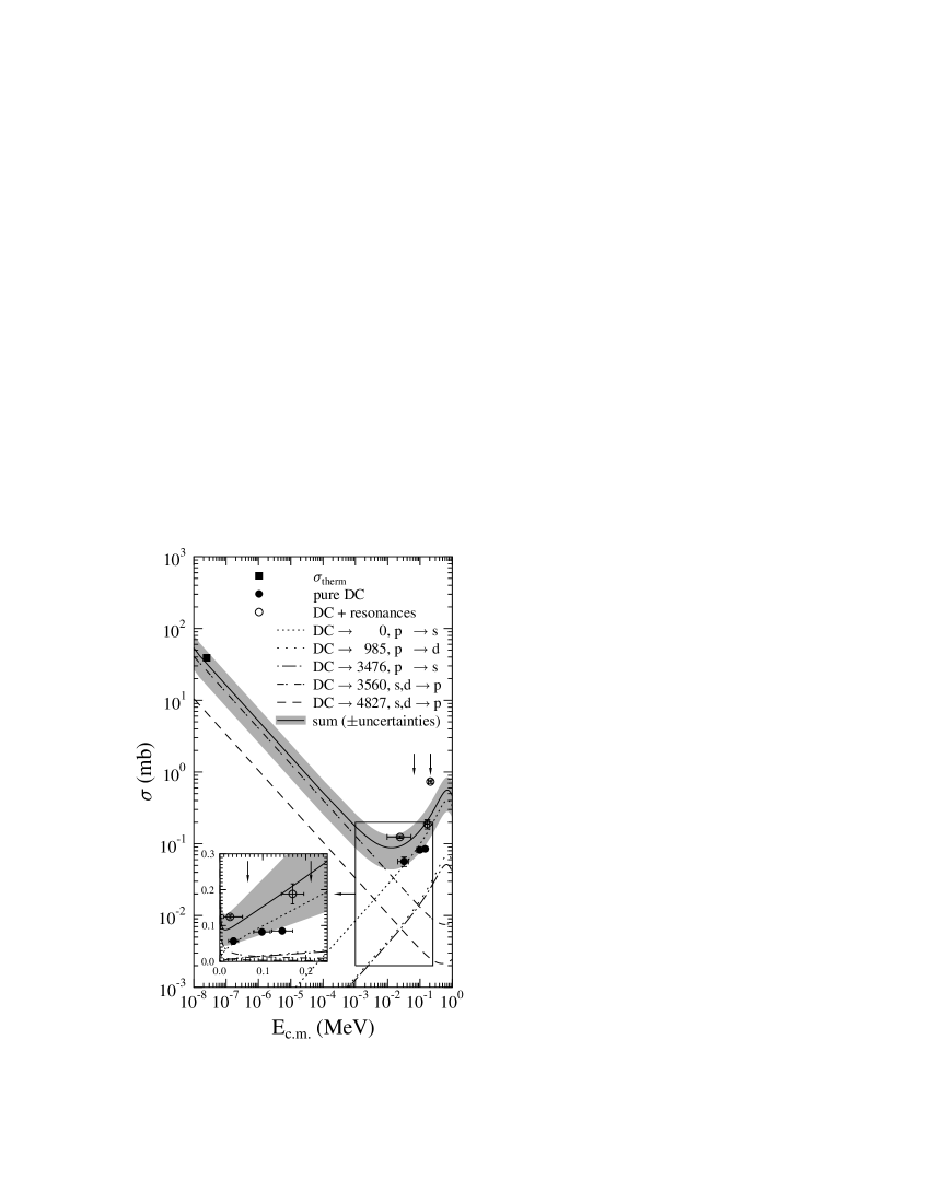
FIG. 4.: Experimental capture cross section of the reaction ²⁶Mg(n,$\gamma$)²⁷Mg compared to a DC calculation. All circles are the result of this experiment. The full circles ($\bullet$) show the non-resonant part, the open circles ($\circ$) are influenced by the known resonances at $E_{\rm{n,lab}}=68.7~{}{\rm{keV}}$ and $E_{\rm{n,lab}}=220~{}{\rm{keV}}$ [11] which are indicated by the vertical arrows. The thermal capture cross section was taken from Ref. [8]. The horizontal error bars show the FWHM of the neutron energy spectra. Note the logarithmic scale of the big figure and the linear scale of the inset; the data point at $E_{\rm{n,lab}}=208.3~{}{\rm{keV}}$ does not fit in the linear inset.

FIG. 5.: Calculated capture cross section of the ground state transition ²⁶Mg(n,$\gamma$)²⁷Mg_g.s. with $C^{2}S({\rm g.s.})=1.0$ (E1 transition from the incoming $p$-wave to the bound $s$-wave). The capture cross section depends sensitively on the potential strength parameter $\lambda$ of the incoming $p$-wave which was varied from $\lambda=0.80$ (lowest capture cross section) up to $\lambda=1.10$ in steps of 0.02 (from bottom to top, exceptions are indicated in the figure). Note that the capture cross section varies up to five orders of magnitude when the potential strength is increased/decreased by about 15% from the value for the $s$-wave ($\lambda=0.9694$)!

FIG. 6.: Scattering phase shifts $\delta_{l=1}(E)$ calculated for different potential strength parameters $\lambda$ from 0.80 to 1.10 in steps of 0.02 (from bottom to top). Note that the resonance position is shifted towards lower energies as the potential strength increases. For $\lambda=1.10$ the resonance disappears below the threshold (see also Table V).

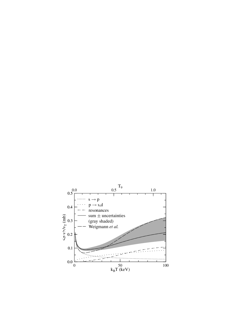
FIG. 7.: Maxwellian averaged capture cross section $<\sigma>\,=\,<\sigma\cdot v>\,/\,v_{\rm T}$, for the reaction ²⁶Mg(n,$\gamma$)²⁷Mg. The total capture cross section is given by the sum of $s$-wave capture, $p$-wave capture, and resonant contributions. For comparison we also show the result from Ref. [11].