Multifragmentation at Intermediate Energy: Dynamics or Statistics?

Nuclear Science Division
Lawrence Berkeley National Laboratory
Berkeley, California 94720

Presented at the 14^th Winter Workshop
on Nuclear Dynamics, Snowbird, Utah,
January 31- February 7, 1998

Introduction

Since the observation of a power-law behaviour in the charge distributions, characteristic of critical phenomena ${}^{\hbox{\scriptsize\cite[cite]{[\@@bibref{}{Fis67,Stu92}{}{}]}}}$, in proton induced reactions at relativistic energies, the production of multiple intermediate mass fragments (IMF) ${}^{\hbox{\scriptsize\cite[cite]{[\@@bibref{}{Bor92,Mor93}{}{}]}}}$, typically $3\leq Z\leq 20$, has been touted as a signature of the nuclear liquid-gas phase transition ${}^{\hbox{\scriptsize\cite[cite]{[\@@bibref{}{Fin82,Sie83,Pan84}{}{}]}}}$. While this may be the case in peripheral reactions e.g. projectile or spectator breakup ${}^{\hbox{\scriptsize\cite[cite]{[\@@bibref{}{Des93,Kre93,Gil94,Poc95,Ben95,Bea96c,Mas96,Bea96b,Sch96, Poc97,Hau98}{}{}]}}}$, the situation becomes less clear when one looks at more central reactions. In particular, it has been shown that the dissipative binary mechanism ${}^{\hbox{\scriptsize\cite[cite]{[\@@bibref{}{Lot92,Que93,Lec94,Pet95,Bea96}{}{}]}}}$ contributes 95% or more of the reaction cross section ${}^{\hbox{\scriptsize\cite[cite]{[\@@bibref{}{Pet95,Bea96}{}{}]}}}$. Yet, as long as the sources are thermalized, it has been shown that a characteristic signature for phase coexistence can be extracted from the charge distributions ${}^{\hbox{\scriptsize\cite[cite]{[\@@bibref{}{Pha95,Mor95b}{}{}]}}}$. The situation is further complicated by the experimental observation of a significant contribution to the fragment yields from a third source formed between the projectile and target ${}^{\hbox{\scriptsize\cite[cite]{[\@@bibref{}{Monto94,Luka97,Laro97,Tok95,Leco95,Demp96}{}{}]}}}$. Most of these observations were made using velocity plots (see for example ref. [Luka97]) which are useful in assigning a given particle to its primary source. This evidence points out the importance of dynamics in the entrance channel. Unfortunately, it tells very little about the intrinsic properties of the sources themselves. In particular, it does not disclosed the nature of the fragmentation process producing the detected “cold” IMF, i.e. at $t\rightarrow\infty$.

In the following, we will consider two contradictory claims that have been advanced recently: 1) the claim for a predominantly dynamical fragment production mechanism ${}^{\hbox{\scriptsize\cite[cite]{[\@@bibref{}{Tok96,Tok97}{}{}]}}}$; and 2) the claim for a dominant statistical and thermal process ${}^{\hbox{\scriptsize\cite[cite]{[\@@bibref{}{Mor95,Tso95,Mor97,Pha96,Bea98,Mor93b}{}{}]}}}$. We will present a new analysis in terms of Poissonian reducibility and thermal scaling, which addresses some of the criticisms of the binomial analysis ${}^{\hbox{\scriptsize\cite[cite]{[\@@bibref{}{Tok97,Tsa97,Sku97}{}{}]}}}$.

Dynamical fragment production

To make a statement about the nature and mechanism of fragmentation, it is necessary to probe directly any competition, or lack thereof, between the emission of various particle species as a function of excitation energy. The task is then to find a global observable that best follows the increase in excitation energy or dissipated energy. IMF multiplicity, $N_{IMF}$, and total transverse energy, $E_{t}$ have both been used to infer a decoupling between light charged particles (LCP) and IMF production ${}^{\hbox{\scriptsize\cite[cite]{[\@@bibref{}{Tok96,Tok97}{}{}]}}}$.

$N_{IMF}$ as global observable

Recently, it was claimed by Toke et al. ${}^{\hbox{\scriptsize\cite[cite]{[\@@bibref{}{Tok96}{}{}]}}}$ that IMF production is predominantly a dynamical process. The evidence came by looking at different particle multiplicities, and their corresponding transverse energies, as a function of IMF multiplicity.

Figure 1.: Average LCP multiplicity (upper panels), IMF multiplicity (upper left) and average transverse energy associated to LCP and IMF (bottom panels) as a function of the total transverse energy (left panels) and IMF multiplicity (right panels) for the Xe + Au reaction between 40 and 60 MeV/nucleon.

The argument was made as follows. The multiplicities of neutrons ($N_{n}$) and light charged particles ($N_{LCP}$), represent a good measurement of the thermal excitation energy of the system, $E^{*}$, as do the transverse energies of the LCPs, $E_{t}^{LCP}$. Using $N_{IMF}$ as a global variable, a fast and simultaneous saturation of $N_{n}$, $N_{LCP}$ and $E_{t}^{LCP}$ was observed in the reaction Xe+Bi at 28A MeV ${}^{\hbox{\scriptsize\cite[cite]{[\@@bibref{}{Tok96}{}{}]}}}$. This saturation occurs around $N_{IMF}$ = 2-3. The authors conclude that, since most of the IMFs (up to 12) are produced after the saturation, there is a “critical” excitation energy above which the IMFs are produced without competing with the LCPs. This apparent decoupling of IMF production from that of the LCPs is interpreted as due to the onset of a dynamical process.

We have explored the above behaviour in a systematic study of Xe+Au reactions (similar to Xe+Bi) at 40A, 50A and 60A MeV. The data were taken in two different experiments at the NSCL using the MSU Miniball 4$\pi$ array and the LBL forward array ${}^{\hbox{\scriptsize\cite[cite]{[\@@bibref{}{Sou92,Keh92}{}{}]}}}$. The right panels of Fig. 1 show the evolution of $N_{LCP}$, $E_{t}^{LCP}$ and $E_{t}^{IMF}$ as a function of $N_{IMF}$. The saturation is clearly present in both observables related to LCP. However, as the beam energy increases, the saturation point moves toward higher IMF mutiplicities. At 60A MeV, the saturation occurs at $N_{IMF}\sim$ 8. If one follows the interpretation mentioned above, one might be led to conclude that most of the IMF are produced before the saturation “critical energy” and that therefore the IMF production might be statistical and thermal in nature. In any case, the features shown in Fig. 1 are sufficiently intriguing to warrant further study.

To do so, we have performed a simulation using the SMM model ${}^{\hbox{\scriptsize\cite[cite]{[\@@bibref{}{Bon95}{}{}]}}}$. We have considered the breakup of Au nuclei with a triangular excitation energy ($E^{*}$) distribution ranging from 0.5A to 6.0A MeV (note that a flat distribution does not change the conclusion but that a triangular one is closer to the impact parameter weighted behaviour of the cross section). The maximum average number of IMFs for this simulation is about 4, similar to the Xe+Bi case. Cuts on $N_{IMF}$ were done and are shown in the right panels of Fig. 2. Here, as in the experiment, we notice a fast and simultaneous saturation of $N_{n}$, $N_{LCP}$ and $E_{t}^{LCP}$. However, the fragmentation process is, by the nature of the model, of statistical origin. Inspection of the figure reveals that saturation occurs around $N_{IMF}$=4, which corresponds to the maximum average number, $\left<N_{IMF}\right>_{max}$. In the model, the average value of $N_{IMF}$ increases with $E^{*}$ until $\left<N_{IMF}\right>_{max}$ is reached at $E^{*}_{max}$. Therefore, $N_{IMF}$ is, on average, a rough measure of excitation energy for $N_{IMF}<\left<N_{IMF}\right>_{max}$. For values of $N_{IMF}>\left<N_{IMF}\right>_{max}$, there is no increase of $E^{*}$.

For a given $E^{*}$, the IMF distribution is characterized not only by its mean but also by its variance. Although $\left<N_{IMF}\right>_{max}$=4, Fig. 2 (right panels) shows that events with up to 12 IMF are present. Cutting on $N_{IMF}$ past its average maximum value probes a nearly constant excitation energy. This is nicely illustrated by the saturation of neutron and LCP multiplicities, which are also sensitive to $E^{*}$. This is a general feature of any statistical model as pointed out by Phair et al. ${}^{\hbox{\scriptsize\cite[cite]{[\@@bibref{}{Pha98a}{}{}]}}}$. Note that the increase of $E_{t}^{IMF}$ with $N_{IMF}$ is due to the trivial autocorrelation between the two quantities.

Returning to the data (Fig. 1, right panels), as the beam energy increases, the excitation energy and IMF production increase. Therefore, in a statistical picture, the change in the “critical saturation energy” is due to the increase of excitation energy (dissipated energy) with beam energy, and correspondingly, to an increase of $\left<N_{IMF}\right>_{max}$ with excitation energy. If, for a given reaction, IMF were produced dynamically, why should the “critical saturation energy” change with beam energy?

Figure 2.: Average LCP and neutron multiplicities (upper panels), IMF multiplicity (upper left) and average transverse energy associated to LCP and IMF (bottom panels) as a function of the total transverse energy (left panels) and IMF multiplicity (right panels) for the breakup of Au nuclei in the SMM model. For details see text.

$E_{t}$ as global observable

The same authors have suggested ${}^{\hbox{\scriptsize\cite[cite]{[\@@bibref{}{Tok97}{}{}]}}}$ that the “evidence” for dynamical IMF production shown in the previous section might already be contained in the evolution of the same quantities ($N_{n}$, $N_{LCP}$, $E_{t}^{LCP}$, $N_{IMF}$ and $E_{t}^{IMF}$) as a function of the total transverse energy, $E_{t}$. Again, the authors have observed a fast and simultaneous saturation of $N_{n}$, $N_{lcp}$ and $E_{t}^{LCP}$ as a function of $E_{t}$, but a continuous increase of $E_{t}^{IMF}$ and $N_{IMF}$. In their work (ref. [Tok97], Fig. 2), they state, correctly, that if $E_{t}$ were a good measure of excitation energy, and the IMF were produced statistically, such saturations should not occur. Indeed, our statistical simulation (left panels of Fig. 2) shows that $N_{LCP}$ and $E_{t}^{LCP}$ increase monotonically with $E_{t}$ and, at no point, is $E_{t}^{IMF}$ greater than $E_{t}^{LCP}$. Thus, the behaviour of the Xe+Bi experimental results, if correct, cannot be explained by statistical models.

In fact, saturations in $N_{LCP}$ and $E_{t}^{LCP}$ are not observed in comparable data for the Xe+Au reactions as shown in Fig. 1 (left panels). $N_{LCP}$ increases smoothly with $E_{t}$, as does $E_{t}^{LCP}$. Notice that $E_{t}^{LCP}$ is always larger than $E_{t}^{IMF}$. For the Xe+Au at 50A MeV, the ratio $E_{t}^{IMF}/E_{t}^{LCP}$ is always smaller than 0.3. This result is strongly at variance with the Xe+Bi data where the IMF contribute up to 80% to the total $E_{t}$. The Xe+Bi data are also very different from preliminary results of the Xe+Au reaction at 30A MeV (sister reaction of the Xe+Bi at 28A MeV) ${}^{\hbox{\scriptsize\cite[cite]{[\@@bibref{}{Col98,Pha98b}{}{}]}}}$, whose behaviour is similar to the data at higher energies in Fig. 1.

The dramatic difference between the Xe+Bi and the Xe+Au data may be due to the experimental set-up used for the former experiment, the Dwarf Ball ${}^{\hbox{\scriptsize\cite[cite]{[\@@bibref{}{Str90}{}{}]}}}$, whose detectors are made of thin, 4mm, CsI(Tl). Such thin detectors have a punch through energy of 30A MeV for proton and alpha particles. While the thickness of these detectors is suitable for fragments, they are too small to stop LCPs in this beam energy range. If the punch through effect is not properly corrected, the total kinetic energy associated to LCPs will be severely underestimated. This, by construction, leads to a much larger percentage of the transverse energy carried by the IMFs at a given total $E_{t}$. A detailed analysis of the Xe+Au systematic, and its comparison to Xe+Bi data, including a software replica of the Dwarf Ball, in under way ${}^{\hbox{\scriptsize\cite[cite]{[\@@bibref{}{Pha98b}{}{}]}}}$. However, it is already clear that the features presented in Fig. 2 of ref. [Tok97] are due to an experimental artifact, rather than to dynamical decay.

Statistical fragment production

Another way of approaching the fragmentation process is to rely on methods that worked well at lower energies, and permitted the understanding of low energy particle evaporation and fission of a compound nucleus. At low energies, emission probabilities and excitation functions have been far more successful then kinematical variables at suggesting whether the process is statistical (compound nucleus decay) or dynamical (direct reactions) ${}^{\hbox{\scriptsize\cite[cite]{[\@@bibref{}{Mor69}{}{}]}}}$.

The increase of fission probability as a function of excitation energy (directly related to the temperature at low energies) can be cast in terms of a Boltzmann factor depending on the temperature and the fission barrier. The corresponding Arrhenius plots obtained from fission data are linear and cover a range from 2 to 6 order of magnitudes ${}^{\hbox{\scriptsize\cite[cite]{[\@@bibref{}{Mor69}{}{}]}}}$!

Recently, similar behaviour has been found in multifragmentation data ${}^{\hbox{\scriptsize\cite[cite]{[\@@bibref{}{Pha95,Mor95b,Mor95,Tso95,Mor97,Pha96,Bea98,Mor93b}{}{}]}}}$. It has been shown that the probability $P_{n}$ of emitting $n$ intermediate mass fragments (IMFs) can be reduced to the probability of emitting a single fragment through the binomial equation ${}^{\hbox{\scriptsize\cite[cite]{[\@@bibref{}{Mor95,Tso95,Mor97}{}{}]}}}$. The extracted elementary emission probabilities $p$ were also shown to give linear Arrhenius plots when $\log 1/p$ is plotted vs $1/\sqrt{E_{t}}$. In going from reducibility to thermal scaling, the only assumption needed is that $E_{t}$ is proportional to excitation energy (or temperature). We should therefore include a few words on $E_{t}$. From an experimental point of view, $E_{t}$ represents a measure of the total energy dissipated in the reaction. It can be written as follows

$$E_{t}=E_{t}^{pre-equilibrium}+E_{t}^{rotation}+E_{t}^{flow}+E_{t}^{Coulomb}+E_{t}^{thermal}$$ (1)

In other words, the thermal portion of $E_{t}$ is drowned in an ocean of other contributions, as is the thermal excitation energy itself! For example, if we take the SMM model, and try to reproduce the $\left<N_{IMF}\right>_{max}$ of a given reaction, usually the $E_{t}$ (thermal $E_{t}$) range is too small by a factor of at least 2. However, the important unanswered question is, is $E_{t}$ tracking the increase of thermal excitation energy? We believed that it does but this remains to be proven.

In the hypothesis that the temperature $T$ is proportional to $\sqrt{E_{t}}$, these linear Arrhenius plots suggest that $p$ has the Boltzmann form $p\propto\exp(-B/T)$. This form holds for many different reactions from reverse to normal kinematics and almost over the complete intermediate energy range. Similarly, the charge distributions for each fragment multiplicity $n$ and the experimental particle-particle angular correlation are also both reducible to the distribution of individual fragments and thermally scalable ${}^{\hbox{\scriptsize\cite[cite]{[\@@bibref{}{Pha95,Mor95b,Pha96}{}{}]}}}$.

However, this approach has been meet with several criticisms. First, the binomial decomposition has been performed on the $Z$-integrated fragment multiplicities (IMF), typically associated with $3\leq Z\leq 20$. Thus, the Arrhenius plot generated with the resulting one fragment probability $p$ is an average over a range of $Z$ values. A second “problem” lies in the transformation from the excitation $E^{*}$ to the transverse energy $E_{t}$. It was shown that if the width associated with this transformation is too large, than the linearity of the Arrhenius plots constructed with the elementary probability $p$ would be lost in the averaging process ${}^{\hbox{\scriptsize\cite[cite]{[\@@bibref{}{Tok97}{}{}]}}}$. While both binomial parameters $p$ and $m$ are individually susceptible to this problem, the product of the two, $\left<n\right>$ = $\left<mp\right>$ has been shown to be very resilient to the averaging process ${}^{\hbox{\scriptsize\cite[cite]{[\@@bibref{}{Tok97}{}{}]}}}$. Finally, the fact that IMFs as a category can contribute a fair amount to $E_{t}$, about 30% maximum for the Xe+Au reaction at 50A MeV, has been pointed to as a possible source of autocorrelation between $p$ and $\sqrt{E_{t}}$ leaving its interpretation questionable ${}^{\hbox{\scriptsize\cite[cite]{[\@@bibref{}{Tsa97,Sku97}{}{}]}}}$.

In the following, we will present results from a new analysis ${}^{\hbox{\scriptsize\cite[cite]{[\@@bibref{}{Bea98}{}{}]}}}$ in which we look for reducibility and thermal scaling at the level of individual fragments of charge $Z$, and, at the same time, answer in a rather elegant way the above mentioned criticisms.

Figure 3.: The ratio of the variance to the mean number of Li, C, O, Ne and Si fragments (open and solid symbols) emitted from the reaction ¹²⁹Xe+¹⁹⁷Au at 50A MeV. The star symbols show the same ratio for all IMFs ($3\leq Z\leq 20$).

Poissonian reducibility

We analyze the fragment multiplicity distributions for each individual fragment $Z$ value. This restriction has the rather dramatic effect of decreasing the elementary probability $p$, compared to that associated with the total IMF value, to the point where the variance over the mean for any $Z$ is very close to one for all values of $E_{t}$ ${}^{\hbox{\scriptsize\cite[cite]{[\@@bibref{}{Mor97,Bea98}{}{}]}}}$(Fig. 3). This means that the binomial distribution tends to its Poissonian limit. In this limit, the quantities $m$ and $p$ are not individually extracted, but it is rather the quantity $\left<n\right>$ = $\left<mp\right>$ that is obtained. The Poisson distribution is expressed as

$$P_{n}(Z)=\frac{\left<n_{Z}\right>^{n}e^{-\left<n_{Z}\right>}}{n!}$$ (2)

where $n$ is the number of fragments of a given $Z$ and the average value $\left<n_{Z}\right>$ is a function of $E_{t}$. We can verify the ability of Eq. 1 to reproduce the n-fold probability distribution, $P_{n}$, for Li fragments in Fig. 4 (left panel). The symbols are experimental n-fold probabilities, while the lines are the probabilities obtained by introducing the experimental average values in Eq. 1. For all the reactions studied, Poissonian fits (Eq. 1) were excellent for all $Z$ values starting from $Z$=3 up to $Z$=14 over the entire range of $E_{t}$ ${}^{\hbox{\scriptsize\cite[cite]{[\@@bibref{}{Bea98}{}{}]}}}$. $\left<n_{Z}\right>$ is now the only quantity needed to describe the emission probabilities $P_{n}$ of charge $Z$. Thus we conclude that reducibility (now Poissonian reducibility) is verified at the level of individual $Z$ values for many different systems. Moreover, reducibility is tested for each ($Z$,$E_{t}$) combination. For example, in Fig. 4, the reducibility is tested 40 times just for $Z$=3. Reducibility, binomial or Poissonian, is an experimental observation, demonstrating that fragment emission is a stochastic process.

Figure 4.: Left panel: The excitation functions $P_{n}$ for lithium emission from the reaction ¹²⁹Xe+¹⁹⁷Au at 50 A MeV. The lines are Poisson fits to data. The ratio of one n-fold to the next is shown in the upper right panel and the appropriate scaling in the lower right panel. The line in the lower right panel is the experimental average number, $\left<n_{Z}\right>$.

Thermal scaling

In order to verify thermal scaling, we can first look at the ratio of one fold to the next, $P_{n+1}/P_{n}$ as in ref. [Mor93b]. The results yield linear plots versus $1/\sqrt{E_{t}}$ as shown in Fig. 4 (right panel). However, these plots are not all independent; in fact, from Eq. 1, one find that $P_{n+1}/P_{n}=\left<n\right>/n+1$. Correcting the ratio by the trivial $n+1$ factor collapses all the curves into a single one, which follows nicely the line of the experimental average values. Consequently, we generate Arrhenius plots by plotting directly $\log\left<n\right>$ vs $1/\sqrt{E_{t}}$. The left panel of Fig. 5 gives a family of these plots for the Xe+Au reaction at 50A MeV, and $Z$ values extending from $Z$=3 to $Z$=14. These Arrhenius plots are strikingly linear over factors of 10 to 60, and their slopes increase smoothly with increasing $Z$ value. The overall linear trend demonstrates that thermal scaling is also present when individual fragments of a specific $Z$ are considered.

The advantage of this procedure is readily apparent. For any given reaction, thermal scaling is verifiable for as many atomic numbers as are experimentally accessible (12 in this case). Futhermore, to generate this figure, Poissonian reducibility has been tested 480 times. This is an extraordinary level of verification of the empirical reducibility and thermal scaling with the variable $E_{t}$.

Additionally, as discussed above, $\left<n_{Z}\right>$ is free of any distortion due to averaging when going from $E^{*}$ to $E_{t}$ ${}^{\hbox{\scriptsize\cite[cite]{[\@@bibref{}{Tok97}{}{}]}}}$. Also, because of the dominance of the zero fold probability, the average contribution of a particular $Z$ to $E_{t}$ is very small, $\leq$ 5%, thus minimising the risk of autocorrelation. Still, to be sure that there is no autocorrelation, we have repeated the analysis for Xe+Au at 50A MeV by: i) removing from $E_{t}$ all contributions from the specific $Z$ ($E_{t}^{Z}$) that we have selected (Fig. 5, middle panel). ii) by using only the $E_{t}$ of the light charge particles, $E_{t}^{LCP}$ (Fig. 5, right panel). In both cases, the Arrhenius plots remain linear for almost the entire range of $E_{t}$, and $\left<n_{Z}\right>$ changes by factors of 10 to 50. These results are similar to those obtained using the total $E_{t}$. We conclude that the linearity of the Arrhenius plots is not due to autocorrelation but to a thermal/statistical emission process dominated by phase space.

Figure 5.: The average yield per event of different elements (symbols) as a function of $1/\sqrt{E_{t}}$ for the reaction Xe+Au data at 50A MeV using the total transverse energy $E_{t}$ (left), the transverse energy of all charged particles excluding the Z that we have selected $E_{t}^{Z}$ (middle) and (right) that only of the light charged particles (LCPs) $E_{t}^{LCP}$. The lines are fits to the data using a Boltzmann form for $\left<n_{Z}\right>$.

We have observed experimentally that the maximum values of the new $E_{t}$ scales (either $E_{t}^{Z}$ or $E_{t}^{LCP}$) correspond to events in which fragments of a given $Z$ (or all IMFs) are absent. Therefore, in our attempt to avoid autocorrelation by excluding from $E_{t}$ all IMFs ($E_{t}^{LCP}$) or the $Z$ value under investigation ($E_{t}^{Z}$), we have introduced another kind of autocorrelation. For example, excluding from $E_{t}$ all fragments of charge $Z$ to produce $E_{t}^{Z}$ necessarily requires that for those events where $E_{t}^{Z}\approx E_{t}$, the yield $n_{Z}\rightarrow 0$. This produces the visible turnover of the Arrhenius plots in the bottom panels of Fig. 5 (the same argument also applies to $E_{t}^{LCP}$).

Finally, even though we have constructed the Arrhenius plots from three different $E_{t}$ scales, the slopes associated with these plots always become steeper with increasing $Z$ values. This is what we would expect if the slopes parameters are related to physical fragmentation barriers. Moreover, the rate of change of the slopes with various $E_{t}$ scale is the same. This is shown in Fig. 6 where the various sets of barriers have been normalized to $Z$=6 from the full $E_{t}$ scale.

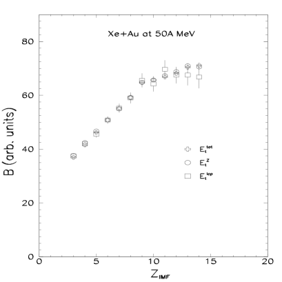
Figure 6.: Slopes of the Arrhenius plots, normalized to $Z$=6, for Xe+Au at 50A MeV as a function of $Z$ using the indicated definitions of $E_{t}$.

Summary and Outlook

In heavy ion reactions at intermediate energies, a complex dynamical behaviour is observed in the entrance channel. However, in order to understand the nature of the fragmentation process, one must rely on observables other than velocity plots, and their associated kinematic variables.

The evolution of multiplicities of neutrons, light charged particles or IMF and of their corresponding transverse energies with $N_{IMF}$ or $E_{t}$ does not provide convincing evidence for the claim of a dynamical IMF production. In the first case ${}^{\hbox{\scriptsize\cite[cite]{[\@@bibref{}{Tok96}{}{}]}}}$, the behaviour is a rather general one and is found in any statistical model. In the second case ${}^{\hbox{\scriptsize\cite[cite]{[\@@bibref{}{Tok97}{}{}]}}}$, the anomalous features associated with dynamical IMF production are most likely due to an experimental artifact.

Armed with observables that have have been successful for low energy nuclear reactions, we have used the probabilities and excitation functions to probe the nature of the fragmentation process. The n-fold probabilities of individual $Z$ values are shown to follow Poissonian distributions, and as such, are reducible. The experimental observation of Poissonian reducibility means that IMF production is dominated by a stochastic process. Of course stochasticity falls directly in the realm of statistical decay. It is less clear how it would fare within the framework of a dynamical model without appealing for chaoticity or ergodicity. Futhermore, the thermal scaling of $\left<n_{Z}\right>$ suggest that it has the Boltzmann form

$$\left<n_{Z}\right>\propto e^{-B_{Z}/T}$$ (3)

It is important to recall that by considering individual $Z$ values, one obtains Arrhenius plots free of distortion or autocorrelation. Additionnally, this form permits the extraction of a fragmentation “barrier” $B_{Z}$ for each $Z$. The behaviour described in Eq. 2 is similar to that observed in the fission process of ref. [Mor69]. The emission probability of a given $Z$ is controlled by its emission barrier and the temperature.

Acknowledgments

This work was supported by the Director, Office of Energy Research, Office of High Energy and Nuclear Physics, Nuclear Physics Division of the US Department of Energy, under contract DE-AC03-76SF00098. One of us (L.B) acknowledge a fellowship from the National Sciences and Engineering Research Council (NSERC), Canada.

REFERENCES

1. M.E. Fisher,  Physica 3, 225 (1967).

2. D. Stuffer and A. Aharony,  Introduction to percolation theory, 2nd Ed. (Taylor and Francis, London, 1992) pp.181.

3. J.E. Finn et al.,  Phys. Rev. Lett 49, 1321 (1982).

4. J.P. Siemens,  Nature 305, 410 (1983).

5. A.D. Panagiotou et al.,  Phys. Rev. Lett 52, 496 (1984).

6. B. Borderie, Ann, de Phys. 17, 349 (1992).

7. L.G. Moretto and G.J. Wozniak, Ann. Rev. Nucl. Part. Sci. 43, 379 (1993).

8. P. Désesquelles et al.,  Phys. Rev. C 48, 1828 (1993).

9. P. Kreutz et al.,  Nucl. Phys. A556, 672 (1993).

10. M.L. Gilkes et al.,  Phys. Rev. Lett 73, 1590 (1994).

11. J. Pochodzalla et al.,  Phys. Rev. Lett 75, 1040 (1995).

12. J. Benlliure,  Ph.D. thesis, University of Valencia, Spain, 1995 (unpublished).

13. L. Beaulieu,  Ph.D. thesis, Universit’e Laval, Canada, 1996 (unpublished).

14. P.F. Mastinu et al,  Phys. Rev. Lett. 76, 2646 (1996).

15. L. Beaulieu et al.,  Phys. Rev. C 54, R973 (1996).

16. A. Schüttauf et al.,  Nucl. Phys. A 607, 457 (1996).

17. J. Pochodzalla,  Prog. Part. Nucl. Phys. 39, 443 (1997).

18. J.A. Hauger et al.,  Phys. Rev. C 57, 764 (1998).

19. B. Lott et al.,  Phys. Rev. Lett. 68, 3141 (1992).

20. B.M. Quednau et al.,  Phys. Lett. B309, 10 (1993).

21. J.F. Lecolley et al.,  Phys. Lett. B325, 317 (1994).

22. J. Péter et al.,  Nucl. Phys. A593, 95 (1995).

23. L. Beaulieu et al.,  Phys. Rev. Lett. 77, 462 (1996).

24. L. Phair et al., Phys. Rev. Lett. 75, 213 (1995).

25. L.G. Moretto et al., Phys. Rev. Lett. 76, 372 (1996).

26. C.P. Montoya et al., Phys. Rev. Lett 73, 3070 (1994).

27. J. Lukasik et al., Phys. Rev. C 55, 1906 (1997).

28. Y. Larochelle et al., Phys. Rev. C 55, 1869 (1997).

29. J. Toke et al., Phys. Rev. Lett. 75, 2920 (1995).

30. J.F. Lecolley et al., Phys. Lett. B 354, 202 (1995).

31. J.F. Dempsey et al., Phys. Rev. C 54, 1710 (1996).

32. J. Toke et al., Phys. Rev. Lett 77, 3514 (1996).

33. J. Toke et al., Phys. Rev. C 56, R1683 (1997).

34. L.G. Moretto et al., Phys. Rev. Lett. 74, 1530 (1995).

35. K. Tso et al., Phys. Lett. B 361, 25 (1995).

36. L.G. Moretto, et al., Phys. Rep. 287, 249 (1997).

37. L. Phair et al., Phys. Rev. Lett 77, 822 (1996).

38. L. Beaulieu et al., Submitted to Phys. Rev. Lett.

39. L.G. Moretto, et al., Phys. Rev. Lett. 71, 3935 (1993).

40. M.B. Tsang et al., Phys. Rev. Lett. 80, 1178 (1998)

41. W. Skulski et al., to appear in Proc. 13th Workshop on Nuclear Dynamics, Key West, Florida (1997).

42. R.T. de Souza et al., Nucl. Inst. Meth. A 311, 109 (1992).

43. W.C. Kehoe et al., Nucl. Inst. Meth. A 311, 258 (1992).

44. J.P. Bondorf et al., Phys. Rep. 257, 133 (1995).

45. L. Phair et al., Accepted in Phys. Rev. Lett..

46. N. Colonna, private communication.

47. L. Phair et al., to be published.

48. D.W. Stracener et al., Nucl. Inst. Meth. A 294, 485 (1990).

49. L.G. Moretto, Phys. Rev. 179, 1176 (1969).