Proton and Antiproton Distributions at Mid-Rapidity in Proton-Nucleus and Sulphur-Nucleus Collisions

Abstract

Experiment NA44 has measured proton and antiproton distributions at mid-rapidity in sulphur and proton collisions with nuclear targets at 200 and 450 GeV/c per nucleon respectively. The inverse slopes of transverse mass distributions increase with system size for both protons and antiprotons but are slightly lower for antiprotons. This could happen if antiprotons are annihilated in the nuclear medium. The antiproton yield increases with system size and centrality and is largest at mid-rapidity. The proton yield also increases with system size and centrality, but decreases from backward rapidity to mid-rapidity. The stopping of protons at these energies lies between the full stopping and nuclear transparency scenarios. The data are in reasonable agreement with RQMD predictions except for the antiproton yields from sulphur-nucleus collisions.

I Introduction

Nucleus-nucleus collisions at ultrarelativistic energies create hadronic matter at high energy density. The distributions of baryons at mid-rapidity provide a sensitive probe of the collision dynamics. In particular, the stopping power determines how much of the incoming longitudinal energy is available for excitation of the system. These collisions have been described by microscopic models incorporating hadron production and rescattering, see for example [1]. The data reported here impose constraints on the amount of stopping of baryons in such models.

Enhanced production of antibaryons may indicate formation of a state of matter in which the quarks and gluons are deconfined [2, 3, 4, 5]. Such enhancement may be hidden, however, by antibaryon annihilation with baryons [6, 7]; the antiproton survival probability is sensitive to both the collision environment and the antiproton formation time. The antiproton and proton distributions may also reflect the degree of thermalization achieved and, by comparing distributions from light and heavy systems, allow detailed studies of rescattering.

We present proton and antiproton measurements using the NA44 spectrometer from $pBe$ (to approximate $pp$), proton-nucleus and nucleus-nucleus interactions. This allows a systematic study as a function of the size of the central region and different conditions in the surrounding hadronic matter.

These systematic studies are aided by use of an event generator. The RQMD model, version 1.08 [1], is a microscopic phase space approach, based on resonance and string excitation and fragmentation with subsequent hadronic collisions. RQMD includes annihilation of antiprotons in the hadronic medium when they collide with baryons [7]. We study a feature of RQMD called color ropes by the authors of the model. RQMD uses a string model of particle production from each nucleon-nucleon collision. In a heavy-ion collision, where there are numerous nucleon-nucleon collisions, the density of these strings is high and multiple strings overlap. Overlapping strings do not fragment independently but form ‘ropes’, chromoelectric flux-tubes whose sources are color octet charge states rather than the color singlet charges of normal strings [8]. These ropes represent a collective effect in nucleus-nucleus collisions, and have been shown to enhance both strangeness and baryon pair production [8].

II Experiment

The NA44 experiment is shown in Figure 1. Three conventional dipole magnets (D1, D2, and D3) and three superconducting quadrupoles (Q1, Q2, and Q3) analyze the momentum and create a magnified image of the target in the spectrometer. The magnets focus particles from the target onto the first hodoscope (H1) such that the horizontal position along the hodoscope gives the total momentum. Two other hodoscopes (H2, H3) measure the angle of the track. The momentum acceptance is $\pm$ 20% of the nominal momentum setting. The angular coverage is approximately -5 to +78 mrad with respect to the beam in the horizontal plane and $\pm$ 5 mrad vertically. Only particles of a fixed charge sign are detected in a given spectrometer setting. Four settings are used to cover the mid-rapidity region in the $p_{T}$ range 0 to 1.6 GeV. Figure 2 shows the acceptance of the spectrometer in the $y-p_{T}$ plane for the 4 and 8 GeV/c momentum settings when the spectrometer axis is at 44 and 131 mrad with respect to the beam.

For the sulphur-nucleus data, the beam rate and time-of-flight start are determined using a Cherenkov beam counter (CX), with time resolution of approximately 35 ps [9]. For the proton-nucleus data, a scintillator counter is used to measure the beam rate. A second scintillator (T₀) is used to trigger on central events in sulphur-nucleus collisions by requiring a large pulse height (high charged particle multiplicity). The pseudorapidity coverage of T₀ is roughly 1.3 to 3.5. For proton beams, T₀ provides the interaction trigger by requiring that at least one charged particle hit the scintillator, and also provides the time-of-flight start with a time resolution of approximately 100 ps. A silicon pad detector measures the charged-particle multiplicity with $2\pi$ azimuthal acceptance in the pseudorapidity range $1.8<\eta<3.3$.

The three scintillator hodoscopes (H1, H2 and H3) are used to track the particles and are divided into 50, 60 and 50 slats, respectively. The hodoscopes also provide time-of-flight with a time resolution of approximately 100 ps; particle identification relies primarily upon the third hodoscope. Two Cherenkov counters differentiate kaons and protons (C1: freon-12 at 1.4 or 2.7 atm, depending on the spectrometer setting), and reject electrons and pions (C2: nitrogen/neon mixture at 1.0 or 1.3 atm). An appropriate combination of C1 and C2 is used for each spectrometer setting to trigger on events with no pions or electrons in the spectrometer. Particles are identified by their time-of-flight, in combination with the Cherenkov information. Figure 3 illustrates the particle identification after pions have been vetoed by the Cherenkovs; kaons and protons are clearly separated. More details about the spectrometer are available in [10].

III Data Analysis

The proton and antiproton data samples after particle identification and quality cuts are shown in Table I. Also shown for each data set is the target thickness and the centrality, expressed as a fraction of the total inelastic cross-section.

Tracks are reconstructed from the hit positions on the three hodoscopes, constrained by straight-line trajectories after the magnets. In order to construct the invariant cross-section, the raw distributions are corrected using a Monte Carlo simulation of the detector response. Simulated tracks are passed through the full analysis software chain and used to correct the data for geometrical acceptance, reconstruction efficiency and momentum resolution. Particles are generated according to an exponential distribution in transverse mass, $m_{T}=\sqrt{p_{T}^{2}+m_{p}^{2}}$, with the coefficient of the exponent determined iteratively from the data.

The Cherenkovs reject pions with an efficiency of greater than 98% at the trigger level. Further offline selection reduces the pions to a few percent of the kaons. After time-of-flight and Cherenkov cuts, the residual kaon contamination of the proton sample is less than 3%.

The invariant cross-sections are presented as a function of $m_{T}$ - $m_{p}$, where $m_{p}$ is the mass of the proton. The absolute normalization of each spectrum is calculated using the number of beam particles, the target thickness, the fraction of interactions satisfying the trigger, and the measured live-time of the data-acquisition system. For the $SA$ data, the centrality selection is determined by comparing the pulse height distribution in the T₀ counter for central and unbiased beam triggers. For $pA$ systems, the fraction of inelastic collisions producing at least one hit in the interaction (T₀) counter is modeled with the event generators RQMD [1] and FRITIOF [11, 12]. The errors on the centralities for the $pA$ data in Table I reflect the systematic uncertainty on this fraction from comparing the two models. The $pA$ data are also corrected for the efficiency of the T₀ counter. The resulting centrality fractions are indicated in Table I.

The proton-nucleus data are corrected for non-target background. The largest corrections are 7.4% and 6.7% on the absolute cross-sections for protons and antiprotons from $pBe$ collisions. This correction does not affect the shape of the distribution. The corrections to the nucleus-nucleus data are negligible. The cross-sections are also corrected for the proton identification efficiency, and for the effects of selecting events with no accompanying pion or electron. The pion (electron) veto correction is determined from the number of protons in runs for which the pions (electrons) are not vetoed. The effect of hadronic interactions of the produced particles in the material of the spectrometer has been studied using a detailed GEANT simulation. These interactions, including annihilation of antiprotons in the spectrometer material, do not distort the shape of the measured transverse mass distributions but result in a reduction in the observed yields of about 11% for protons and 17% for antiprotons. The data are corrected for these losses.

The invariant cross-sections, measured in the NA44 acceptance, are generally well described by exponentials in transverse mass (see Equation 1). The proton and antiproton rapidity densities (dN/dy) are calculated by integration of the normalized $m_{T}$ distributions, with the fitted coefficient of the exponent (the ‘inverse slope’) used to extrapolate to high $m_{T}$, beyond the region of measurement. The statistical error on this extrapolation is calculated using the full error matrix from the fit of Equation 1 (see Section VI) to the $m_{T}$ spectrum. The corresponding systematic error is included in Table II.

IV Systematic Errors

The momentum scale of the spectrometer is verified with a second, independent measurement of the momentum using the multiwire proportional chambers (MWPCs 1-4 in Figure 1) and dipole magnet (D3), yielding a systematic error of 1.6% on the $p_{T}$ scale. Since the NA44 spectrometer has acceptance for both positive and negative $p_{X}$, a systematic offset in $p_{T}$ can be checked by requiring symmetry around $p_{X}=0$. The resulting uncertainty on the origin of the $p_{T}$ scale is 7 MeV/c for the 8 GeV setting. A detailed Monte Carlo simulation, including multiple scattering and detector granularity, is used to correct for the finite resolution of the spectrometer, and introduces a systematic error in $p_{T}$ of 0.15%.

Systematic errors on the inverse slopes of the transverse mass distributions are estimated by comparing the inverse slope determined from the 131 mrad data to the inverse slope determined from both angle settings, and are less than 5%(15%) for the 8 GeV(4 GeV) setting data. The systematic errors due to the spectrometer acceptance correction are estimated from the sensitivity of the extracted slope to the fit range used, and by measuring the slope determined from the ratio of the cross-sections corresponding to the ‘central ray’ of the spectrometer at both the 131 and 44 mrad settings. In this ratio the acceptance corrections cancel since the particles have the same path through the spectrometer. The total uncertainty is 10 MeV/c for the mid-rapidity ($y$=2.3-2.9) data, and 10-20 MeV/c for the lower rapidity ($y$=1.9-2.3) data.

The error in the absolute normalizations is dominated by the uncertainty in the fraction of the total cross-section selected by the NA44 centrality trigger, and by the pion and electron veto corrections. The relative error in the centrality is 6% for both the $SS$ and $SPb$ data, resulting in a systematic uncertainty of 6% in dN/dy. For the proton-nucleus data, the trigger bias is determined by modeling the acceptance of the T₀ counter, as described above. The resulting dN/dy values are sensitive to the charged particle distribution from the two models, giving an uncertainty of 1.5% for the $pBe$ data, increasing to 3% for $pPb$. Corrections for the fraction of events vetoed by pions are significant only for the sulphur-nucleus data at the 44 mrad setting. The uncertainties in these corrections are 10% for $SPb$ collisions and 5% for $SS$ collisions. Additional errors on the dN/dy values arise from a 5% uncertainty in the determination of the data-acquisition live-time, and a 5% beam rate dependence of the pion veto correction for the $SPb$ data. For the $pA$ data, there is an additional 6% error due to the correction for the efficiency of the interaction counter. The correction for non-target background contributes a negligible systematic error to the absolute cross-sections for proton-nucleus data. The total systematic errors on the measured inverse slopes and dN/dy values are given in Table II.

V Feed-Down from Weak Decays

Weak decays of strange baryons are a significant source of protons and antiprotons, and contribute to the yields measured in the NA44 spectrometer. A strange baryon may travel several centimeters from the target before decaying weakly to a proton and a pion. Such a proton may be reconstructed in the spectrometer with the wrong momentum. The sensitivity of the data to this feed-down has been studied using a GEANT simulation of the spectrometer with particle distributions and yields taken from RQMD. Of the strange baryons, only $\Lambda^{0}$ and $\Sigma^{+}$ decay weakly to protons (with the corresponding antiparticles decaying to antiprotons). Heavier strange baryons also contribute via sequential decays.

The fraction of the measured protons (antiprotons) arising from these decays is calculated as a function of rapidity and transverse momentum within the NA44 acceptance, and used to determine ‘feed-down factors’ for the $m_{T}$ and dN/dy distributions. These are multiplicative factors which provide an estimate of the contribution of $\Lambda$ and $\Sigma$ decays to the measured distributions, and could be applied to the numbers in Tables IV and V to estimate the inverse slopes and yields of ‘direct’ protons (antiprotons). Figure 4 shows the effect of feed-down from weak decays on the RQMD proton and antiproton transverse mass distributions for $SPb$ collisions. Including $\Lambda$ and $\Sigma$ decays tends to make the distributions steeper since the protons arising from weak decays contribute more at low $p_{T}$. Table III shows the feed-down factors for the inverse slopes and yields of the data due to $\Lambda$ and $\Sigma$ decays. The values are calculated using the $\Lambda/p$ and $\Sigma/p$ ratios from RQMD. The ‘errors’ reflect the result of increasing and decreasing the $(\Lambda+\Sigma)/p$ ratio in the model by a factor of 1.5. This factor of 1.5 is consistent with the scale of the discrepancies in the published data on $\Lambda$ production in nucleus-nucleus collisions. For central $SS$ collisions, RQMD is consistent with the $\Lambda/p$ ratio measured by NA35 [13]. However for $SPb$, there is a factor of 2 discrepancy between the measurement of $\Lambda$ production by NA36 [14] and the scaled $SAg$ data of NA35. The RQMD prediction lies between the results of the two experiments. The feed-down factors have been calculated explicitly for protons from $pBe,pPb$ and $SPb$ using the complete GEANT simulation, and are scaled according to the respective RQMD ($\Lambda+\Sigma)/p$ ratios for protons from $pS$ and $SS$, and for antiprotons from all systems. A factor of 1.5 variation in the ($\bar{\Lambda}+\bar{\Sigma})/\bar{p}$ ratio is also assumed in calculating the antiproton factors. The $m_{T}$ dependence of the feed-down factors is mainly determined by the experimental acceptance and not by the $m_{T}$ dependence of the ($\Lambda+\Sigma)/p$ ratio from RQMD.

As these factors necessarily contain some dependence on models they have not been applied to the data but are listed in Table III so that the reader can appreciate the sensitivity of the data to $\Lambda$ and $\Sigma$ decays.

VI Results

The invariant cross-sections for protons and antiprotons from $pBe$, $pS$, $pPb$, $SS$ and $SPb$ collisions are shown in Figures 5 and 6 as a function of $m_{T}$ - $m_{p}$. The transverse mass distributions are generally well described by exponentials in the region of the NA44 acceptance:

$$\frac{1}{\sigma}\frac{Ed^{3}\sigma}{dp^{3}}=Ce^{-(m_{T}-m_{p})/T}$$ (1)

where C is a constant and $T$ the inverse logarithmic slope. The inverse slope parameters obtained by fitting the proton and antiproton data to Equation 1 are given in Table IV, and plotted in Figure 7. The inverse slopes for both protons and antiprotons increase with system size. For protons, the inverse slopes are higher at mid-rapidity ($y$=2.3-2.9) than at more backward rapidities ($y$=1.9-2.3). This effect is not seen for antiprotons, where the inverse slopes are similar in the two rapidity intervals. Note that the errors on the backward rapidity data are significant. The inverse slopes for antiprotons are generally somewhat lower than for protons at mid-rapidity, but are comparable in the backward rapidity interval.

The proton and antiproton rapidity densities (dN/dy) are listed in Table V and plotted in Figure 8. Proton yields increase with system size, and are significantly larger in nucleus-nucleus collisions than in proton-nucleus collisions. More protons are produced in the backward rapidity interval ($y$=1.9-2.3) than at mid-rapidity ($y$=2.3-2.9), particularly for proton-nucleus collisions. The antiproton yields are lower than the proton yields and grow less rapidly with increasing system size: the increase in the antiproton yield between $pBe$ and $pPb$ is less than 50%. Comparing antiproton yields in the two rapidity intervals, there is essentially no difference for proton-nucleus collisions. In nucleus-nucleus collisions however, antiproton production is notably smaller backwards of mid-rapidity.

Figure 9 shows the ratio of $\bar{p}$ to $p$ yields for the various projectile-target systems. Note that the systematic errors described in Table II cancel in this ratio. The $\bar{p}/p$ ratio decreases by a factor of 4 from $pBe$ to $SPb$. Most of this decrease with system size occurs between $pPb$ and $SS$. The target dependence of the ratio is stronger in sulphur-nucleus than in proton-nucleus collisions. Comparing the two rapidity intervals, the $\bar{p}/p$ ratio is larger at mid-rapidity in all cases.

The beam momentum for the $pA$ data is 450 GeV/c, corresponding to a beam rapidity of 7, while for the $SA$ data the beam momentum is 200 GeV/c per nucleon, corresponding to a beam rapidity of 6. The energy dependence of proton and antiproton production in $pp$ collisions has been studied at the ISR [15]. Using the parametrizations of the proton and antiproton cross-sections as a function of center-of-mass energy from [15], the effect of the different beam momenta for the $pA$ and $AA$ data on the systematic behaviour of the $\bar{p}/p$ ratio can be estimated. Decreasing the beam momentum from 450 to 200 GeV/c per nucleon, this energy scaling implies that the $\bar{p}$ yield decreases by $12\pm 1\%$ and the $p$ yield decreases by $1.5\pm 0.1\%$. Thus the decrease in beam energy cannot explain the decrease of the $\bar{p}/p$ ratio. Rather it reflects the fact that at mid-rapidity most protons are not produced but originate from the target or projectile.

In order to study the centrality dependence of proton and antiproton production, the $SPb$ data are divided into two subsamples containing the 11-6% and 6-0% most central collisions respectively. The inverse slopes show no centrality dependence between the two subsamples. Figure 10 shows the proton and antiproton yields for these two different centrality selections. Production of both protons and antiprotons increases with centrality, although the yield of protons rises faster.

VII Discussion

The precision of the data and the range of the systems studied provide strong constraints on models of proton and antiproton production, rescattering and annihilation. We have compared our data in detail to the RQMD model. Figure 11 compares the transverse mass distributions of protons and antiprotons from $SPb$ collisions to predictions from RQMD with and without rope formation. The contribution of feed-down from $\Lambda$ and $\Sigma$ decays is included in the model predictions, determined using the GEANT simulation described above. The shapes of the spectra are generally reproduced by the model. This is true also for the lighter collision systems. The RQMD distributions are then used to determine inverse slopes and yields from the model in the same way as for the data.

Comparing different collision systems, the inverse slopes of both protons and antiprotons increase with system size. The relative increase, from $pBe$ to $SPb$, is similar in both cases. NA44 has previously reported an increase in the inverse slopes of kaons, protons and antiprotons produced at mid-rapidity in symmetric collision systems [18]. These data extend this trend to asymmetric systems, and to more backward rapidities ($y$=1.9-2.3). For symmetric systems, the inverse slopes of protons and antiprotons are equal, while for the asymmetric systems $pS,pPb$ and $SPb$ at $y$=2.3-2.9 the inverse slopes of protons are higher than those of antiprotons.

The increase of the proton inverse slope with system size, which continues through $PbPb$ collisions [18], is a result of the increasing number of produced particles and consequent rescattering. The large number of secondary collisions causes the hadronic system to expand [10, 18, 19], and the velocity boost from this collective expansion is visible as an increased inverse slope in the proton $m_{T}$ distributions. One would expect this effect to be concentrated at mid-rapidity, and this is supported by the data which show that the inverse slopes of protons are higher at $y$=2.3-2.9 than at $y$=1.9-2.3. Though the antiproton inverse slope is also increased by secondary collisions, the RQMD model predicts that the observed antiprotons have suffered fewer rescatterings than the observed protons. This is because secondary collisions with baryons can annihilate the antiprotons, and the number of baryons at mid-rapidity in the nucleus-nucleus collisions is substantial [18]. This may explain why the inverse slopes of antiprotons do not increase from $y$=1.9-2.3 to $y$=2.3-2.9.

RQMD reproduces the trend of increasing inverse slope with system size (Table IV and Figure 7), and is in reasonable agreement on the absolute values of the inverse slopes, with the exception of the backward rapidity ($y$=1.9-2.3) protons from sulphur-nucleus collisions, where the model predicts larger inverse slopes than are measured experimentally. For $SS$ and $SPb$ at $y$=1.9-2.3, the RQMD proton distributions tend to deviate from exponentials in transverse mass, showing larger inverse slopes at low $m_{T}$ (within the NA44 acceptance) than at high $m_{T}$. For RQMD, there is no significant difference in the inverse slopes if rope formation is turned off. This might seem surprising for antiprotons since if rope formation is included, almost all antiprotons originate from ropes, and the production mechanisms of antiprotons from ropes and from conventional sources are very different. However, rescattering would tend to mask any difference in the initial $m_{T}$ distribution of antiprotons produced from either ropes or conventional sources.

The yields of protons and antiprotons both increase with system size, the proton yield rising faster. The increase of both yields and inverse slopes with target size is much stronger in $SA$ than in $pA$ collisions since target nucleons may be struck by more than one projectile nucleon. The $\bar{p}/p$ ratio decreases with system size, and is lower towards target rapidity than at mid-rapidity. This implies that most of the protons at mid-rapidity are not produced in the collision, but are remnants of the initial nuclei. The fraction and absolute numbers of such ‘original’ protons decreases from $y$=1.9-2.3 to $y$=2.3-2.9, indicating that the stopping of protons at these energies is incomplete. For $pA$ collisions, the antiproton yield is essentially constant from $y$=1.9-2.3 to $y$=2.3-2.9, whereas for $SA$ collisions more antiprotons are produced at $y$=2.3-2.9.

For the $SA$ data, no change in the inverse slopes of protons and antiprotons with centrality is seen within the 11% most central $SPb$, and 8% most central $SS$, collisions. Both proton and antiproton yields increase with centrality. The increase is larger for protons than for antiprotons, and both particles show a larger increase at $y$=2.3-2.9 than at $y$=1.9-2.3.

RQMD predictions for proton and antiproton yields, with and without color ropes, are shown in Table VI and Figure 8. The proton yields are generally well described by the model in both $pA$ and $SA$ collisions, although there is a tendency for RQMD to overpredict the yield in the more backward rapidity interval for sulphur-nucleus collisions. Antiproton yields from $pA$ collisions are also in reasonable agreement with RQMD, however the data show a somewhat weaker target dependence than the model. The antiproton yield in $SS$ collisions is consistent with the RQMD prediction without ropes, whereas the $SPb$ yield is between the rope and no-rope predictions. With no rope formation, it is possible that RQMD could reproduce the observed $SA$ antiproton yields with a smaller annihilation cross-section in the model. If, however, the rope hypothesis is valid, then either RQMD overpredicts antiproton production in nucleus-nucleus collisions, or it underpredicts the subsequent annihilation of the produced antiprotons in the surrounding medium.

Preliminary results from NA44 on the $\pi^{+}$ yields near mid-rapidity ($y$=3.0-4.0) show that the pion yield increases by a factor of 36 $\pm$ 4 from $pBe$ to $SPb$ while the proton and antiproton yields increase by factors of 75 $\pm$ 4 and 20 $\pm$ 2 respectively. The fact that antiproton production increases less rapidly with system size than pion production naively suggests that the antiproton yield from $SPb$ collisions may be lowered because of annihilation.

NA35 has published data on ”net protons” (i.e. the difference between protons and antiprotons) and antiprotons for $pS$, $pAu$, $SS$ (3% most central) and $SAu$ (6% most central) collisions [16, 17]. In those cases for which comparison data are available, the inverse slopes measured by the two experiments are consistent. Figure 12 shows a comparison of the rapidity densities for net protons and antiprotons from NA44 and NA35. There is good agreement between the two experiments.

Conclusions

These data constitute the first systematic measurement of proton and antiproton yields and spectra from $pBe$ to $SPb$. The stopping of protons is incomplete at 200GeV/A. For $SA$ collisions, target nucleons tend to be struck by more than one projectile nucleon: this causes the target dependence of the inverse slopes and yields to be stronger in $SA$ than in $pA$ collisions. As the size of the system increases, the increasing density of particles at mid-rapidity causes the protons to recscatter more often and so their mean $m_{T}$, or inverse slope, increases. This mechanism is less efficient for antiprotons since they may annihilate when they rescatter. In spite of annihilation, the yield of antiprotons increases with system size and centrality: this increase is strongest at mid-rapidity. Comparisons with RQMD imply that antiproton annihilation is overestimated in the model or that some new mechanism is needed to account for antiproton production in sulphur-nucleus collisions.

VIII Acknowledgements

NA44 is grateful to the staff of the CERN PS–SPS accelerator complex for their excellent work. We thank the technical staff at CERN and the collaborating institutes for their valuable contributions. We are also grateful for the support given by the Austrian Fonds zur Förderung der Wissenschaftlichen Forschung (grant P09586); the Science Research Council of Denmark; the Japanese Society for the Promotion of Science; the Ministry of Education, Science and Culture, Japan; the Science Research Council of Sweden; the US W.M. Keck Foundation; the US National Science Foundation; and the US Department of Energy.

System Centrality Angle Target $y$=1.9-2.3 $y$=2.3-2.9 (mrad) Thickness $p$ $\bar{p}$ $p$ $\bar{p}$ $pBe$ 84$\pm$2% 44 3.3% 22594 14925 35630 17880 131 3.3% 11200 3269 5568 1823 $pS$ 90$\pm$2% 44 3.3% 44505 12081 1609 5392 131 3.3% 51341 1956 $pPb$ 97$\pm$3% 44 4.7% 14094 13754 1913 4467 131 9.9% 22908 856 13907 2274 $SS$ 8.7$\pm$0.5% 44 6.6% 11135 3200 5960 16660 131 6.6% 18652 2703 18379 3762 $SPb$ 10.7$\pm$0.6% 44 5.9% 13833 2081 12062 7293 131 5.9% 38178 4528 43261 7299

TABLE I.: Centrality, target thickness and number of events for each spectrometer setting. The target thickness is quoted in nuclear collision lengths for the given system.

System Error on Inverse Slope Error on dN/dy $y$=1.9-2.3 $y$=2.3-2.9 $pBe$ 10 MeV/c 10 MeV/c 9% $pS$ 10 MeV/c 10 MeV/c 9% $pPb$ 10 MeV/c 10 MeV/c 10% $SS$ 20 MeV/c 10 MeV/c 9% $SPb$ 20 MeV/c 10 MeV/c 14%

TABLE II.: Systematic errors on the inverse slopes and dN/dy.

System Parameter $y$=1.9-2.3 $y$=2.3-2.9 Proton Antiproton Proton Antiproton $pBe$ T 1.01$\pm$0.01 1.03$\pm$0.01 1.02$\pm$0.01 1.03$\pm$0.01 dN/dy 0.90$\mp$0.03 0.81$\mp$0.04 0.90$\mp$0.03 0.85$\mp$0.04 $pS$ T 1.01$\pm$0.01 1.02$\pm$0.01 1.03$\pm$0.02 1.07$\pm$0.03 dN/dy 0.91$\mp$0.03 0.79$\mp$0.05 0.91$\mp$0.04 0.83$\mp$0.06 $pPb$ T 1.09$\pm$0.02 1.29$\pm$0.24 1.04$\pm$0.01 1.11$\pm$0.03 dN/dy 0.82$\mp$0.04 0.72$\mp$0.06 0.93$\mp$0.02 0.81$\mp$0.04 $SS$ T 1.05$\pm$0.01 1.09$\pm$0.03 1.02$\pm$0.01 1.08$\pm$0.02 dN/dy 0.78$\mp$0.05 0.74$\mp$0.06 0.84$\mp$0.04 0.71$\mp$0.06 $SPb$ T 1.01$\pm$0.01 1.09$\pm$0.02 1.10$\pm$0.02 1.12$\pm$0.03 dN/dy 0.77$\mp$0.06 0.67$\mp$0.07 0.82$\mp$0.05 0.73$\mp$0.06

TABLE III.: ‘Feed-down factors’ for $\Lambda$ and $\Sigma$ decays. $T$ is the inverse slope of the $m_{T}$ spectrum. These are multiplicative factors which could be applied to the numbers in Tables IV and V to estimate the inverse slopes and yields of ‘direct’ protons (antiprotons). The errors reflect the result of increasing and decreasing the $(\Lambda+\Sigma)/p$ ratio in RQMD by a factor of 1.5. The errors on T and dN/dy are anticorrelated.

y Fit Range System p RQMD p $\overline{p}$ RQMD $\overline{p}$ (GeV/c) (MeV/c) (MeV/c) (MeV/c) (MeV/c) $pBe$ $123~{}\pm$   4 $135~{}\pm$   5 $116~{}\pm$ 12 $130~{}\pm$ 13 $pS$ $136~{}\pm$   3 $146~{}\pm$   8 $149~{}\pm$ 25 $130~{}\pm$ 19 1.9 - 2.3 $m_{T}-m_{p}\leq 0.27$ $pPb$ $131~{}\pm$   3 $146~{}\pm$   9 $126~{}\pm$ 16 $126~{}\pm$ 25 $SS$ $149~{}\pm$   4 $220~{}\pm$ 28 $217~{}\pm$ 28 $156~{}\pm$ 42 $SPb$ $195~{}\pm$   5 $270~{}\pm$ 14 $207~{}\pm$ 17 $187~{}\pm$ 26 $pBe$ $153~{}\pm$   4 $150~{}\pm$   3 $126~{}\pm$   6 $142~{}\pm$   5 $pS$ $170~{}\pm$ 30 $148~{}\pm$   4 $131~{}\pm$  10 $143~{}\pm$   9 2.3 - 2.9 $m_{T}-m_{p}\leq 0.68$ $pPb$ $195~{}\pm$   5 $157~{}\pm$   5 $141~{}\pm$   8 $140~{}\pm$ 11 $SS$ $210~{}\pm$   4 $238~{}\pm$   9 $190~{}\pm$  10 $171~{}\pm$ 15 $SPb$ $256~{}\pm$   4 $246~{}\pm$   4 $205~{}\pm$   7 $202~{}\pm$   8

TABLE IV.: Inverse slopes (T) extracted from fits of the data to Equation 1. The errors are statistical. Systematic errors are shown in Table II. Also shown are the inverse slopes extracted from RQMD, version 1.08, after correction for weak decay feed-down. For RQMD, there is no significant difference in the inverse slopes if rope formation is turned off.

y System Protons Antiprotons $pBe$ $0.293\pm 0.008\pm 0.026$ $0.060\pm 0.003\pm 0.005$ $pS$ $0.377\pm 0.009\pm 0.034$ $0.080\pm 0.008\pm 0.007$ 1.9 - 2.3 $pPb$ $0.426\pm 0.010\pm 0.043$ $0.070\pm 0.006\pm 0.007$ $SS$ $~{}~{}~{}4.97\pm 0.15~{}\>\pm 0.46~{}~{}~{}$ $0.413\pm 0.036\pm 0.038$ $SPb$ $~{}~{}~{}13.6\pm 0.4~{}~{}~{}\pm 1.9\,~{}~{}~{}~{}$ $0.791\pm 0.043\pm 0.108$ $pBe$ $0.158\pm 0.008\pm 0.014$ $0.053\pm 0.006\pm 0.005$ $pS$ $0.204\pm 0.013\pm 0.018$ $0.057\pm 0.006\pm 0.005$ 2.3 - 2.9 $pPb$ $0.251\pm 0.010\pm 0.025$ $0.076\pm 0.007\pm 0.008$ $SS$ $\>~{}~{}4.51\pm 0.20~{}\,\pm 0.42~{}~{}~{}$ $0.505\pm 0.038\pm 0.047$ $SPb$ $~{}~{}~{}12.0\pm 0.3~{}~{}\>\pm 1.6\,~{}~{}~{}~{}$ $1.10\pm 0.05~{}\,\pm 0.15$

TABLE V.: dN/dy for protons and antiprotons with statistical and systematic errors.

y System Ropes No Ropes Protons Antiprotons Protons Antiprotons $pBe$ $0.211\pm 0.005$ $0.033\pm 0.002$ $pS$ $0.279\pm 0.010$ $0.039\pm 0.004$ 1.9 - 2.3 $pPb$ $0.433\pm 0.019$ $0.057\pm 0.007$ $SS$ $~{}5.64\pm 0.56~{}$ $0.712\pm 0.122$ $6.19\pm 0.94$ $0.221\pm 0.065$ $SPb$ $16.66\pm 0.73~{}$ $1.050\pm 0.105$ $16.2\pm 1.2~{}\,$ $0.355\pm 0.163$ $pBe$ $0.179\pm 0.003$ $0.048\pm 0.002$ $pS$ $0.221\pm 0.005$ $0.058\pm 0.003$ 2.3 - 2.9 $pPb$ $0.295\pm 0.009$ $0.095\pm 0.005$ $SS$ $5.252\pm 0.155$ $1.051\pm 0.073$ $4.98\pm 0.24$ $0.366\pm 0.064$ $SPb$ $12.71\pm 0.13~{}$ $1.589\pm 0.049$ $11.22\pm 0.18~{}\,$ $0.462\pm 0.037$

TABLE VI.: Predictions for dN/dy for protons and antiprotons from RQMD, version 1.08. The contribution from weak decay feed-down is included in these calculations.

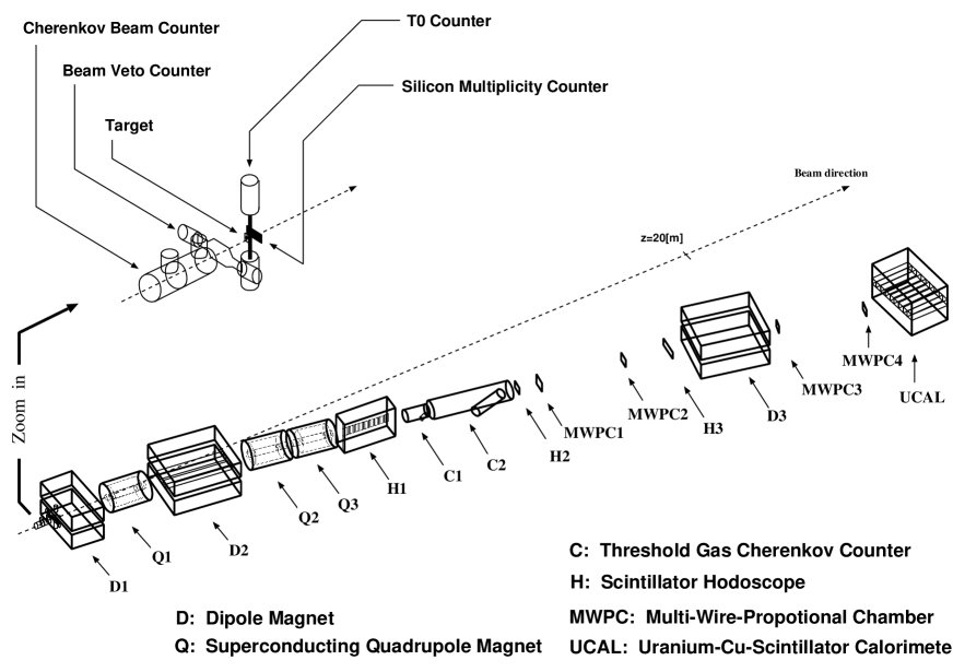
FIG. 1.: The NA44 experimental set-up.

FIG. 2.: The $p$ or $\bar{p}$ acceptance in y and $p_{T}$. The $\phi$ acceptance (not shown) decreases from $2\pi$ at $p_{T}$ = 0 to 0.012 at $p_{T}$ = 1.6 GeV/c.

FIG. 3.: Mass-squared distribution from Hodoscope 3 after pions have been vetoed by the Cherenkovs.

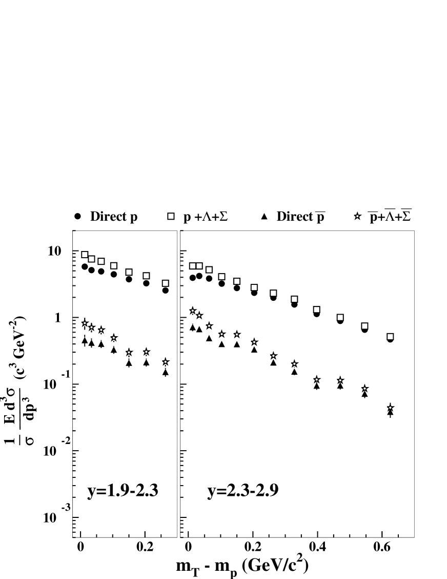
FIG. 4.: Invariant cross-sections as a function of $m_{T}-m_{p}$ for central $SPb$ collisions from RQMD, with (open symbols) and without (solid symbols) feed-down from weak decays.

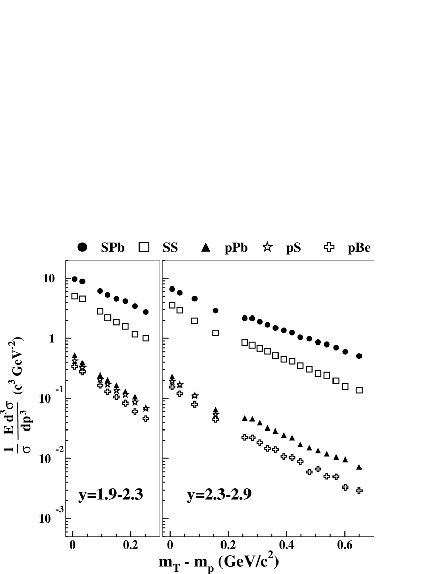
FIG. 5.: Invariant cross-sections for protons as a function of $m_{T}$ - $m_{p}$.

FIG. 6.: Invariant cross-sections for antiprotons as a function of $m_{T}$ - $m_{p}$.

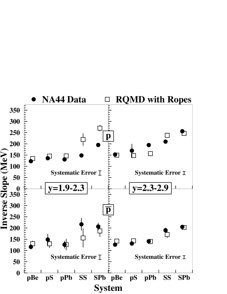
FIG. 7.: Inverse slopes of the transverse mass distributions for each system for data and RQMD. Statistical and systematic errors for the data are added in quadrature. The global systematic errors common to all systems (Table II) are shown by bars near the bottom right hand corner of each plot

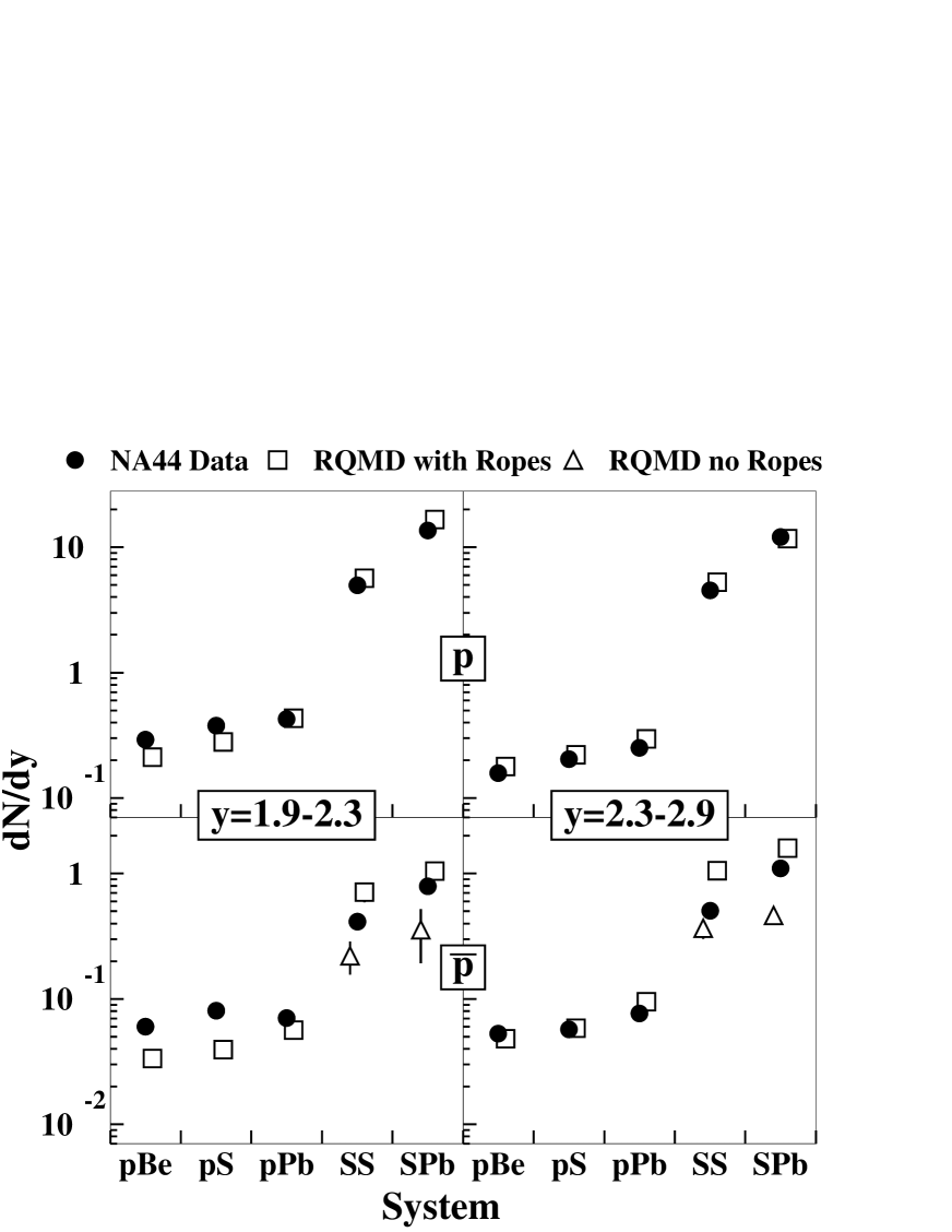
FIG. 8.: Rapidity densities (dN/dy) for each system for data and RQMD. Statistical and systematic errors for the data are added in quadrature.

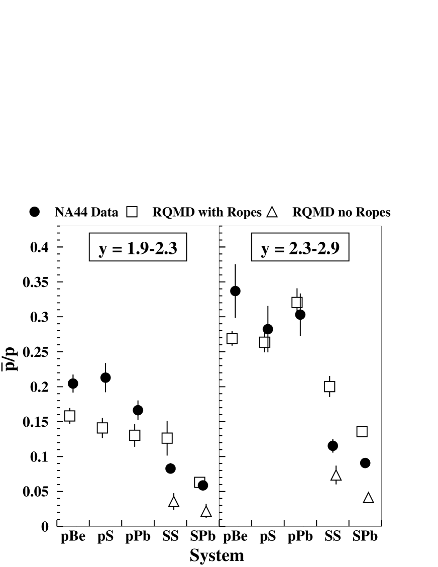
FIG. 9.: The integrated $\bar{p}$ to $p$ ratio for data and RQMD. Systematic and statistical errors have been added in quadrature. The value of the integrated ratio for $pp$ collisions [15] is $0.33\pm 0.13$.

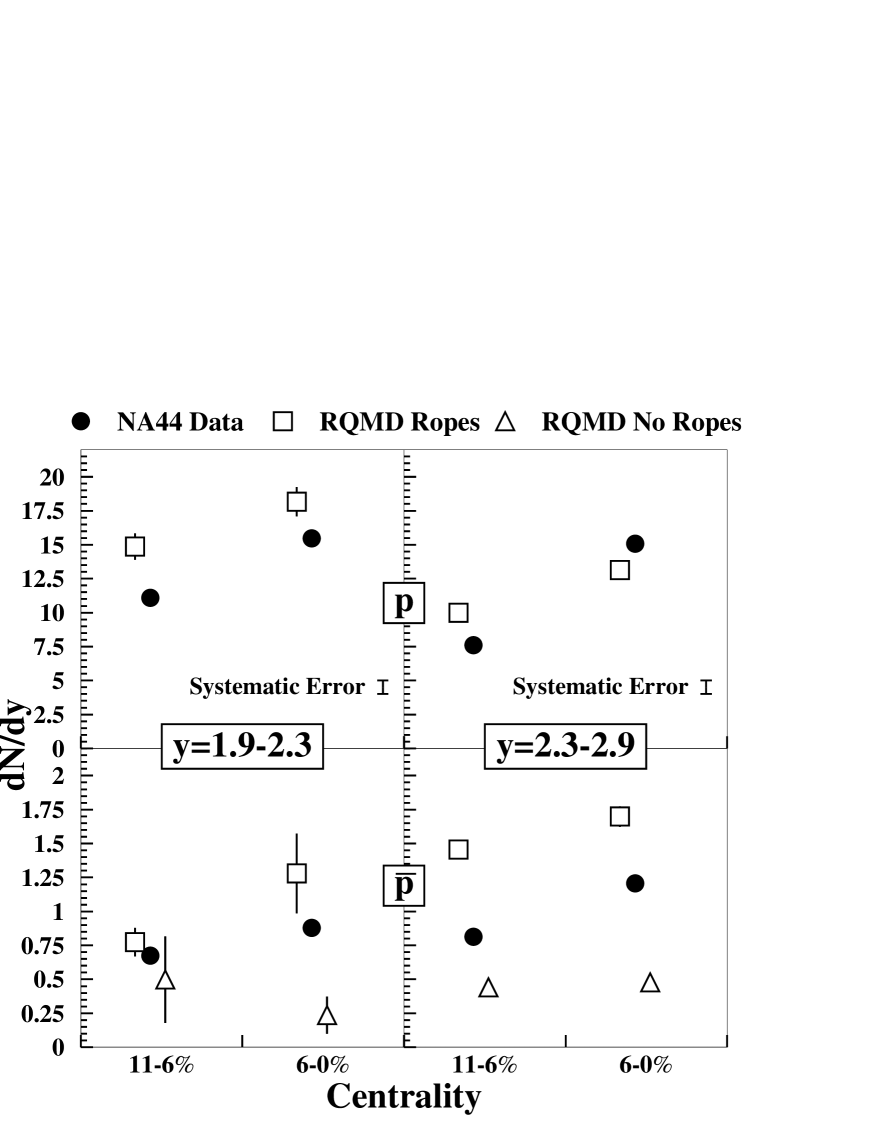
FIG. 10.: Proton and antiproton yields as a function of centrality for $SPb$ collisions. Statistical errors are shown for each point. The vertical bar shows the systematic error of 13.6% common to all of the data, see Table II. Also shown are the RQMD predictions for the same centrality selection.

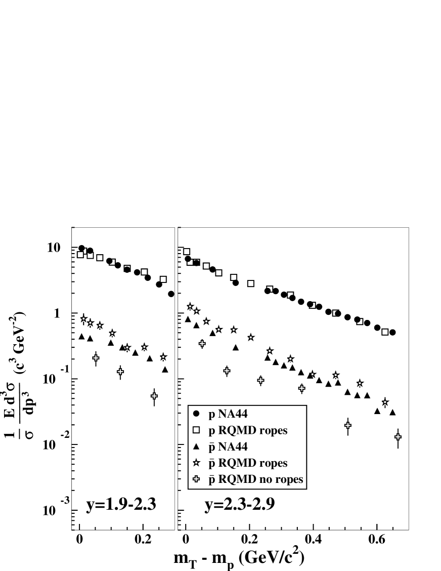
FIG. 11.: Invariant cross-sections as a function of $m_{T}-m_{p}$ for central $SPb$ collisions from data and RQMD. The RQMD distributions include the effect of feed-down from weak decays.

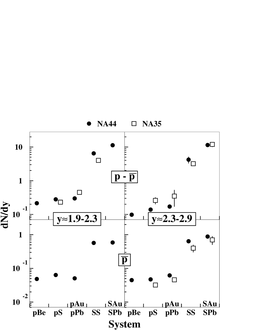
FIG. 12.: Comparison of NA44 and NA35, [16, 17], rapidity densities for $p-\bar{p}$ and $\bar{p}$. The $pA$ data were taken at 200 GeV/c for NA35 and 450 GeV/c for NA44. The NA44 $SS$ and $SPb$ data have been selected to have approximately the same centrality selection as the NA35 $SS$ and $SAu$ data, and all NA44 data have been corrected for feed-down using the factors in Table III. The NA35 $p-\bar{p}$ data are from the rapidity intervals 2.0-2.5 and 2.3-3.0 for both $SS$ and $SAu$; for $pA$ the NA35 rapidity ranges are 1.8-2.2 and the average of two bins covering rapidity 2.2-3.0. The NA35 $\bar{p}$ data are in the rapidity range 3-4.

REFERENCES

- [1] H. Sorge, H. Stöcker, W. Greiner, Nucl. Phys. A498 (1989) 567c.
- [2] U. Heinz, P.R. Subramanian, W. Greiner, Z. Phys A318 (1984) 247.
- [3] P.Koch, B. Müller, H. Stöcker, W. Greiner, Mod. Phys. Lett. A3 (1988) 737.
- [4] J. Ellis, U. Heinz, H. Kowalski, Phys. Lett. B233 (1989) 223.
- [5] K.S. Lee, M.J. Rhoades-Brown, U. Heinz, Phys. Rev. C 37 (1988) 1452.
- [6] S. Gavin, M. Gyulassy, M. Plümer, R. Venugopalan, Phys. Lett. B234 (1990) 175.
- [7] H. Sorge, A. V. Keitz, R. Mattiello, H. Stöcker, W. Greiner, Z. Phys. C 47 (1990) 629.
- [8] H. Sorge, M. Berenguer, H. Stöcker, W. Greiner, Phys. Lett. B289 (1992) 6.
- [9] N. Maeda et al., Nucl. Instr. Meth. A346 (1994) 132.
- [10] H. Beker et al., Phys. Rev. Lett. 74 (1995) 3340.
- [11] B. Nilsson-Almqvist and E . Stenlund, Comput. Phys. Comm. 43 (1987) 387.
- [12] H. Pi, Comput. Phys. Commun. 71 (1992) 173.
- [13] P. Foka, Strangeness in Hadronic Matter, AIP Conference Proceedings 340, Dec-1995, 182.
- [14] D. E. Greiner, Strangeness in Hadronic Matter, AIP Conference Proceedings 340, Dec-1995, 207.
-
[15]
K. Guettler et al.,
Phys. Lett. B64 (1976) 111;
K. Guettler et al., Nucl. Phys. B116 (1976) 77. - [16] T. Alber et al, Frankfurt preprint IKF-HENPG/6-94
- [17] T. Alber et al, Phys. Lett. B 366 (1996) 56.
- [18] I. G. Bearden et al., Phys. Lett. B388 (1996) 431.
- [19] D. E. Fields et al., Phys. Rev. C 52 (1995) 986.
- [20] K.S. Lee, U. Heinz, E. Schnedermann, Z. Phys. C48 (1990) 525.