Search for Exotic Strange Quark Matter in High Energy Nuclear Reactions

Abstract

We report on a search for metastable positively and negatively charged states of strange quark matter in Au + Pb reactions at 11.6 A GeV/c in experiment E864. We have sampled approximately six billion 10% most central Au + Pb interactions and have observed no strangelet states (baryon number A $<$ 100 droplets of strange quark matter). We thus set upper limits on the production of these exotic states at the level of $1-6\times 10^{-8}$ per central collision. These limits are the best and most model independent for this colliding system. We discuss the implications of our results on strangelet production mechanisms, and also on the stability question of strange quark matter.

, , , , , , , , , , , , , , , , , , , , , , , , , , , , , , , , , , , , , , , , , , , , , , , , ,

(The E864 Collaboration)

1 Introduction

All observed color singlet states involve either three quarks (baryons) or quark-antiquark pairs (mesons). However, the Standard Model which describes these states does not forbid the existence of color singlet states of more than three quarks (for example a bag of 18 quarks). It is known that such quark matter states made from only up and down quarks are less stable than normal nuclei of the same baryon number A and charge Z, since nuclei do not decay into quark matter. However, if such objects were made of three quark flavors, including strange quarks, they could gain stability from a reduction in the Fermi energy, despite the additional mass of the strange quark. Present theoretical understanding of strange quark matter states indicates that they are potentially metastable [1], and even possibly more stable than nuclear matter [2]. Due to the lack of theoretical constraints on bag model parameters and difficulties in calculating color magnetic interactions and finite size effects [3], the issue of the stability of strange quark matter is presently an experimental one.

There have been searches for strange quark matter in terrestrial matter [4], in cosmic rays and in astrophysical objects [5] (for a review see [6]). However, the most controlled investigation which attempts both production and detection to date is the search for strangelets in relativistic heavy ion collisions. Heavy ion collisions are a good environment to look for such states for three reasons. First, high energy heavy ion reactions are the only colliding system in the laboratory which produce significant strangeness and baryon number in a small volume from which a strangelet might be formed. Second, it is believed that in these collisions a phase transition to a quark-gluon plasma might occur. If a heavy ion collision results in the formation of hot quark matter it might then cool into a metastable state of cold strange quark matter. And last, because the accelerator is under the experimenters’ control, we can study a large number of reactions and set low sensitivity levels in the absence of observation.

2 Experiment

Experiment 864 at the Brookhaven AGS facility was specifically designed for the purpose of searching for strangelets. Strangelets are expected to have a unique experimental signature of a low charge to mass ratio (below the range of known nuclear isotopes) due to the roughly equal numbers of up, down and strange quarks (charge +2/3, $-$1/3, and $-$1/3). The experiment identifies secondary particles produced in Au + Pb collisions at 11.6 GeV/c per nucleon by measuring their masses and charges. The experiment has a large geometric acceptance and can operate at high interaction rates up to $10^{6}$ collisions per one second beam spill. These two features allow the experiment to achieve a high level of sensitivity.

2.1 Apparatus

The apparatus is shown in Fig. 1. A collimated beam of Au ions (shown as an arrow) passes through a quartz plate Cerenkov counter. This beam counter is able to deliver timing information for each ion with a resolution of $\sigma_{t}\approx 100$ ps at incident rates up to $10^{7}$ ions per one second spill. This information is used as the starting time our velocity measurements. There are veto counters to reject beam particles outside our profile, upstream beam interactions, and events with two or more incident Au ions. The target is a Pb disk and 30% of an interaction length for Au. Non-interacting Au ions and beam fragments with low transverse momentum are contained in an aluminum and steel vacuum chamber (shown in the elevation view) to reduce interactions in air which might shower secondary particles into the downstream spectrometer.

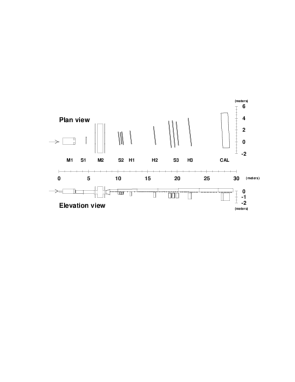
Figure 1: Experiment 864 detector layout in plan and elevation view. The incident beam on the Pb target is shown as an arrow. The two dipole magnets are labeled as M1 and M2. Also shown are the straw stations (S1, S2, S3), the three time-of-flight hodoscopes (H1, H2, H3) and the hadronic calorimeter (CAL). One can see the full extent of the vacuum chamber in the elevation view.

Downstream of the target are two dipole magnets (M1 and M2). The straw tube tracking detector (S1) inside the vacuum chamber between the two magnets was not used in the analysis presented here. Au ions which interact in the target produce secondary particles which, after passing through the two magnets, may exit the vacuum chamber through a thin window. These secondaries then traverse the remainder of the spectrometer below the vacuum chamber. Particles must have a downward vertical angle of at least $-$17.5 milliradians to exit through the window.

Those secondary particles within the acceptance are tracked using two stations of straw tubes (S2 and S3) and three time-of-flight hodoscopes (H1, H2 and H3). Each of the time-of-flight hodoscopes consists of 206 plastic scintillator slats read out by two photo-multiplier tubes (one at the top and one at the bottom). The scintillators have 45 degree diamond mill finished ends to reflect the light from the scintillator through a 90 degree bend into a cylindrical lucite light guide. This 90 degree bend allows the detector to be placed as close to the vacuum chamber as possible, thus extending our acceptance closer to zero degrees in the vertical direction. The hodoscopes give three independent measurements of the particle charge via energy loss $dE/dx$. Also each plane yields time-of-flight from the mean time of the two photo-multiplier tubes with a resolution of $\sigma_{t}\approx$ 120-150 ps. The straw tube detectors are used to improve a track’s spatial resolution. Each straw tube station is made up of three planes ($x,u,v$), with one oriented in the vertical and the others at $\pm$ 20 degrees relative to vertical. The straws are 4 mm diameter tubes and are stacked in a doublet configuration for each plane, eliminating possible gaps in the detector.

At the end of the spectrometer is a spaghetti design hadronic calorimeter. The calorimeter consists of 754 towers with dimension $\rm{10~{}cm\times 10~{}cm\times 117~{}cm}$. The calorimeter is approximately five hadronic interaction lengths deep. Each tower is constructed from grooved lead sheets with scintillating fibers approximately collinear to the incident particle trajectories. The ratio of lead to fiber is chosen to approximately compensate the calorimeter energy responses for hadronic and electro-magnetic showers. This fiber configuration leads to an excellent timing resolution $\sigma_{t}\approx 400$ ps for hadronic showers. The energy resolution for hadrons has been determined to be 6% + 34%/$\sqrt{E}$, where $E$ is the energy deposited in units of GeV [7]. More details on the calorimeter performance are given in Ref [8].

2.2 Trigger

The data acquisition system can record approximately 1500 events per one second spill over a four second duty cycle, and thus in order to sample the interaction rate we have implemented two triggers. The probability for strangelet production is expected to be significantly increased in the most central collisions [9]. Thus, a low level trigger selects approximately the 10% most central (low impact parameter) Au + Pb interactions. This selection is made using a four fold segmented scintillation counter covering forward angles from 16.6 to 45.0 degrees [10]. Interactions producing pulse heights in the 10% highest fraction are selected.

The second trigger is a high mass trigger which is used to select events with possible strangelet candidates and reject events with only normal hadrons in our spectrometer. The calorimeter measures the particles’ kinetic energy and time-of-flight (which is easily related to the velocity $\beta$). We have constructed a trigger connected to each calorimeter tower which has a programmable look-up table of accept values. Shown in Fig. 2 is a Monte Carlo generated kinetic energy and time-of-flight distribution at the front face of the calorimeter (without detector effects). The upper band is simulated strangelets with A = 5 and Z = $-$1. The lower band is simulated neutrons and protons striking the calorimeter. An example of a trigger curve is shown in the figure. Any event in which at least one tower measures an energy and time-of-flight above the curve would be recorded. There is a minimum time-of-flight cut component to the trigger such that we only accept candidates with rapidity approximately $y<2.2$. In the experiment, the distributions are significantly blurred by finite time resolution, single tower energy sampling, and energy resolution. However, we were able to program the trigger such that only 2% of ordinary central interactions fire the high mass trigger, while maintaining greater than 90% trigger efficiency for strangelets of mass greater than 5 GeV/c².

Figure 2: Results from Monte Carlo simulation of the kinetic energy versus the time-of-flight at the front face of the calorimeter are shown for nucleons (neutrons and protons) and for strangelets (baryon number A=5 and charge Z=$-$1). The points assume perfect timing and energy information. Data from the experiment have significant blurring of the distributions due to limited energy sampling and detector resolutions. An example high mass trigger cut is shown as a solid line.

2.3 Data Sets

The results discussed in this paper are from data taken in the fall of 1995. For these studies we operated the spectrometer at two different magnetic field configurations. We recorded approximately 85 million events at what we refer to as the “$-$0.75T” field setting which optimizes the acceptance for negatively charged strangelet states while sweeping out copiously produced hadrons (kaons, protons, etc.). We also took approximately 27 million events at the “+1.50T” field setting which optimizes the acceptance for positively charged strangelet states. Each data set was taken using both the centrality trigger requirement and the high mass trigger. We have searched only for positively charged states in the “+1.50T” data sample; however, in the “$-$0.75T” data, due to the larger number of events and the lower magnitude of the field, there is significant sensitivity to positively as well as negatively charged states. We combine the final results from each data sample to calculate our experimental limits.

3 Analysis

In this section, we present the details of the strangelet search analysis. A complete description of the analysis of the “$-$0.75T” data set may be found in [7]. There are some differences in the analysis of the “+1.50T” data set due to differences in detector occupancies and background sources, not detailed in this paper. Complete details of the “+1.50T” data set may be found in [11].

3.1 Tracking

We identify charged particle tracks which have consistent hits in the straw tube chambers and the three time-of-flight hodoscopes. After all hits have been associated with a given track, we make a global fit using all hit information to determine the particle’s trajectory. From the trajectory of the track in the bend plane of the magnetic field, we determine the particle’s rigidity ($R=p/Z$) assuming the track originated at our production target. The charge of the particle is measured from energy deposition ($dE/dx$) in each of the three hodoscope planes. The velocity $\beta$ is calculated from the path length of the track and hodoscope time-of-flight information. The mass of the track can now be calculated.

$$m={{R\times Z}\over{\gamma\beta}}$$ (1)

Thus, for each track candidate we have a measure of the mass and charge. At the first stage in analysis, we save all events with possible strangelet candidates in the rapidity range $1.0<y<2.2$ with mass greater than 5 GeV/c² and any charge Z=$\pm$1,$\pm$2. The only known particles expected within this sample are ⁶He and ⁸He isotopes. We find that only a small percentage (1-2%) of the recorded events contain candidates.

In doing a sensitive search for new particle states, it is critical to have significant redundancy in various measurements in order to reduce possible background which might yield false signals for strangelets. The first level of redundancy is in the tracking system described above. Through multiple tracking measurements, we over determine the particle trajectory in space and time. We have fit to the track velocity and horizontal and vertical path, and the $\chi^{2}$ value from each fit is examined. Known hadronic species measured in the same data sample (antiprotons, deuterons, ³He isotopes) show good agreement with the theoretical $\chi^{2}$ calculations for the correct number of degrees of freedom. This agreement gives us confidence that we understand the alignments, calibrations and resolutions of the tracking detectors. We apply track quality cuts on these $\chi^{2}$ values with known efficiencies for “good” particles to further reject possible background tracks reconstructing as strangelets. The $\chi^{2}$ cuts are determined to be  80% efficient (as verified with identified antiprotons). When the cuts are applied to the set of strangelet candidates, only approximately 20% of the candidates remain. This low percentage indicates that the majority of the candidates are background, and thus have significantly worse track quality.

From the “$-$0.75T” data sample, the distribution of reconstructed masses from tracking for Z=$-$1 candidates surviving track quality cuts is shown in Fig. 3. A prominent peak containing approximately 50,000 antiprotons is seen with an exponential tail of higher mass candidates. The antiproton mass is at the Particle Data Book value with a mass resolution of approximately $\Delta m/m\approx 4$%, as expected from our time-of-flight and momentum resolutions. There are approximately 20,000 remaining Z = $-$1 candidates with mass greater than 5 GeV/$c^{2}$ (as shown in the figure). Also, there are a few hundred Z = +1 candidates with mass greater than 5 GeV/$c^{2}$ from the “+1.50T” data sample. There are no Z = $-$2 candidates and only a few Z = +2 candidates with masses beyond the mass for ⁶He.

Figure 3: The track reconstructed mass distribution for Z=$-$1 candidates from the full “$-$0.75T” data sample.

3.2 Background Sources

There is a known source of background in our spectrometer which can create high mass candidates from track reconstruction. A neutron leaving the target can pass undeflected through a portion or all of the magnetic field region and then undergo an inelastic reaction in the vacuum exit window, the straw chamber in vacuum (S1), air, etc., emitting a forward going proton. The proton creates a charged particle track in all of the downstream tracking detectors. The track may have a reasonable velocity, $\beta$, but the reconstructed rigidity can be large, since the neutron trajectory did not bend in the magnetic field. These erroneous high rigidity measurements can yield high mass candidates. We have done extensive Monte Carlo simulations of this background reaction [12]. Despite the fact that the resulting particle in the spectrometer is a proton, the track can also mimic a Z=$-$1 particle since the track results from a neutron (whose trajectory is unaffected by the magnetic fields).

This background process results only in Z=$\pm$1 candidates, which explains the significantly lower number of Z=$\pm$2 candidates. Also, there will be some inconsistency in the tracking fits for these candidates, since the inelastic interaction has some kink angle between the incoming neutron and outgoing proton. This feature explains the low acceptance for the $\chi^{2}$ cut for these candidates. However, for some of these background reactions the track quality appears good and the tracking system is fooled.

3.3 Hadronic Calorimeter

The calorimeter makes an second measurement of the particle mass completely independent of the magnetic field region:

$$m={{KE}\over{\gamma-1}}$$ (2)

where KE is the kinetic energy of the particle and $\gamma$ is the relativistic factor. The tracks resulting from the background process described above should reconstruct with the mass of a proton in the calorimeter. If the candidates are real strangelets, they should have a significantly higher energy deposit yielding a consistent tracking and calorimeter mass.

Each of the candidate tracks is projected to the front face of the calorimeter. If there is a local energy maximum in the calorimeter (peak tower) within one tower of the projected position, we associate the charged particle track with that particular calorimeter shower. The calorimeter energy scale has been normalized such that, on average, the sum of energy deposited in a three by three array of towers surrounding and including the peak tower is equal to the charged particle’s total kinetic energy. Thus, for each candidate we compute the total kinetic energy from the nine tower sum.

We require that the peak tower time-of-flight agrees with the projected time from the hodoscopes within $\pm$ 2 ns. If this agreement is met, since the hodoscope time resolution is significantly better than the calorimeter resolution, we calculate the velocity $\beta$ using the three hodoscopes only. It should be noted that this calculation does not use the assumed time at the target.

Before proceeding further, since real strangelets are expected to deposit significantly more energy in the calorimeter than “fake” strangelets (which are really protons striking the calorimeter), it is critical to eliminate calorimeter showers which have energy contamination from other particles. Various cuts are applied to the calorimeter information to remove contaminated energy showers. Cuts are placed on the time agreement of the eight side towers and the central position of the cluster with respect to the position projected from tracking. We also require that there be no other energy peaks in the towers surrounding the shower of interest. The cuts maintain good efficiency for “real” strangelet showers, while rejecting contaminated ones. The timing and energy cuts used for the “+1.50T” data set are slightly different, on account of differences in total particle occupancy and overall background levels.

In using the calorimeter, we assume that the strangelet has a hadronic shower in the calorimeter. We have assumed that light strangelets will fragment in their first one or two inelastic collisions into their constituent baryons (and resulting mesons). We have studied the calorimeter response to light nuclei such as ⁴He. Shown in Fig. 4 is the distribution of calorimeter energies (measured in the peak tower only) from identified alpha particles. Also shown is the combination of four separate proton showers with similar kinetic energy per nucleon to the alpha showers shown. The agreement is quite good and gives us confidence in our picture of the interaction of multi-baryonic objects in the calorimeter.

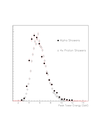
Figure 4: The distribution of calorimeter measured energy (in the peak tower only) for ⁴He particles. These ⁴He have fired the high mass trigger. The ⁴He have a kinetic energy of approximately 11 GeV, with  50% of the energy expected to be deposited in the peak tower. Also shown in open circles is the energy distribution of four independent proton showers summed together with similar kinetic energy per nucleon.

3.4 Mass versus Mass

For all candidates with associated uncontaminated calorimeter showers, we plot the tracking mass versus the calorimeter mass. A distribution of the tracking mass versus the calorimeter mass for all Z=$-$1 candidates is shown in Fig. 5. We have plotted the low mass region as a contour plot to show the prominent antiproton peak. It is observed that the antiproton mass reconstructed in the calorimeter using Eq. 2 is higher than the tracking mass. This difference is expected because antibaryons deposit not only their kinetic energy in the calorimeter, but also twice the mass energy from the annihilation. If we recompute the antiproton mass from the calorimeter, removing the expected annihilation energy, then the tracking and calorimeter masses are in good agreement. All candidates with a tracking mass above 5 GeV/c² are shown as larger boxes.

Figure 5: The plot shows Z=$-$1 particle candidates measured masses from tracking versus calorimeter reconstructed masses. Shown as a contour plot is the mass region from 0.0-5.0 GeV/c² with a clear peak of antiprotons. All candidates with tracking mass greater than 5 GeV/c² are shown as boxes.

In the mass range $5-10~{}\rm{GeV/c^{2}}$ the calorimeter mass is required to agree with the tracking mass within $-1.0\sigma$ and $+3.0\sigma$, where $\sigma$ is the $RMS$ mass resolution from the calorimeter. This mass resolution is dominated by the energy resolution of the calorimeter. There are no candidates which meet this requirement in this mass range.

Above tracking mass of 10 GeV, the agreement requirement is loosened. The calorimeter has been shown to have a linear energy response up to at least 12 GeV [8], but at some larger energy the photo-multiplier gains saturate and this linearity is violated. Additionally, the amplitude-to-digital converters, ADC’s, have a finite range only extending up to approximately 40 GeV per tower in measured energy. Therefore high mass candidates which deposit a large amount of energy may reconstruct a lower calorimeter mass than expected. Thus, we want to be careful about the calorimeter mass required for high mass candidates. There is only one potential candidate with tracking mass greater than 10 GeV/c². This candidate is shown in Fig. 5 and has a tracking mass of 15.2 GeV/c² and a calorimeter mass of 7.8 GeV/c². The kinetic energy from the tracking information is 61 GeV, while the calorimeter measured energy is only 21 GeV. The peak calorimeter tower measured only 11.3 GeV, below the energy range where the gains might saturate. Therefore, this one potential candidate is considered background.

There have been interpretations of cosmic ray “Centauro” type events as resulting from heavy strangelets (A $>>$ 10) which penetrate through the Earth’s atmosphere [13, 14]. The strange quark droplets might have a density significantly greater than normal nuclear matter density, and thus have a smaller inelastic cross section than a comparable nucleus. However, any strangelet in our experiment strikes five hadronic interaction lengths of lead (for a strangelet with the geometric size of a proton), and we expect a negligible probability of significant energy leakage out the back of our calorimeter.

Similar analysis for charge Z = +1 from the “+1.50T” data reveals no strangelet candidates after consideration of the calorimeter and tracking information. As stated before, there are no Z = $-$2 candidates, even before considering the calorimeter response. The distribution of charge Z = +2 candidates from the “+1.50T” data sample is shown in Fig. 6. The mass range below 5 GeV/c² is shown as a contour plot where one can see clear peaks for ³He and ⁴He isotopes. All points above tracking mass of 5 GeV/c² are shown as boxes. There are no consistent candidates above A=6. From the two field settings, there are approximately 50 ⁶He nuclei measured within $\pm$ 0.6 units of mid-rapidity. These nuclei are believed to be not from beam or target fragments, but rather from the coalescence of separate nucleons [15]. This is the first significant measurement of A=6 coalescence yields at these energies, which represents a true six particle correlation. We will discuss the importance of these yields in the final section of this paper.

Figure 6: The scatter plot is Z=+2 particle candidates measured mass from tracking versus calorimeter reconstructed mass. Shown as a contour plot is the mass region from 0.0-5.0 GeV/c² with peaks from ³He and ⁴He. All candidates above this mass are shown as squares. The only particles in this mass range with consistent tracking and calorimeter masses are identified as ⁶He isotopes.

In summation, there are no remaining consistent candidates for Z=$\pm$1,$-$2 above mass 5 GeV/c², and Z=+2 above mass 6 GeV/c². Thus, we use this information to set upper limits on the production of strangelet states.

4 Production Limits

In order to relate the null result to overall production limits, we need to calculate the fraction of possible strangelets we would have measured. The acceptances and efficiencies vary for different strangelet species and depend on the expected kinematic distribution of strangelets.

Strangelets, since they are yet to be discovered, have an unknown momentum distribution. We assume the following production model:

$${{d^{2}N}\over{dydp_{t}}}\propto p_{t}e^{-{{2p_{t}}\over{<p_{t}>}}}e^{-{{(y-y_{NN})^{2}}\over{2\sigma_{y}^{2}}}}$$ (3)

We further assume that the mean transverse momentum $<p_{t}>=0.6\sqrt{A}$ GeV/c, where A is the mass of the strangelet in baryon number, and $\sigma_{y}$ = 0.5 is the width of a Gaussian rapidity distribution centered at mid-rapidity ($y_{NN}=1.6$). The rapidity and transverse momentum distributions are assumed to be uncorrelated. Shown in Fig. 7 is the geometric acceptance for a charge one, A=20 strangelet as a function of rapidity and transverse momentum. The coverage extends over a wide range of rapidity and $p_{t}$, thus making the experimental results relatively insensitive to the expected distribution. It should be noted that we do not have acceptance extending to $p_{t}=0$ due to the physical constraint of the vacuum chamber. For example, a mid-rapidity A=20 strangelet must have at least 800 MeV/c (40 MeV/c per nucleon) of transverse momentum to be detected in the downstream spectrometer.

Figure 7: The geometric acceptance for strangelets (A=20, Z=$-$1) at the “$-$0.75T” field setting is shown as a function of rapidity and transverse momentum. The inner most and outer most contour lines surround acceptance values in excess of 25% and 3%, respectively.

The final strangelet limits are quoted as 90% confidence level upper limits in 10% most central Au+Pb interactions at 11.6 A GeV/c. The limit is given as:

$$90\%\rm{C.L.}~{}=~{}{{N_{Poisson}}\over{N_{sampled}}}~{}~{}{{1}\over{\epsilon_{accept}\times\epsilon_{tracking}\times\epsilon_{calorimeter}\times\epsilon_{trigger}}}$$ (4)

where the 90% confidence level limit from Poisson statistics is $N_{Poisson}=2.30$ and $N_{sampled}$ is the total number of events sampled. The various efficiencies $\epsilon$ are described below.

The efficiencies vary with strangelet species (A,S) and with the production model, but typical values are given below. The overall geometric acceptance $\epsilon_{accept}$ is approximately 8%. The tracking efficiency $\epsilon_{track}$ including track quality cuts is approximately 75%. The calorimeter contamination cut efficiency $\epsilon_{calorimeter}$ varies over quite a range depending on the incident particle occupancy from 40-80%. Finally, the trigger efficiency $\epsilon_{trigger}$ values are quite high, in the range of 90-100%. We have calculated these efficiencies using a full GEANT simulation of the experiment including the magnets, vacuum chamber, detectors, etc. We have used detector survey data as input for the various detector geometries. We use this simulation for the calculation of geometric acceptance and single particle tracking efficiency. We determine the efficiency of each detector (for example due to small gaps between scintillator slats in the hodoscopes) by using the data to find tracks without using a given detector and then checking for a consistent hit in that detector. In order to determine the multi-track efficiencies and calorimeter shower cut efficiencies, we have taken Monte Carlo detector hit information (simulating the measured detector responses), overlayed these hits with real experimental data, and processed the results through our tracking and shower analysis.

The upper limits for the two data sets combined are shown in Fig. 8. The final limits do not depend significantly on the production model (at the level of a factor of two) since the experiment is sensitive over a broad range of momentum space. The final limits are also relatively independent of the strangelet mass.

Figure 8: Shown are the 90% confidence level upper limits per 10% most central Au + Pb collision for negatively and positively charged strangelet states as a function of strangelet mass. The solid lines are for Z=$\pm$1 and the dashed lines are for Z=$\pm$2.

These limits are for metastable strangelets with proper lifetimes on the order of $\tau\geq 50$ ns. If the lifetime of the strangelet is less than 50 ns, the sensitivity drops significantly. Shown in Fig. 9 is the lifetime dependence of our upper limits. The lifetime dependence is calculated using a 100 ns flight time (approximately the time-of-flight to the calorimeter), a relativistic factor $\gamma=2$, and an upper limit of $2\times 10^{-8}$ per central interaction for lifetimes significantly greater than 50 ns.

Figure 9: Shown are the 90% confidence level upper limits per 10% most central Au + Pb collision for negatively and positively charged strangelet states as a function of strangelet lifetime.

5 Other Experimental Results

There have been previous searches for charged strangelets in relativistic heavy ion experiments. To date no experiment has published results indicating a clear positive signal and so all have set production upper limits. This statement excludes $H^{0}$ dibaryon results for which there are experimental observations [16, 17], but no definitive conclusions. Earlier searches for charged strangelets were performed using Si beams at the BNL-AGS by experiments E814 [18] and E858 [19], and using S and Pb beams at higher energies at the CERN-SPS by experiment NA52 [20]. All have published null results. The production potential (probability for strangelet formation) may be quite different for smaller colliding systems using Si and S beams or systems at significantly higher beam energy (which produce systems with a lower baryon density). Therefore, it is difficult to compare these experimental limits with the present results.

There are two experiments at the BNL-AGS which have set limits in Au + Au (Pt) collisions. Both experiments E878 [21] and E886 [22] set limits per minimum bias collision, which we need to relate to our limits in the 10% most central collisions. If we assume that 50% of all strangelets are produced in the 10% most central collisions (which one might roughly expect given the coalescence calculations in [9]), then our limits in central collisions should be divided by a factor of five to convert to limits per minimum bias collision. This results in E864 limits at approximately $4\times 10^{-9}$ per minimum bias collision. Experiments E878 and E886 set limits in minimum bias collisions for negatively charged strangelets at approximately $5\times 10^{-9}$ and $1\times 10^{-8}$ respectively, and for positively charged strangelets at approximately $5\times 10^{-6}$ and $1\times 10^{-7}$ respectively.

It is critical to note that both E886 and E878 are focusing spectrometer experiments which operate with maximum rigidity settings of 2 GeV/c/Z and 20 GeV/c/Z, respectively. Since the production of strangelets is expected to be peaked at mid-rapidity (corresponding to a momentum per nucleon of 2 GeV/c), these rigidity limitations make these experiments relatively insensitive to strangelets with masses significantly greater than 10 GeV/c². Thus, in the mass range 10-100 GeV/c², the limits set in this paper represent by far the best limits to date.

6 Constraining Production Models

Ideally, we would like to use these limits to make a fundamental statement about the stability of strange quark matter. We would like to constrain the bag model parameters to eliminate values which predict metastable strangelets in this mass range. Even within the framework of the bag model, there is a correlated set of parameters which have not been fully explored theoretically as regards the strangelet states the model would predict. Some regions of this parameter space, of course, have been worked out and as noted were the motivation for this experiment. In addition, the mechanisms by which strangelets would be produced in heavy ion collisions are not well known and so one must consider different production models. In the analysis below, we examine the different production models and are able to establish interesting and useful constraints, in some cases, on the joint hypothesis regarding the models and particular strangelet states.

6.1 Plasma models

The most optimistic mechanism for the production of strangelets involves the formation of a quark-gluon plasma [23]. However, this scenario is also the most difficult in which to produce reliable theoretical calculations as to the exact rate of strangelet production. If a quark-gluon plasma is formed in some of the heavy ion collisions studied, the plasma is expected to have a large net baryon density – rich in $u$ and $d$ quarks and poor in $\overline{u}$ and $\overline{d}$ quarks. This hot quark system cools via the emission of mesons. Since it is easier for antistrange quarks to pair up with $u$ and $d$ quarks in $K^{+}$ ($u\overline{s}$) and $K^{0}$ ($d\overline{s}$), as opposed to strange quarks pairing with $\overline{u}$ and $\overline{d}$ quarks, the hot plasma gains net strangeness. As the plasma cools it may form a droplet of cold strange quark matter which might be metastable and be measurable in our experiment.

Our experiment cannot explicitly rule out any one of the steps required in this process: (1) QGP formation, (2) strangeness distillation, and (3) metastable strangelet states. However, we can state that in approximately $10^{8}$ central collisions, the combination of these three steps does not occur.

$$\rm{Probability(1)\times Probability(2)\times Probability(3)<10^{-8}}$$ (5)

For example, if one believed that a QGP is formed in 1 out of 10,000 central Au+Pb collisions, then the probability of this QGP forming a metastable charged strangelet is less than 0.01%.

There are specific predictions on production rates of strangelets assuming a QGP phase transition. Crawford et al. calculate negatively and positively charged strangelet production levels in heavy ion collisions [24]. The model assumes that a quark-gluon plasma is formed in every 10% most central collision and determines how often a strangelet of given mass and charge is distilled out. Their predictions for charged strangelets of mass 10-20 GeV/c² from minimum bias Si+Au collisions are in the range of $4\times 10^{-11}$ to $8\times 10^{-8}$. One might expect higher production rates in central Au + Pb collisions. Our limits eliminate some of the predictions; however, the calculations have many rough assumptions and should not be viewed as exact within orders of magnitude.

6.2 Coalescence Models

A very different production mechanism for strangelets is via the coalescence of strange and non-strange baryons. In the QGP scenario, a large fraction of the colliding system may form a bubble of hot quark matter which may cool into a strangelet. Thus, the strangelet could have quite a large mass (A $>$ 15). In a coalescence picture, after the colliding system has expanded significantly, interactions between particles become less frequent until eventually the particles are free streaming (freeze-out). At the point of freeze-out baryons which are close to each other in configuration space and momentum may fuse together to form nuclei or possibly hypernuclei. Most hypernuclei are expected to have lifetimes on the order of the $\Lambda$ particle and thus would decay before traversing our spectrometer. However if a strangelet state of similar quantum numbers (A, S) were more stable than the hypernucleus, the nuclear state might act as a doorway to the strange quark matter state.

One can make relatively reliable coalescence rate calculations, which can be checked with nuclear isotope yields. In the paper of Baltz ${\it et~{}al.}$, the authors predict a rate of ${}^{7}_{\Xi^{0}\Lambda\Lambda}{\rm{He}}$ at 3-7$\times 10^{-8}$ per central Au + Au collision [9], while our sensitivity for a strangelet state with the same quantum numbers is $6\times 10^{-8}$. One might thus conclude that we are testing limits within the coalescence model at the level of A = 7 and $|S|=4$. However, recent results from our experiment for measured light nuclei indicate that the calculations in [9] overestimate the experimentally measured yield of light nuclear isotopes like ³He and ⁴He [25]. Also, in the data sets discussed in this paper, we observe a significant number of ⁶He isotopes, but no ⁸He states (note that ⁷He is unstable on the lifetime scale required to be measured in our experiment). Thus, we have roughly reached a coalescence sensitivity of A=7 and $|S|=0$. For each coalesced baryon, the penalty for changing a non-strange baryon to a strange baryon is estimated to be approximately 0.2 [9]. Therefore, the experiment is roughly sensitive to states with

$$|A|+0.5\times|S|~{}~{}~{}<~{}~{}~{}7$$ (6)

We are beginning to address the coalescence production of strangelets for relatively light states. If we had observed a heavy strangelet state ($A>10$), it would have been good evidence for the plasma distillation mechanism, since this mass range is beyond what one would expect from coalescence.

7 Conclusions

In experiment 864, using data taken in the fall of 1995, we have sampled nearly six billion central Au + Pb collisions at the BNL-AGS. Through the use of significant redundant tracking measurements and calorimetry, we find no consistent candidates for new states of strange quark matter. This represents the lowest and most significant limit to date in relativistic heavy ion collisions at these energies. From data taken in the winter of 1997 and to be taken in 1998, we will either extend these limits by approximately an order of magnitude or possibly discover strangelets.

8 Acknowledgments

We acknowledge the efforts of the AGS and Tandem staff in providing the Au beam for the experiment. This work was supported by grants from the Department of Energy (DOE) High Energy Physics Division, DOE Nuclear Division, the National Science Foundation, and the Istituto Nationale di Fisica Nucleare of Italy (INFN).

Finally, we would like to record here the respect, affection, and appreciation which our collaboration shares for our late colleague, Carl Dover. It should be noted that this experiment, E-864 at the BNL AGS, owed a great deal to Carl’s insight and knowledge. He was instrumental in both the original conception of the experiment and in its design and scope. His wisdom, and his friendship will be sorely missed.

References

- [1] E. Farhi and R.L. Jaffe, Phys. Rev. D 30, 2379 (1984).
- [2] E. Witten, Phys. Rev. D 30, 272 (1984).
- [3] J. Schaffner et al., Phys. Rev. Lett. 71, 1328 (1993); E.P. Gilson and R.L. Jaffe, Phys. Rev. Lett. 71, 332 (1993); J. Madsen, Phys. Rev. Lett. 70, 391 (1993).
- [4] T.K. Hemmick et al., Phys. Rev. D41, 2074 (1990).
- [5] C. Alcock and A. Olinto, Ann. Rev. Nucl. Part. Sci. 38, 161 (1988).
- [6] S. Kumar, in Physics and Astrophysics of Quark-Gluon Plasma, edited by B. Sinha, Y.P. Viyogi, and S. Raha (World Scientific, Singapore, 1994).
- [7] J.L. Nagle, Ph.D. Thesis, Yale University (1997).
- [8] Experiment E864: K.N. Barish et al., submitted to Nucl. Inst. Methods (1997).
- [9] A.J. Baltz et al., Phys. Lett. B 325, 7 (1994). Table II, column 2 (central Au + Au collisions), Equation (5) of this paper has a numerical error which we have corrected here.
- [10] P. Haridas et al., Nucl. Inst. Meth. A385, 412 (1997).
- [11] S.D. Coe, Ph.D. Thesis, Yale University (1997).
- [12] K.N. Barish, Ph.D. Thesis, Yale University (1996).
- [13] J.D. Bjorken and L.D. McLerran, Phys. Rev. D20, 2353 (1979).
- [14] Brazil-Japan collaboration, in Proceedings of the Plovdiv International Conference on Cosmic Rays, 1977, edited by B. Betev (Bulgarian Academy of Science, Sofia, 1977), Vol. 7, p 208.
- [15] J.L. Nagle et al., Phys. Rev. C53, 367 (1996).
- [16] Experiment E810: R. Longacre et al., Nucl. Phys. A590, 477c (1995).
- [17] Experiment E888: J. Belz et al., Phys. Rev. Lett. 76, 3277 (1996).
- [18] Experiment E814: F.S. Rotondo et al., Nucl. Phys. B 24B, 265 (1991), J. Barette et al., Phys. Lett B 252, 550 (1990).
- [19] Experiment E858: A. Aoki et al., Phys. Rev. Lett. 69, 2345 (1992).
- [20] Experiment NA52: G. Ambrosini et al., Nucl. Phys. A610, 307c (1996). G. Appelquist et al., Phys. Rev. Lett. 76, 3907 (1996). K. Borer et al., Phys. Rev. Lett. 72, 1415 (1994). F. Stoffel et al., APH N.S., Heavy Ion Physics (1996) 429-434 (1996).
- [21] Experiment E878: D. Beavis et al., Phys. Rev. Lett. 75, 3078 (1995).
- [22] Experiment E886: A. Rusek et al., Phys. Rev. C 52, 1580 (1995). A. Rusek, Ph.D. Thesis, University of New Mexico (1996).
- [23] C. Greiner, P. Koch, and H. Stocker, Phys. Rev. Lett. 58, 1825 (1987); C. Greiner, D. Rischke, H. Stocker, and P. Koch, Z. Phys. C 38, 283 (1988); C. Greiner and H. Stocker, Phys. Rev. D 44, 3517 (1991).
- [24] H. Crawford et al., Phys. Rev. D 45, 857 (1992).
- [25] J.K. Pope for the E864 Collaboration, in Heavy Ion Physics at the AGS (HIPAGS 96), C.A. Pruneau et al. Eds., WSU-NP-96-16, Dec. 1996.