Evidence for $\nu_{\mu}\to\nu_{e}$ Oscillations
from Pion Decay in Flight Neutrinos

C. Athanassopoulos ¹¹ L.B. Auerbach ¹¹ R.L. Burman ⁶ D.O. Caldwell ³ E.D. Church ¹
I. Cohen ⁵ B.D. Dieterle ⁹ J.B. Donahue ⁶ A. Fazely ¹⁰ F.J. Federspiel ⁶ G.T. Garvey ⁶
R.M. Gunasingha ⁷ R. Imlay ⁷ K. Johnston ⁸ H. J. Kim ⁷ W. C. Louis ⁶ R. Majkic ¹¹
J. Margulies ¹¹ K. McIlhany ¹ W. Metcalf ⁷ G.B. Mills ⁶ R.A. Reeder ⁹ V. Sandberg ⁶
D. Smith ⁴ I. Stancu ¹ W. Strossman ¹ R. Tayloe ⁶ G.J. VanDalen ¹ W. Vernon ²
N. Wadia ⁷ J. Waltz ⁴ D.H. White ⁶ D. Works ¹¹ Y. Xiao ¹¹ S. Yellin³
(LSND Collaboration)

¹ University of California, Riverside, CA 92521 ² University of California, San Diego, CA 92093 ³ University of California, Santa Barbara, CA 93106 ⁴ Embry Riddle Aeronautical University, Prescott, AZ 86301 ⁵ Linfield College, McMinnville, OR 97128 ⁶ Los Alamos National Laboratory, Los Alamos, NM 87545 ⁷ Louisiana State University, Baton Rouge, LA 70803 ⁸ Louisiana Tech University, Ruston, LA 71272 ⁹ University of New Mexico, Albuquerque, NM 87131 ¹⁰ Southern University, Baton Rouge, LA 70813 ¹¹ Temple University, Philadelphia, PA 19122

Abstract

A search for $\nu_{\mu}\to\nu_{e}$ oscillations has been conducted at the Los Alamos Meson Physics Facility using $\nu_{\mu}$ from $\pi^{+}$ decay in flight. An excess in the number of beam-related events from the $\nu_{e}\,C\to e^{-}\,X$ inclusive reaction is observed. The excess is too large to be explained by normal $\nu_{e}$ contamination in the beam at a confidence level greater than 99%. If interpreted as an oscillation signal, the observed oscillation probability of $(2.6\pm 1.0\pm 0.5)\times 10^{-3}$ is consistent with the previously reported $\bar{\nu}_{\mu}\to\bar{\nu}_{e}$ oscillation evidence from LSND.

pacs:

14.60.Pq, 13.15.+g

I Introduction

A Motivation

In this paper we describe a search for neutrino oscillations from pion decay in flight (DIF). These data were obtained using the Liquid Scintillator Neutrino Detector (LSND) described in Ref.[1]. The result of a search for $\bar{\nu}_{\mu}\to\bar{\nu}_{e}$ oscillations, using a $\bar{\nu}_{\mu}$ flux from muon decay at rest (DAR), has already been reported in Ref.[2], where an excess of events was interpreted as evidence for neutrino oscillations. The present paper provides details of an analysis of the complementary process $\nu_{\mu}\to\nu_{e}$ from neutrinos generated from $\pi^{+}$ DIF.

If indeed neutrino oscillations of the type $\bar{\nu}_{\mu}\to\bar{\nu}_{e}$ do occur, then $\nu_{\mu}\to\nu_{e}$ transitions must occur also. It is therefore important to search for the $\nu_{\mu}\to\nu_{e}$ transition to demostrate that the DAR signal is due to oscillations, instead of being a property of the $\mu^{+}$ decay. The $\pi^{+}$ DIF process provides a good setting for this search. It has completely different backgrounds and systematic errors from the DAR process, while providing an independent measurement of the same oscillation phenomena observed in the DAR measurement. Any excess of events in this analysis would support the neutrino oscillation hypothesis.

The phenomenon of neutrino oscillations was first postulated by Pontecorvo [3] in 1957. The underlying theory has been described in detail in standard textbooks. A general formalism for neutrino oscillations would involve 6 parameters describing the mixing of all three generations and the possibility of CP violation. In general, a $\nu_{\mu}$ beam can oscillate into both $\nu_{e}$ and $\nu_{\tau}$ with different amplitudes and different distance scales, set by the three-generation mixing angles and the three mass-squared differences. In the present case a relatively pure $\nu_{\mu}$ beam is produced at the source. The LSND detector is sensitive to the $\nu_{e}$ state and thus, for simplicity, we approximate the process by a two-generation mixing model. The oscillation probability can then be written as

P=\sin^{2}2\theta\ \sin^{2}\left(1.27\ \Delta m^{2}{L\over E_{\nu}}\right),

(1)

where $\theta$ is the mixing angle, $\Delta m^{2}$ (eV²/c⁴) is the difference of the squares of the masses of the appropriate mass eigenstates, $L$ (m) is the distance from neutrino production to detection, and $E_{\nu}$ (MeV) is the neutrino energy. The discussion is limited to this restricted formalism solely as a basis for experimental parameterization, and no judgement is made as to the simplicity of the actual situation.

B Comparison with other experiments

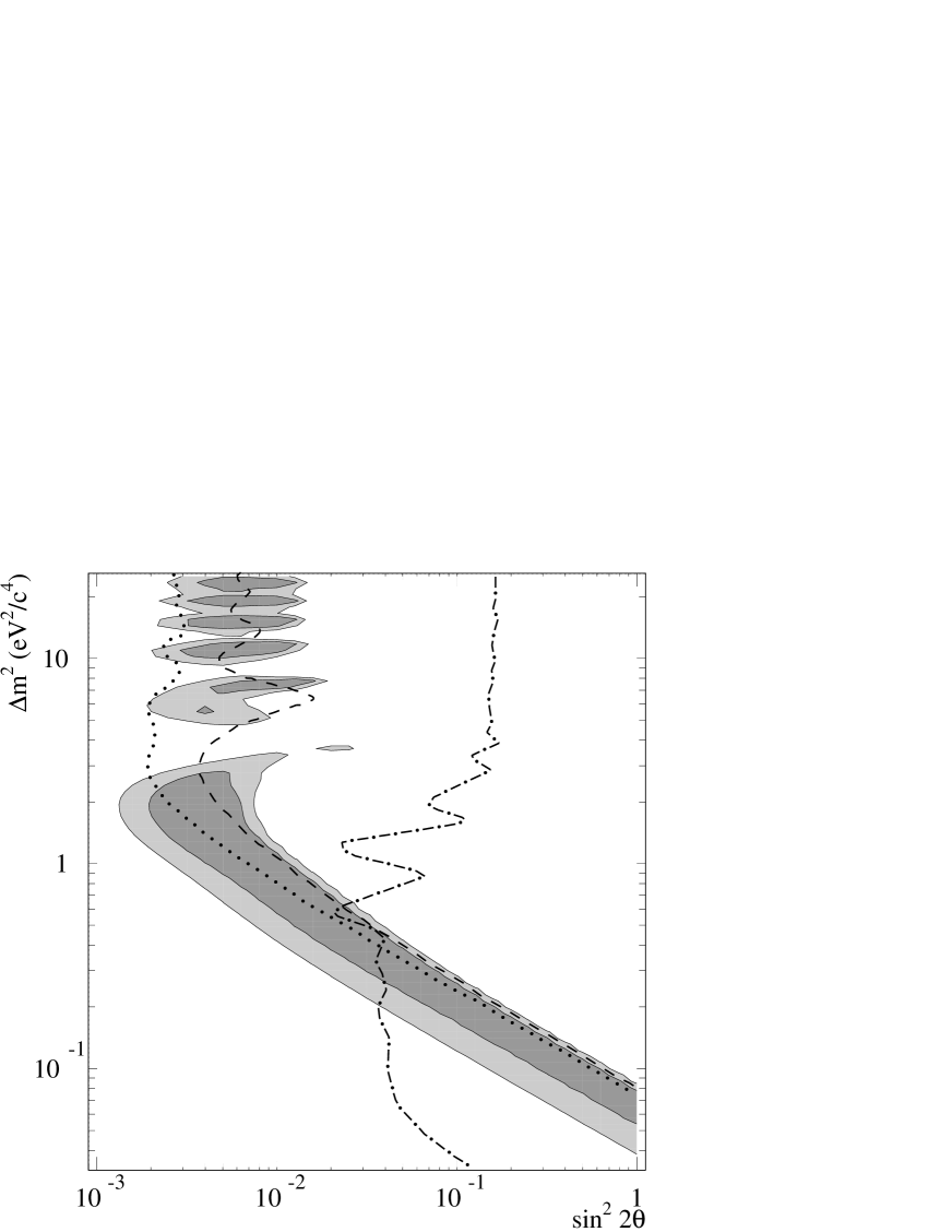
In Ref.[2] the evidence restricting neutrino oscillation parameters is briefly reviewed. The salient features of that review are repeated here. There have been a series of experiments using beams derived from pion DIF which consist dominantly of $\nu_{\mu}$ with a small $\nu_{e}$ contamination. The most sensitive experiment was at Brookhaven in a specifically designed long baseline oscillation experiment, E776 [4]. This limit is shown in Figure 1 along with the favored region obtained by the LSND experiment. The limiting systematic error in E776 is a photon background from $\pi^{\circ}$ production, where one $\gamma$ is misidentified as an electron and the second $\gamma$ is not seen. The CCFR experiment [5] provides the most stringent limit on $\nu_{\mu}\to\nu_{e}$ oscillations near $\Delta m^{2}\sim 350$ eV²/c⁴, but their limits are not as restrictive as E776 for values of $\Delta m^{2}<300$ eV²/c⁴. The KARMEN experiment [6] has searched for $\nu_{\mu}\to\nu_{e}$ oscillations using neutrinos from pion DAR. These neutrinos are monoenergetic, and the signature for oscillations is an electron energy peak at about 12 MeV. This method has very different backgrounds and systematics compared to the previous experiments but, unfortunately, does not yet have statistical precision sufficient to affect the exclusion region of Figure 1. The KARMEN experiment also has searched for $\bar{\nu}_{\mu}\to\bar{\nu}_{e}$ oscillations and has produced the exclusion plot shown in Figure 1. This is currently the most sensitive limit experiment in this channel. KARMEN is located 18 m from the neutrino source, compared with 30 m for LSND. The experiments have sensitivities, therefore, that peak at different values of $\Delta m^{2}$ .

The most sensitive experiment searching for $\bar{\nu}_{e}$ disappearance is Bugey [7] using a power reactor which is a prolific source of $\bar{\nu}_{e}$ . The detectors at Bugey observe both the positron from the primary neutrino interaction and the capture energy (4.8 MeV) from neutron absorption on $\mbox{}^{6}Li$ . The resulting limit is also shown in Figure 1.

The most sensitive searches for $\nu_{\mu}$ disappearance have been conducted by the CDHS [8] and CCFR [5] experiments. In each case two detectors are placed at different distances from the neutrino source, which is a DIF $\nu_{\mu}$ beam without focusing. The limits obtained by these experiments exclude the region with $\sin^{2}2\theta>0.08$ for values of $\Delta m^{2}$ typically above 1 eV²/c⁴ and are not as restrictive as the limits set by the appearance experiments described above. Finally, the E531 Fermilab experiment [9] searched for the appearance of tau decays from charged-current interactions in a high energy neutrino beam. This $\nu_{\mu}\to\nu_{\tau}$ oscillation search excludes the region with $\sin^{2}2\theta>0.005$ for values of $\Delta m^{2}$ above approximately 10 eV²/c⁴. Recently, the CHORUS and NOMAD experiments at CERN have reached limits close to that set by the E531 experiment with only a fraction of the data analyzed and should reach sensitivities of the order of $3\times 10^{-4}$ in $\sin^{2}2\theta$ in the near future.

C Experimental method

LSND was designed to detect neutrinos originating in a proton target and beam stop at the Los Alamos Meson Physics Facility (LAMPF), and to search specifically for both $\bar{\nu}_{\mu}\to\bar{\nu}_{e}$ and $\nu_{\mu}\to\nu_{e}$ transitions with high sensitivity. This paper focuses on the second of these two complementary searches. The neutrino source and detector are described in detail in Ref.[1], with a summary in Section II of this paper. For the DIF experimental strategy to be successful, the neutrino source must be dominated by $\nu_{\mu}$ , while producing relatively few $\nu_{e}$ by conventional means in the energy range of interest. The detector must be able to recognize $\nu_{e}$ interactions with precision and separate them from other backgrounds, many not related to the beam. The $\nu_{e}$ from conventional sources are small in number and are described in detail in Section VII.

LSND detects $\nu_{e}$ via the inclusive charged-current reaction $\nu_{e}\,C\to e^{-}\,X$ . The cross section for this process has been calculated in the continuum random phase approximation (CRPA) [10]. This calculation successfully predicts the $\nu_{e}\,C\to e^{-}\,X$ cross section from the $\mu^{+}$ DAR $\nu_{e}$ flux as measured by the LSND [11], KARMEN [12], and E225 [13] experiments. A similar calculation however predicts too large a cross section for the process $\nu_{\mu}\,C\to\mu^{-}\,X$ at higher energies. A discussion of the cross section uncertainties and comparisons to the data is presented in Section VIII. The final state electron energy can range from zero to the incident neutrino energy minus 17.3 MeV, which corresponds to the binding energy difference between the initial nucleus and the final state nucleus in the ground state.

The oscillation search analysis uses the following strategy. Beam-unrelated backgrounds induced by cosmic-ray interactions are removed as much as possible by requiring a positive identification of the electron from the $\nu_{e}\,C\to e^{-}\,X$ reaction in the tank. The remaining beam-unrelated background events in the sample are subtracted by using the data taken while the beam is off (beam-off sample) to determine the level of such background. Notice that the beam-off data is very well measured as LSND records approximately 13 times more data while the beam is off than while it is on. This procedure yields the number of excess events above cosmic background due to beam-induced neutrino processes. The remaining beam-related backgrounds are then subtracted to determine any excess above the expectation from conventional physics. The number and energy distribution of the excess events are used to determine a confidence region in the $(\sin^{2}2\theta,\Delta m^{2})$ parameter space.

This paper describes two independent analyses that use independent reconstruction techniques and different event selections. This has allowed cross checks on the software and selection criteria and has resulted in a more efficient final event selection. They shall be referred to as “analysis A” and “analysis B” throughout this paper.

D Outline of the paper

We present a brief description of the neutrino source and detector system in Section II. Section III describes the initial data selection for the DIF analysis, while the reconstruction algorithm and particle identification parameters are discussed in Section IV. Section V describes the event selection and efficiencies for two independent analyses. Distributions of the data are shown in Section VI. Section VII contains an assessment of the beam-induced neutrino backgrounds. Fits to the data and an interpretation of the data in terms of neutrino oscillations are presented in Section VIII. The conclusions are summarized in Section IX.

II Neutrino Beam, Detector and Data Collection

A The neutrino source

This experiment was carried out at LAMPF ^*^** The accelerator was operated under the name LAMPF until October 1995 when the name was changed to LANSCE (Los Alamos Neutron Scattering Center). using 800 MeV protons from the linear accelerator. Pions were produced from 14772 Coulombs of proton beam at the primary beam stop over three years of operation between 1993 and 1995. There were 1787 Coulombs in 1993, 5904 Coulombs in 1994, and 7081 Coulombs in 1995. The fraction of the total DIF neutrino flux produced in each of the three years was 12% in 1993, 42% in 1994, and 46% in 1995. The flux in 1995 was slightly reduced with respect to the Coulomb fraction due to variations in the target conditions, which are described below. The duty ratio is defined to be the ratio of data collected with beam on to that with beam off. It averaged 0.070 for the entire data sample, and was 0.072, 0.078, and 0.060 for the years 1993, 1994, and 1995, respectively.

A detailed description of the neutrino flux calculations from pion DIF in the LAMPF beam is given in Ref.[14]. A 1 mA beam of protons on the A1, A2 and A6 targets produces pions that are the source of the DIF neutrino beam [1]. The primary source of neutrinos consists of a 30-cm long water target (A6) surrounded by steel shielding and followed by a copper beam dump. It is located approximately 30 m from the center of the detector. About 3.4% of the generated $\pi^{+}$ decay in flight due to the open space between the water target and the beam stop, producing a $\nu_{\mu}$ flux with energies up to approximately 300 MeV. Most of the positive pions that decay come to rest prior to decaying. They then decay through the DAR sequence that produces the DAR neutrino fluxes via $\pi^{+}\to\mu^{+}\nu_{\mu}$ and $\mu^{+}\to e^{+}\nu_{e}\bar{\nu}_{\mu}$ , where the $\nu_{e}$ and $\bar{\nu}_{\mu}$ have a maximum energy of 52.8 MeV. Of the $\mu^{+}$ that decay, approximately 0.001% decay in flight and produce a small $\nu_{e}$ contamination of the $\nu_{\mu}$ beam. Another small contamination comes from the decay mode $\pi^{+}\to e^{+}\nu_{e}$ with a branching ratio of $1.24\times 10^{-4}$ . Together, these sources of $\nu_{e}$ constitute the major $\nu_{e}$ -induced background for the DIF analysis, as discussed in Section VII. The negative chain starting with $\pi^{-}$ leads to a smaller contamination of the beam with $\bar{\nu}_{e}$ , because the $\pi^{-}$ production cross section is suppressed by a factor of about eight relative to the $\pi^{+}$ .

The two upstream carbon targets A1 and A2 were used to generate pion and muon beams for an experimental program in nuclear physics. They are located approximately 135 m and 110 m, respectively, from the center of the detector. The flux from each target depended on the thickness as well as the proton energy in the primary beam reaching the target. They were originally 3 cm and 4 cm thick, respectively, and degraded slowly during the operation of the accelerator. Their thickness was monitored regularly during the runs and incorporated in the beam flux simulation.

The DIF neutrino flux varies approximately as $r^{-2}$ from the average neutrino production point, where $r$ is the distance traveled by the neutrino. In addition, there is a significant angular dependence of the neutrino flux with respect to the direction of the incident proton beam. Thus, the DIF neutrino flux reaching the LSND apparatus has been calculated on a three-dimensional grid that covers uniformly the entire volume of the detector. The DIF fluxes at the detector center are illustrated in Figure 2 for the positive decay chains only. Figure 2(a) shows the $\nu_{\mu}$ flux from $\pi^{+}\to\mu^{+}\nu_{\mu}$ , while Figures 2(b) and 2(c) show the most significant $\nu_{e}$ background sources from $\pi^{+}\to e^{+}\nu_{e}$ and $\mu^{+}\to e^{+}\nu_{e}\bar{\nu}_{\mu}$ , respectively. Notice that the $\nu_{\mu}$ contributions from the A1 and A2 targets are generally small compared to that from A6. However, for $\nu_{\mu}\to\nu_{e}$ oscillations with low $\Delta m^{2}$ the $\nu_{\mu}$ flux from the two upstream targets can have a significant effect.

The systematic error on the DIF flux is estimated to be 15%. The calculated flux is confirmed within 15% statistical error by the LSND measurement of the exclusive $\nu_{\mu}C\to\mu^{-}\,\mbox{}^{12}N_{gs}$ reaction [15]. This transition is very well understood theoretically, and the measurement is very clean due to the three-fold space-time correlations between the muon and the resulting decay electron and the positron emerging from the $\mbox{}^{12}N_{gs}$ $\beta$ -decay. An independent beam flux simulation, based almost entirely on GEANT 3.21 [16], has been developed in order to check the previous calculations and finds good agreement between calculated neutrino fluxes [17].

B The detector and veto shield

The detector consists of a steel tank filled with 167 metric tons of liquid scintillator and viewed by 1220 uniformly spaced $8^{\prime\prime}$ Hamamatsu photomultiplier tubes (PMT). The scintillator medium consists of mineral oil $(CH_{2})$ with a small admixture (0.031 g/l) of butyl-PBD. This mixture allows the detection of both $\check{\rm C}$ erenkov and isotropic scintillation light, so that the on-line reconstruction software provides robust particle identification (PID) for $e^{\pm}$ , along with the event vertex and electron direction. The electronics and data acquisition (DAQ) systems were designed to detect related events separated in time. This is necessary both for neutrino-induced reactions and for cosmic-ray backgrounds.

Despite 2.0 kg/cm² shielding above the detector tunnel, there remains a very large background to the oscillation search due to cosmic rays, which is suppressed by about nine orders of magnitude to reach a sensitivity limited by the neutrino source itself. The 4 kHz cosmic-ray muon rate through the tank, of which about 10% stop and decay in the scintillator, is reduced by a veto shield to a 2 Hz rate. The veto shield encloses the detector on all sides except the bottom. Additional counters were placed below the veto shield after the 1993 run to reduce cosmic-ray background entering through the bottom support structure. The main veto shield [19] consists of a 15-cm layer of liquid scintillator in an external tank, viewed by 292 uniformly spaced $5^{\prime\prime}$ EMI PMTs, and 15 cm of lead shot in an internal tank. This combination of active and passive shielding tags cosmic-ray muons that stop in the lead shot. The veto shield threshold is set to 6 PMT hits. Above this value a veto signal holds off the trigger for 15.2 $\mu$ s while inducing an 18% dead-time in the DAQ. A veto inefficiency $<10^{-5}$ is achieved off-line with this detector for incident charged particles. The veto inefficiency is larger for incident cosmic-ray neutrons.

C Detector simulation

A GEANT 3.15-based Monte Carlo is employed to simulate interactions in the LSND tank and the response of the detector system [18]. It incorporates the important underlying physical processes such as energy loss by ionization, Bremsstrahlung, Compton scattering, pair production, and $\check{\rm C}$ erenkov radiation. It also includes detector effects such as wavelength dependent light production, reflections, attenuation, pulse signal processing, and data acquisition. Much of the input to the detector response package was measured either in a test beam or in a controlled setting. Models for the transmission and absorption of light in the tank liquid were determined from measured data. The PMT characteristics, such as wavelength dependent quantum efficiencies, pulse shapes, and reflection characteristics, were measured and the results used in the simulation. The simulation is calibrated below 52.8 MeV using Michel electrons from the decay of cosmic-ray muons that stop in the detector volume. The properties of the scintillator, including absorption length and detailed characteristics of $\check{\rm C}$ erenkov radiation in this medium, are all checked in this way. The extrapolation to higher energies is then made using the MC simulation, which correctly incorporates the behavior of electrons in the detector medium.

The primary Monte Carlo data set employed to calculate selection efficiencies is called the DIF-MC data set. The neutrino flux and energy spectrum were calculated at 25 points throughout the detector volume. The DIF-MC sample is created by folding the calculated $\nu_{\mu}$ energy spectrum with the cross section predicted by the CRPA model to generate $\nu_{e}\,C\to e^{-}\,X$ interactions throughout the tank. This corresponds to 100% transmutation of the $\nu_{\mu}$ beam to $\nu_{e}$ . The events were generated inside the surface formed by the faces of the PMTs.

III Initial Data Selection

The signature for the DIF oscillation search is the presence of an isolated, high-energy electron ( $60<E_{e}<200$ MeV) in the detector from the charged-current reaction $\nu_{e}\,C\to e^{-}\,X$ . The lower energy cut at 60 MeV is chosen to be above the Michel electron energy endpoint of 52.8 MeV, while the upper energy cut at 200 MeV is the point where the beam-off background starts to increase rapidly and the signal becomes negligible. The analysis relies solely on electron PID in an energy regime for which no control sample is available. Furthermore, with the exception of the $\nu_{e}C$ reaction leading to the ${}^{12}N$ ground state, there are no additional correlations that help improve the detection of the signal.

The PID parameters used in the DAR analysis, $\chi_{a}$ , $\chi_{r}$ , $\chi_{t}$ and $\chi_{tot}$ - as defined in Ref.[2] - have been used for the DIF analysis as an initial data selection. The disadvantages in this higher energy regime are that they do not discriminate adequately against a large beam-off background and are sensitive to energy extrapolation. Thus, the initial selection uses loose cuts based on the measured distributions of $\chi_{r}$ , $\chi_{a}$ and $\chi_{tot}$ [2] just below the Michel energy endpoint ( $50<E_{e}<52$ MeV), without any energy corrections. As demonstrated by MC simulations of the DIF data (DIF-MC), this selection is effective in identifying electron events from the $\nu_{e}\,C\to e^{-}\,X$ reaction. Over the energy interval of interest ( $60<E_{e}<200$ MeV), the calculated efficiency is $98.1\pm 1.7$ %.

In order to reduce the cosmic-ray muon induced background, we require the veto shield PMT hit multiplicity be $<$ 4 for the data sample. In addition, the events were required to be reconstructed within a fiducial volume that extends up to 35 cm from the PMT faces. Space-time correlations have been used in the initial selection to reduce the background generated by the cosmic-ray muons, either directly or through the decay Michel electron. These correlations are described in the following subsections.

A Future correlations

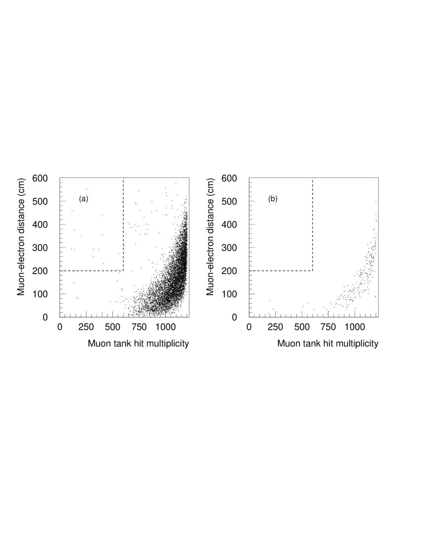
Despite the veto shield hit multiplicity requirement, some cosmic-ray muons contaminate the sample. This is seen in Figure 3, which illustrates the distribution of the time difference between the current event and all the following ones, up to 51.2 $\mu$ s. The fit to an exponential plus a constant reveals a time constant of 2.18 $\mu$ s, identifying stopped cosmic-ray muons. Cosmic-ray muons that stop and decay in the detector are uniquely identified by the following Michel electron. As illustrated in Figure 4, there is a correlation between the muon tank hit multiplicity and the distance between the reconstructed vertices of the muon-electron pair. The difference in the samples shown in Figures 4(a) and 4(b) is briefly discussed below.

Cosmic-ray muon events typically generate a high veto shield hit multiplicity. In order to suppress this high-rate background, as already mentioned in the previous section, the DAQ imposes a 15.2 $\mu$ s dead-time after each event with a veto shield hit multiplicity $\geq$ 6. Furthermore, all events with high veto shield hit multiplicities get a simpler event vertex reconstruction than the one described in Ref.[1], and no direction reconstruction. Correlations obtained from these data are shown in Figure 4(a). The number of cosmic-ray muons with veto shield hit multiplicities $<$ 6 is much lower than the ones with multiplicities $\geq$ 6, which explains the smaller size of the sample shown in Figure 4(b). Also, since these muons get both a full vertex and direction fit, the distance correlation between the muon-electron pair is tighter. In both cases, the distance correlation between the muon-electron pair degrades with increasing muon tank hit multiplicity (or equivalently, energy) due to the on-line reconstruction algorithm which always assumes a point-like event.

All events that are followed in the next 30 $\mu$ s by an event with a tank hit multiplicity between 200 and 700 (typical for Michel electrons) are possible candidates for stopped cosmic-ray muons. If, in addition, the current event has a tank hit multiplicity above 600 or is reconstructed closer than 200 cm to the following Michel electron candidate, the current event is eliminated. The events that are eliminated by this selection are almost always followed by Michel electrons, as shown in Figure 5. This selection criterion is very powerful in rejecting cosmic-ray muons and has a high efficiency for keeping candidate electron events from the $\nu_{e}\,C\to e^{-}\,X$ reaction. This efficiency is calculated to be $99.6\pm 0.4$ %.

B Past correlations

Similarly, the time difference between the current event and all of the previous activities provides a distribution indicative of Michel electrons from stopped cosmic muons in the sample, as shown in Figure 6(a). Despite the energy requirement of at least 60 MeV there is still a small contamination from the tail of the Michel electron energy spectrum. Although this problem disappears at energies above 80 MeV, we choose to impose the following selection over the entire energy regime to maintain an energy independent selection efficiency. We require that the current event have no activities in the previous 30 $\mu$ s with a tank hit multiplicity above 600 or closer than 200 cm. After imposing this cut, the time distribution with respect to previous events becomes flat, as shown in Figure 6(b). Although this cut is powerful in rejecting the high-end tails of the Michel electron spectrum, this selection has an efficiency of only $85.5\pm 0.5$ %, due to the fact that it covers the entire energy interval.

IV Event Reconstruction and Electron Identification

A Introduction

The event reconstruction and PID techniques that are used in the DIF analysis were developed to utilize fully the capabilities of the LSND apparatus. The basis for the reconstruction is a simple single track event model, parametrized by the track starting position and time $(x,y,z,t)$ , direction $(\varphi,\theta)$ , energy $(E)$ , and length $(l)$ . The coordinate system used throughout this analysis is located at the geometrical center of the detector, with the $z$ -axis along the cylindrical axis of the tank (approximately parallel to and along the beam direction) and the $y$ -axis vertical, pointing upwards. The expected PMT photon intensity and arrival time distributions for any given event are calculated from these parameters and the result is compared with the measured values. A likelihood function that relates the measured PMT charge and time values to the calculated values is used to determine the best possible event parameters and at the same time provides PID.

As mentioned in the introduction, two independent sets of reconstruction software were developed as a cross check of the analysis results. The two algorithms follow similar overall strategies but differ in detail and implementation. The main differences lie in the parametrization of the various likelihoods and probability distributions that describe the detector response, and in the set of underlying event parameters used to describe the event.

The electron identification is based on the relative likelihood of the measured PMT charges and times under the assumption that the source track is an electron. A detailed description of the physical processes in the tank can be found in Ref. [1]. Relativistic tracks in the detector generate light that falls into three categories: isotropic scintillation light that is directly proportional to the energy loss in the medium, direct $\check{\rm C}$ erenkov light emitted in a $47^{\circ}$ cone about the track direction, and isotropic scattered $\check{\rm C}$ erenkov light. These three components occur in roughly equal proportions (0.35:0.32:0.33) for relativistic particles. Only the isotropic scintillation component occurs for non-relativistic charged particles. This difference forms the basis for distinguishing electrons from non-relativistic particles such as neutrons and protons.

Each of the three light components has its own characteristic emission time distribution. The scintillation light has a small prompt peak plus a large tail which extends to hundreds of nanoseconds. The direct $\check{\rm C}$ erenkov light is prompt and is measured with a resolution of approximately 1.5 ns. The scattered $\check{\rm C}$ erenkov component has a time distribution between the direct $\check{\rm C}$ erenkov light and the scintillation light, with a prompt peak and a tail that falls off more quickly than scintillation light.

The two reconstruction algorithms used in the DIF analysis are based on maximizing the charge and time likelihood on an event-by-event basis. For any given event defined by the set of parameters $\vec{\alpha}$ ,

\vec{\alpha}=\left(x,y,z,t,\varphi,\theta,E,l\right),

(2)

the event likelihood for measuring the set of PMT charges $(q_{i})$ and times $(t_{i})$ is written as a product over the 1220 individual tank PMTs as:

{\cal L}_{event}=\prod_{i=1}^{1220}{\cal L}_{q}(q_{i};\vec{\alpha})\,{\cal L}_{t}(t_{i};\vec{\alpha}).

(3)

Reversing the meaning of the likelihood function, ${\cal L}_{event}$ is the likelihood that the event is characterized by the set $\vec{\alpha}$ , given the set of measured charges $(q_{i})$ and times $(t_{i})$ . Maximizing the event likelihood ${\cal L}_{event}$ (or equivalently minimizing $-\ln{\cal L}_{event}$ ) with respect to $\vec{\alpha}$ determines the optimal set of event parameters.

The predicted likelihoods for PMT charges and photon arrival times are based on distributions measured from a large sample of Michel electrons from stopped cosmic-ray muon decays, as described below. Analysis A uses the entire spectrum of Michel electrons, whereas analysis B uses only electrons with 38 $<$ $E_{e}$ $<$ 42 MeV, henceforth referred to as “monoenergetic”. The upper edge of the Michel spectrum (52.8 MeV) is used to calibrate the energy scale of the system. The Michel electrons are well below the critical energy of 85 MeV and result in short track segments. The extension to longer, higher energy electron tracks is made by allowing for multiple discrete sources on the track. This is done either with two sources only along the track and fitting the distance between them (i.e., the track-length) in analysis A, or with a variable number of points, as determined from the energy of the event, distributed equidistantly along the track in analysis B. The energy dependence of the event likelihood is determined from the MC simulation. In the following subsections we briefly describe the charge and time likelihoods for a pointlike source of light.

B Charge likelihood

Let us consider a pointlike light source located at $(x,y,z)$ in the detector and direction determined by $(\varphi,\theta)$ in spherical coordinates. For low energy relativistic electrons the track length is comparable with the dimensions of the PMTs, and thus the pointlike approximation provides a good model. The isotropic scintillation and scattered $\check{\rm C}$ erenkov light have a combined strength $\Phi$ (photons per steradian), where $\Phi$ is proportional to the energy $E$ of the event. The strength of the anisotropic direct $\check{\rm C}$ erenkov light is parametrized as $\rho\Phi$ , while the angular dependence is given by a nearly Gaussian function, $f(\cos\theta_{e})$ . The angle $\theta_{e}$ is the angle with respect to the reconstructed event direction of the event and the function is normalized such that

\int_{0}^{\pi}f(\cos\theta_{e})\sin\theta_{e}\,d\theta_{e}=1.

(4)

The function $f(\cos\theta_{e})$ , as determined from the data, is shown in Figure 7, with a vertical offset induced by the isotropic light.

The average number of photoelectrons (PEs) $\mu$ expected at a phototube of quantum efficiency $\varepsilon$ , at a distance $r$ from the source, and subtending a solid angle $\Omega$ is given by

\mu=\varepsilon\,\Phi\,F\left(\cos\theta_{e},r\right)\,\Omega

(5)

in analysis A. The function $F\left(\cos\theta_{e},r\right)$ is determined directly from the Michel data. In analysis B $\mu$ is parametrized as

\mu=\varepsilon\,\Phi\,\left[e^{-r/\lambda_{s}}\,\Omega_{s}+\rho\,f(\cos\theta_{e})\,e^{-r/\lambda_{c}}\,\Omega_{c}\right].

(6)

The parameters $\lambda_{s}$ and $\lambda_{c}$ are the attenuation lengths for scintillation and direct $\check{\rm C}$ erenkov light in the tank liquid, respectively. While these are indeed expected to be different for the different components of the light, the effective solid angles subtended by the PMT, $\Omega_{s}$ and $\Omega_{c}$ should, in principle, be identical. The difference is induced by the finite size of the PMTs and by the difference in the angular distributions of the two light sources [20]. Both effective solid angles have been determined from the data. Notice that although the individual quantum efficiencies of the PMTs as well as the attenuation lengths are wave-length dependent, we use only global effective values as determined from the data.

The probability of measuring $n$ PEs in the presence of the light source is then given by a Poisson distribution of mean value $\mu$ ,

P(n;\mu)=\frac{1}{n!}\,e^{-\mu}\,\mu^{n},

(7)

with $\mu$ given by Eq.(5) or Eq.(6). However, since the LSND PMTs measure charge and not the number of PEs, the probability of measuring a charge $q$ for a predicted value $\mu$ is given by

{\cal P}(q;\mu)=\sum_{n=0}^{\infty}P(q;n)P(n;\mu),

(8)

where the $P(q;n)$ functions are the charge response functions (CRFs) of the PMTs, i.e. the probability of measuring a charge $q$ given a number of PEs $n$ . Since $\mu$ depends directly on the set of event parameters $\vec{\alpha}$ , the probability ${\cal P}(q;\mu)$ determines directly the charge likelihood ${\cal L}_{q}(q;\vec{\alpha})$ for the PMT.

In analysis A the ${\cal P}(q;\mu$ ) functions are determined directly from the Michel data sample. In this sample, the predicted average number of PEs $\mu$ is calculated for every tube according to Eq.(5), for all of the events. For PMTs in a given predicted $\mu$ -bin, the distribution of the measured charge $q$ , after proper normalization, yields directly the ${\cal P}(q;\mu)$ function required for the likelihood function above. The ${\cal P}(q;\mu)$ functions obtained in this way contain all instrumental effects incurred in measuring the charge, such as saturation and threshold effects. Examples of these distributions are shown in Figure 8 for two predicted charges, $\mu$ = 0.0-0.5 PE and $\mu$ = 2.5-3.0 PE.

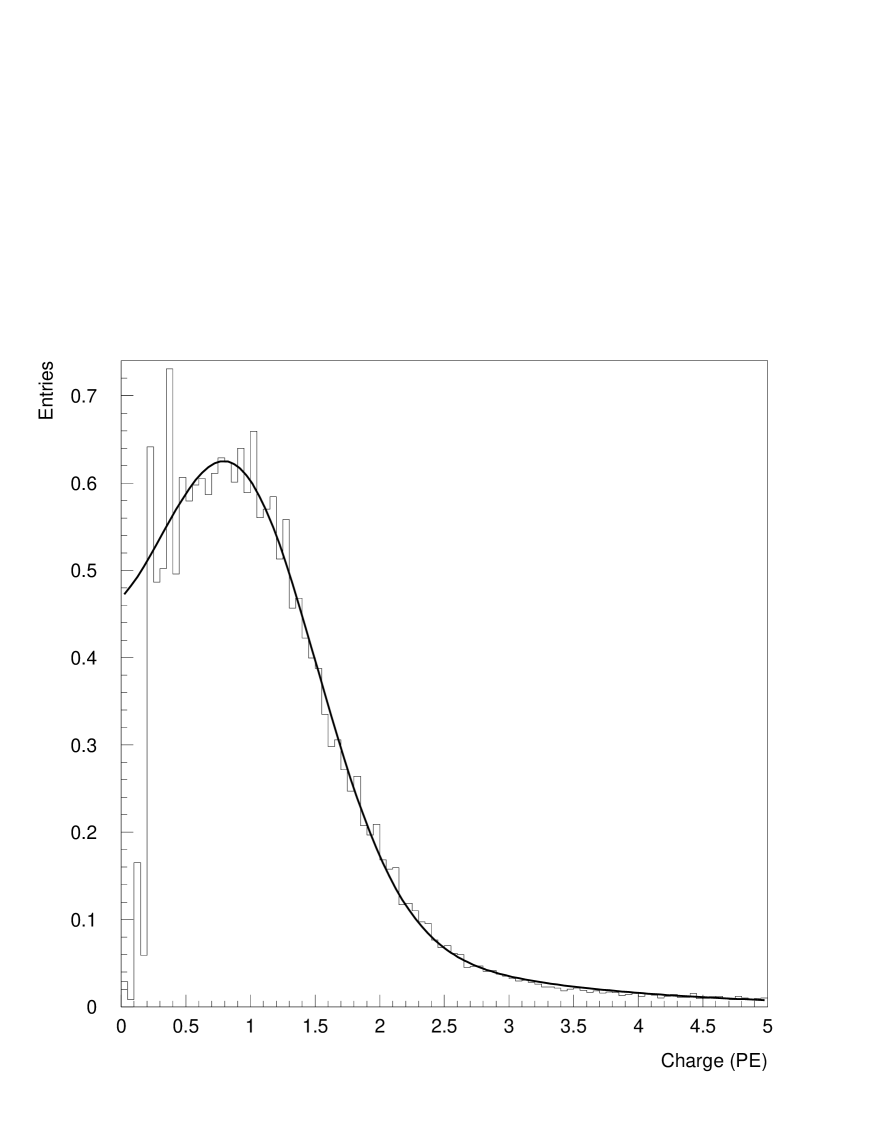
Alternatively, analysis B obtains the two lowest CRFs, $P(q;0)$ and $P(q;1)$ , and generates the higher $P(q;n)$ distributions as follows. The lowest CRF, $P(q;0)$ , is just the Kronecker delta, $\delta_{q,0}$ , since the probability of measuring a charge $q$ for no PEs vanishes identically for $q>0$ and is unity when $q=0$ . The second CRF, $P(q;1)$ , is the single-PE response of the PMTs, as illustrated in Figure 9. It is measured from low-intensity laser calibration data, taken during normal detector operation. The long tail of the single-PE charge distribution is probably due to collisions of electrons with material ahead of the first dynode. This effect is in good agreement with studies performed by the SNO experiment [21], which uses the same type of PMTs. The higher CRFs $(n\geq 2)$ are calculated by randomly sampling $P(q;1)$ $n$ times. With all CRFs normalized to unit area, the correct normalization of ${\cal P}(q;\mu)$ is automatically insured,

\int_{0}^{\infty}{\cal P}(q;\mu)\,\mbox{d}q=1,\,\,\,\,\forall\mu.

(9)

Before going on to discussing the corrected time likelihood, we should point out that both reconstructions find a slightly longer attenuation length for the direct $\check{\rm C}$ erenkov light in the MC Michel electrons than observed in the Michel electron data. This is needed to obtain agreement between the tank hit multiplicity and charge distributions obtained from the Michel electron data and the MC Michel electrons. This effect, which can be seen in Figure 7, has been shown not to affect significantly the charge and time likelihood distributions.

C Corrected time likelihood

The corrected time $t_{c}$ of a PMT is defined as the measured PMT time after corrections for the fitted event vertex time and light travel time from the event to the PMT surface. For prompt light this peaks at $t_{c}=0$ with an RMS of approximately 1.5 ns. The time response functions for scintillation light and scattered $\check{\rm C}$ erenkov light are more complicated and are determined from the Michel electron data. In addition, the time response functions depend upon the predicted charge. There is time slewing due to finite pulse rise time. There is also time jitter from the distribution of transit time of electrons in the PMT for signals with small numbers of PEs. Because the electronics responds to the first PE, above ten PEs the late tail in the distribution is negligible. Also, the amount of prompt $\check{\rm C}$ erenkov light depends on whether or not the PMT is in the $\check{\rm C}$ erenkov cone, as determined by $f(\cos\theta_{e})$ .

In analysis A the predicted average number of PEs $\mu$ is calculated for every PMT according to Eq.(5), for all events in the sample. For PMTs in a given predicted $\mu$ -bin, the distribution of the measured corrected time $t_{c}$ , after normalization to unit area, provides directly the probability $P(t_{c};\mu)$ required for the time likelihood function, ${\cal L}_{t}(t;\vec{\alpha})$ . The $P(t_{c};\mu)$ s obtained in this way contain all instrumental effects incurred in measuring the time, such as time slewing and PMT jitter. Figure 10 shows two examples of these distributions for Michel electron data and MC simulated data. Both distributions are obtained in the “isotropic” region $\cos\theta_{e}<0.3$ . Analysis A also measures the corrected time distributions in the $\check{\rm C}$ erenkov “peak” region $(0.63<\cos\theta_{e}<0.73)$ . An interpolation between these two distributions gives the time likelihood functions for the intermediate levels of direct $\check{\rm C}$ erenkov light.

The parametrization of the $P(t_{c};\mu)$ distributions of analysis B is described next. The timing distribution of the scintillation light for the LSND active medium has been measured to be of the form [22]

f(t)=A_{1}\,e^{-t/\tau_{1}}+\frac{A_{2}}{(1+t/\tau_{2})^{2}}\hskip 14.22636pt\mbox{for}\hskip 14.22636ptt\,>\,0.

(10)

The two terms above represent the fast and the slow components of the light, with time constants $\tau_{1}$ = 1.65 ns and $\tau_{2}$ = 22.58 ns, respectively. The probability for observing a corrected time $t_{c}$ is

P(t_{c})=\frac{1}{N}\int_{0}^{\infty}f(t^{\prime})\,\exp\left[-\,\frac{1}{2\sigma^{2}}\,(t_{c}-t^{\prime})^{2}\right]\,\mbox{d}t^{\prime},

(11)

which is the convolution of $f(t)$ with a time smearing function, assumed to be a Gaussian of width $\sigma$ . The overall factor $1/N$ insures proper normalization to unity. While the integration of the fast component of the light can be analytically performed, this is not true for the slow component. Therefore we choose to parametrize the scintillation light as a superposition of three exponentially decaying functions,

f(t)=\sum_{i=1}^{3}A_{i}(\mu)\,e^{-t/\tau_{i}(\mu)}.

(12)

Both the amplitudes and the time constants are also allowed to vary as a function of the predicted amount of scintillation light $\mu$ , as discussed above. The probability for recording a corrected time $t_{c}$ is thus

	$\displaystyle P(t_{c};\mu)$	$\displaystyle=$	$\displaystyle\frac{1}{N}\,\sum_{i=1}^{3}A_{i}(\mu)\int_{0}^{\infty}\exp\left[-\,\frac{1}{2\sigma^{2}(\mu)}\,(t_{c}-t^{\prime})^{2}-\frac{t^{\prime}}{\tau_{i}(\mu)}\right]\,\mbox{d}t^{\prime}$		(13)
		$\displaystyle=$	$\displaystyle\frac{1}{N}\sum_{i=1}^{3}A_{i}(\mu)\exp\left[\frac{\sigma^{2}(\mu)}{2\tau_{i}^{2}(\mu)}-\frac{t_{c}}{\tau_{i}(\mu)}\right]\mbox{Erfc}\left[\frac{1}{\sqrt{2}\sigma(\mu)}\left(\frac{\sigma^{2}(\mu)}{\tau_{i}(\mu)}-t_{c}\right)\right],$		(14)

with the normalization factor $N$ given by

N=2\,\sum_{i=1}^{3}A_{i}(\mu)\tau_{i}(\mu).

(15)

Replacing $t_{c}$ by $t_{c}-t_{0}(\mu)$ in Eq.(14) above allows for additional time slewing corrections for the scintillation light. In LSND, the time slewing calibration is performed using laser calibration data [23], which is prompt. It is expected that the scintillation light should require additional time slewing corrections, which is confirmed by the data. A typical time probability distribution as a function of the corrected time is shown in Figure 11(a). The quality of the fit to the data is excellent and shows that the parametrization given by Eq.(14) is a very good approximation.

The time distributions for the direct $\check{\rm C}$ erenkov light are also measured from the “monoenergetic” Michel electrons for different values of the predicted charge $\mu$ . This is achieved by subtracting the appropriate underlying scintillation contributions from the corrected time distributions in the $\check{\rm C}$ erenkov cone $(0.53<\cos\theta_{e}<0.79)$ . The resulting distribution is shown in Figure 11(b), which confirms the prompt character of the direct $\check{\rm C}$ erenkov light.

D Electron identification

The fitting procedures produce an accurate estimate of the amount of direct $\check{\rm C}$ erenkov light in the event. In analysis A the level of $\check{\rm C}$ erenkov light is determined after fitting the event to an electron model, i.e. a light source with an electron-like response for both charge and time likelihoods, that includes a full $\check{\rm C}$ erenkov cone. With all other event parameters fixed, the amount of direct $\check{\rm C}$ erenkov light is varied from none to the full amount for an electron event in order to maximize the event likelihood. This procedure determines a parameter $F_{Cer}$ which can thus vary between 0.0 (no direct $\check{\rm C}$ erenkov light) and 1.0 (full amount of $\check{\rm C}$ erenkov light). In analysis B the amount of $\check{\rm C}$ erenkov light is determined by varying all event parameters including $\rho$ , the $\check{\rm C}$ erenkov-to-scintillation density ratio. Figure 12 shows the distribution of the $\check{\rm C}$ erenkov-to-scintillation density ratio for “monoenergetic” Michel electrons, with a sharp peak at approximately $\rho=0.5$ . Moreover, for particles that are not expected to have any $\check{\rm C}$ erenkov light (e.g. neutrons), the algorithm finds indeed a very low $\check{\rm C}$ erenkov-to-scintillation fraction, which is still above zero because of fluctuations. This distribution is shown in Figure 13 for a sample of cosmic-ray neutrons in the same (electron-equivalent) energy range as the DIF sample. These have been tagged as neutrons by requiring the presence of a correlated $\gamma$ (from neutron capture on free protons, $np\to d\gamma$ ) with a relatively high $R_{\gamma}$ parameter, as defined in Ref.[2]. Briefly, the $R_{\gamma}$ parameter is a quantity obtained from the $\gamma$ tank hit multiplicity, time and distance distributions with respect to the primary event. As shown in Ref.[2], it provides an excellent tool for identifying correlated photons and rejecting the accidental ones.

The fitted optimum values of the charge and time negative log-likelihoods for the events are used as primary PID tools in the DIF analysis. In addition to the amount of $\check{\rm C}$ erenkov light, they prove to be very different for non-electromagnetic events (e.g. neutrons) and provide very good discrimination against them, as will be shown in the next section. Analysis A makes use of the optimal values of the overall event charge and time likelihoods, ${\cal L}_{q}$ and ${\cal L}_{t}$ , and the likelihoods calculated in the $\check{\rm C}$ erenkov cone only $(0.53<\cos\theta_{e}<0.79)$ , ${\cal L}_{qc}$ and ${\cal L}_{tc}$ . Analysis B uses instead the optimal values of the charge and time likelihoods obtained exclusively inside $(L_{Qcer},L_{Tcer})$ and outside $(L_{Qsci},L_{Tsci})$ the cone.

In both cases, the distribution of optimal likelihood values depend on the number of PMTs which were hit in a particular event. This is because the factor in the likelihood function for a PMT with a signal has a different functional form than for a tube without a signal. In order to remove this effect, the likelihoods are corrected as a function of the number of hit tubes. The mean value of the likelihood is then independent of the number of PMT hits. In addition, there is a dependence of the distribution of optimal likelihood values on the distance to the PMT wall, which is corrected for in an analogous way. Figure 14 shows the corrected distributions for analysis A as obtained from the entire Michel electron spectrum. Distributions from analysis B, as obtained from “monoenergetic” Michel electron events, are illustrated in Figure 15, before the hit multiplicity and distance corrections described above.

Both fitting algorithms significantly improve the position and direction accuracy over that used previously [2]. The spatial position resolution is now approximately 11 cm and the angle resolution is approximately $6^{\circ}$ for electron events over the energy interval of interest for this analysis. The energy resolution is limited to 6.6% at the Michel energy end-point, as stated in Ref.[1]. This is due to the width of the single-PE response of the PMTs (Figure 9) and also due to tube to tube variations in the response functions.

V Data Selection and Efficiencies

A Introduction

The event selection presented in this section is designed to reduce cosmic-ray-induced background from the initial DIF sample. At the same time, the selection criteria must efficiently identify the electron of the final state in $\nu_{e}C\to e^{-}X$ interactions. These events have the following characteristics: they have little or no activity in the veto shield system; they are nearly uniformly distributed inside the detector; they have no excess activity either before or after the event time; and they yield a track inside the tank which is consistent with an electron, as identified through the characteristic scintillation and $\check{\rm C}$ erenkov light. These are the only features available for electron event selection except in the rare case of a transition to the ${}^{12}N$ ground state, which subsequently $\beta$ -decays with a 15.9 ms lifetime.

The beam-off background data and simulated DIF-MC electron events are used in order to choose the optimal selection value for each quantity in a way unbiased by actual beam-on data. The sensitivity, or “merit” for the value of a selection parameter is defined as the efficiency $\epsilon$ (determined from the DIF-MC) divided by the square root of the number of selected beam-off events, $N_{off}$ , scaled by the duty ratio $f$ :

M\equiv\frac{\epsilon}{\sqrt{f\,N_{off}}}.

(16)

Each selection parameter value is varied and the point of maximum sensitivity, or “merit”, determines the optimal value of the selection. This method is independent of the beam-on data. Throughout this section the selection criteria for analyses A and B are discussed in parallel.

B Analyses A and B

The cosmic-ray backgrounds are dominated by several types of processes. The level of all cosmic-ray-induced processes is measured in the beam-off data sample, and then the appropriate amount is subtracted from the final beam-on sample.

Cosmic-ray neutrons generate a non-electromagnetic background. A fraction of these neutrons evade the veto shield and enter the detector volume to interact with carbon nuclei and protons in the liquid. The interaction length is approximately 75 cm. Their presence in the DIF sample is due to the very loose initial electron identification selection and can be consistently demonstrated in three different ways, as follows:

The typical signature of neutron events is the 2.2 MeV correlated $\gamma$ that results from capture on free protons, $np\to d\gamma$ . These $\gamma$ candidates are recorded in a 1000 $\mu$ s interval after the primary trigger. The time difference between the primary events of the entire DIF sample (beam on + off) and all subsequent $\gamma$ events is shown in Figure 16. The fitted lifetime of $186.2\pm 0.4$ $\mu$ s, is in very good agreement with the known neutron capture time of 186 $\mu$ s. The constant part of the fit determines the total number of accidental photons. After subtracting this number from the total number of $\gamma$ candidates in the sample one obtains that on average every DIF event has one correlated photon. This is consistent with a considerable contamination of the DIF sample by cosmic-ray neutrons, since these are expected to have on average more than one associated $\gamma$ .

Secondly, as shown in Figure 13, neutron events do not produce significant $\check{\rm C}$ erenkov light in the liquid. The distribution of the $\check{\rm C}$ erenkov-to-scintillation density ratio, $\rho$ , for the entire DIF sample (beam on + off) is shown in Figure 17 for analysis B. The same distribution for cosmic-ray neutron events with similar deposited energy and for the DIF-MC sample are superimposed. This illustrates that most of the (beam-off) background is dominated by non-electromagnetic events, consistent with neutrons. In order to select electron-like events, analysis A requires $F_{Cer}>0.7$ and analysis B requires $\rho>0.4$ , as dictated by the maximum merit algorithm. Figure 18 shows the $F_{Cer}$ and $\rho$ distributions for the DIF sample and the DIF-MC electron events after all other selection criteria have been applied.

Finally, the event charge and time likelihood parameters defined in Section IV are different for neutron and electron events. These charge and time likelihood parameters are used in differentiating electromagnetic particles that produce $\check{\rm C}$ erenkov light from non-electromagnetic backgrounds. Both analyses rely on this identification, using slightly different criteria.

Analysis A uses a likelihood ratio, $LR_{event}$ , defined by forming the product of the charge and time likelihoods in each of the regions for the DIF beam-off sample and dividing it by the same product for the DIF-MC electrons:

LR_{event}\ =\ \frac{{\cal P}(-\ln{\cal L}_{q}^{off})\times{\cal P}(-\ln{\cal L}_{qc}^{off})\times{\cal P}(-\ln{\cal L}_{t}^{off})\times{\cal P}(-\ln{\cal L}_{tc}^{off})}{{\cal P}(-\ln{\cal L}_{q}^{mc})\times{\cal P}(-\ln{\cal L}_{qc}^{mc})\times{\cal P}(-\ln{\cal L}_{t}^{mc})\times{\cal P}(-\ln{\cal L}_{tc}^{mc})}.

(17)

Figure 19 shows the individual distributions of the four ${\cal P}(-\ln{\cal L}_{x})$ functions for the beam-off data and for the DIF-MC electron data. The ratio $LR_{event}$ tends to be large for events that are like cosmic-ray background and small for electron-like events. Electron events are identified by requiring $LR_{event}$ $<$ 0.5. The event time likelihood in the $\check{\rm C}$ erenkov cone, $L_{tc}$ is also used in the selection, being sensitive to the presence of $\check{\rm C}$ erenkov light. This parameter is required to have a value $<$ 1.1. Analysis B uses only the individual time likelihoods for identifying electromagnetic particles, by requiring $L_{Tsci}<1.15$ and $L_{Tcer}<1.5$ . The charge and time negative log-likelihoods are illustrated in Figure 20 for the entire DIF data (beam on + off), DIF-MC electron events and cosmic-ray neutron events.

The second class of backgrounds is electromagnetic, and leads to events that are difficult to distinguish from pure electron events. Charged particles occasionally evade the veto shield and enter the liquid volume. These cannot travel into the liquid very far without depositing large amounts of energy and are reconstructed with a position very close to the tank wall. Their reconstructed direction points predominantly into the detector and the track can be extrapolated back to the tank wall where the veto shield information can be used. The veto counter system that surrounds the detector provides PMT signals which are read out and recorded as are the tank PMTs. For events with a non-zero veto shield hit multiplicity, $N_{veto}>0$ , the reconstructed tracks in the detector are extrapolated backwards to intersect the veto shield. A corrected time difference, $t_{veto}$ , between the veto shield hit closest in time and space and the extrapolated event time is defined. Selecting events with $|t_{veto}|>50$ ns (analysis A) or $>70$ ns (analysis B) discriminates against any cosmic-ray-induced activity around the detector near the event in question. The $t_{veto}$ distribution for the entire DIF data sample (beam on+off) is shown in Figure 21. In addition, a direct cut on the total veto hit multiplicity, $N_{veto}<3$ , is required in analysis A. Analysis B does not impose this cut. Figure 22 shows the veto shield hit multiplicity distributions for the beam-on, beam-off and beam-excess events after all selection criteria of analysis B have been applied. The distribution for the beam-excess events is consistent with the veto shield accidental hit distribution.

High energy $\gamma$ rays, from $\pi^{0}$ produced by neutron interactions in the lead shielding of the veto shield, enter the detector fiducial volume without leaving a veto signal. Energy is deposited through Compton scattering or by pair conversion. The latter process dominates above the 85 MeV critical energy of the liquid. The $\gamma$ attenuation length is roughly 50 cm, the radiation length in the liquid. The charged particles resulting from their interactions in the liquid point into the detector volume. These events are difficult to distinguish from electrons of the $\nu_{e}\,C\to e^{-}\,X$ reaction in this detector on the basis of electron identification alone.

This class of backgrounds is characterized by its typical distribution of the length of the flight-path inside the detector. This quantity is defined as the distance between the reconstructed event vertex and the intersection of the backwards extrapolation along the reconstructed event direction with the PMT surface, $\Delta$ , (analysis A) or with the tank steel wall, $S$ (analysis B). Although slightly different in their definitions, both quantities correspond to the distance a neutral particle would have to travel in the liquid before it interacts. Events were required to satisfy $\Delta>175$ cm in analysis A and $S>225$ cm in analysis B. The distributions of the $\Delta$ and $S$ variables are shown in Figure 23 for the DIF sample and the DIF-MC electron events after all other selection criteria have been applied.

Another possible source of cosmic-ray backgrounds that is reduced by the $\Delta$ and $S$ selections arises from $K_{L}^{\circ}$ decay inside the detector volume. The $K_{L}^{\circ}$ can travel into the detector where the $K_{e3}$ decay produces a positron (indistinguishable from an electron) and a $\pi^{-}$ ( $K_{L}^{\circ}\to\pi^{-}\,e^{+}\,\nu_{e}$ ). The $\pi^{-}$ will stop and be absorbed, while the positron is in the energy range of interest. The other decay chain ( $K_{L}^{\circ}\to\pi^{+}\,e^{-}\,\bar{\nu}_{e}$ ) cannot contribute to the final DIF sample due to a degraded PID generated by the muon from the pion decay being virtually simultaneous with the electron, and due to space-time correlations with the positron from the subsequent muon decay.

The electron from the $\nu_{e}\,C\to e^{-}\,X$ reaction is backward peaked, opposite the direction of the incident neutrino. Due to the geometry of the detector shielding, beam-off data favor the neutrino direction. Furthermore, the electron from one of the beam-induced backgrounds, the $\nu e\to\nu e$ elastic scattering, is also strongly peaked in the forward direction. The cosine of the angle between the reconstructed event direction and the incident neutrino direction, $\cos\theta_{\nu}$ , is used to remove most of this background, by requiring $\cos\theta_{\nu}$ $<$ 0.8 in both analyses.

The veto system is very effective at rejecting cosmic-ray-induced backgrounds, but there were several penetrations in the system. A penetration at the lower upstream end of the veto system allows cables to enter the tank. For part of the data taking period there were several poorly performing PMTs at the top of the veto system. These regions were removed from the final data set of analysis A by requiring that the projected entry points of the events not lie in the regions $(240^{\circ}<\phi_{xz}<300^{\circ},-0.2<\cos\theta_{y}<-0.6)$ and $(240^{\circ}<\phi_{xz}<300^{\circ},0.6<\cos\theta_{y}<1.0)$ . The angles $\theta_{y}$ and $\phi_{xz}$ are defined with respect to the coordinate system of the detector defined at the beginning of Section IV.

The quantities $\Delta$ , $F_{Cer}$ , $LR_{event}$ , $L_{tc}$ , $\cos\theta_{\nu}$ , $t_{veto}$ , $N_{veto}$ and the “veto hot-spots” (analysis A) and $S$ , $\rho$ , $L_{Tcer}$ , $L_{Tsci}$ , $\cos\theta_{\nu}$ and $t_{veto}$ (analysis B) are used to select a final sample of events for the DIF analysis. The values of these selection criteria, efficiencies for $\nu_{\mu}\to\nu_{e}$ events, and rejection power are shown in the Tables I and II for analyses A and B, respectively. Event selection efficiency is defined with respect to events generated inside the fiducial volume of the detector that extends all the way to the PMT surfaces ( $d>0$ cm).

Table III shows the number of beam-on, beam-off, and excess events that result from the event selections described above. There is a clear excess of events above beam-unrelated backgrounds that is consistent with $\nu_{e}\,C\to e^{-}\,X$ reactions.

Average beam-unrelated backgrounds are determined by the total number of beam-off events times the beam duty ratio. A better estimate of the beam-unrelated background in the beam-on sample relies on further information contained in the beam-off event sample. The characteristic shape of the event direction distributions in the tank coordinate system for $\nu_{e}\,C\to e^{-}\,X$ signal events are different than those for the beam-off sample. Figure 24 shows the distributions in $\cos\theta_{y}$ and $\phi_{xz}$ of the event directions for the final beam-off DIF sample as compared to the same distributions as obtained for the DIF-MC electrons.

It is possible to introduce a small bias into the event selection by using the maximum “merit” or sensitivity method to select values for the selection criteria. Because the algorithm uses the beam-off data, it can pick points where the beam-off data has fluctuated down. Even though this should be a negligible effect, the level of beam-unrelated backgrounds in the beam-on sample can also be determined nearly independently of the number in the beam-off sample. This is done by performing a maximum likelihood fit to obtain the number of beam-unrelated background events in the beam-on sample. The two-dimensional $(\cos\theta_{y},\phi_{xz})$ distribution of the beam-on event directions is fitted to a sum of the shapes expected for signal events and beam-unrelated background events. The likelihood for the total number of beam-unrelated events is weighted by the Poisson probability expected from the predicted beam-unrelated average. The results of this procedure are shown in Table IV along with the results of using the product of the duty ratio and the number of beam-off events for each analysis. The probability that the number of observed beam-on events is a fluctuation is also shown in Table IV. A systematic uncertainty of 21% in the cross section, flux, and efficiency is included in the calculation.

The comparison of selections A and B along with the logical AND and logical OR of the two samples is shown in Table V. The number of beam-on events, background events, efficiencies, and resulting oscillation probabilities are all consistent within the statistical errors in the samples. Since the two analyses have low efficiencies, different reconstruction software, and different selection criteria, the overlap need not be large. The AND sample contains 8 beam-on events, which is consistent with the 11.6 events expected by comparing the overlap of DIF-MC data and beam-off data. The final event sample is obtained as the logical OR of the events from analysis A and analysis B. This procedure minimizes the sensitivity of the measurement to uncertainties in the efficiency calculations and also yields a larger efficiency than the individual analyses. The AND sample has the lowest efficiency for DIF electron events and therefore the least sensitivity. The OR sample has the largest efficiency and hence the largest sensitivity to oscillation signals. The probability that the backgrounds in the AND and OR samples fluctuate upward to the observed beam-on numbers are 0.18 and $1.1\times 10^{-3}$ respectively.

VI Data Signal

A Distributions of data

Extensive checks have been performed on the final DIF OR sample to study the consistency with electron events from the $\nu_{e}\,C\to e^{-}\,X$ reaction. The distribution of $\cos\theta_{\nu}$ , the cosine of the angle between the reconstructed electron direction and the incident neutrino direction, is shown in Figure 25. This distribution is slightly backwards peaked, as indeed expected from the $\nu_{e}\,C\to e^{-}\,X$ reaction, and agrees well with that obtained from the DIF-MC. The distance to the PMT surfaces for the final beam-excess data set is shown in Figure 26, which also agrees with the DIF-MC expected distribution. Notice that the apparent depletion of events in the outer region of the fiducial volume is caused primarily by the $\Delta$ and $S$ selections of the two analyses. Small deviations from the original (on-line) reconstructed event vertices, induced by the new reconstruction algorithms, contribute to a smaller extent to this effect. The $x$ , $y$ and $z$ distributions for the final beam-excess DIF sample are shown in Figure 27 and are in very good agreement with those obtained from the DIF-MC simulations. The distributions of the 40 beam-on events and 175 beam-off events in the $(x,y)$ and $(y,z)$ planes are illustrated in Figure 28. The energy distribution of the beam-excess events is illustrated in Figure 29, together with the energy distribution of the beam-induced background and that expected from a positive $\nu_{\mu}\to\nu_{e}$ oscillation signal for large values of $\Delta m^{2}$ .

B Associated photons from neutron capture

The $\nu_{e}\,C\to e^{-}\,X$ reaction is not normally expected to produce free neutrons at these energies. Only rarely (approximately 10%) is a neutron knocked out by the incident neutrino, and then it is identified by the presence of a correlated 2.2 MeV $\gamma$ from the capture on free protons. Also, the small $\bar{\nu}_{e}$ contamination of the beam produces a small number of events with a correlated $\gamma$ via the inverse $\beta$ -decay reaction $\bar{\nu}_{e}\,p\to e^{+}\,n$ . The correlated $\gamma$ identification relies on the $R_{\gamma}$ parameter mentioned earlier in the text, which in turn relies on the $\gamma$ tank hit multiplicity, time and distance distributions with respect to the primary event. The reconstruction algorithms used in the current analysis provide a better position resolution not only for the primary events, but also for the $\gamma$ , as shown in Figure 30. Using the sharper distance distribution between the $\gamma$ and the primary events in the calculation of $R_{\gamma}$ provides much better discrimination between correlated and accidental $\gamma$ .

The distributions for the number of photons with $R_{\gamma}$ $>$ 1 are illustrated in Figure 31 for the final DIF beam-on, beam-off and beam-excess samples of analysis B. This particular value of the $R_{\gamma}$ cut accepts over 95% of the correlated photons, while at the same time rejecting approximately 95% of the accidental ones. The beam-induced excess yields a fraction of events with “correlated” photons $(R_{\gamma}>1)$ that is consistent with that measured in the $\nu_{\mu}\,C\to\mu^{-}\,X$ channel, as reported in [15].

C The transition to the ${}^{12}N_{gs}$

The transition $\nu_{e}\,C\to e^{-}\,{}^{12}N_{gs}$ , which is expected to occur roughly 5% of the time, is a useful signature in the search for $\nu_{\mu}\to\nu_{e}$ oscillations. It is nearly free of cosmic-ray background due to the detection of the space-time correlated positron from the ${}^{12}N_{gs}$ $\beta$ -decay [24]. It is noteworthy that the ground state of ${}^{12}N$ has been extensively studied in (p,n) reactions [25], as well as its analog, $\mbox{}^{12}C$ (15.11 MeV), in (e,e’) and (p,p’) reactions. The transition is well known and can be characterized successfully. The positron has an end-point energy of 17.3 MeV and a decay time constant of 15.9 ms. The positron selection criteria are: (i) 0.052 ms $<$ $\Delta t$ $<$ 45 ms; (ii) reconstructed distance to the primary electron $<$ 100 cm; (iii) tank hit multiplicity $>$ 75 (in order to be above the accidental $\gamma$ ray background); (iv) positron energy $<$ 18 MeV; (v) veto shield hit multiplicity $<$ 4. Using the same selection criteria for the primary electron as described above, and in addition imposing the positron space-time correlations, 2 beam-on events and 1 beam-off event are observed. However, one of the two beam-on events has three correlated $\gamma$ and is thus not consistent with the ground state hypothesis. Eliminating this event from the sample, one obtains a beam-induced excess of $0.9\pm 1.0$ events which is consistent with the expected 0.3-1.0 events, depending on the values of the oscillation parameters, as obtained from the inclusive analysis.

VII Beam-Related Backgrounds

This section discusses the beam-related backgrounds induced by neutrino interactions, which are not accounted for by the beam-off subtraction. Each of the backgrounds depends upon neutrino fluxes and cross sections that are energy dependent. The proper variation of efficiency with energy in analyses A and B is used in Sections V and VIII. In this section a generic, energy independent efficiency for electron events of 10% is assumed for the sake of clarity, a number close to the actual average values for the two analyses. The effects of systematic uncertainties on the beam-related backgrounds are crucial to the analyses. The major effects are discussed extensively in Section VIII.

There are four significant neutrino backgrounds in the $\nu_{\mu}\to\nu_{e}$ DIF oscillation search considered here. These backgrounds are: $\mu^{+}\to e^{+}\nu_{e}\bar{\nu}_{\mu}$ and $\pi^{+}\to e^{+}\nu_{e}$ DIF followed by $\nu_{e}C\to e^{-}X$ scattering; $\pi^{+}\to\mu^{+}\nu_{\mu}$ DIF followed by $\nu_{\mu}e\to\nu_{\mu}e$ elastic scattering; and $\pi^{+}\to\mu^{+}\nu_{\mu}$ DIF followed by $\nu_{\mu}C\to\nu_{\mu}C\pi^{\circ}$ coherent scattering. Backgrounds from $\nu_{\mu}C\to\mu^{-}X$ reactions are negligible. Muons that stop in the tank either decay or capture on carbon nuclei. The correlations in time and position between the muon and the secondary event removes them. In the rare case that the second event is missed, the lone muon fails the electron identification, and the event is almost always below the 60 MeV electron equivalent energy limit. In the case of $\mu^{-}$ decay in flight, the long lifetime of the muon and the electron identification requirements reduce this background to a negligible level.

The significant backgrounds are summarized in Table VI for reconstructed event energies between 60 MeV and 200 MeV. The volume used for normalization throughout this section is the $d>0$ fiducial volume, as described earlier, which contains the equivalent of $5.4\times 10^{30}$ $CH_{2}$ molecules (or $4.3\times 10^{31}$ electrons). For the combined 1993, 1994, and 1995 running periods there were $9.2\times 10^{22}$ protons on target (POT).

The largest background is due to $\nu_{e}$ that come from $\mu^{+}$ DIF in the beam stop, followed by $\nu_{e}C\to e^{-}X$ scattering in the detector. This cross section is calculated in the CRPA model [10], as already mentioned. This results in a background of 3.8 events for the assumed efficiency. The next largest is background is due to $\pi^{+}\to e^{+}\nu_{e}$ DIF in the beam stop, followed by $\nu_{e}C\to e^{-}X$ scattering in the detector. The estimated background contribution is 1.9 events. The systematic error on this contribution is discussed in Section VIII. The previous two background catagories are produced by the same reaction as the DIF oscillation signal and are nearly impossible to distinguish from them on an event-by-event basis.

Another background is coherent $\pi^{\circ}$ production via the reaction $\nu_{\mu}C\to\nu_{\mu}C\pi^{\circ}$ . This cross section has been calculated in Ref.[26]. Energetic electrons can be produced by the photons from the $\pi^{\circ}$ decay, which convert in the tank liquid and fake an electron. The fraction of $\pi^{\circ}$ that satisfy all selection criteria and are misidentified as electrons is 0.6. The estimated background contribution from coherent $\pi^{\circ}$ production is 0.3 events. Note that the non-coherent $\pi^{\circ}$ production is negligible at these energies.

The last background considered is $\nu_{\mu}e\to\nu_{\mu}e$ elastic scattering on the $4.3\times 10^{31}$ electrons in the $d>0$ fiducial volume. This purely leptonic cross section is well known theoretically. The reaction is identified by the electron direction being nearly parallel to the incident neutrino direction. The fraction of electrons within the event selection region of $\cos\theta_{\nu}<0.8$ is 0.05. The background contribution from $\nu_{\mu}e\to\nu_{\mu}e$ elastic scattering is estimated to be 0.1 events.

Table VI shows the background estimates, where the total background is calculated to be $5.8\pm 1.0$ events. The number of events expected for 100% $\nu_{\mu}\to\nu_{e}$ transmutation is 4470 events.

VIII Interpretation of the Data

This section describes the interpretation of the observed event excess in terms of the theoretically expected processes and a neutrino oscillation model. The oscillation model employed here assumes two-generation mixing, as discussed in Section I. The confidence regions in the $(\sin^{2}2\theta,\Delta m^{2})$ parameter plane are calculated in this context. The effects of systematic errors are critical to the interpretation, and are described next.

A Systematic uncertainties

The systematic uncertainties in this measurement arise from several sources. The dominant uncertainty comes from the knowledge of the underlying neutrino cross sections and the neutrino flux through the detector. The electron selection efficiency calculation also introduces some uncertainty.

The oscillation search relies on the knowledge of the $\nu_{e}\,C\to e^{-}\,X$ cross section in the 60-200 MeV electron energy range. The inclusive reaction has been calculated in the CRPA model [10] and has been measured [11]-[13] by using the $\nu_{e}$ flux from $\mu^{+}$ DAR. The DAR flux is in turn measured by the well understood ground state $\nu_{e}\,C\to e^{-}\,\mbox{}^{12}N_{gs}$ inverse $\beta$ -decay reaction. Both the ground state and the inclusive $\nu_{e}\,C$ reaction measurements agree well with the theoretical predictions, which indicates that both the flux and the cross section are predicted well. An extrapolation of the theoretical cross section must be made into the DIF energy region. We assign a systematic error of 10% to this extrapolation, based upon the agreement between the measured $\nu_{e}\,C$ data and the theoretical CRPA prediction.

The DAR $\nu_{e}$ flux endpoint is at 52.8 MeV, below the region of interest for the DIF oscillation search. The DIF neutrino flux comes from pions that decay in flight rather than from stopped $\mu^{+}$ . The $\nu_{\mu}\,C$ ground state and inclusive measurements of LSND [15] provide a check on the DIF flux. The $\nu_{\mu}\,C\to\mu^{-}\,\mbox{}^{12}N_{gs}$ ground state cross section is also well understood and is nearly independent of energy above its 123 MeV threshold. Thus, LSND measures the integral of the $\nu_{\mu}$ flux above threshold. The agreement between the predicted flux and the measured flux gives a constraint on the flux above threshold with an error of 15%. The $\nu_{\mu}\,C$ inclusive reaction cross section has a much stronger energy dependence than the ground state reaction. LSND measured this cross section [15] with high statistics and obtained a value that is approximately 45% lower than the theoretically predicted value. The calculated flux $\times$ cross section does not agree with the measured data in this case. These neutrinos are in an energy range that overlaps with the DIF $\nu_{\mu}\to\nu_{e}$ energy range and represent the same $\nu_{\mu}$ flux that the DIF oscillation search uses. It is possible that the flux $\times$ cross section for the $\nu_{e}\,C\to e^{-}\,X$ reaction also follows this trend and is lower than what we have assumed. The consequences of this are discussed below.

The next important systematic error is the extrapolation of the electron identification efficiencies to energies above the Michel endpoint of 52.8 MeV. A GEANT 3.15-based Monte Carlo calculation is used for this purpose, as described in Section II. The MC generated events were checked against Michel data taken during the 1994-1995 run periods. The electron ID efficiencies are determined in the MC Michel electron sample and in the data Michel electron sample. The differences observed in these two samples result in a 15% uncertainty in the selection efficiency. When the Michel MC sample is compared to the DIF-MC sample a lower difference of 12% is expected due to slightly narrower distributions in the DIF-MC sample.

The effect of the systematic uncertainties on the oscillation search can be explained as follows. The DIF oscillation search looks for an excess signal in the $\nu_{e}\,C\to e^{-}\,X$ process above the background from the $\nu_{e}$ contamination in the beam. This background flux is produced by the same DIF beam that produces the $\nu_{\mu}$ beam. The parent particle is dominantly either the $\mu^{+}$ or the $\pi^{+}$ . The expected average number of events is given by

\mu_{total}=\varepsilon\,\sigma_{\nu_{e}C}\,(\Phi_{\nu_{\mu}}P_{\nu_{\mu}\to\nu_{e}}+\Phi_{\nu_{e}})+\mu_{BUB}

(18)

where $\varepsilon$ is the event selection efficiency, $\Phi_{\nu_{e}/\nu_{\mu}}$ are the neutrino fluxes, $\sigma_{\nu_{e}C}$ is the neutrino cross section, and $\mu_{BUB}$ is the cosmic-ray background. The oscillation signal is proportional to the same product, $\varepsilon\,\sigma_{\nu_{e}C}\,\Phi_{\nu_{\mu}}$ , as the neutrino background, since $\Phi_{\nu_{e}}$ is proportional to $\Phi_{\nu_{\mu}}$ . The effect of lowering the product $\varepsilon\,\Phi\,\sigma_{\nu_{e}C}$ is to reduce the predicted beam-related background, i.e. the background from neutrino interactions from the $\nu_{e}$ contamination in the beam. This raises the observed oscillation signal. Only by raising the product $\varepsilon\,\Phi\,\sigma_{\nu_{e}C}$ is the oscillation signal decreased.

In order to calculate conservative confidence regions, a value of the $\varepsilon\,\Phi\,\sigma_{\nu_{e}C}$ 21% above the calculated value is assumed because of systematic uncertainties. This gives a larger confidence region because fewer of the excess events are attributed to oscillations. Then a value of $\varepsilon\,\Phi\,\sigma_{\nu_{e}C}$ 45% lower than the calculated value is assumed, consistent with the LSND $\nu_{\mu}\,C$ measurement. This has the effect of moving the lower contour to the right. The upper contour also moves somewhat to the right. The final confidence region is shown as the logical OR of the two extreme cases just described.

B Confidence regions

In order to determine the significance of the observed signal in terms of potential neutrino oscillation effects, a confidence level calculation is made in the context of a two-generation neutrino mixing model, as discussed in the Introduction. The oscillation probability is a function of the neutrino energy and the distance to the neutrino source. In the present case the distance to the source is ambiguous because of the presence of multiple beam targets, A1, A2, and A6. Therefore, the energy distribution alone is used to determine the confidence levels in the $(\sin^{2}2\theta,\Delta m^{2})$ parameter space.

The data are binned into four equal energy bins between 60 MeV and 200 MeV. In each bin the DIF-MC data are used to calculate the expected number of oscillation events, $\mu_{osc}$ , and beam-related background events, $\mu_{BRB}$ , at each $(\sin^{2}2\theta,\Delta m^{2})$ point. This number is added to the expected beam-unrelated background, $\mu_{BUB}$ , to determine the total expected number of events in each of the four energy bins:

\vec{\mu}(\sin^{2}2\theta,\Delta m^{2})=\vec{\mu}_{osc}(\sin^{2}2\theta,\Delta m^{2})+\vec{\mu}_{BRB}+\vec{\mu}_{BUB}.

(19)

From the expected numbers, a four-dimensional Poisson probability density, $p(\vec{N};\vec{\mu})$ (one dimension for each bin) of all possible results for this experiment is determined. An integration over all points in this space with a probability density greater than or equal to the measured data point value,

{\cal P}(\vec{N};\vec{\mu})\ \geq\ {\cal P}(\vec{N}_{meas};\vec{\mu}),

(20)

gives a probability for the $(sin^{2}2\theta,\Delta m^{2})$ point:

\sum_{p(\vec{N};\vec{\mu})\geq p(\vec{N}_{meas};\vec{\mu})}p(\vec{N};\vec{\mu})\,\,{\rm where}\,\vec{N}=(i,j,k,l),\,\,i,j,k,l=0,\ldots,\infty.

(21)

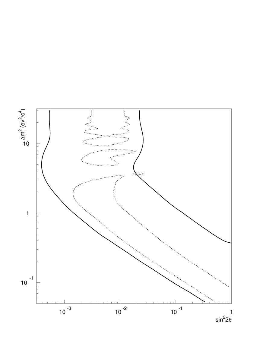
This calculation determines confidence regions, or contours of equal probability, in the $(\sin^{2}2\theta,\Delta m^{2})$ space. As discussed above in Subsection A, the calculation is made for two extreme cases of the product $\varepsilon\,\sigma_{\nu_{e}C}\,\Phi$ . The contours that result from the logical OR of these extremes are shown in Figure 32. The calculation shows that the DIF result of this paper is consistent with the previous LSND DAR result [2] in terms of the two-generation oscillation parameters.

IX Conclusions

This paper reports a search for $\nu_{e}\,C\to e^{-}\,X$ interactions for electron energies $60<E_{e}<200$ MeV. Table VI lists the expected contributions from conventional sources. This search is motivated by a high sensitivity to neutrino oscillations of the type $\nu_{\mu}\to\nu_{e}$ , due to the small contribution from conventional processes to the $\nu_{e}$ flux in this energy regime. Two independent analyses observe a number of beam-on events significantly above the expected number from the sum of conventional beam-related processes and cosmic-ray (beam-off) events. The probability that the 12.5 (14.9) estimated background events fluctuate into 23 (25) observed events is $7.0\times 10^{-3}$ ( $1.6\times 10^{-2}$ ). The excess events are consistent with $\nu_{\mu}\to\nu_{e}$ oscillations with an oscillation probability of $(2.6\pm 1.0\pm 0.5)\times 10^{-3}$ . A fit to the event distributions, assuming neutrino oscillations as the source of $\nu_{e}$ , yields the allowed region in the $(\sin^{2}2\theta,\Delta m^{2})$ parameter space shown in Figure 32. This allowed region is consistent with the allowed region from the DAR search reported earlier. This $\nu_{\mu}\to\nu_{e}$ DIF oscillation search has completely different backgrounds and systematic errors from the $\bar{\nu}_{\mu}\to\bar{\nu}_{e}$ DAR oscillation search and provides additional evidence that both effects are due to neutrino oscillations.

Acknowledgments

The authors gratefully acknowledge the support of Peter Barnes, Cyrus Hoffman, and John McClelland. This work was conducted under the auspices of the US Department of Energy, supported in part by funds provided by the University of California for the conduct of discretionary research by Los Alamos National Laboratory. This work is also supported by the National Science Foundation. We are particularly grateful for the extra effort that was made by these organizations to provide funds for running the accelerator at the end of the data taking period in 1995.

TABLE I.: Selection criteria for analysis A. For each criterion is listed: the value of the criterion; the efficiency of the criterion after all other criteria have been applied; the number of events rejected by that criterion after all other criteria have been applied; the number of beam-on, beam-off and beam-excess events prior to applying the criterion.

Criterion	Cut Value	Efficiency	$N_{rej}$	On	Off	Excess
$F_{Cer}$	$>$ 0.7	0.68	643	60	720	9.6 $\pm$ 7.7
$\Delta$	$>$ 175 cm	0.56	516	53	600	11.4 $\pm$ 7.3
$LR_{event}$	$<$ 0.5	0.89	118	32	223	16.7 $\pm$ 5.7
Veto time	$>$ 50 ns	0.98	27	26	138	16.4 $\pm$ 5.1
$cos\theta_{\nu}$	$<$ 0.8	0.95	22	24	135	14.7 $\pm$ 4.9
Hot Spots	(see text)	0.94	22	25	134	15.7 $\pm$ 4.9
$L_{tc}$	$<$ 1.1	0.98	11	23	125	14.4 $\pm$ 4.8
veto hits	$<$ 3	0.98	3	23	117	14.9 $\pm$ 4.8

TABLE II.: Selection criteria for analysis B. For each criterion is listed: the value of the criterion; the efficiency of the criterion after all other criteria have been applied; the number of events rejected by that criterion after all other criteria have been applied; the number of beam-on, beam-off and beam-excess events prior to applying the criterion.

Criterion	Cut Value	Efficiency	$N_{rej}$	On	Off	Excess
$S$	$>$ 225 cm	0.47	1009	89	1037	16.8 $\pm$ 9.7
$\rho$	$>$ 0.4	0.83	689	68	738	12.7 $\pm$ 8.5
$L_{Tsci}$	$<$ 1.15	0.90	131	34	214	19.3 $\pm$ 5.9
Veto time	$>$ 70 ns	0.96	36	27	126	18.0 $\pm$ 5.3
$cos\theta_{\nu}$	$<$ 0.8	0.95	14	27	104	19.7 $\pm$ 5.2
$L_{Tcer}$	$<$ 1.5	0.98	10	26	101	18.9 $\pm$ 4.1

TABLE III.: Event count after all selection criteria have been applied (analyses A/B).

Q_{A6}

is the number of protons on target in Coulombs.

Year	$Q_{A6}$	Beam On (A/B)	Beam Off (A/B)	Duty ratio	Excess (A/B)
1993	1787	1 / 2	17 / 21	0.072	-0.2 $\pm$ 1.0 / 0.5 $\pm$ 1.5
1994	5904	12 / 15	42 / 41	0.078	8.7 $\pm$ 3.5 / 11.8 $\pm$ 3.9
1995	7081	10 / 8	55 / 30	0.060	6.7 $\pm$ 3.2 / 6.2 $\pm$ 2.8
Total	14772	23 / 25	114 / 92	0.070	15.1 $\pm$ 4.9 / 18.5 $\pm$ 5.0

TABLE IV.: Backgrounds and observed numbers of beam-on events. The beam-unrelated cosmic backgrounds are calculated in two ways. The product of the beam duty ratio and the number of beam-off events is shown first. The correponding result for the fitted number of beam-unrelated background events in the beam-on sample is shown in parenthesis. The distinction is described in the text.

	Analysis A	Analysis B
Beam-unrelated background	8.0 $\pm$ 0.7 (6.2 $\pm$ 2.0)	6.4 $\pm$ 0.7 (5.9 $\pm$ 1.9)
Expected beam-related background	4.5 $\pm$ 0.9	8.5 $\pm$ 1.7
Total expected background	12.5 $\pm$ 1.1 (10.7 $\pm$ 2.2)	14.9 $\pm$ 1.8 (14.4 $\pm$ 2.6)
Observed beam-on events	23	25
Fluctuation probability	$7.0\times 10^{-3}$ ( $1.2\times 10^{-3}$ )	$1.6\times 10^{-2}$ ( $1.2\times 10^{-2}$ )

TABLE V.: Comparison of results for the A, B, AND, and OR data sets. The BUB is the beam-unrelated background from cosmic rays.

Sample	Beam On/Off	BUB	$\nu$ -Background	Osc. Excess	Efficiency	Osc. Probability
Analysis A	23/114	$8.0\pm 0.7$	$4.5\pm 0.9$	$10.5\pm 4.9$	0.084	$(2.9\pm 1.4)\times 10^{-3}$
Analysis B	25/ 92	$6.4\pm 0.7$	$8.5\pm 1.7$	$10.1\pm 5.3$	0.138	$(1.7\pm 0.9)\times 10^{-3}$
AND	8/ 31	$2.2\pm 0.3$	$3.1\pm 0.6$	$2.7\pm 2.9$	0.055	$(1.1\pm 1.2)\times 10^{-3}$
OR	40/175	$12.3\pm 0.9$	$9.6\pm 1.9$	$18.1\pm 6.6$	0.165	$(2.6\pm 1.0)\times 10^{-3}$

TABLE VI.: The background estimates for the

\nu_{\mu}\to\nu_{e}

oscillation search are shown for a

d>0

detector fiducial volume,

9.2\times 10^{22}

protons on target, and for reconstructed energies between 60 MeV and 200 MeV. The number of events for 100%

\nu_{\mu}\to\nu_{e}

transmutation is shown also. These numbers are illustrative for an electron selection efficiency of 0.10, independent of energy. The actual efficiencies in analyses A and B are slightly different and energy dependent.

Process	Flux (cm ${}^{-2}/$ POT)	$<\sigma>_{\nu}$ ( $10^{-40}$ cm²)	Eff.	Number of Events
$\nu_{e}C\to e^{-}X$ ( $\mu$ DIF)	$3.8\times 10^{-14}$	28.3	0.10	$3.8$
$\nu_{e}C\to e^{-}X$ ( $\pi$ DIF)	$8.3\times 10^{-15}$	79.2	0.10	$1.6$
$\nu_{\mu}C\to\nu_{\mu}C\pi^{\circ}$	$6.5\times 10^{-11}$	1.6	0.06	$0.3$
$\nu_{\mu}e\to\nu_{\mu}e$	$6.5\times 10^{-11}$	0.00136	0.005	$0.1$
Total background				$5.8$
100% $\nu_{\mu}\to\nu_{e}$ transmutation				$4470$

Refer to caption — FIG. 1.: The LSND $(\sin^{2}2\theta,\Delta m^{2})$ favored regions obtained from the $\bar{\nu}_{\mu}\to\bar{\nu}_{e}$ DAR oscillations search. The darkly-shaded and lightly-shaded regions correspond to 90% and 99% likelihood regions. Also shown are the 90% confidence level limits from KARMEN (dashed), E776 (dotted) and the Bugey reactor experiment (dot-dashed).

REFERENCES

[1] C. Athanassopoulos et. al. (LSND Collaboration), LA-UR-96-1327, to appear in Nucl. Instrum. Methods A.
[2] C. Athanassopoulos et. al. (LSND Collaboration), Phys. Rev. C 54, 2685 (1996);
C. Athanassopoulos et. al. (LSND Collaboration), Phys. Rev. Lett. 77, 3082 (1996).
[3] B. Pontecorvo, Zh. Eksp. theor. Fiz. 33, 549 (1957) [JETP 6, 429 (1958)].
[4] L. Borodovsky et. al. , Phys. Rev. Lett. 68, 274 (1992).
[5] K. S. McFarland et. al. , Phys. Rev. Lett. 75, 3993 (1995).
[6] B. Bodmann et. al. (KARMEN Collaboration), Phys. Lett. B 267 321 (1991);
B. Bodmann et. al. (KARMEN Collaboration), Phys. Lett. B 280 198 (1992);
B. Zeitnitz et. al. , Prog. Part. Nucl. Phys. 32, 351 (1994).
[7] B. Achkar et. al. , Nucl. Phys. B 434, 503 (1995).
[8] F. Dydak et. al. , Phys. Lett. B 134, 281 (1984).
[9] N. Ushida et. al. , Phys. Rev. Lett. 57, 2897 (1986).
[10] E. Kolbe, K. Langanke, and S. Krewald, Phys. Rev. C 49, 1122 (1994); (K. Langanke, private communication).
[11] C. Athanassopoulos et. al. (LSND Collaboration), Phys. Rev. C 55, 2078 (1997).
[12] B. Bodmann et. al. (KARMEN Collaboration), Phys. Lett. B 332, 251 (1994);
B. Bodmann et. al. (KARMEN Collaboration), Phys. Lett. B 339, 215 (1994).
[13] D. A. Krakauer et. al. , Phys. Rev. C 45, 2450 (1992).
[14] R. L. Burman, M. E. Potter, and E. S. Smith, Nucl. Instrum. Methods A 291, 621 (1990); R. L. Burman, A. C. Dodd, and P. Plischke, Nucl. Instrum. Methods in Phys. Research A 368, 416 (1996).
[15] C. Athanassopoulos et. al. (LSND Collaboration), LA-UR-97-1848, submitted to Phys. Rev. C.
[16] CERN Program Library Long Writeup W5013, CERN, Geneva, Switzerland.
[17] E. D. Church, P. Shriver, D. Smith, J. Waltz and D. H. White, LSND Technical Note LSND-TN-99; E. D. Church, LSND Technical Note LSND-TN-113.
[18] K. McIlhany, D. Whitehouse, A. M. Eisner, Y-X. Wang and D. Smith, “Proceedings of the Conference on Computing in High Energy Physics 1994”, LBL Report 35822, 357 (1995).
[19] J. J. Napolitano et. al. , Nucl. Instrum. Methods A 274, 152 (1989).
[20] I. Stancu, LSND Technical Note LSND-TN-106.
[21] D. Broadman, Ph.D. Thesis, Oxford University, 1992.
[22] R. A. Reeder et. al. , Nucl. Instrum. Methods A 334, 353 (1993).
[23] V. Highland, J. Margulies, I. Stancu, V. Trandafir and D. Works, in preparation, to be submitted to Nucl. Instrum. Methods A.
[24] A. Fazely, LSND Technical Note LSND-TN-108.
[25] B. D. Anderson et. al. , Phys. Rev. C 54, 237 (1996) and references therein.
[26] D. Rein and L. M. Sehgal, Nucl. Phys. B 223, 29 (1983).

Evidence for νμ→νe→subscript𝜈𝜇subscript𝜈𝑒\nu_{\mu}\to\nu_{e} Oscillations from Pion Decay in Flight Neutrinos

Abstract

pacs:

I Introduction

A Motivation

B Comparison with other experiments

C Experimental method

D Outline of the paper

II Neutrino Beam, Detector and Data Collection

A The neutrino source

B The detector and veto shield

C Detector simulation

III Initial Data Selection

A Future correlations

B Past correlations

IV Event Reconstruction and Electron Identification

A Introduction

B Charge likelihood

C Corrected time likelihood

D Electron identification

V Data Selection and Efficiencies

A Introduction

B Analyses A and B

VI Data Signal

A Distributions of data

B Associated photons from neutron capture

C The transition to the Ng​s12superscriptsubscript𝑁𝑔𝑠12{}^{12}N_{gs}

VII Beam-Related Backgrounds

VIII Interpretation of the Data

A Systematic uncertainties

B Confidence regions

IX Conclusions

Acknowledgments

REFERENCES

Evidence for $\nu_{\mu}\to\nu_{e}$ Oscillations
from Pion Decay in Flight Neutrinos

C The transition to the ${}^{12}N_{gs}$