The ¹⁴⁴Sm–$\alpha$ optical potential at astrophysically relevant energies derived from ¹⁴⁴Sm($\alpha$,$\alpha$)¹⁴⁴Sm elastic scattering

Abstract

For the determination of the ¹⁴⁴Sm–$\alpha$ optical potential we measured the angular distribution of ¹⁴⁴Sm($\alpha$,$\alpha$)¹⁴⁴Sm scattering at the energy $E_{\rm{lab}}=20~{}{\rm{MeV}}$ with high accuracy. Using the known systematics of $\alpha$–nucleus optical potentials we are able to derive the ¹⁴⁴Sm–$\alpha$ optical potential at the astrophysically relevant energy $E_{\rm{c.m.}}=9.5~{}{\rm{MeV}}$ with very limited uncertainties.

I Introduction

In a detailed study of nucleosynthesis in Type II supernovae Woosley and Howard proposed the so–called $\gamma$–process, which is important for the production of the samarium isotopes ¹⁴⁴Sm and ¹⁴⁶Sm [1]. The existence of the $\gamma$–process was confirmed later [2]. Because of the $\alpha$ decay of ¹⁴⁶Sm ($T_{1/2}=1.03\times 10^{8}~{}{\rm{y}}$) today one can find correlations between the ¹⁴²Nd/¹⁴⁴Nd ratio and the Sm/Nd ratio in some meteorites [3] as a consequence of the $\gamma$–process. The nuclear reaction rates used in the network calculations of the $\gamma$–process are relatively uncertain. Especially, the reaction rate for the production of ¹⁴⁴Sm by the photodisintegration reaction ¹⁴⁸Gd($\gamma$,$\alpha$)¹⁴⁴Sm is uncertain by a factor of 10 [4].

The reaction rate for the reaction ¹⁴⁸Gd($\gamma$,$\alpha$)¹⁴⁴Sm was derived from the ¹⁴⁴Sm($\alpha$,$\gamma$)¹⁴⁸Gd reaction cross section using a detailed–balance calculation (see e.g. [4, 5]). Usually, reaction rates are given at the relatively high temperatures of $2.5\leq T_{9}\leq 3.0$, or the capture cross section at $E_{\rm{c.m.}}=9.5~{}{\rm{MeV}}$ (corresponding to $T_{9}=2.8$) is derived [1, 4, 5, 6, 7].

Two ingredients enter into the Hauser–Feshbach calculation of the ¹⁴⁴Sm($\alpha$,$\gamma$)¹⁴⁸Gd capture cross section: transition probabilities and the nuclear level density. The transition probabilities were calculated using optical wave functions in an equivalent square well (ESW) potential [1, 4], a Woods–Saxon (WS) potential [6, 7], and a folding potential [5, 7].

Calculations with ESW potentials are very sensitive on a proper choice of the radius parameter $R$; two calculations using $R=8.01~{}{\rm{fm}}$ (Ref. [4], based on the ESW radius from Ref. [8]) and $R=8.75~{}{\rm{fm}}$ (Ref. [1], based on Ref. [9]) differ by a factor of 10 for the ¹⁴⁴Sm($\alpha$,$\gamma$)¹⁴⁸Gd cross section. The WS potential and the folding potential in Refs. [5, 6, 7] were taken from global parametrizations of $\alpha$ optical potentials; these results for the ¹⁴⁴Sm($\alpha$,$\gamma$)¹⁴⁸Gd cross section lie between the different ESW results. First experimental results on the ¹⁴⁴Sm($\alpha$,$\gamma$)¹⁴⁸Gd capture cross section at somewhat higher energies lie at the lower end of the different calculations [10].

The aim of this work is to determine the optical potential at the relevant energy $E_{\rm{c.m.}}=9.5~{}{\rm{MeV}}$. In general, optical potentials can be derived from elastic scattering angular distributions. Recently, in a systematic study the energy and mass dependence of $\alpha$–nucleus potentials was determined [11]. In that work $\alpha$ scattering on ¹⁴⁴Sm was analyzed at higher energies. An extrapolation to astrophysically relevant energies is possible only with very limited accuracy. At the energy $E_{\rm{c.m.}}=9.5~{}{\rm{MeV}}$ the ¹⁴⁴Sm($\alpha$,$\alpha$)¹⁴⁴Sm scattering cross section is given by almost pure Rutherford scattering because of the height of the Coulomb barrier of about 20 MeV. For a reliable determination of the optical potential one has to increase the energy in the scattering experiment. However, because of the energy dependence of the optical potential, the energy should be as close as possible to the astrophysically relevant energy $E_{\rm{c.m.}}=9.5~{}{\rm{MeV}}$. As a compromise we measured the ¹⁴⁴Sm($\alpha$,$\alpha$)¹⁴⁴Sm angular distribution at $E_{\rm{lab}}=20~{}{\rm{MeV}}$. At this energy the influence of the nuclear potential on the angular distribution is measurable, even though it is small. Especially the determination of the shape of the optical potential remains difficult even at this energy. For the real part this problem vanishes because its shape is given by a folding procedure, but the shape of the imaginary part has to be adjusted to the experimental angular distribution. For that reason the angular distribution has to be determined with very high accuracy in the full angular range.

The increase of the real part of the optical potential at energies close to the Coulomb barrier is well-known [12]. Close to the Coulomb barrier the number of open reaction channels changes strongly; this leads to a strong variation of the imaginary potential, and the strength of the real potential is coupled to the imaginary part by a dispersion relation. A further influence on the potential strength coming from antisymmetrization effects is indicated by microscopic calculations which were performed for light nuclei. This “threshold anomaly” (mainly so-called in heavy-ion scattering and fusion) was seen also in $\alpha$ scattering on many nuclei [11, 12, 13, 14, 15, 16].

II Experimental Setup and Data Analysis

The experiment was performed at the cyclotron laboratory at ATOMKI, Debrecen. We used the $78.8~{}{\rm{cm}}$ diameter scattering chamber which is described in detail in Ref. [17]. Here we will discuss only those properties which are important for our experiment.

A Targets and Scattering Chamber

The samarium targets were produced by the reductive evaporation method [18] at the target laboratory at ATOMKI directly before the beamtime to avoid the oxidation of the metallic samarium. A thin carbon foil (thickness $d\approx 20~{}{\rm{\mu g/cm^{2}}}$) was used as backing.

During the experiment we used one enriched ¹⁴⁴Sm and one natural Sm target, and one carbon backing without samarium layer. The enrichment in ¹⁴⁴Sm was $(96.52\pm 0.03)\%$. The thickness of the samarium targets was determined by the energy loss of the $\alpha$ particles in the samarium layer. We compared the energy of $\alpha$ particles elastically scattered on ¹²C in the carbon backing at $\vartheta_{\rm{lab}}=162^{o}$ using the pure carbon target as reference and both samarium targets. The stopping powers $dE/dx$ of the $\alpha$ particles in samarium at the relevant energies E = 20 MeV (incident $\alpha$) and E = 5.2 MeV (backward scattered $\alpha$) were taken from Ref. [19]. The resulting thicknesses are $d=142~{}{\rm{\mu g/cm^{2}}}$ (¹⁴⁴Sm) and $d=218~{}{\rm{\mu g/cm^{2}}}$ (natural Sm) with uncertainties of about 10%. The pure carbon target was used also for the angular calibration (see Sect. II C).

Additionally, two apertures were mounted on the target holder to check the beam position and the size of the beam spot directly at the position of the target. The smaller aperture had a width and height of 2 mm and 6 mm, respectively. This aperture was placed at the target position instead of the Sm target before and after each variation of the beam current. Because practically no current could be measured on this aperture the width of the beam spot was definitely smaller than 2 mm during the whole experiment, which is very important for the precise determination of the scattering angle. In contrast, the relatively poor determination of the height of the beam spot does not disturb the claimed precision of the scattering angle (see Sect. II C). Furthermore, the position of the beam on the target was continuously controlled by two monitor detectors. No evidence was found for a change of the position by determining the ratio of the count rates in both detectors (see Sect. II B).

B Detectors

For the measurement of the angular distribution we used 4 silicon surface-barrier detectors with an active area $A=50~{}{\rm{mm^{2}}}$ and thicknesses between $d=300~{}{\rm{\mu m}}$ and $d=1500~{}{\rm{\mu m}}$. The detectors were mounted on an upper and a lower turntable, which can be moved independently. On each turntable two detectors were mounted at an angular distance of $10^{o}$. Directly in front of the detectors apertures were placed with the dimensions 1.25 mm x 5.0 mm (lower detectors) and 1.0 mm x 6.0 mm (upper detectors). Together with the distance from the center of the scattering chamber $d=195.6~{}{\rm{mm}}$ (lower detectors) and $d=196.7~{}{\rm{mm}}$ (upper detectors) this results in solid angles from $\Delta\Omega=1.63\times 10^{-4}$ to $\Delta\Omega=1.55\times 10^{-4}$. The ratios of the solid angles of the different detectors were determined by overlap measurements with an accuracy much better than 1%.

Additionally, two detectors were mounted at the wall of the scattering chamber at a fixed angle of $\vartheta=15^{o}$ (left and right side relative to the beam direction). The solid angles of these detectors are $\Delta\Omega=8.10\times 10^{-6}$. These detectors were used as monitor detectors during the whole experiment.

The signals from all detectors were processed using charge-sensitive preamplifiers (PA), which were mounted directly at the scattering chamber. The output signal was further amplified by a main amplifier (MA). The bipolar output of the MA was used by a Timing Single Channel Analyzer (TSCA) to select signals with amplitudes between $\approx$ 1 V and 10 V, and the unipolar output of the MA was gated with the TSCA signal using a Linear Gate Stretcher (LGS). The LGS output was fed into an CAMAC ADC, and the ADC data were stored in a corresponding CAMAC Histogramming Memory module. The data acquisition was controlled by a standard PC with a CAMAC interface using the program MCMAIN [20]. The dead time of the system was determined by test pulses, which were fed into the test input of each PA. It turned out that the deadtime was negligible ($<0.2\%$) except the runs at very forward angles.

The achieved energy resolution was better than 0.5% corresponding $\Delta E\leq 100~{}{\rm{keV}}$ at $E_{\alpha}\approx 20~{}{\rm{MeV}}$.

C Angular Calibration

Because of the strong angular dependence of the scattering cross section especially at forward angles the angular calibration was done very carefully by two kinematic methods. The carbon backing contained some hydrogen contamination. Therefore, we used the steep kinematics of ¹H($\alpha$,$\alpha$)¹H scattering at forward angles ($10^{o}<\vartheta_{\rm{lab}}<15^{o}$). We measured the energies of the $\alpha$ particles scattered from ¹H (note: two peaks with different $\alpha$ energies corresponding to two center-of-mass scattering angles can be found at one laboratory scattering angle, labelled $\pm$ in Eq. 1) and from ¹²C (ground state and $2^{+}$ state at 4.44 MeV), and we determined the ratio

$$q^{\pm}(\vartheta)=\frac{E_{\alpha}(^{12}{\rm C}_{\rm{g.s.}})-E^{\pm}_{\alpha}(^{1}{\rm H})}{E_{\alpha}(^{12}{\rm C}_{\rm{g.s.}})-E_{\alpha}(^{12}{\rm C}_{2^{+}})}$$ (1)

from the experimentally measured energies and from a calculation of the reaction kinematics. The angular offset is given by the mean value of the differences in $\vartheta$ derived from all determined values of $q^{\pm}_{\rm{exp}}$ and $q^{\pm}_{\rm{calc}}$. The following results can be obtained from this procedure: $\Delta\vartheta_{\rm{offset}}=-0.38^{o}\pm 0.02^{o}$ (lower detectors) and $\Delta\vartheta_{\rm{offset}}=+0.32^{o}\pm 0.02^{o}$ (upper detectors). (Note that these offsets cannot be a consequence of a beam spot which is not exactly centered on the target; for the measured offset of about $0.35^{o}$ the beam spot would have been outside the aperture with a width of 2 mm, which can be placed at the position of the target, see Sect. II A.) The uncertainty of the adjustment of the angle is given by the standard deviation of each single measurement: $\Delta\vartheta_{\rm{adjust}}<\pm 0.1^{o}$ (all detectors).

In a second step we measured a kinematic coincidence between elastically scattered $\alpha$ particles and the corresponding ¹²C recoil nuclei. One detector was placed at $\vartheta_{\rm{lab},\alpha}=77^{o}$ (lower detector, left side relative to the beam axis), and the signals from elastically scattered $\alpha$ particles on ¹²C were selected by an additional TSCA. This TSCA output was used as gate for the signals from another detector which was moved around the corresponding ¹²C recoil angle $\vartheta_{\rm{lab},recoil}=42^{o}$ (upper detector, right side). The maximum recoil count rate was found almost exactly at the expected angle (see Fig. 1).

D Experimental Procedure, Uncertainties

With this setup we measured spectra from the ¹⁴⁴Sm and the natural Sm target at angles from $15^{o}$ to $172^{o}$ in steps of $1^{o}$ ($\vartheta<140^{o}$) and $2^{o}$ ($\vartheta>140^{o}$). Two typical spectra measured at forward ($\vartheta=25^{o}$) and at backward ($\vartheta=130^{o}$) angles are shown in Fig. 2. The measuring times were between some seconds (forward angles) and several hours (backward angles), and the corresponding beam currents were between 30 nA and 600 nA ⁴He²⁺ ions. The beam was stopped in a Faraday cup roughly 2 m behind the scattering chamber, and the current was measured by a current integrator.

For each run the scattering cross section was determined relative to the monitor count rate:

$$\Bigl{(}\frac{d\sigma}{d\Omega}\Bigr{)}(\vartheta)=\Bigl{(}\frac{d\sigma}{d\Omega}\Bigr{)}_{\rm{Mon}}(\vartheta=15^{o})\cdot\frac{N(\vartheta)}{N_{\rm{Mon}}(\vartheta=15^{o})}\cdot\frac{\Delta\Omega_{\rm{Mon}}}{\Delta\Omega}$$ (2)

and by assuming that the cross section at $\vartheta_{\rm{lab}}=15^{o}$ is given by pure Rutherford scattering. An absolute determination of the scattering cross section from the accumulated charge and the target thickness agrees within the quoted uncertainties with the relative determination using the monitor detectors.

In the measured angular range the cross section covers more than 4 orders of magnitude. The result of the experiment, normalized to the Rutherford cross section, is shown in Fig. 3. The error bars in Fig. 3 contain statistical uncertainties ($<1\%$ for almost any angle) and systematic uncertainties coming from the accuracy of the angular adjustment of the detectors and from contributions of other samarium isotopes in the ¹⁴⁴Sm target (chemical impurities of the targets are negligible).

At forward angles the accuracy of the angular adjustment ($<\pm 0.1^{o}$) leads to an uncertainty of about 1% in the determination of the cross section, at backward angles this uncertainty in the cross section practically disappears. In contrast, at forward angles the elastic scattering cross section of all samarium isotopes is very close to the Rutherford cross section, however at backward angles the cross section measured with the natural samarium target is about 20% to 30% smaller than the ¹⁴⁴Sm scattering cross section. Because of the high enrichment (96.52%) of the ¹⁴⁴Sm target the resulting uncertainty remains smaller than 1% even at backward angles. Therefore, we renounced of a correction of the ¹⁴⁴Sm scattering cross section.

The resulting high accuracy of this experiment is better than 2% (including both statistical and systematic uncertainties) even for the very backward angles where the cross section is more than 4 orders of magnitude smaller than at the forward angles measured in this experiment.

III Optical Model Analysis

The theoretical analysis of the scattering data was performed in the framework of the optical model (OM). The complex optical potential is given by

$$U(r)=V_{\rm C}(r)+V(r)+iW(r)$$ (3)

where $V_{\rm C}(r)$ is the Coulomb potential, and $V(r)$ resp. $W(r)$ are the real and the imaginary part of the nuclear potential, respectively.

The real part of the optical potential was calculated by a double–folding procedure:

$$V_{\rm f}(r)=\int\int\rho_{\rm P}(r_{\rm P})\,\rho_{\rm T}(r_{\rm T})\,v_{\rm eff}(E,\rho=\rho_{\rm P}+\rho_{\rm T},s=|\vec{r}+\vec{r_{\rm P}}-\vec{r_{\rm T}}|)\,d^{3}r_{\rm P}\,d^{3}r_{\rm T}$$ (4)

where $\rho_{\rm P}$, $\rho_{\rm T}$ are the densities of projectile and target, respectively, and $v_{\rm eff}$ is the effective nucleon-nucleon interaction taken in the well-established DDM3Y parametrization [21, 22]. Details about the folding procedure can be found in Refs. [16, 11], the folding integral in Eq. 4 was calculated using the code DFOLD [23]. The strength of the folding potential is adjusted by the usual strength parameter $\lambda$ with $\lambda\approx 1.2-1.3$.

The densities of the $\alpha$ particle and the ¹⁴⁴Sm nucleus were derived from the experimentally known charge density distributions [24], assuming identical proton and neutron distributions. For $N\approx Z$ nuclei up to ⁹⁰Zr ($Z=40$, $N=50$) this assumption works well, however, in the case of ²⁰⁸Pb ($Z=82$, $N=126$) a theoretically derived neutron distribution and the experimental proton distribution had to be used to obtain a good description of the elastic scattering angular distribution [11]. To take the possibility into account that the proton and neutron distributions are not identical in the nucleus ¹⁴⁴Sm ($Z=62$, $N=82$) a scaling parameter $w$ for the width of the potential was introduced, which is very close to unity. The resulting real part of the optical potential is given by:

$$V(r)=\lambda\cdot V_{\rm f}(r/w)$$ (5)

For a comparison of different potentials we use the integral parameters volume integral per interacting nucleon pair $J_{R}$ and the root-mean-square (rms) radius $r_{\rm{rms,R}}$, which are given by:

$$J_{R} = \frac{1}{A_{\rm P}A_{\rm T}}\,\int V(r)\,d^{3}r$$ (6)

$$r_{\rm{rms,R}} = \left[\frac{\int V(r)\,r^{2}\,d^{3}r}{\int V(r)\,d^{3}r}\right]^{1/2}$$ (7)

for the real part of the potential $V(r)$ and corresponding equations hold for $W(r)$. The values for the folding potential $V_{\rm f}$ at $E_{\rm{lab}}=20~{}{\rm{MeV}}$ (with $\lambda=w=1$) are $J_{R}=260.41~{}{\rm{MeVfm^{3}}}$ and $r_{\rm{rms,R}}=5.573~{}{\rm{fm}}$.

The Coulomb potential is taken in the usual form of a homogeneously charged sphere where the Coulomb radius $R_{\rm C}$ was chosen identically with the rms radius of the folding potential $V_{\rm f}$: $R_{\rm C}=r_{\rm{rms,R}}=5.573~{}{\rm{fm}}$.

For the imaginary part of the potential different parametrizations were chosen: the usual Woods–Saxon (WS) potential

$$W_{\rm{WS}}(r)=W_{0}\cdot(1+\exp{(r-R)/a})^{-p}$$ (8)

where $R$ is usually given by $R=R_{0}\cdot A_{\rm T}^{1/3}$, and a series of Fourier-Bessel (FB) functions

$$W_{\rm{FB}}(r)=\sum_{k=1}^{n}a_{k}\sin{(k\pi r/R_{\rm{FB}})}/(k\pi r/R_{\rm{FB}})$$ (9)

with the cutoff radius $R_{\rm{FB}}$.

A fitting procedure was used to minimize the deviation $\chi^{2}$ between the experimental and the calculated cross section:

$$\chi^{2}=\sum_{i=1}^{N}\Bigl{(}\frac{\sigma_{\rm{exp},i}(\vartheta)-\sigma_{\rm{calc},i}(\vartheta)}{\Delta\sigma_{\rm{exp},i}(\vartheta)}\Bigr{)}^{2}$$ (10)

The calculations were performed using the code A0 [25].

The parameters of the imaginary part, the potential strength parameter $\lambda$ and the width parameter $w$ of the real part, and the absolute value of the angular distribution were adjusted to the experimental data by the fitting procedure. The ratio $r$ of the calculated to the experimental absolute value of the angular distribution is very close to 1 in all fits: $r=1.006\pm 0.002$. Therefore, we renormalized the measured angular distribution by this ratio $r$. This renormalization of 0.6% lies well within our experimental uncertainties.

Four parametrizations of the imaginary part of the potential were used to determine the influence of the type of imaginary parametrization on the resulting volume integrals. They are labelled by 1, 2, 3 and 4 in Tabs. I and II. Labels 1 and 2 correspond to WS potentials with p=1 and p=2, respectively. For the parametrizations 3 and 4 FB-functions were used with 5 and 8 FB coefficients, respectively. The results are listed in Tabs. I and II, the calculated angular distributions are shown in Figs. 3 and 4. In addition, also the angular distribution derived from a “standard” WS potential is shown, which was used in previous calculations of the ¹⁴⁴Sm($\alpha$,$\gamma$)¹⁴⁸Gd capture cross section [6, 7]. The fits 1–4 look very similar; the $\chi^{2}/F$ varies from 1.74 to 1.82. However, the fits 3 and 4 using FB functions in the imaginary part show a slightly oscillating imaginary potential; fit 4 even shows a small unphysical region where the imaginary part becomes positive.

Of course, the $\chi^{2}/F$ of fit 5 is inferior compared to fits 1–4 because the WS parameters taken from the study of Ref. [6] were not adjusted to the experimental angular distribution.

IV Discussion

A Ambiguities of the optical potential

We extracted a definite optical potential from the experimental elastic scattering data on ¹⁴⁴Sm($\alpha$,$\alpha$)¹⁴⁴Sm at $E_{\rm{lab}}=20~{}{\rm{MeV}}$. First of all, very accurately measured scattering data are necessary for this determination, and furthermore a definite solution has to be selected from several potentials which describe the data almost identically. These problems result from discrete ambiguities (the so–called “family problem”) and from continuous ambiguities.

The problem of continuous ambiguities is reduced to a great extent by the use of folding potentials because the shape of the folding potential is better fixed compared to standard potentials of WS type. The width parameter of the folding potential, which was introduced in Sect. III should remain very close to unity; otherwise the parameters extracted from this calculation are not very reliable.

The “family problem” is illustrated in Fig. 5. Because of the reasons mentioned above we used the simplest parametrization of the imaginary potential, the standard WS type with $p=1$ as employed in fit 1. If one now varies continuously the depth of the real part of the optical potential (i. e. the strength parameter $\lambda$) and adjusts as well the width parameter $w$ and the parameters of the imaginary part to the experimental data, then one obtains a continuous variation of $w$ and $J_{R}$, but oscillations in $\chi^{2}/F$ correlated with oscillations in $J_{I}$. Each (local) minimum in $\chi^{2}/F$ – shown as data points in Fig. 5 – corresponds to one family of the optical potential. Obviously, the deepest minima in $\chi^{2}/F$ can be obtained for the families 4, 5, and 6 (see Fig. 5). This restriction on the number of the family is confirmed by the behaviour of the width parameter $w$, which should be very close to 1. Fit. 1 in Sec. III (see Figs. 3, 4) can be found here as family 4.

A more detailed analysis of the resulting real potentials shows that all potentials have the same depth at the radius $r=10.61~{}{\rm{fm}}$: $V(r=10.61~{}{\rm{fm}})=-0.54~{}{\rm{MeV}}$. This result is shown in Fig. 6. (An exception was found for family 1, but for the region of this family $\chi^{2}/F$ does not show a certain minimum, see Fig. 5.) A similar result was already found by Badawy et al. [26] by analyzing excitation functions of $\alpha$ scattering measured close to $\vartheta=180^{o}$ at energies $10~{}{\rm{MeV}}\leq E_{\rm{lab}}\leq 20~{}{\rm{MeV}}$: These authors stated that “at energies near the Coulomb barrier the $\alpha$–particle scattering data are fitted by any Woods–Saxon potential whose depth at $r=R_{0}$ is 0.2 MeV”. For ¹⁴⁴Sm they derived $R_{0}=11.04\pm 0.02~{}{\rm{fm}}$. However, in contradiction to that statement we point out that one has to choose one of the discrete values of the real volume integrals $J_{R}$ determined by the minima in $\chi^{2}/F$ (families 1–11). Choosing e.g. a strength parameter $\lambda=1.35$ (which is exactly between families 4 and 5) and adjusting $w$ so that $V(r=10.61~{}{\rm{fm}})=-0.54~{}{\rm{MeV}}$ ($w=1.018$) results in a significantly worse description of the experimental data ($\chi^{2}/F=1.92$ compared to $\chi^{2}/F=1.82$ for families 4 and 5). Of course, this discrimination is only possible if very accurately measured scattering data are available!

The “family problem” usually can be solved at higher energies. The ¹⁴⁴Sm($\alpha$,$\alpha$)¹⁴⁴Sm scattering data at $E_{\rm{lab}}=120~{}{\rm{MeV}}$ [27] can be described well by a calculation using a folding potential with $J_{R}=286.8~{}{\rm{MeVfm^{3}}}$ [11], and a similar volume integral was found in Ref. [27] using WS potentials. Together with the systematic behaviour of folding potentials for nuclei with $A\geq 90$ [11] which can be described by the interplay of the energy dependence of the NN interaction $v_{\rm eff}$ and the effect of the so–called “threshold anomaly” [12, 16] one expects volume integrals of about $J_{R}\approx 330-340~{}{\rm{MeVfm^{3}}}$ at the low energies analyzed in this work (see Fig. 7, upper part and Sect. IV B). ¿From this point of view we can decide that family 4 corresponds to the volume integral $J_{R}(E_{\rm{lab}}=120~{}{\rm{MeV}})=286.8~{}{\rm{MeVfm^{3}}}$.

There is a further confirmation for family 4. The ground state wave function of ¹⁴⁸Gd_g.s. = ¹⁴⁴Sm $\otimes$ $\alpha$ can be calculated [11]. The number of nodes $N$ and the angular momentum $L$ of the $\alpha$ particle outside the ¹⁴⁴Sm core are related to the oscillator quantum number $Q$ by

$$Q=2N+L=\sum_{i=1}^{4}(2n_{i}+l_{i})=\sum_{i=1}^{4}q_{i}.$$ (11)

Using $Q=18$ (corresponding to $q_{i}=5$ oscillator quanta for each neutron in the $2f_{7/2}$ shell and $q_{i}=4$ oscillator quanta for each proton in the $2d_{5/2}$ shell, see e.g. [28]) one has to adjust the folding potential strength to reproduce the binding energy of the ¹⁴⁸Gd ground state. One obtains $\lambda=1.159$ and $J_{R}=311.2~{}{\rm{MeVfm^{3}}}$ at E = +3.2 MeV (the nucleus ¹⁴⁸Gd decays by $\alpha$ emission) which fits into the known systematic behaviour of $\alpha$-nucleus volume integrals [11].

For all these reasons we chose the calculations corresponding to family 4 with $J_{R}\approx 349~{}{\rm{MeVfm^{3}}}$ and $J_{I}\approx 52.5~{}{\rm{MeVfm^{3}}}$ (see Sect. III) obtained with the standard WS parametrization of the imaginary part (fit 1 in Tabs. I and II).

B Extrapolation to $E_{\rm{c.m.}}=9.5~{}{\rm{MeV}}$

For the calculation of the ¹⁴⁴Sm($\alpha$,$\gamma$)¹⁴⁸Gd reaction cross section at the astrophysically relevant energy $E_{\rm{c.m.}}=9.5~{}{\rm{MeV}}$ one has to determine the optical potential at that energy. The following methods were applied to extract the real and imaginary part of the potential.

In a first step the folding potential in the real part was calculated at the energy $E_{\rm{c.m.}}=9.5~{}{\rm{MeV}}$ (this is necessary because of the energy dependence of the interaction $v_{\rm eff}$, see Eq. 4). Second, the width parameter $w$ was taken from fit 1: $w=1.022$. Third, because of the rise of the volume integrals $J_{R}$ at low energies which is about $\Delta J_{R}/\Delta E\approx 1-2~{}{\rm{MeVfm^{3}/MeV}}$ [11] we adjusted the parameter $\lambda$ to obtain a volume integral of $J_{R}(E_{\rm{c.m.}}=9.5~{}{\rm{MeV}})=334\pm 6~{}{\rm{MeVfm^{3}}}$: $\lambda=1.1965\pm 0.0216$. The uncertainties of $J_{R}$ and $\lambda$ were estimated from the uncertainties of $\Delta J_{R}/\Delta E$ and $J_{R}(E_{\rm{lab}}=20~{}{\rm{MeV}})$.

The volume integral of the imaginary part can be parametrized according to Brown and Rho (BR) [29]:

$$J_{I}(E_{\rm{c.m.}})=\left\{\begin{array}[]{rll}&\lx@intercol\hfil 0\hfil\lx@intercol&{\mbox{for~{}}}E_{\rm{c.m.}}\leq E_{0}\\ &J_{0}\cdot\frac{(E_{\rm{c.m.}}-E_{0})^{2}}{(E_{\rm{c.m.}}-E_{0})^{2}+\Delta^{2}}&{\mbox{for~{}}}E_{\rm{c.m.}}>E_{0}\\ \end{array}\right.$$ (12)

with the excitation energy $E_{0}$ of the first excited state, and the saturation parameter $J_{0}$ and the rise parameter $\Delta$, which are adjusted to the experimentally derived values.

¿From the ¹⁴⁴Sm scattering data at $E_{\rm{lab}}=20~{}{\rm{MeV}}$ and $E_{\rm{lab}}=120~{}{\rm{MeV}}$ [27] one obtains $J_{0}=79.98~{}{\rm{MeVfm^{3}}}$ and $\Delta=12.84~{}{\rm{MeV}}$. The excitation energy of the first excited $2^{+}$ state in ¹⁴⁴Sm is $E_{0}=1.660~{}{\rm{MeV}}$. This leads to a volume integral at $E_{\rm{c.m.}}=9.5~{}{\rm{MeV}}$ of $J_{I}(E_{\rm{c.m.}}=9.5~{}{\rm{MeV}})=21.7~{}{\rm{MeVfm^{3}}}$. Because of the weak mass dependence of the imaginary part for heavy nuclei with a magic neutron or proton number (see Fig. 7, lower part) and because the BR parametrization is not very well defined by 2 data points (and 2 parameters to be adjusted!) we also used the well–defined BR parametrization for ⁹⁰Zr taken from Ref. [11]: $J_{0}=84.3~{}{\rm{MeVfm^{3}}}$ and $\Delta=11.8~{}{\rm{MeV}}$. This leads to $J_{I}(E_{\rm{c.m.}}=9.5~{}{\rm{MeV}})=25.5\pm 0.3~{}{\rm{MeVfm^{3}}}$ using either $E_{0}=1.66~{}{\rm{MeV}}$ adjusted to ¹⁴⁴Sm or $E_{0}=1.78~{}{\rm{MeV}}$ adjusted to ⁹⁰Zr. Combining the values derived from the BR parametrizations of ¹⁴⁴Sm and ⁹⁰Zr, we adopt a volume integral of $J_{I}(E_{\rm{c.m.}}=9.5~{}{\rm{MeV}})=22.5^{+3.0}_{-1.5}~{}{\rm{MeVfm^{3}}}$.

The shape of the imaginary potential is not as certain as its volume integral. Several parametrizations lead to almost identical fits at $E_{\rm{lab}}=20~{}{\rm{MeV}}$. For our extrapolation we used the geometry of the potential derived in fit 1 (see Tabs. I and II), because the shape of the imaginary potential should not change dramatically from $E_{\rm{lab}}=20~{}{\rm{MeV}}$ to $E_{\rm{c.m.}}=9.5~{}{\rm{MeV}}$, and we adjusted the depth $W_{0}=4.55^{+0.61}_{-0.30}~{}{\rm{MeV}}$ to obtain a potential with the correct imaginary volume integral.

C ¹⁴⁴Sm($\alpha$,$\gamma$)¹⁴⁸Gd and the ¹⁴⁶Sm/¹⁴⁴Sm production ratio

Reaction rates for the reaction ¹⁴⁴Sm($\alpha$,$\gamma$)¹⁴⁸Gd at $T_{9}=2.5$ and $T_{9}=3.0$ are listed in Tab. III. To determine the influence of the optical potential on the ¹⁴⁴Sm($\alpha$,$\gamma$)¹⁴⁸Gd cross section the calculations of Refs. [5, 7] were repeated only changing the optical potentials. Compared to a previous calculation using a folding potential with parameters derived from a global systematics [5, 7] the reaction rate is reduced by a factor of about 1.5. The optical potential is well–defined by the scattering data. With the optical potential determined in this work the calculated and the preliminary experimental ¹⁴⁴Sm($\alpha$,$\gamma$)¹⁴⁸Gd capture cross section agree reasonably well.

The reaction rate does not depend strongly on the chosen family because the scattering data are reproduced quite well from calculations using potentials of families 3, 4, and 5. The capture cross section decreases (increases) by about 11% (10%) using family 3 (5) instead of family 4. A similar increase of about 8% compared to family 4 is obtained when one uses a potential between families 4 and 5 as mentioned in Sect. IV A because of the somewhat larger imaginary part of the potential.

The influence of the reaction rate on the ¹⁴⁶Sm/¹⁴⁴Sm production ratio was analyzed in Ref. [4]. Our reduced reaction rate lies between cases C and D of Tab. I in Ref. [4] corresponding to a production ratio of about 0.3 which is well between the experimentally derived limits of 0.1 to 0.7 [3].

V Conclusion

The elastic scattering cross section ¹⁴⁴Sm($\alpha$,$\alpha$)¹⁴⁴Sm was measured at $E_{\rm{lab}}=20~{}{\rm{MeV}}$ with very high accuracy. A definite optical potential could be derived from the experimental data and by taking into account the systematics of $\alpha$–nucleus optical potentials of Ref. [11]. Again using this systematics, an extrapolation of the optical potential from $E_{\rm{lab}}=20~{}{\rm{MeV}}$ to the astrophysically relevant energy $E_{\rm{c.m.}}=9.5~{}{\rm{MeV}}$ was possible with very limited uncertainties. The ¹⁴⁴Sm($\alpha$,$\gamma$)¹⁴⁸Gd cross section is reduced by a factor of about 1.5 compared to a previous folding potential calculation, it still lies between the two ESW calculations differing by a factor of 10. The uncertainty of the ¹⁴⁴Sm($\alpha$,$\gamma$)¹⁴⁸Gd cross section coming from continuous and discrete ambiguities of the optical potential is reduced by a great amount. The use of systematic folding potentials is highly recommended for the analysis of low–energy $\alpha$ scattering and $\alpha$ capture reactions because of the reduced number of free parameters compared to previous calculations using WS potentials, resp. because of the reduced uncertainties in the radius parameter compared to ESW calculations.

TABLE I.: Potential parameters of the imaginary part of the optical potential derived from the angular distribution of ¹⁴⁴Sm($\alpha$,$\alpha$)¹⁴⁴Sm at $E_{\rm{lab}}=20~{}{\rm{MeV}}$.

fit	$W_{0}~{}({\rm{MeV}})$	$R_{0}~{}({\rm{fm}})$	$a~{}({\rm{fm}})$	$p$
1	10.64	1.6758	0.1680	1
2	10.70	1.7132	0.2265	2
fit	$R_{\rm{FB}}~{}({\rm{fm}})$	$a_{1}$	$a_{2}$	$a_{3}$	$a_{4}$	$a_{5}$	$a_{6}$	$a_{7}$	$a_{8}$
3	15.0	-11.65	-16.66	6.09	21.31	10.79	-	-	-
4	15.0	-9.50	-6.50	19.42	14.84	-23.51	-35.83	-14.88	-1.06
5 a	$V_{0}=185~{}{\rm{MeV}}$, $W_{0}=25~{}{\rm{MeV}}$, $R_{0,R}=R_{0,I}=1.4~{}{\rm{fm}}$, $a_{R}=a_{I}=0.52~{}{\rm{fm}}$

TABLE II.: Integral potential parameters $J$ and $r_{\rm{rms}}$ of the real and imaginary part of the optical potential derived from the angular distribution of ¹⁴⁴Sm($\alpha$,$\alpha$)¹⁴⁴Sm at $E_{\rm{lab}}=20~{}{\rm{MeV}}$.

fit	$\lambda$	$w$	$J_{R}$	$r_{\rm{rms,R}}$	$J_{I}$	$r_{\rm{rms,I}}$	$\chi^{2}/F$
No.			$({\rm{MeVfm^{3}}})$	$({\rm{fm}})$	$({\rm{MeVfm^{3}}})$	$({\rm{fm}})$
1	1.2568	1.0220	349.34	5.6961	52.57	6.8311	1.823
2	1.2580	1.0216	349.29	5.6940	52.41	6.8142	1.823
3	1.3425	0.9976	347.04	5.5600	57.49	6.0756	1.807
4	1.2771	1.0067	339.31	5.6110	51.30	6.8868	1.738
5 a	Woods–Saxon		557.59	6.0026	75.35	6.0026	41.0

TABLE III.: Reaction rates of ¹⁴⁴Sm($\alpha$,$\gamma$)¹⁴⁸Gd at temperatures of $T_{9}=2.5$ and $T_{9}=3.0$.

potential	potential	($\alpha$,$\gamma$)	$N_{A}\cdot<\sigma v>~{}({\rm{cm^{3}\,s^{-1}\,mole^{-1}}})$
	from Ref.	from Ref.	$T_{9}=2.5$	$T_{9}=3.0$
ESW, R = 8.01 fm	[8]	[4]	3.72 $\times$ 10-16	2.58 $\times$ 10-13
ESW, R = 8.75 fm	[9]	[1]	3.75 $\times$ 10-15	2.35 $\times$ 10-12
WS	[6]	[6, 7]	1.95 $\times$ 10-15	1.22 $\times$ 10-12
Folding, $\lambda=1.159$	[5, 7]	[5, 7]	1.27 $\times$ 10-15	7.56 $\times$ 10-13
Folding	this work	this work	7.91 $\times$ 10-16	5.63 $\times$ 10-13

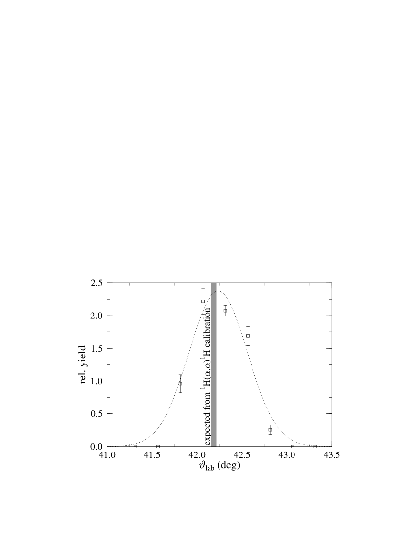
FIG. 1.: Relative yield of ¹²C recoil nuclei in coincidence with elastically scattered $\alpha$ particles. The shaded area shows the angle and the uncertainty which is expected from the calibration using the steep kinematics of ¹H($\alpha$,$\alpha$)¹H. The dotted line is a Gaussian fit to the experimental data points to guide the eye.

FIG. 2.: Typical spectra of ¹⁴⁴Sm($\alpha$,$\alpha$)¹⁴⁴Sm at $\vartheta_{\rm{lab}}=25^{o}$ (upper diagram) and at $\vartheta_{\rm{lab}}=130^{o}$ (lower diagram).

FIG. 3.: Elastic scattering cross section of ¹⁴⁴Sm($\alpha$,$\alpha$)¹⁴⁴Sm normalized to the Rutherford cross section. The line is the result of an OM calculation using folding potentials and corresponds to fit 1 of Tabs. 1 and 2 (see Sect. III). The inserts show magnifications of the forward and backward angular range.

FIG. 4.: Calculated elastic scattering cross section of ¹⁴⁴Sm($\alpha$,$\alpha$)¹⁴⁴Sm normalized to the Rutherford cross section. The lines are the result of different OM calculations using folding potentials (fits 1–4, which have almost the same $\chi^{2}/F$) and using a standard WS potential (fit 5) from Ref. [6]. The parameters are shown in Tabs. 1 and 2.

FIG. 5.: Parameters of different families (numbered 1–11) of optical potentials derived from the ¹⁴⁴Sm($\alpha$,$\alpha$)¹⁴⁴Sm scattering data: strength parameter $\lambda$, width parameter $w$, volume integrals of the real and imaginary part $J_{R}$ resp. $J_{I}$, and the deviation per degree of freedom $\chi^{2}/F$ (from top to bottom). The data points are results of fits of real and imaginary part using different starting values, the lines are the result of an interpolation in $\lambda$ and $w$ to adjust the real part of the potential to $V(r=10.61~{}{\rm{fm}})=-0.54~{}{\rm{MeV}}$, and the imaginary part of the potential was again adjusted to the experimental data. The deepest minima in $\chi^{2}/F$ are obtained for the families 4, 5, and 6.

FIG. 6.: Real part of different families of optical potentials (labelled 1–11) derived from the ¹⁴⁴Sm($\alpha$,$\alpha$)¹⁴⁴Sm scattering data: in the insert one can see that all potentials have the same depth at the radius $r=10.61~{}{\rm{fm}}$: $V(r=10.61~{}{\rm{fm}})=-0.54~{}{\rm{MeV}}$. For family 1 (dashed line) one finds an exception but for the region of this family $\chi^{2}/F$ does not show a certain minimum (see Fig. 5).

FIG. 7.: Volume integrals of the real (upper) and imaginary part (lower diagram) of the optical potential derived from ¹⁴⁴Sm($\alpha$,$\alpha$)¹⁴⁴Sm scattering. For comparison the volume integrals derived from ⁹⁰Zr($\alpha$,$\alpha$)⁹⁰Zr scattering [11] were added. The lines in the lower diagram show the results of BR parametrizations of the imaginary part (see text).