OBSERVATION OF A UNITARY CUSP IN THE THRESHOLD ${\gamma}p\rightarrow\pi^{0}p$ REACTION

Abstract

A rigorous multipole analysis of the recent ${\gamma}p\rightarrow\pi^{0}p$ cross section measurement is presented. The data were taken using the photon spectrometer TAPS at the tagged photon beam of the Mainz microtron. The s and p wave multipoles were extracted using minimal model assumptions. The predicted unitary cusp for the s wave multipole $E_{0+}$ due to the two step ${\gamma}p\rightarrow\pi^{+}n\rightarrow\pi^{0}p$ reaction was observed. The results are consistent with one loop chiral perturbation theory calculations for which three low energy constants have been determined by a fit to the data. The uncertainties in the analysis and the need for polarization observables are discussed.

1 Introduction

Experiments on photo-pion production from the nucleon are important because the pion is approximately a Goldstone Boson of QCD [1]. The consequences of this are a relatively small mass (due to the small up and down quark mass) and a weak ${\pi}N$ interaction at low energies [1]. These characteristics allow a QCD based approximation scheme known as chiral perturbation theory (ChPT) [1, 2, 3]. Using this technique extensive (1 loop) calculations for threshold photo- and electro-pion production have been performed [4].

For a long time there has been a predicted unitary cusp in the s wave ${\gamma}p\rightarrow\pi^{0}p$ electric dipole amplitude, $E_{0+}({\gamma}p\rightarrow\pi^{0}p)$, due to the two step ${\gamma}p\rightarrow\pi^{+}n\rightarrow\pi^{0}p$ reaction [5]. The reason is that the electric dipole amplitude for the ${\gamma}p\rightarrow\pi^{+}n$ reaction, $E_{0+}({\gamma}p\rightarrow\pi^{+}n)$, is more than an order of magnitude larger then $E_{0+}({\gamma}p\rightarrow\pi^{0}p)$ and also because the threshold energies for the ${\gamma}p\rightarrow\pi^{0}p$ and $\pi^{+}n$ channels are different (see Table 1). For this reason the unitary cusp is isospin violating.

The magnitude of the cusp is related to

$$\beta=E_{0+}({\gamma}p\rightarrow\pi^{+}n)\cdot a_{cex}(\pi^{+}n\leftrightarrow\pi^{0}p)$$ (1)

where $a_{cex}$ is the s wave charge exchange scattering length. Recently it was pointed out that an accurate measurement of the energy dependence of the unitary cusp would allow one to make a measurement of this important and previously unmeasured scattering length [6]. Furthermore it was also shown that the two step reaction is expected to exhibit an additional isospin violation [6] as a consequence of the predicted isospin violation in $a_{cex}$ due to the mass difference of the up and down quarks [7]. Consequently, experimental tests of the predictions of ChPT [4] and the unitary cusp with its light quark dynamics are of great importance.

The first measurement of the ${\gamma}p\rightarrow\pi^{0}p$ threshold cross sections with a 100% duty cycle electron accelerator was performed at Mainz [8]. The data confirmed a previously measured total cross section at Saclay [9] which was obtained with a 1% duty cycle linac and consequently had larger errors. The Mainz differential cross section qualitatively showed the predicted unitary cusp for $E_{0+}$ [10]. The original interpretation of the differential cross section data [8, 9] showed a disagreement with the “Low Energy Theorems” (LET) [11, 12]. However it was later shown [13] that when the total cross section data were included that the results were consistent with the LET prediction [11]. Subsequently it was shown that the LET were slowly converging [4, 12] and that the prediction for $E_{0+}$ should be significantly smaller in magnitude. The exact value is not predicted by ChPT since it depends on low energy constants which have to be evaluated from experiment [4]. It was clear that such an important measurement should be repeated with improved equipment. A subsequent experiment was performed at Mainz with the TAPS photon detector [15] where the data from threshold to 152 MeV were presented after a preliminary analysis.

In this paper a more thorough analysis from threshold to 160 MeV will be presented. The main purpose of this paper is to obtain the most accurate values of the multipoles with the minimum number of model dependent assumptions and to compare these results with the ChPT fit [4]. A secondary purpose is to show the model dependence of the extracted multipoles and the limits due to the fact that the existing database contains only unpolarized cross sections. The results presented here are in good agreement, as expected, with our previous publication [15]. Recently an experiment from Saskatoon has been reported [16] and will also be discussed.

2 Formulas and Data Analysis

Near threshold one can safely assume that the pions are produced in s and p wave states. The differential and total cross sections are:

$$\begin{array}[]{c}\sigma(\theta)=q/k[A+Bcos(\theta)+Ccos^{2}(\theta)]\\ \sigma_{T}=4\pi q/k[A+C/3]\end{array}$$ (2)

where $q$ and $k$ are the pion and photon center of mass momenta.

It is conventional to compare theory and experiment in terms of multipole amplitudes. These are: s wave electric dipole $E_{0+}$; p wave magnetic dipole with $j=1/2$ $M_{1-}$; and p wave magnetic dipole and electric quadrupole amplitudes with $j=3/2$ $M_{1+}$ and $E_{1+}$. The A, B, and C coefficients are quadratic combinations of these 4 amplitudes. Following a previous notation [4] we define:

$$\begin{array}[]{c}P_{1}=3E_{1+}+M_{1+}-M_{1-}\\ P_{2}=3E_{1+}-M_{1+}+M_{1-}\\ P_{3}=2M_{1+}+M_{1-}\\ {\mid}P_{23}{\mid}^{2}=({\mid}P_{2}{\mid}^{2}+{\mid}P_{3}{\mid}^{2})/2\end{array}$$ (3)

The A, B, and C coefficients are:

$$\begin{array}[]{c}A={\mid}E_{0+}{\mid}^{2}+{\mid}P_{23}{\mid}^{2}\\ B=2Re(E_{0+}P_{1}^{\star})\\ C=\mid P_{1}{\mid}^{2}-{\mid}P_{23}{\mid}^{2}\end{array}$$ (4)

One can see that an accurate measurement of $\sigma(\theta)$ for unpolarized photons determines 3 linear combinations of the multipoles (A, B, and C). On the other hand there are 7 unknown parameters, namely the real and imaginary parts of the 4 multipoles minus 1 arbitrary overall phase. In the threshold region one can take advantage of the fact that the p wave $\pi N$ phase shifts are small [17] which means that the imaginary parts of the p wave multipoles are negligible [4, 6].

In order to fit the data one must take the predicted unitary cusp in $E_{0+}$ [4, 5, 6] into account. This is caused by the relatively strong two step ${\gamma}p\rightarrow\pi^{+}n\rightarrow\pi^{0}p$ reaction channel and a static isospin violating effect which occurs because of the threshold difference in the ${\gamma}p\rightarrow\pi^{0}p$ and ${\gamma}p\rightarrow\pi^{+}n$ reaction channels as shown in Table 1. The first derivations used a single scattering K matrix approach to calculate the effect of the final state charge exchange (CEX) [5]. The ChPT calculations are basically isospin conserving but the biggest isospin non-conserving effect due to the pion mass difference has been included [4]. These approximations can be overcome by using a 3 channel S matrix approach in which unitarity and time reversal invariance are satisfied [6]. The resulting equation is:

$$E_{0+}({\gamma}p\rightarrow\pi^{0}p)=e^{i\delta_{0}}[A_{0}+iA_{+}a_{cex}q_{+}]$$ (5)

where $\delta_{0}$ is the s wave $\pi^{0}p$ phase shift, $A_{0}$ and $A_{+}$ are $E_{0+}({\gamma}p\rightarrow\pi^{0}p)$ and $E_{0+}({\gamma}p\rightarrow\pi^{+}n)$ in the absence of the final state charge exchange (CEX) reaction, and $q_{+}$ is the $\pi^{+}$ center of mass momentum in units of $m_{\pi^{+}}$. For photon energies $k_{\gamma}<k_{T}(\pi^{+}n)$, the $\pi^{+}n$ threshold energy, one must analytically continue $q_{+}\rightarrow i{\mid}q_{+}{\mid}$. This switching of the amplitude from real to imaginary as the secondary threshold opens is the sign of a unitary cusp.

Reaction	Threshold Energy, MeV
${\gamma}p\rightarrow\pi^{0}p$	144.68
${\gamma}p\rightarrow\pi^{+}n$	151.44

Table 1: Threshold energies

We can safely neglect $\delta_{0}$ in the threshold region because the s wave scattering length $a(\pi^{0}p)$ is expected [7, 17, 18] to be very small ($\stackrel{{\scriptstyle<}}{{\sim}}0.01/m_{\pi}$). Since the effect of the $\pi^{0}p$ channel is expected to be small in the $\pi^{+}n$ channel we can take $A_{+}\cong E_{0+}({\gamma}p\rightarrow\pi^{+}n)$. With these two mild approximations the 3 channel S matrix formulation reduces to the previously obtained formulas [4, 5]:

$$E_{0+}({\gamma}p\rightarrow\pi^{0}p)=A_{0}(k_{\gamma})+i\beta q_{+}$$ (6)

where the only first principles constraint that we have for $A_{0}$ is that it is a smooth function of $k_{\gamma}$. Note that for $k_{\gamma}<k_{T}(\pi^{+}n)$, $E_{0+}({\gamma}p\rightarrow\pi^{0}p)=A_{0}(k_{\gamma})-i\beta{\mid}q_{+}\mid$ is purely real. For $k_{\gamma}>k_{T}(\pi^{+}n),E_{0+}({\gamma}p\rightarrow\pi^{0}p)$ is complex with $ReE_{0+}=A_{0}(k_{\gamma})$, a smooth function of $k_{\gamma}$, and $ImE_{0+}=\beta q_{+}$, the cusp function. The same function $A_{0}(k_{\gamma})$ and parameter $\beta$ occurs both below and above $k_{T}(\pi^{+}n)$.

To determine the p wave multipoles we need to consider their energy dependence. It was previously assumed that they go to zero as $qk$ for $k_{\gamma}\rightarrow k_{T}(\pi^{0}p)$ [20]; recently it has been shown that the factor of $k$ should not be there [4]. Numerically the difference is not large but the proper form will be used here. These threshold arguments alone cannot determine over what range of $k_{\gamma}$ this simple energy dependence is expected to be valid. In order to see this we plot in Fig. 1 the energy dependence of the three p wave observables as predicted by ChPT [4] up to $k_{\gamma}=160MeV$. We observe that $P_{1}$ is predicted to be very close to linear with q for the entire energy region. If all of the p wave multipoles were linear in q then $P_{23}^{2}$ and C would be proportional to $q^{2}$. As can be seen in Fig. 1 there is a deviation from this quadratic dependence which is approximately linear in ${\Delta}k_{\gamma}=k_{\gamma}-k_{T}(\pi^{0}p)$.

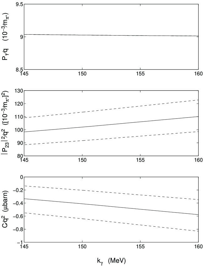
Figure 1: ChPT predicted behavior of the p waves. Solid line represents the predicted values and the dashed lines represent a $\pm$10% variation of $b_{p}$.

The predictions of ChPT for the ${\gamma}N\rightarrow{\pi}N$ reaction depend on three low energy constants labeled $b_{p}$, $a_{1}$, and $a_{2}$ [4]. Of these only $b_{p}$ effects the p wave multipoles. In Fig. 1 the variation of the three observables are also shown for a $\pm$10% variation of $b_{p}$. There is no dependence of $P_{1}$ on $b_{p}$. Furthermore, the slope of ${\mid}P_{23}\mid$ and C are approximately independent of $b_{p}$. The approximately linear deviation from the $q^{2}$ dependence of C and ${\mid}P_{23}{\mid}^{2}$, shown in Fig. 1, will be assumed in the analysis but with empirically determined constants.

We have performed three fits to the data. One uses the A, B, and C coefficients with the energy dependence of C specified as

$$C=q^{2}[\overline{C}+\widetilde{C}{\Delta}k_{\gamma}]$$ (7)

where ${\Delta}k_{\gamma}$ is taken for convenience to be in units of $m_{\pi^{0}}$.

A multipole fit was also performed with the functional form of the energy dependence of the p wave multipoles and $ImE_{0+}$ fixed. From the discussion of the expected energy dependence of the s and p wave multipoles the following energy dependence was chosen:

$$\begin{array}[]{c}\begin{array}[]{lr}ImE_{0+}=0&k<k_{T}(\pi^{+}n)\\ ImE_{0+}=\beta q_{+}&k>k_{T}(\pi^{+}n)\end{array}\\ P_{1}=q\overline{P_{1}}\\ {\mid}P_{23}{\mid}^{2}=q^{2}[\overline{P_{23}}+\widetilde{P_{23}}{\Delta}k_{\gamma}]\end{array}$$ (8)

where the fit parameters are the values of $ReE_{0+}(k_{i})$ at each photon energy, $\beta,\overline{P_{1}}$, $\overline{P_{23}}$,and $\widetilde{P_{23}}$.

We have also performed a unitary fit for which $E_{0+}(k_{\gamma})$ is parametrized as:

$$\begin{array}[]{c}E_{0+}(k_{\gamma})=A_{0}(k_{\gamma})+i\beta q_{+}\\ A_{0}(k_{\gamma})=\overline{A}+\widetilde{A}{\Delta}k_{\gamma}\end{array}$$ (9)

where the values of $\overline{A}$, $\widetilde{A}$, and $\beta$ were taken as free parameters.

To calculate the expected value of $\beta$ we use the best experimental value of $a(\pi^{-}p\rightarrow\pi^{0}n)=-(0.1301\pm 0.0059)/m_{\pi}$ from the observed width in the 1s state of pionic hydrogen atom [21]. This is in excellent agreement with ChPT predictions of $-(0.130\pm 0.006)/m_{\pi}$ [18]. Assuming isospin is conserved $a(\pi^{+}n\leftrightarrow\pi^{0}p)=-a(\pi^{-}p\leftrightarrow\pi^{0}n)$. There are no modern measurements for $E_{0+}({\gamma}p\rightarrow\pi^{+}n)$ so we can use the ChPT prediction of $28.2\pm 0.6$ [4, 14, 19]. From these one obtains $\beta=3.67\pm 0.18$ [14].

The analysis that will be presented here depends on the range of validity of Eq. (8). In order to insure that this analysis is accurate and as model independent as possible it will be terminated at a photon energy of 160 MeV. This is sufficient to show the main features of the threshold region.

3 Results

In this section the results of the analysis of the data [15] will be presented and compared with ChPT calculations [4]. The data were taken from threshold to 270 MeV. In the first publication only a preliminary analysis of the data to a photon energy of 152 MeV was presented [15]. In this publication a more thorough analysis to 160 MeV will be presented.

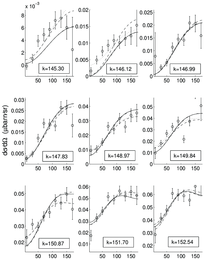
Figure 2: Differential cross sections (CM system) with statistical errors in ${\mu}b/sr$ versus pion angle in degrees. The photon energies in MeV are given. The solid line represents the unitary fit, dot-dot line the $A,B,\overline{C},\widetilde{C}$ fit, dash-dash line the multipole fit, and dash-dot line the ChPT fit.

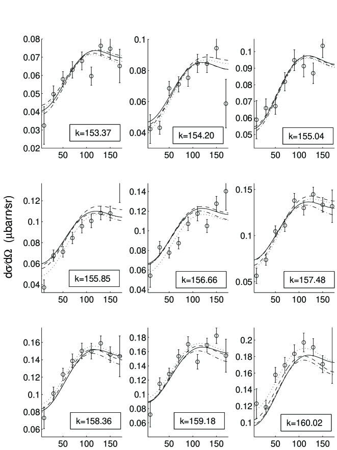
Figure 2: Continued.

The empirical fits and ChPT [4] results for $\sigma(\theta)$ are compared to experiment in Fig. 2. It should be pointed out that the errors shown in Fig. 2 are statistical only. The systematic errors are estimated to be approximately 5% [15]. For the A,B,C fit (Eq. (7)) the best fit values are $\overline{C}=-0.338\pm 0.025{\mu}b$, $\widetilde{C}=-1.83\pm 0.30{\mu}b$, and $\chi^{2}/DOF=1.65$. For ChPT [4] there are three low energy constants which were adjusted to obtain a best fit to the data. Qualitatively all of the fits and the ChPT calculation are very close with $\chi^{2}/DOF=1.96$ for the multipole fit and 2.21 for ChPT.

The fit parameters and $\chi^{2}$ results are shown in Table 2 and compared to ChPT. Only the fitting errors are presented. The values presented for ChPT [4] were obtained by fitting the numerical calculations with Eqs. (8) and (9) and finding the best fit parameters. The agreement between the fitted form and numerical results is excellent.

For the p wave multipoles one can see from Table 2 that the extracted values of $\overline{P_{1}}$ and $\overline{P_{23}}$ are in good agreement with ChPT [4]. In this part of the calculation there is only one low energy constant ($b_{p}$) which was fit to the data. On the other hand it can be seen that there is a large systematic error for $\widetilde{P_{23}}$. This can be seen by comparing the much different values obtained from the unitary and multipole fits. These results straddle the ChPT value. The fact that the next to leading order slope of the p wave multipoles is not strongly constrained by the data will have consequences in the determination of $ImE_{0+}$ (see Sec. 4).

The parameters for $ReE_{0+}$ ($\beta$, $\overline{A}$, and $\widetilde{A}$) are significantly different between the unitary fit and the ChPT calculation. As will be shown below (see Fig. 8 and discussion) the two resulting curves both are in reasonable agreement with the extracted values of $ReE_{0+}$ from the multipole fit. We should point out that for this multipole there are two low energy parameters ($a_{1}$ and $a_{2}$) that have been fit to the data.

Parameter	Unitary Fit	Multipole Fit	ChPT
$\chi^{2}/DOF$	2.13	1.96	2.21
$\beta$	$3.76\pm 0.11$	$2.82\pm 0.32$	$2.78$
$\overline{P_{1}}$	$9.006\pm 0.079$	$9.151\pm 0.071$	$8.998$
$\overline{P_{23}}$	$101.9\pm 1.1$	$95.40\pm 0.62$	$97.71$
$\widetilde{P_{23}}$	$41.8\pm 13.0$	$159.1\pm 7.3$	$108.5$
$\overline{A}$	$-0.12\pm 0.020$		-0.41
$\widetilde{A}$	$-4.27\pm 0.28$		-0.76

Table 2: Parameters in Eq. (8) and (9) for the Unitary and multipole fits and ChPT [4]. Except for $\chi^{2}$ all of the quoted parameters are given in units of $10^{-3}/m_{\pi^{+}}$. In Eqs. (8) and (9) $q$ and ${\Delta}k_{\gamma}$ are in units of $m_{\pi^{0}}$ and $q_{+}$ in units of $m_{\pi^{+}}$

The results for the total cross section are shown in Fig. 3. It can be seen that there is a discrepancy between the Saskatoon [16] and TAPS [15] results particularly for $k_{\gamma}>152$ MeV. The older Mainz results [8] tend to be in better agreement with the Saskatoon data. Unfortunately at this time the cause of this disagreement is not known.

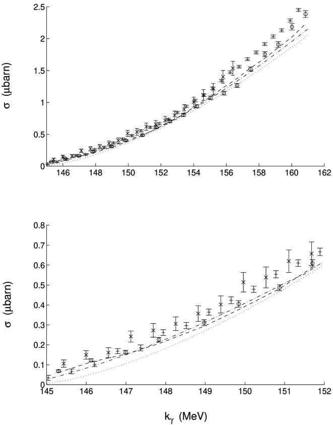
Figure 3: Measured total cross section with statistical errors in ${\mu}b$ versus photon energy with the ChPT calculations [4] and the empirical fits. The new Mainz (TAPS) data (circle) [15], Saskatoon (plus) [16], and older Mainz points (cross) [8] are shown. The bottom figure shows the energy region through the $\pi^{+}n$ threshold in more detail. In both figures dash-dash line represents the multipole fit, dash-dot line the ChPT result, and dot-dot line only the p wave contribution to the ChPT.

The Saskatoon group did not publish any differential cross section data. The only information that is presented is the “belt pattern” for the angular distributions. In order to use this information one has to perform a Monte Carlo calculation using predicted differential cross sections which are then compared with the “belt patterns”. We therefore cannot compare the results presented here for the differential cross sections with the Saskatoon data.

From Fig. 3 one can see that the ChPT fit is in good agreement with the TAPS data and not in agreement with the Saskatoon data. This is not surprising since the three free parameters of ChPT were fit to the TAPS data. One also notes that the p wave contribution to the total cross section is dominant except for the first few points above threshold. This makes it difficult to see the effect of the (s wave) unitary cusp in the cross section.

The results for the B coefficient are shown in Fig. 4. This shows the effect of the predicted unitary cusp because it is an sp interference amplitude. The extracted values of the B coefficient are in reasonable agreement with the unitary fit and with ChPT [4] because only the statistical errors are shown. An estimate of the systematic errors can be inferred from the scatter of the points.

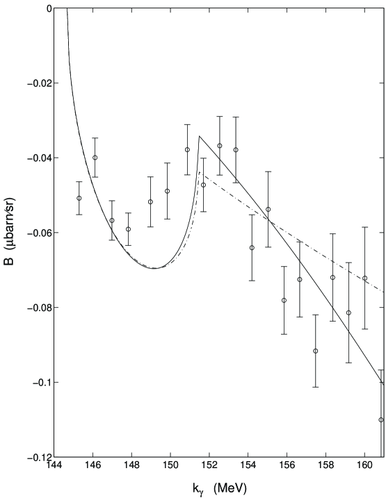
Figure 4: B coefficient (with statistical errors) vs. photon energy from fits and ChPT. Circles represent the $A,B,\overline{C}$ fit, solid line represents the unitary fit, and the dash-dot line the ChPT.

The results for the A coefficient are shown in Fig. 5. This is the most accurately measured coefficient since $\sigma(\theta=90^{\circ})=(q/k)A$ and also the total cross section is proportional to $A+C/3$ and ${\mid}C{\mid}\ll A$. As a consequence the errors for A are small. It can be seen, in contrast to the B coefficient, that the unitary cusp is hardly visible. This is due to the dominance of p waves as shown in Fig. 5. It can also be seen that ChPT calculation is in reasonable agreement with A.

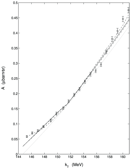
Figure 5: A coefficient (with statistical errors) vs. photon energy from fits and ChPT. Circles represent the $A,B,\overline{C}$ fit, solid line represents the unitary fit, dash-dash line the multipole fit, dash-dot line the ChPT, and dot-dot line the p wave contribution to ChPT.

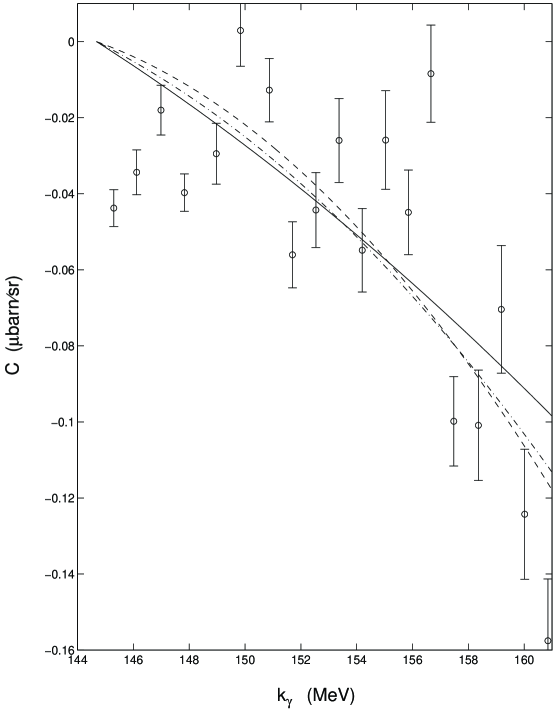
Figure 6: C coefficient (with statistical errors) vs. photon energy from fits and ChPT. Circles represent the $A,B,C$ fit, solid line represents the unitary fit, dash-dash line the multipole fit, and dash-dot line the ChPT.

The results for the C coefficient are shown in Fig. 6. It can be seen that all of the fits and the results of ChPT are in good agreement. In addition a fit in which the A, B, and C coefficients at each energy are found from a least square fit to the data are also presented. In this case the energy dependence of the C coefficient is not constrained by theory. The scatter of these C coefficients indicate that the data do not strongly constrain the p wave multipoles despite the fact that this is the dominant multipole in the unpolarized cross section. We conclude that although the present results are consistent with the ChPT theory calculations that the experiment with linearly polarized photons recently completed at Mainz [22] is needed for a more precise measurement of the p wave multipoles. The results from the analysis of this experiment will be available in the next year or two.

The extracted values of the magnitude of

$${\mid}E_{0+}{\mid}=\sqrt{(ReE_{0+})^{2}+(ImE_{0+})^{2}}$$

are shown in Fig. 7. These are obtained from the unitary fit to the Mainz/TAPS data [15] and from the published Saskatoon results [16]. Despite the discrepancy in the measured total cross sections, the two data sets result in values of ${\mid}E_{0+}{\mid}$ which are in reasonable agreement. The fitting errors for the unitary fit are significantly smaller than the errors shown for the individual points of the Saskatoon data since they represent an overall fit to the data.

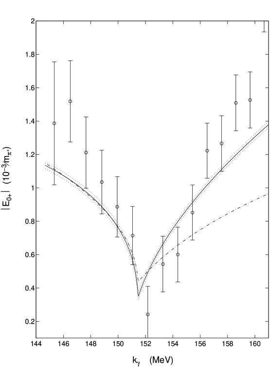
Figure 7: ${\mid}E_{0+}{\mid}$ vs. photon energy. Circles represent the Saskatoon data, solid line represents the unitary fit, dash-dot line the ChPT, and dot-dot lines represent the fitting errors of the unitary fit.

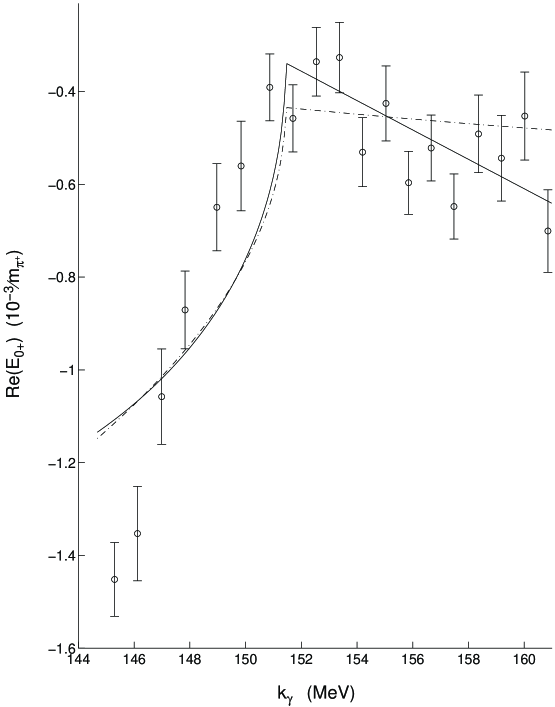
Figure 8: $ReE_{0+}$ vs. photon energy. The circles represent the multipole fit, the solid line represents the unitary fit, and the dash-dot line the ChPT fit.

The extrapolated threshold values for $E_{0+}$ are $-1.13\pm 0.04$ for the unitary fit and $-1.5\pm 0.1$ for the multipole fit in the usual units [14]. These two values do not agree because the two analyses give a somewhat different energy dependence for $E_{0+}$. If we take the average and adjust the error to reflect this disagreement the threshold value of $E_{0+}=-1.3\pm 0.2$ [14]. This is good agreement with the Saskatoon result of $-1.32\pm 0.1$ [14]. This disagrees with the older prediction of the low energy theorems [11, 12] of -2.28 [14] which have been shown to be incomplete [4, 12].

The $ReE_{0+}$ as extracted from the multipole fit is presented in Fig. 8. This agrees with the Saskatoon results [16] and the older Mainz results [8] within the experimental errors. The effect of the rapid energy variation of $ReE_{0+}$ below the $\pi^{+}n$ threshold is again visible in qualitative agreement with the ChPT calculation [4] and the unitary fit. Note that the errors shown in Fig. 8 are statistical only. The magnitude of the systematic errors can be inferred from the scatter of the points.

4 Model Dependence

The differential cross section for unpolarized photons in Eq. (2) shows that three independent combinations of the multipoles (A, B, and C) are measured while there are seven independent multipole parameters for the emission of s and p wave pions. In order to extract useful information about the multipoles from the data assumptions were made which follow from first principles which should cause relatively small analysis errors. In this section the sensitivity to these assumptions will be explored to obtain a measure of the uncertainties, and also to explore how future data, particularly with polarization degrees of freedom, can improve the situation.

The major model assumption that was made in this analysis is the assumption that the p wave multipoles have the same analytic energy dependence as predicted by ChPT [4]. In part this assumption has been checked by the fact that the least square parameters are close to those of ChPT (see Table 2). In order to further check this assumption an additional fit was made which was very similar to the multipole fit (Eq. 8) except that the p wave multipoles were assumed to vary linearly with $q$ (i.e. $\widetilde{P_{23}}=0$ in Eq. 8). This fit is quantitatively similar to those in which the p wave multipoles were assumed to vary as $qk$ [13]. The results of doing this can be surmised by the observation that A is the best measured of the three coefficients in Eq. (2) and by noting that this determines the absolute value of $E_{0+}$ in addition to the dominant p wave contribution. Since $ReE_{0+}$ is determined from the B coefficient this determines $ImE_{0+}$ after a suitable subtraction of the p wave contribution. If one assumes a smaller energy dependence in the p wave multipole then a stronger energy dependence will emerge for $ImE_{0+}$. The results for the determination of $ImE_{0+}$ are presented in Fig. 9 and it can be seen that this is precisely what has happened. For the fit in which the p waves are assumed to be proportional to $q$ the extracted value of $\beta=4.51\pm 0.20$, which is far larger then the value of $\beta=2.82\pm 0.32$ obtained with the multipole fit or $\beta=3.76\pm 0.11$ for the unitary fit. The two latter fits use the p wave energy dependence of Eq. (8). These results for $\beta$ indicate a strong correlation between $\beta$ and $\widetilde{P_{23}}$. This is to be expected since the only information about these parameters is obtained from A (see Eqs. 4 and 8).

Figure 9: $ImE_{0+}$ vs. photon energy. Solid line represents the unitary fit, dash-dash line the multipole fit, dash-dot line the ChPT, and dash-dash line the fit which assumes linear dependence of p waves of $q$.

From the spread in the values of $\beta$ shown in Fig. 9 and Table 2 one concludes that the systematic error is significantly larger then the fit error. This is due to the fact that there is not sufficient information in the unpolarized cross section to determine this quantity. Experiments with polarized targets are required to precisely determine $ImE_{0+}$ [6].

The cusp effect is isospin breaking due in part to the threshold difference between the $\pi^{0}p$ and $\pi^{+}n$ channels. In the ChPT calculation [4] isospin is broken by inserting the mass difference between the charged and neutron pions by hand. This leads to a value of $\beta=2.78$ which is significantly below the predicted value of $3.67\pm 0.19$ expected from the predicted values of $E_{0+}({\gamma}p\rightarrow\pi^{+}n)$ and $a(\pi^{+}n\leftrightarrow\pi^{0}p)$ quoted in Sec. 2. An improved ChPT calculation which takes isospin breaking into account in a more dynamic way seems to be required to obtain detailed agreement with experiment.

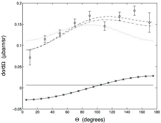
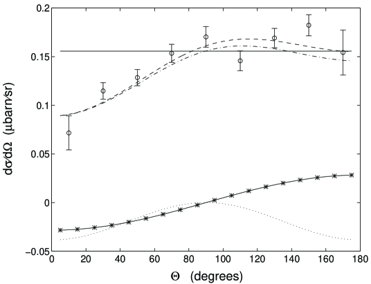
Figure 10: $\sigma(\theta)$ at 159.1 MeV showing the contributions of the A, B, and C terms (bottom) and s and p terms (top). In both graphs the circles represent Mainz/TAPS data, the dash-dash line represents the multipole fit, and the dash-dot line the ChPT fit. Solid line represents the s wave (top) and A term (bottom) contributions, the dot-dot line p wave (top) and C term (bottom) contributions, and stars represent sp (top) and B term (bottom) contributions to $\sigma(\theta)$.

It is also of interest to discuss how well the p wave multipoles are measured. By comparing the values obtained from the unitary and multipole fits (Table 2) it can be shown that the leading terms in the energy dependence of the p wave multipoles ($\overline{P_{1}}$ and $\overline{P_{23}}$ in Eq. (8)) are well determined, but not the next order term ($\widetilde{P_{23}}$ in Eq. (8)). This is a relatively small effect in the magnitude of the p waves as can be seen from the three curves for C in Fig. 6. The question of how accurately the energy dependence of the p wave multipoles can be obtained from the data can be seen by examining the relative contributions of the different contributions (Eqs. 2-4) to the differential cross section. As shown in Fig. 10 the p wave multipoles are dominant. However to extract their precise magnitude from the data is not trivial. First, as was discussed above, the best measured A coefficient has a tradeoff between $ImE_{0+}$ and the energy dependence of the p wave multipoles. The B coefficient is an interference term between $P_{1}$ and $ReE_{0+}$ so that only the product is determined. Only the relatively small C coefficient has purely p wave contributions. As was shown in the discussion of Fig. 6 this coefficient is poorly determined. The reason for this is illustrated in Fig. 10 which shows the contributions of the A, B, and C terms to $\sigma(\theta)$ at 159.1 MeV. This is a relatively high energy for this analysis so that the contribution of the C term is as large as possible. It can be seen that the C term contribution is relatively hard to determine with precision. It will be much better determined by the $\vec{\gamma}+p\rightarrow\pi^{0}+p$ reaction with linearly polarized photons [22]. In this case if one assumes that the $E_{1+}$ multipole is negligible the polarized photon asymmetry at $90^{\circ}$ is $-C/A$. This will be the most precise measurement of the energy dependence of the p wave multipoles.

5 Conclusions

We have presented a rigorous analysis of the recent TAPS/Mainz data [15]. Since there are three independent observables for the unpolarized cross section, while for s and p wave photo-pion emission there are seven independent amplitudes, some simplifying assumptions must be made. In this work these assumptions follow closely from first principles. The systematic errors of the analysis were assessed by using several assumptions; the main one is that the energy dependence of the p wave multipoles follow approximately the same analytic form predicted by ChPT [4].

The main conclusion is that the calculation of ChPT [4] are in reasonable agreement with the data. This one loop calculation has three low energy constants which are fitted to the data. The threshold value of $E_{0+}$ was determined to be $-1.3\pm 0.2$ in the usual units [14]. This is in agreement with the Saskatoon result of $-1.32\pm 0.1$ [16]. Note that this disagrees with the predictions of the older ”low energy theorems” of $-2.28$ [11, 12] which have been theoretically shown to be incomplete [4].

The predicted unitary cusp in the s wave electric dipole amplitude $E_{0+}$ [4, 5, 6], due to the two step ${\gamma}p\rightarrow\pi^{+}n\rightarrow\pi^{0}p$, has been observed in experiments at Mainz [8, 10, 15] and Saskatoon [16, 23]. Only a range of $\beta$ values (Eq. (1)) between approximately 2.8 and 4.5 [4] an be obtained from the unpolarized cross section data (Sec. 4).

The new experiments on the threshold ${\gamma}p\rightarrow\pi^{0}p$ reaction mark an important advance in our understanding of this important reaction. An understanding of the small discrepancy between the TAPS [15] and Saskatoon [16] results is important. A new experiment with linearly polarized photons has been performed [22] and we look forward to the completion of the data analysis to more completely test the ChPT predictions for the p wave multipoles [4]. Further work with polarized targets is required to precisely measure $\beta$, which should provide a measure of the s wave charge exchange scattering length $a_{cex}(\pi^{+}n\leftrightarrow\pi^{0}p)$ [6]. On the theoretical side we have seen tremendous progress in our understanding of threshold pion photo and electro production. Further advances are needed to treat isospin breaking in a better way and to test the convergence of $E_{0+}$.

References

- [1] See e.g. Dynamics of the Standard Model, J.F. Donoghue, E. Golowich, and B.R. Holstein, Cambridge University Press (1992).
- [2] S. Weinberg, Physica A96, 327 (1979). J. Gasser and H. Leutwyler, Ann. Phys. (N.Y.) 158, 142 (1984), Nucl. Phys. B250, 465 and 517 (1985).
- [3] For references and the present status of the field see: A.M. Bernstein and B. Holstein editors. Proceedings of the Workshop on Chiral Dynamics: Theory and Experiment. Springer Verlag, July 1995.
- [4] V. Bernard, N. Kaiser, and U.G. Meißner, Int. J. Mod. Phys. E4, 193 (1995), Nucl. Phys. B383, 442 (1992), Phys. Rev. Lett. 74, 3752 (1995), Z. für Physik C70, 483 (1996), Phys. Lett. B378, 337 (1996).
- [5] G. Fäldt, Nucl. Phys. A333, 357 (1980), J.M. Laget, Phys. Rep., 69, 1 (1981), A.N. Kamal, Phys. Rev. Lett., 63, 2346 (1989).
- [6] A.M. Bernstein, Newsletter No. 11, Dec. 1995 , Proceedings of the PANIC Conference (1996), in press, and to be published.
- [7] S. Weinberg, In Transactions of the N.Y. Academy of Science, Series II volume 38 (I.I.Rabi Festschrift), 185 (1977), and contribution in Ref. [3]. U. van Kolk, Ph.D. thesis, U. of Texas (1995) unpublished.
- [8] R. Beck et al., Phys. Rev. Lett. 65, 1841 (1990).
- [9] E. Mazzucato et. al. Phys. Rev. Lett., 57, 3144 (1986).
- [10] R. Beck in AIP Conference Proceedings No. 221, Particle Production Near Threshold (1990).
- [11] P. de Baenst, Nucl. Phys., B24, 633 (1970), A.I. Vainshtein and V.I. Zakharov, Sov. J. Nucl. Phys., 12, 333 (1971) and Nucl. Phys., B36, 589 (1972).
- [12] For critical discussion of the meaning of low energy theorems and a review of the literature see G. Ecker and U.G. Meißner, Comm. Nucl. Part. Phys., 21, 347 (1995).
- [13] A.M. Bernstein and B.R. Holstein, Comm. Nucl. Part. Phys., 20, 197 (1991), J.C. Bergstrom, Phys. Rev., C44, 1768 (1991), D. Drechsel and T. Tiator, J. Phys. G: Nucl, Part. Phys., 18, 449 (1992).
- [14] The values of the multipoles are quoted in the traditional units of .
- [15] M.Fuchs et al., Phys. Lett., B368, 20 (1996), M Fuchs, Ph.D. thesis, University of Gießen, (1996) unpublished.
- [16] J.C. Bergstrom et al., Phys. Rev. C53, R1052 (1996).
- [17] G. Höhler, Pion Nucleon Scattering, v. 9 of Landolt-Börnstein, Springer-Verlag, New York, 1983, Richard A. Arndt, John M. Ford, Zhujun Li, L. David Roper, Ron L. Workman, Phys. Rev. D., 43, 2131 (1991), and SAID program.
- [18] V. Bernard, N. Kaiser, and Ulf.G. Meißner, Phys. Lett. B309, 421 (1993).
- [19] V. Bernard, N. Kaiser, and Ulf.G. Meißner, Phys. Lett. in print [hep-ph/9603278].
- [20] E. Amaldi, S. Fubini, and G. Furlan, Pion Electroproduction, Springer Tracts in Modern Physics, 83 (1979).
- [21] D. Sigg et. al., Phys. Rev. Lett., 75, 3245 (1995), M. Janousch et. al., Proceedings of the PANIC Conference (1996) in press.
- [22] R. Beck et. al., recently completed TAPS experiment at Mainz.
- [23] J.C. Bergstrom, preprint submitted to the Newsletter.