DO PHASE TRANSITIONS SURVIVE BINOMIAL REDUCIBILITY AND THERMAL SCALING?

Abstract

First order phase transitions are described in terms of the microcanonical and canonical ensemble, with special attention to finite size effects. Difficulties in interpreting a “caloric curve” are discussed. A robust parameter indicating phase coexistence (univariance) or single phase (bivariance) is extracted for charge distributions.

1 Phase transitions, phase coexistence, and charge distributions

Since the early studies of complex fragment emission at intermediate energies, a “liquid vapor phase transition” had been claimed as an explanation for the observed power law dependence of the fragment charge distribution. The basis for such claims was the Fisher droplet theory [1] which was advanced to explain/predict the clusterization of monomers in vapor. According to this theory, the probability of a cluster of size $m$ is given by:

$$P(m)\propto e^{\frac{-(\mu_{L}-\mu_{V})m}{kT}}m^{-\tau}e^{\frac{-c_{s}m^{2/3}}{kT}}$$ (1)

where $\mu_{L}$, $\mu_{V}$ are the liquid and vapor chemical potentials, $\tau$ is the Fisher critical exponent, $c_{s}$ the surface energy coefficient for the liquid. For $\mu_{V}>\mu_{L}$ the liquid phase is stable and large clusters are found. For $\mu_{V}<\mu_{L}$ the vapor is stable and small clusters are present. At the critical temperature the liquid-vapor distinction ends, $\mu_{L}=\mu_{V}$ and the surface energy coefficient vanishes. The cluster size distribution assumes a characteristic power law dependence.

A recent analysis of very detailed experiments has claimed not only the demonstration of a near critical regime, but also the determination of other critical coefficients [2] besides $\tau$.

Another recent announcement claiming the discovery of a first order phase transition associated with multifragmentation [3] has created a vast resonance. Because of the greater simplicity inherent to this subject and because of its relevance to some of our studies, we discuss it here in some detail.

This study claims to have determined the “caloric curve” (sic) of a nucleus, namely the dependence of nuclear temperature on excitation energy. The temperature is determined from isotopic ratios (e.g. ³He⁴He, ⁶Li⁷Li), while the excitation energy is determined through energy balance. The highlight of this measurement is the discovery of a plateau, or region of constant temperature, which is considered indicative of a first order phase transition from liquid to vapor phase.

Apparently, the “paradigm” the authors have in mind is a standard picture of the diagram temperature $T$ vs enthalpy $H$ for a one component system at constant pressure $P$.

It is not clear whether this experimental curve can be interpreted in terms of equilibrium thermodynamics. If this is the case, several problems arise. For instance, the claimed distinction between the initial rise (interpreted as the fusion-evaporation regime) and the plateau (hinted at as the liquid-vapor phase transition) is not tenable, since evaporation is the liquid-vapor phase transition, and no thermodynamic difference exists between evaporation and boiling.

Furthermore, the “caloric curve” requires for its interpretation an additional relationship between the variables $T$, $P$, and $V$. More to the point, the plateau is a very specific feature of the constant pressure condition rather than being a general indicator of a phase transition. For instance, a constant-volume liquid-vapor phase transition is not characterized by a plateau but by a monotonic rise in temperature. This can be easily proven by means of the Clapeyron equation, together with the ideal-gas equation for the vapor.

For the nearly ideal-vapor phase ($P=nT$), we write $dP=Tdn+ndT$ where $n$ is the vapor molar density. In order to stay on the univariance line, we need the Clapeyron equation: $dP/dT=\Delta H/(T\Delta V)$ where $\Delta H$ is the molar enthalpy of vaporization and $\Delta V$ is the molar change in volume from liquid to gas. From this we obtain: $n\left(\Delta H-T\right)dT=T^{2}dn$. At constant pressure $dn$=0, so $dT$=0. For $dn>0$, we see immediately that $dT>0$. Using $dE\approx dn\Delta E$, where $\Delta E$ is the molar heat of vaporization at constant volume, we finally obtain:

$$\left.\frac{\partial T}{\partial E}\right|_{V}\approx\frac{T^{2}}{n\Delta E^{2}}=\frac{1}{n\Delta S^{2}}.$$ (2)

The positive value of this derivative shows that the phase transition at constant volume is characterized by a monotonic increase in temperature.

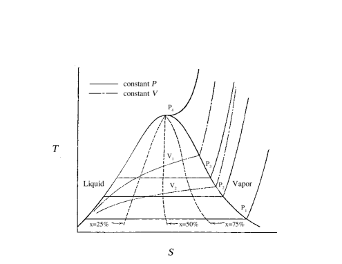
Figure 1: Temperature-entropy diagram for steam. Curves are shown for constant pressure ($P_{4}>P_{3}>P_{2}>P_{1}$), constant volume ($V_{1}<V_{2}$) and constant percentage in the gas phase (dashed lines).

As an example, Fig. 1 shows a standard temperature $T$ vs entropy $S$ diagram for water vapor. The region under the bell is the phase coexistence region. For the constant pressure curves ($\Delta S=\Delta H/T$), the initial rise along the “liquid” curve is associated with pure liquid, the plateau with the liquid-vapor phases, and the final rise with overheated vapor. The constant volume curves, however, ($\Delta S=\Delta E/T$) cut across the coexistence region at an angle, without evidence for a plateau.

Thus the reminiscence of the observed “caloric curve” with “the paradigm of a phase transition” may be more pictorial than substantive, and indicators other than the plateau may be needed to substantiate a possible transition from one to two phases. More specifically, an additional relationship between the three variables $P,T,V$ (like $P$=const, or $V$=const, etc.) is needed to interpret a $T$-$E$ diagram unequivocally.

2 Triviality of first order phase transitions

The great attention to the alleged discovery of first order phase transition in nuclei would suggest that such a phenomenon may be of great significance to our understanding of nuclear systems. In fact, it is easy to show that first order phase transitions are completely trivial. Here are the reasons:

1)If there are two or more phases known or even hypothetically describable, then there will be first order phase transitions.

2) The thermodynamics of these transitions is completely determined by the thermodynamical properties of each individual isolated phase. These phases do not affect each other, and do not need to be in contact.

As an example, let us consider Fig. 2, where the molar free energy $F$ at constant $T$ is plotted vs the molar volume for a liquid and the gas phase. Stability of each phase requires each of these curves to be concave. In the region between the points of contact of the common tangent, the free energy is minimized by apportioning the system between the liquid and gas phase. Each phase is defined at the point of tangency, and the segment of the tangent between the two points is the actual free energy of the mixed phase. The slope of the common tangent is the negative of the constant pressure at which the transition takes place. The coexistence region is completely defined by the properties of the liquid at $V_{L}^{M}$ and and of the gas at $V_{G}^{M}$. Consequently, it is irrelevant whether the liquid is in contact with the vapor or not!

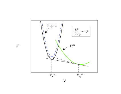
Figure 2: The free energy as a function of molar volume for a liquid and gas. The dashed lines refer to a drop rather than to bulk liquid.

This discussion applies to infinite phases. However, it is simple to introduce finite size effects, e.g. surface effects.

The pressure of a drop is always greater than that of the infinite liquid. In Fig. 2 the common tangent (dashed) becomes steeper, in accordance with the increased free energy of the liquid.

3 Microcanonical or Canonical Ensemble?

Any good textbook of statistical mechanics contains the demonstration that, in the thermodynamic limit, all ensembles are equivalent, i.e. they give the same thermodynamic functions.

In dealing with phase transitions in finite systems one may question whether this equivalence is retained. Let us review the connection between, for instance, the Microcanonical and the Canonical Ensemble.

Let $\rho(E)$ be the microcanonical level density. The corresponding canonical partition function is the Laplace transform

$$Z(\beta)=\sum e^{-\beta E_{i}}\approx\int\rho(E)e^{-\beta E}dE$$ (3)

The partition function is usually easier to calculate than the level density. However, the latter can be obtained from the former through the inverse Laplace Transform.

$$\rho(E)=\frac{1}{2\pi i}\int{\Large\circ}Z(\beta)e^{\beta E}d\beta$$ (4)

We can write Eq. (4) as

$$S_{{\rm Micro}}=\ln\rho(E)=\ln Z_{0}+\beta_{0}E-\frac{1}{2}\ln\left(2\pi\left.\frac{\partial^{2}\ln Z}{\partial\beta^{2}}\right|_{\beta_{0}}\right)$$ (5)

where $\beta_{0}$ corresponds to the stationary point of the integrand. Furthermore,

$$S_{{\rm Micro}}=S_{{\rm Can}}-\ln\left(2\pi\left.\frac{\partial^{2}\ln Z_{0}}{\partial\beta^{2}}\right|_{\beta_{0}}\right)$$ (6)

The first term to the right is of order $N$ while the second is of order $\ln N$.

When $N$ goes to infinity (thermodynamic limit) one can disregard the term of order $\ln N$. For finite $N$ one can easily evaluate the correction term which turns out to be very accurate even for small $N$. For instance, consider a percolation system with $N$ bonds of which $n$ are broken. As an example of a finite system, let us take $N$=6 and $n$=3. The exact expression yield $\rho$=20. The saddle point approximation yields $\rho$=20.6! One can see that with little additional effort one can retain the use of the partition function with little loss of accuracy even for the smallest systems!

Still, in the mind of physicists there is the bias that a microcanonical approach, or its equivalent through the inverse Laplace Transform of the Partition Function, is more correct than the canonical approach because the former conserves energy, while the latter does not.

In fact the microcanonical distribution is given by

$$P(E)=\delta\left(E(p,q)-E_{0}\right).$$ (7)

The canonical distribution instead is given by

$$P(E)=Ke^{-\beta E(p,q)}.$$ (8)

In this case, there are energy fluctuations.

So, which is ultimately the “right” ensemble? If it does not matter, as in the the thermodynamic limit, the point is moot. But for finite systems it matters. However, consider the case of a small system which is a part of a larger system. Let us call the total energy $E$ and that of the small system $\epsilon$. Then

$$S(E,\epsilon) = S(E,0)+\left.\frac{\partial S}{\partial\epsilon}\right|_{\epsilon=0}\epsilon+...$$ (9)

$$= S(E,0)-\frac{\epsilon}{T}+...$$

Thus

$$\rho(E,\epsilon)\approx\rho(E,0)e^{-\epsilon/T}.$$ (10)

The energy of the small system is canonically distributed, in a real, physical sense. The canonical, or grand canonical distribution very frequently has a direct physical reality and is not an approximation to a “more correct” microcanonical distribution. For instance, Na clusters in thermal equilibrium with a carrier gas are canonically distributed in energy.

What is the relevance of the above to phase transitions? There are claims that a microcanonical approach yields “sharper” phase transitions than a canonical approach, because of its lack of energy fluctuations. However, any thermodynamic property, including phase transitions, is defined in statistical mechanics as an ensemble average. Thus the resulting properties are not properties of the system alone, but they are properties of the ensemble. So with reference to phase transitions in particular, arguments like “the microcanonical ensemble yield sharper phase transitions compared to the canonical ensemble, and because of that it is better” are meaningless. If the physical ensemble is canonical, the canonical description is the correct one, irrespective of whether it is sharper or fuzzier than the microcanonical description.

4 Sharpness of phases and phase transitions

Let us consider the free energy of the liquid phase in Fig. 2. We can expand about the minimum as follows:

$$F=F_{0}+\frac{1}{2}\left.\frac{\partial^{2}F}{\partial V^{2}}\right|_{\widehat{V}}(\Delta V)^{2}.$$ (11)

The probability of volume fluctuations are then

$$P(V)\propto\exp\left[-\frac{(\Delta V)^{2}}{2\sigma_{V}^{2}}\right]$$ (12)

where $1/\sigma_{V}^{2}=\left.\partial^{2}F/\partial V^{2}\right|_{\widehat{V}}$. Since $F\propto N$, $\sigma_{V}^{2}\propto 1/N$. Therefore important volume (density) fluctuations are to be expected at small $N$. A cluster, or a nucleus, which are not kept artificially at constant density, are going to fluctuate substantially in density.

At coexistence, the correlated fluctuations between the two phases make the sharpness of the phases and of the phase transition even more washed out.

5 A robust indicator of phase coexistence

As we have seen, a “generic” caloric curve of the kind obtained in ref. [3] is of problematic interpretation because of the difficulty in establishing the additional relation $F(V,T,P)$ associated with the evolution of the system.

On the other hand, theoretical predictions of multifragmentation phase transitions on the basis of calculated discontinuities in the specific heat are suspicious because these calculations are performed at constant volume!

Furthermore, the only meaningful experimental question about phase transitions is whether the system is present in a single phase or there is phase coexistence. In thermodynamical language, we want to know whether the system is monovariant (two phases) or bivariant (one phase).

We have found a robust indicator for just these features in the charge distributions observed in multifragmentation.

The charge distributions depend both on the number $n$ of fragments in the events, and on the excitation energy, measured through the transverse energy $E_{t}$ [4, 5].

It is possible empirically to “reduce” the charge distributions for $n$ fragments to that of just one, and to “scale” the transverse energy effect by means of the following empirical equation

$$\sqrt{E_{t}}\left(\ln P_{n}(Z)+ncZ\right)=-F(Z)$$ (13)

where $F(Z)$ is a universal function of $Z$, and $c$ is a constant. This empirical equation suggests that the charge distributions can be expressed as:

$$P_{n}(Z)\propto e^{-\frac{B(Z)}{T}-ncZ}.$$ (14)

The first term in the exponent was interpreted [4, 5] as an energy or enthalpy term, associated with the energy (enthalpy) needed to form a fragment. The second term was claimed to point to an asymptotic entropy associated with the combinatorial structure of multifragmentation. It was observed that a term of this form arises naturally in the charge distribution obtained by the least biased breaking of an integer $Z_{0}$ into $n$ fragments [4]. Such a $Z$ distribution is given approximately by:

$$P(Z)=\frac{n^{2}}{Z_{0}}e^{-\frac{nZ}{Z_{0}}}=cn^{2}e^{-cnZ}.$$ (15)

While this form obviously implies charge conservation, it is not necessary that charge conservation be implemented as suggested by Eq. (15). In fact it is easy to envisage a regime where the quantity $c$ should be zero. Sequential thermal emission is a case in point. Since any fragment does not know how many other fragments will follow its emission, its charge distribution can not reflect the requirement of an unbiased partition of the total charge among $n$ fragments.

On the other hand, in a simultaneous emission controlled by a $n$-fragment transition state [6], fragments would be strongly aware of each other, and would reflect such an awareness through the charge distribution.

The question then arises whether $c=0$ or $c>0$, or even better, whether one can identify a transition from a regime for which $c=0$ to a new regime for which $c>0$. To answer this question, we have studied the charge distributions as a function of fragment multiplicity $n$ and transverse energy $E_{t}$ for a number of systems and excitation energies. Specifically, we present data for the reaction ³⁶Ar+¹⁹⁷Au at $E/A$=80 and 110 MeV and the reaction ¹²⁹Xe+¹⁹⁷Au at $E/A$=50 and 60 MeV in Fig. 3.

Figure 3: Plots of the coefficient $c$ versus $E_{t}$ for the reactions ¹²⁹Xe+¹⁹⁷Au at $E/A$=50 and 60 MeV (top panel) and ³⁶Ar+¹⁹⁷Au at $E/A$=80 and 110 MeV (bottom panel). The error bars are statistical.

It is interesting to notice that for all reactions and bombarding energies the quantity $c$ starts at or near zero, it increases with increasing $E_{t}$ for small $E_{t}$ values, and seems to saturate to a constant value at large $E_{t}$.

This behavior can be compared to that of a fluid crossing from the region of liquid-vapor coexistence (univariant system) to the region of overheated and unsaturated vapor (bivariant system). In the coexistence region, the properties of the saturated vapor cannot depend on the total mass of fluid. The presence of the liquid phase guarantees mass conservation at all average densities for any given temperature. Hence the vapor properties, and, in particular, the cluster size distributions cannot reflect the total mass or even the mean density of the system. In our notation, $c=0$.

On the other hand, in the region of unsaturated vapor, there is no liquid to insure mass conservation. Thus the vapor itself must take care of this conservation, at least grand canonically. In our notation, $c>0$. In other words we can associate $c=0$ with thermodynamic univariance, and $c>0$ with bivariance.

To test these ideas in finite systems, we have considered a finite percolating system and a system evaporating according to a thermal binomial scheme [7, 8]. Percolation calculations [9] were performed for systems of $Z_{0}$=97, 160 and 400 as a function of the percentage of bonds broken ($p_{b}$). Values of $c$ were extracted as a function of $p_{b}$.

The results are shown in Fig. 4. For values of $p_{b}$ smaller than the critical (percolating) value ($p_{b}^{crit}\approx$ 0.75 for an infinite system), we find $c=0$. This is the region in which a large (percolating) cluster is present. As $p_{b}$ goes above its critical value, the value of $c$ increases, and eventually saturates in a way very similar to that observed experimentally.

Figure 4: top: A plot of $cZ_{0}$ versus the percentage of broken bonds $p_{b}$ from a percolation calculation [9] for three systems $Z_{0}$=97 (circles), $Z_{0}$=160 (squares) and $Z_{0}$=400 (diamonds). bottom: A plot of $cZ_{0}$ versus excitation energy per nucleon from a binomial evaporation calculation [8] for ⁶⁴Cu and ¹²⁹Xe. The statistical error bars are shown for errors larger than the symbol size.

Notice that although the phase transition in the infinite system is second order at $p=p_{c}$, here the region for which $c=0$ mimics a first order phase transition.

An evaporation calculation was also carried out for the nuclei ⁶⁴Cu and ¹²⁹Xe according to the thermal binomial scheme [7, 8]. The only constraint introduced was to prevent at every step the emission of fragments larger than the available source. The resulting charge distributions are very well reproduced by Eq.(14). The extracted quantity $cZ_{0}$ is plotted in the bottom panel of Fig. 4 as a function of excitation energy per nucleon. In both cases $cZ_{0}$ goes from 0 to a positive finite value (equal for both nuclei) as the energy increases. The region where $c=0$ is readily identified with the region where a large residue survives. On the other hand when $c>0$ there is no surviving residue.

These results are in striking agreement with those obtained for percolation. For both kinds of finite systems, the univariant regime ($c=0$) is associated with the presence of a residue while the bivariant regime ($c>0$) with the absence of a residue.

This work was supported by the Director, Office of Energy Research, Office of High Energy and Nuclear Physics, Nuclear Physics Division of the US Department of Energy, under contract DE-AC03-76SF00098.

6 References

References

- [1] M. E. Fischer, Rep. Prog. Phys. 67, 615 (1967).
- [2] M. L. Gilkes et al., Phys. Rev. Lett. 73, 1590 (1994).
- [3] J. Pochodzalla et al., Phys. Rev. Lett. 75, 1040 (1995).
- [4] L. Phair et al., Phys. Rev. Lett. 75, 213 (1995).
- [5] L.G. Moretto et al., Phys. Rev. Lett. 76, 372 (1996).
- [6] J.A. Lopez and J. Randrup, Nucl. Phys. A 512, 345 (1990).
- [7] L.G. Moretto et al., Phys. Rev. Lett. 74, 1530 (1995).
- [8] R. Ghetti et al., to be published.
- [9] W. Bauer, Phys. Rev. C 38, 1297 (1988).