Neutron density distributions from antiprotonic ${}^{208}\mbox{Pb}$ and ${}^{209}\mbox{Bi}$ atoms

Abstract

The X-ray cascade from antiprotonic atoms was studied for ${}^{208}\mbox{Pb}$ and ${}^{209}\mbox{Bi}$. Widths and shifts of the levels due to the strong interaction were determined. Using modern antiproton-nucleus optical potentials the neutron densities in the nuclear periphery were deduced. Assuming two parameter Fermi distributions (2pF) describing the proton and neutron densities the neutron rms radii were deduced for both nuclei. The difference of neutron and proton rms radii $\Delta r_{np}$ equal to $0.16\pm(0.02)_{stat}\pm(0.04)_{syst}$ fm for ${}^{208}\mbox{Pb}$ and $0.14\pm(0.04)_{stat}\pm(0.04)_{syst}$ fm for ${}^{209}\mbox{Bi}$ were determined and the assigned systematic errors are discussed. The $\Delta r_{np}$ values and the deduced shapes of the neutron distributions are compared with mean field model calculations.

I Introduction

Beginning more than ten years ago, we have performed an experimental study of the medium-heavy and heavy antiprotonic atoms using the slow antiproton beam from the Low Energy Antiproton Ring (LEAR) at CERN. The main objective of our program was to obtain information on the neutron distribution at the nuclear periphery and to provide data useful for deducing the antiproton-nucleus optical potential parameters.

Two experimental methods were employed. First, using the so called “radiochemical method” we have investigated Jastrzȩbski et al. (1993); Lubiński et al. (1994, 1998); Schmidt et al. (1999) the ratios of peripheral neutron to proton densities at distances around 2.5 fm larger than the nuclear charge half-density radius Wycech et al. (1996). The method consisted in measuring the yield of radioactive nuclei having one proton or one neutron less than the target nucleus, produced after antiproton capture, cascade and annihilation in the target antiprotonic atom. The experiment yielded 19 density ratios (proportional to the “halo factor” $f_{\mathrm{halo}}$ defined below), which were subsequently employed to deduce the shape of the peripheral neutron distribution.

The second method consisted in measurements of the antiprotonic-atom level widths and shifts due to the strong antiproton-nucleus interaction. These observables are sensitive to the interaction potential which contains, in its simplest form, a term depending on the sum of the neutron and proton densities. The level widths and in a number of cases also the level shifts were measured for 34 antiprotonic atoms (in some cases for different isotopes of the same element).

The rich harvest of the two methods employed which are sensitive to the neutron and proton density ratio and the sum of these densities, has allowed to derive a number of systematic conclusions on the nuclear periphery properties presented in a series of summary and analysis publications Trzcińska et al. (2001a, b); Jastrzȩbski et al. (2004); Trzcińska et al. (2004). Moreover, our data were used to determine the antiproton-nucleus optical model parameters through global fits of $\bar{\mbox{p}}$ X-rays and halo factors Friedman et al. (2005); S. Wycech. F.J. Hartmann, J. Jastrzȩbski, B. Kłos, A. Trzcińska, T. von Egidy, to be published. with a substantially larger and more precise database than employed in previous approaches Batty et al. (1995, 1997).

Besides our summary papers, after the end of the antiprotonic X-ray (PS209) experiment, we prepared more detailed reports, containing information on experimental procedures and their analysis for some cases studied Schmidt et al. (1998); Hartmann et al. (2001); Schmidt et al. (2003); Kłos et al. (2004). The present article, dealing with ${}^{208}\mbox{Pb}$ and ${}^{209}\mbox{Bi}$ antiprotonic atoms, is the next in this series.

During the last years it was shown that properties of the ${}^{208}\mbox{Pb}$ neutron distribution can be correlated with a number of quantities in various fields. In particular the knowledge of the difference $\Delta r_{np}$ between the rms radii of neutrons and protons in this nucleus constrains the symmetry energy of nuclear matter and therefore is reflected in the neutron Equation of State (EOS) Brown (2000); Furnstahl (2002); Dieperink et al. (2003); Steiner et al. (2005); Yoshida and Sagawa (2006); Steiner and Li (2005). The neutron EOS models, in turn, are used to calculate the properties of neutron stars, such as their radii and proton fraction Horowitz and Piekarewicz (2001a, b). However, not only the first moments of the neutron density distributions, but also their shapes are of considerable interest, e.g. in the determination of the isovector potential parameter of the pion-nucleus s-wave interaction in nuclear matter Geissel et al. (2002) or in the calculation of the lepton flavor violating muon-electron conversion rate Kitano et al. (2002). There is also a certain dependence on the radial neutron distribution in the proposed determination of the ${}^{208}\mbox{Pb}$ neutron rms radius through parity violating electron-nucleus scattering Horowitz et al. (2001).

Experimentally, the $\Delta r_{np}$ value in ${}^{208}\mbox{Pb}$ was previously determined using hadronic probes (elastic scattering, inelastic scattering exciting GDR), reported in Refs. Ray (1979); Hoffmann et al. (1980); Krasznahorkay et al. (1994, 1999); Starodubsky and Hintz (1994); Csatlós et al. (2003); Krasznahorkay et al. (2004); Karataglidis et al. (2002) and discussed in Jastrzȩbski et al. (2004). There were also some attempts to deduce higher moments of the neutron distribution from the hadron scattering experiments Mack et al. (1995) (see also Karataglidis et al. (2002)). On the other hand, the ability of the medium-energy elastic proton scattering data to determine the neutron distributions was recently contested Piekarewicz and Weppner (2006).

The measurement in ${}^{209}\mbox{Bi}$ offers other advantages. It is the only experiment that allows to see an even-odd isotopic effect in heavier nuclei, in this case due to the loosely bound proton in ${}^{209}\mbox{Bi}$. One difficulty in the way of analysis is the calculation of the hyperfine-structure that is comparable to the strong interaction shift and broadening. After this is done, it turns out that the level shift in ${}^{208}\mbox{Pb}$ is repulsive (as most of the lower shifts), but the level shift in ${}^{209}\mbox{Bi}$ is attractive. This finding is open to interpretation. Here we pursue the view that it is related to a $\bar{\mbox{p}}$N quasi-bound state, which is important in cases of loosely bound valence nucleons.

II Experimental methods

The heavy antiprotonic atoms ²⁰⁸Pb and ²⁰⁹Bi were investigated during the experiment PS209 at CERN in 1996 using antiprotons of momentum 106 MeV/c. Table 1 gives the target properties and the number of antiprotons used for each target.

The antiprotonic X-rays emitted during the antiproton cascade were measured by three high-purity germanium (HPGe) detectors. Two detectors were coaxial with an active diameter of 49 mm and a length of 50 mm (relative efficiency about 19% and 17%, respectively), and the third one was planar with 36 mm diameter and a thickness of 14 mm. The detectors were placed at distances of about 50 cm from the target at angles of 13^∘, 35^∘ and 49^∘ towards the beam axis, respectively. The detector-target distance was adjusted to obtain a good signal-to-noise ratio and to decrease at the same time the background produced by pions from the annihilation processes.

More details concerning the experimental methods, the detector calibration and the data reduction may be found in our previous publications Schmidt et al. (1998); Hartmann et al. (2001); Schmidt et al. (2003); Kłos et al. (2004).

III Experimental results

The strong interaction between antiproton and nucleus causes a sizeable change of the energy of the last X-ray transition from its purely electromagnetic value. The nuclear absorption reduces the lifetime of the lowest accessible atomic state (the “lower level”, which for lead is the $(n,l=9,8)$ state) and hence this X-ray line is broadened. Nuclear absorption also occurs from the next higher level (“upper level”) although the effect on level energy and width is generally too small to be directly measured. The width of the $(n,l=10,9)$ level was deduced indirectly by measuring the intensity loss of the final X-ray transitions. The level scheme for the antiprotonic Pb atom with the observables of the X-ray experiment is shown in Fig. 1.

The X-ray spectrum measured with antiprotons stopped in ²⁰⁸Pb is shown in Fig. 2. Those lines in the spectra that are not broadened were fitted with Gaussian profiles. The lowest observable LS-split doublet lines $(n=10\to 9)$, which are significantly broadened, were fitted with two Lorentzians convoluted with Gaussians (Fig. 3).

The measured relative intensities of the antiprotonic X-rays observed in the investigated lead and bismuth targets are given in Table LABEL:relat. These intensities were used to determine the feeding of the consecutive $n$ levels along the antiprotonic-atom cascade. This is shown for ${}^{208}\mbox{Pb}$ in Fig. 4.

Table 3 gives the measured shifts $\varepsilon$, defined by $\varepsilon=E_{\mathrm{em}}-E_{\mathrm{exp}}$, where $E_{\mathrm{exp}}$ the experimental value for the transition energy and $E_{\mathrm{em}}$ the energy calculated without strong interaction Borie (1983). For the lead $(n,l=9,8)$ levels the shifts are clearly repulsive, whereas for bismuth the levels shifts are consistent, within the errors, with zero (Fig. 5). However, as discussed in the next sections, there exists an additional repulsive shift due to the hyper fine structure. For the $(n,l=10,9)$ levels in lead the shifts are repulsive, as in the case of the $(n,l=9,8)$ levels, but the shifts are smaller. Tables 4 and 5 give the measured widths. As indicated above, the widths of the $(n,l=10,9)$ levels were derived from the intensity balance of transitions feeding and depopulating these levels. Contributions of parallel transitions to the measured intensities were obtained from cascade calculations (see Schmidt et al. (1998)). The rates for radiative dipole transitions were calculated with the formulae given in Ref. Eisenberg and Kessler (1961). The Auger rates were derived from the radiative rates and from cross sections for photoeffect using Ferrell’s formula Ferrell (1960). The width of the levels $(n,l=10,9)$ are larger for ${}^{209}\mbox{Bi}$ than for ${}^{208}\mbox{Pb}$ (Fig. 5). This is due to the hyperfine structure in Bi, which will be discussed below.

IV Analysis and discussion of the ${}^{208}\mbox{Pb}$ measurement

IV.1 Introductory statements

The analysis of the presented antiprotonic ${}^{208}\mbox{Pb}$ atom data is based on some assumptions that are briefly mentioned here and discussed below. We assume and show by a comparison with model calculations that charge, proton and neutron distributions in this nucleus can be well approximated by two-parameter Fermi (2pF) distributions: $\rho(r)=\rho_{0}\cdot\{1+\mathrm{exp}(\frac{r-c}{a})\}^{-1}$, where $c$ is the half-density radius, $a$ is the diffuseness parameter, and $\rho_{0}$ is a normalization factor. In particular, calculating the neutron rms radius from the antiprotonic X-ray data sensitive to densities at distances around 1.5 fm larger than the half-density charge radius Wycech et al. (1996), we extrapolate the experimental density well into the interior of the nucleus. As shown below (Sec. IV.3), this assumption is in reasonable agreement with the density shapes calculated in terms of the mean field models.

In evaluating the observables of the antiproton-nucleus interaction the important question of the ratio of the annihilation probability on a neutron to the one on a proton arises. In the simplest nuclear optical potentials this ratio is given by the ratio of the imaginary parts of the effective scattering lengths, $R=Im\,b_{0}^{\;n}/Im\,b_{0}^{\;p}$. The experimental determination of this quantity Bugg et al. (1973); Wade and Lind (1976) gave $R=0.63$.

In spite of this observation, a value R=1 was assumed in the optical potentials proposed in Refs. Batty et al. (1995, 1997); Friedman et al. (2005). Our analysis of the antiprotonic X-ray data, together with the radiochemical experiment, also indicated A. Trzcińska, Ph.D. Thesis, Warsaw University, 2001 () (unpublished) a better consistency of these two methods when $R=1$ was chosen. Therefore this value is also adopted in the present data evaluation, as discussed in the following sections.

IV.2 Charge and proton distributions

It is generally assumed (see e.g. Ref. Fricke et al. (1995)) that the charge rms values are known for the stable nuclei with remarkable precision, about 0.3%. The same belief is often projected on the charge distributions. In Fig. 6 we show (as it was already observed in Kłos et al. (2004)) that this is not the case for the radial distances where the antiproton-nucleus interaction takes place in ${}^{208}\mbox{Pb}$ (about 7 to 10 fm away from the nuclear center, see below). In this figure the charge density of ${}^{208}\mbox{Pb}$, tabulated in a number of compilations, is compared with the most recent one by Fricke et al. Fricke et al. (1995). Neglecting the oldest tabulation, differences of up to 50% are observed between Fricke et al., Jager et al. de Jager et al. (1974) and de Vries et al. de Vries et al. (1987) for radial distances close to 10 fm. We consequently use the Fricke charge distribution in this work.

Experiments using electromagnetically interacting probes give charge density distributions or rms charge radius values (e.g. Fricke et al. (1995); de Vries et al. (1987)) whereas point proton distributions are needed when Batty’s zero-range antiproton-nucleus optical potential Batty et al. (1995) is used for the analysis of the experimental data. For the finite-range version of the $\bar{\mbox{p}}$-nucleus potential Friedman et al. (2005); S. Wycech. F.J. Hartmann, J. Jastrzȩbski, B. Kłos, A. Trzcińska, T. von Egidy, to be published. these point distributions are folded over an interaction range.

In Ref. Oset et al. (1990) the analytical formulae to transform the 2pF charge distribution to the 2pF point distributions of the proton centers were presented. We have previously used them in our data analysis, presented e.g. in Ref. Trzcińska et al. (2001b). Similar analytical formulae were recently given in Ref. Patterson and Peterson (2003). In order to transform the ${}^{208}\mbox{Pb}$ proton charge distribution of Ref. Fricke et al. (1995), we have used the proton charge rms radius $\sqrt{<r_{p}^{2}>}=0.875$ fm cod , obtaining 2pF point proton parameters of $c_{p}=6.684$ fm, $a_{p}=0.446$ fm and rms $r_{p}=5.436$ fm.

IV.3 Calculated mean field neutron and proton distributions

The proton and neutron distributions in the doubly magic ${}^{208}\mbox{Pb}$ nucleus were subject of a large number of theoretical investigations. In this paper we select Skyrme-Hartree-Fock (HF) and the Hartree-Fock-Bogoliubov models, namely those with the SkP (HFB) Dobaczewski et al. (1984) and SkX (HF)  Brown (1998) parametrization, both reproducing the ${}^{208}\mbox{Pb}$ charge (proton) radius and neutron binding energy remarkably well. (It has, however, recently been shown that the SkP Skyrme model may diverge for some nuclei if calculated to sufficient accuracy Lesinski et al. (2006)). The third self-consistent mean filed model considered here belongs to the framework of the relativistic mean field theory (RMF) with the recent DD-ME2 parametrization of the effective interaction Lalazissis et al. (2005). Although in fitting the DD-ME2 parameters the ${}^{208}\mbox{Pb}$ $\Delta r_{np}$ value (of 0.20 fm) was used to adjust the interaction parameters, the shape of the neutron distribution was obtained from the calculation.

Figure 7, left panel, presents the proton and neutron distributions of ${}^{208}\mbox{Pb}$ as calculated using the DD-ME2 parametrization. This and two other distributions were approximated by 2pF distributions fitted to the theoretical densities. Satisfactory fits were achieved for radii between 1 and 10 fm (local differences between theoretical and fitted densities were less than 10% for protons and less than 4% for neutrons in the radius range 2–9 fm, Fig. 7, right panel). Figure 8 shows the summed neutron and proton densities for the three forces considered. The relationship between the neutron densities, rms radius and equation of state is being investigated with a larger set of mean-field models in B. A. Brown and G. Shen and G. C. Hillhouse and J. Meng, unpublished .

Table 6 gives the results of the fitting procedure. The rms radii calculated using $a$ and $c$ values of the 2pF are close to those obtained using the theoretical distributions directly. The neutron distributions are close to the “halo type” Trzcińska et al. (2001b), with $\Delta c_{np}=0.02$ fm for SkP, $\Delta c_{np}=0.07$ fm for SkX and $\Delta c_{np}$=0.05 fm for DD-ME2, respectively. This is illustrated in the left-hand part of  Fig. 9, showing the normalized neutron to proton density ratio obtained from the density distributions of the discussed models. The figure presents also the “pure halo” distribution with $\Delta r_{np}$=0.16 fm and $\Delta c_{np}$=0 fm.

IV.4 Antiproton-nucleus optical potentials

The standard potential for hadronic atoms Batty et al. (1997) are composed of two terms

$$V^{opt}=V_{S}(r)+{\bf\nabla}V_{P}(r){\bf\nabla}$$ (1)

involving proton and neutron components. Both terms, the local $V_{S}$ and the gradient $V_{P}$ are expected to have the folded form

$$V_{S,P}(r)=\frac{2\pi}{\mu_{N\overline{N}}}b_{S,P}\int d{\bf u}f({\bf u})\rho({\bf r}-{\bf u}),$$ (2)

which involves nucleon densities $\rho$, folded with a (usually Gaussian) function $f$ of some rms radius ,$r_{range}$, of the range, ”effective lengths ” $b$, and some weak dependence of the reduced mass ${\mu_{N\overline{N}}}$ on nuclear recoil. It turned out already in a first analysis for heavy atoms Batty et al. (1997) that an independent determination of $b_{S}$ and $b_{P}$ is not realistic. A simplified result in Ref. Batty et al. (1997) gave $b_{S}=-2.5(3)-i\,3.4(0.3)$ fm with zero $r_{range}$, which we call the Batty potential and use in our calculations. The recent phenomenological best fit (Friedman potential) is obtained with a single term of $b_{S}\,(=b_{0})=-1.3(1)-i\,1.9(1)$ fm for both neutrons and protons and $r_{range}=1.04$ fm Friedman et al. (2005). Within all these calculations the X-ray data suggested no significant differences in the the values of the p$\bar{\mbox{p}}$ and n$\bar{\mbox{p}}$ lengths. No relation of the phenomenological $b_{S}$ to the $N\bar{N}$ scattering parameters has been established. Another recent analysis S. Wycech. F.J. Hartmann, J. Jastrzȩbski, B. Kłos, A. Trzcińska, T. von Egidy, to be published. attempts to find such a relation from the analysis of the lightest atoms H, D, He and of scattering data described in terms of the Paris $N\bar{N}$ potential. One important difference arises in equation (2), which also contains nucleon recoil terms not required in a phenomenological approach. The nucleon recoil term constitutes about a quarter of the total potential and depends on the state of the nucleon. This leads to a more complicated parametrization, which will not be repeated here. In this potential S. Wycech. F.J. Hartmann, J. Jastrzȩbski, B. Kłos, A. Trzcińska, T. von Egidy, to be published. one obtains roughly $b_{S}=-1.7-i\,0.9$ fm, $b_{P}=0-i\,0.4$ fm³ with $r_{range}=0.8$ fm and the absorptive part of these parameters compares well with the p$\bar{\mbox{p}}$ and p$\bar{\mbox{n}}$ scattering data.

Presently available optical potentials are unable to reproduce the level shifts in Pb. This reflects a more general difficulty related to uncertainties of the real part of $V^{opt}$. More specific difficulties such as $\bar{\mbox{p}}$N-quasi-bound states or long-range pion exchange forces in the $\bar{\mbox{p}}$N system have already been discussed in Refs. Wycech (2001); S. Wycech. F.J. Hartmann, J. Jastrzȩbski, B. Kłos, A. Trzcińska, T. von Egidy, to be published. .

IV.5 Annihilation probability

The probability $P_{n,l}(r)$ of the nuclear capture from a given atomic state $(n,l)$ is defined (for local optical potentials) as $P_{n,l}(r)=\mid\phi_{n,l}(r)\mid^{2}(Im\,V^{opt})\cdot r^{2}$, where $\phi_{n,l}$ is the antiprotonic wave function and $r$ is the radial distance from the nuclear center.

The most probable value of this probability was calculated for some cases in Ref. Wycech et al. (1996) and the results of these calculations were confirmed by the analysis given in Ref. Friedman et al. (2005). The calculations of the $P_{n,l}(r)$ distributions for ${}^{208}\mbox{Pb}$ were preformed using Batty potential and density distributions discussed in Sec. IV.3. Figure 10 shows this annihilation probability distributions for DD-ME2 densities and Table 7 gives parameters of this distribution. Wider distributions (by about 60% for upper level and 20% for lower level) with more pronounced tails for larger radii are obtained using finite range optical potentials.

IV.6 Interpolated halo factor

In our previous analysis of the antiprotonic X-ray and radiochemical data the crucial information used in deducing the shape of the neutron distribution (“halo type” or “skin type”, see Trzcińska et al. (2001b) for the definition) was the experimentally determined halo factor $f_{\mathrm{halo}}=\frac{Y(N_{t}-1)}{Y(Z_{t}-1)}\cdot\frac{Z_{t}}{N_{t}}\cdot R$; here $Y$ are the yields for the $A_{t}-1$ nuclei, $Z_{t}$, $N_{t}$ and $A_{t}$ are the target proton, neutron and mass numbers, respectively, and $R$ was defined and discussed above. We have shown previously that in a number of cases for which this halo factor could be measured, it indicated that the corresponding 2pF neutron distribution is close to the “halo type”, i.e. with equal proton and neutron radius parameter ($c_{n}$=$c_{p}$) and larger diffuseness parameter for neutrons ($a_{n}$$>$$a_{p}$). Again, this observation is in fair agreement with the mean-field calculations of the nuclear densities (see Sec. IV.3).

In the case of the ${}^{208}\mbox{Pb}$ nucleus, the experimental determination of the halo factor by the radiochemical method was not possible as one of the ($A_{t}-1$) isotopes (${}^{207}\mbox{Pb}$) is not radioactive. In order to have at least some indication of its value the ${}^{208}\mbox{Pb}$ halo factor was deduced by interpolation between $f_{\mathrm{halo}}$ values for other nuclei, which are plotted either as a function of the neutron binding energy Lubiński et al. (1994) (see Fig. 11) or of the asymmetry parameter $\delta=(N-Z)/Z$  J. Jastrzȩbski, A. Trzcińska, P. Lubiński, F.J. Hartmann, R. Schmidt, T. von Egidy, B. Kłos . (Note that, as discussed in Ref. Trzcińska et al. (2001b), the halo factors published by us before this reference should be multiplied by 0.63). The interpolated $f_{\mathrm{halo}}$ for ${}^{208}\mbox{Pb}$ found in this way is $2.8\pm 0.4$.

This interpolated value can be compared with the results of Bugg et al. Bugg et al. (1973), where the idea of the neutron halo factor was introduced for the first time to interpret the ratio of charged pions generated by antiproton annihilation in various targets, including ${}^{208}\mbox{Pb}$. In that work the halo factor, defined as $f^{\pi}_{halo}=\frac{N(n{\bar{p}})}{N(p{\bar{p}})}\frac{Z}{N}\,R$ (where $N(n{\bar{p}})$ and $N(p{\bar{p}})$ are the number of $\bar{\mbox{p}}$ annihilations on peripheral neutrons and protons, respectively) was measured for the ${}^{208}\mbox{Pb}$ nucleus by detecting the charged pions emitted after antiproton capture in nuclei Bugg et al. (1973). The result obtained, $f^{\pi}_{halo}=2.34(50)$, is based on the assumption that $R=0.63$, with this latter number extracted from the $\bar{\mbox{p}}$ capture in carbon. The result has been subject to some criticism for neglecting the final state interactions and a possible dependence of $R$ on the actual nucleus. The more recent Obelix experiments determined $R=0.48(3)$ from low-energy capture in He Balestra et al. (1989), while the best fit optical potential requires $R\approx 1$ Friedman et al. (2005). This discrepancy is resolved if one realizes that capture in He involves mostly S-waves and capture from high angular momentum states in heavier nuclei involves mostly P (or higher) waves in the $N\bar{N}$ system S. Wycech, Proceedings of ”PHYSICS WITH ULTRA SLOW ANTIPROTON BEAMS” Workshop, AIP 2005, vol. 793, p. 201 . We refer to Ref. S. Wycech, Proceedings of ”PHYSICS WITH ULTRA SLOW ANTIPROTON BEAMS” Workshop, AIP 2005, vol. 793, p. 201 for some details of the calculation, which estimates $R\approx 0.9-1.0$ in the lead region and for a new analysis of the Bugg result. $R=1$ is used in these calculations. This yields $f^{\pi}_{halo}(\mathrm{Pb})=1.8(4)$. One can obtain the average radius of the absorption $r^{\pi}$ via calculations of the final state pion interactions and comparison of the final experimental and calculated pion spectra. This yields $r^{\pi}=c_{ch}+1.35$ fm.

IV.7 Experimental results analyzed by optical potentials

IV.7.1 The zero $N\overline{N}$ range antiproton-nucleus potential of Batty

Our previous results Trzcińska et al. (2001b) for the neutron distribution in ${}^{208}\mbox{Pb}$ were obtained using a zero-range $N\overline{N}$ force Batty potential Batty et al. (1995, 1997). This potential, obtained by a fit to the antiprotonic X-ray data mainly on light nuclei was determined before our results were published. It has, therefore, the evident philosophical advantage when compared to the recently published potentials strongly S. Wycech. F.J. Hartmann, J. Jastrzȩbski, B. Kłos, A. Trzcińska, T. von Egidy, to be published. or completely Friedman et al. (2005) relying on our results, including the ${}^{208}\mbox{Pb}$ nucleus.

The neutron-distribution parameters deduced using Batty’s potential are shown in Table 6. Calculations were done with a code based on the work by Leon Leon and Seki (1974). The $\Delta r_{np}$ is calculated as the difference between the rms radii of the corresponding 2pF point proton (Fricke) and point neutron distributions under the assumption of a “halo type” distribution ($\Delta c_{np}$=0). The $\Delta r_{np}$ value of 0.16 fm differs by 0.01 fm from the previously published one Trzcińska et al. (2001b); this is due to the updated value cod of the electromagnetic proton rms radius used in the transformation from charge to proton densities.

As indicated above, our experimental data yield $\Delta r_{np}=0.16$ fm under the assumption of $c_{n}=c_{p}$. In Figs. 12 and 13 we show how the relaxation of this condition would influence the difference of the Fermi-distribution parameters and the rms radii difference for the ${}^{208}\mbox{Pb}$ nucleus.

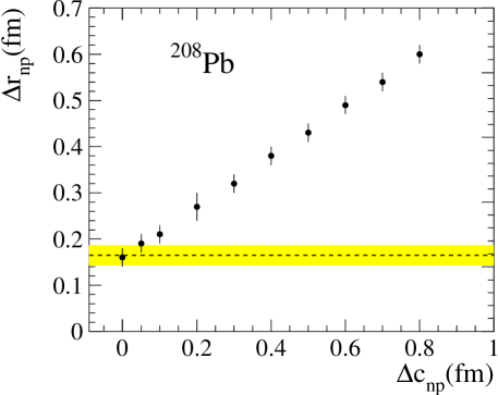
Figure 13: The relation between the difference of the neutron and proton half-density radii $\Delta c_{np}$ and the deduced difference between rms radii of neutron and proton distributions $\Delta r_{np}$ of ${}^{208}\mbox{Pb}$ for the zero-range interaction Batty potential. The dashed line and shaded region shows the weighted average and the error, respectively, of $\Delta r_{np}$ determined in the hadron scattering experiments (see Ref. Jastrzȩbski et al. (2004)).

The data in Fig. 12 present the change of $\Delta a_{np}$ when we allow the $\Delta c_{np}$ to change while still being in agreement with the experimental level widths. It is seen that with the extreme neutron-skin assumption (identical proton and neutron diffuseness, $\Delta a_{np}$=0) the neutron-proton difference of the half density radii $\Delta c_{np}$ should be close to 0.8 fm. As shown in Fig. 13 such a large value of this difference would lead to $\Delta r_{np}$ close to 0.6 fm.

In Ref. Jastrzȩbski et al. (2004) we have discussed the results for $\Delta r_{np}$ in ${}^{208}\mbox{Pb}$ obtained by using hadron scattering data. The weighted average of six experimental results, obtained between 1979 and 2003, is $\Delta r_{np}=0.16\pm 0.02$ fm Jastrzȩbski et al. (2004). It is in excellent agreement with the result obtained from the antiprotonic X-rays with the zero interaction range Batty potential. The gray band in Fig. 13 indicates the error margin of the weighted average of the hadron scattering experiments, allowing a difference in the $\Delta c_{np}$ value between the 2pF distribution of neutrons and protons in ${}^{208}\mbox{Pb}$ to be 0.08 fm at most.

The upper limit for $\Delta c_{np}$ can also be estimated comparing the calculated neutron to proton density ratio with the interpolated halo factor of ${}^{208}\mbox{Pb}$. This density ratio is plotted in the right panel of Fig. 9 as a function of the radius for $\Delta r_{np}$=0.16 fm (Batty potential X-ray value for $\Delta c_{np}$=0 and average value from the hadron scattering data). Two halo factors are shown in this figure: one resulting from the pion emission experiment and the other one from the interpolation (see Sec. IV.6). Although the pion experiment is not limiting the $\Delta c_{np}$ value, the interpolated $f_{\mathrm{halo}}$ clearly indicates that $\Delta c_{np}$ has to be smaller than 0.1 fm. This determines the systematic error of the $\Delta r_{np}$ value to be equal to 0.04 fm. If Ref. de Jager et al. (1974) instead of Ref. Fricke et al. (1995) is taken for the charge distribution, $\Delta r_{np}$=0.12 fm is obtained, i.e. the systematic error is also 0.04 fm for this case (cf. also results of Ref. S. Wycech. F.J. Hartmann, J. Jastrzȩbski, B. Kłos, A. Trzcińska, T. von Egidy, to be published. in Sec. IV.7.3).

The assigned statistical and systematic error for the $\Delta r_{np}$ value indicates about 1% uncertainty in the determination of the neutron rms radius in ${}^{208}\mbox{Pb}$ from the antiprotonic atom data. This value is comparable to the expected precision of the parity violation measurements Horowitz et al. (2001) of this quantity.

The comparison of the experimentally determined level widths and shift with the theoretical proton and neutron distributions (see Sec. IV.3) using Batty’s potential is shown in Table 8. The level widths calculated with the SkP and SkX distributions are too small (by 12% and 27%, respectively) whereas the DD-ME2 distributions result in widths close to the experimental values. As indicated in Sec IV.4, the value of the shift is not reproduced for any theoretical distribution.

It is interesting to note that the SkX interaction with the value closest to the experimental $\Delta r_{np}$ leads to level widths which are clearly below the observed ones. It indicates that for this interaction the nucleon density decreases too fast with $r$. This was illustrated in Fig. 8 by a comparison of the summed neutron and proton densities for the three forces considered. As previously discussed in Karataglidis et al. (2002), too small proton but especially neutron diffuseness exhibited by the SkX model is the reason for this behavior (cf. Table 6). Our antiprotonic atom data presented in Table 8 are therefore a confirmation of the conclusions drawn from the analysis of nucleon elastic scattering, presented in Ref. Karataglidis et al. (2002).

IV.7.2 The finite $N\overline{N}$ range potential of Friedman

Contrary to the Batty potential Batty et al. (1995, 1997), the finite-range antiproton-nucleus interaction potential recently proposed by Friedman et al. Friedman et al. (2005) was based almost completely on the PS209 experimental data, including the antiprotonic atom level widths and shifts of ${}^{208}\mbox{Pb}$ and ${}^{209}\mbox{Bi}$ reported in this publication.

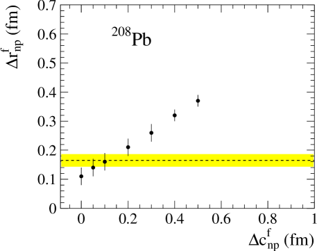
Figure 15: The same as Fig. 13, but for the finite-range Friedman potential Friedman et al. (2005).

In order to obtain a similar relationship as that shown for Batty’s potential in Fig. 12, the 2pF distribution of protons (see Table 6) was folded over the interaction range with 1.04 fm rms radius. The (folded) neutron density was fitted using the optical potential parameters from Friedman et al. (2005) to the experimental level widths of ${}^{208}\mbox{Pb}$, varying $\Delta c^{f}_{np}$. The $\Delta a^{f}_{np}$ values of the folded densities were deduced from the fit and are shown in Fig. 14. Figure 15, similar to Fig. 13, shows the resulting $\Delta r^{f}_{np}$ values of the folded density distributions as a function of the folded $\Delta c^{f}_{np}$ values.

It can be shown that the transformation from the point-like nucleon distributions to the folded ones increases the $\Delta a^{f}_{np}$ values by about 15%, leaving $\Delta c_{np}$ and $\Delta r_{np}$ approximately unchanged. Therefore, without any supplementary conditions these results indicate that using the finite-range version of the optical potential as proposed by Friedman et al. (2005), the $\Delta r^{f}_{np}$$\approx$$\Delta r_{np}$ value obtained for ${}^{208}\mbox{Pb}$ is between 0.11 fm ($\Delta c^{f}_{np}$=0 fm) and 0.38 fm ($\Delta c^{f}_{np}$=0.54 fm).

In Ref. Friedman et al. (2005) it was shown that if all antiprotonic data are presented in the form $\Delta r_{np}=\alpha(N-Z)/A+\beta$ Trzcińska et al. (2001b) the global fit to these data allows $\alpha$ values between 0.9 fm and 1.3 fm (our previous data in Trzcińska et al. (2004) analyzed in terms of the point proton optical potential gave $\alpha=0.90\pm 0.15$ fm). This $\alpha$ range gives $\Delta r_{np}$ values between 0.154 fm and 0.240 fm.

Another limit of the $\Delta r_{np}$ values could be obtained with the help of the weighted average of the hadron scattering data, giving $\Delta r_{np}$=0.16$\pm$0.02 fm Jastrzȩbski et al. (2004). Two standard deviations of this average (cf. Fig. 15) put the lower and upper limit of the $\Delta r_{np}$ as 0.12 fm and 0.20 fm.

Taking the lower allowed value from the global fit and the upper one from the hadron scattering gives $\Delta r^{f}_{np}$$\approx$$\Delta r_{np}$=0.17 fm as the result of the finite range Friedman potential with the estimated error of $\pm$0.02 fm.

This result implies $\Delta c^{f}_{np}$$\approx$$\Delta c_{np}$ of 0.13 fm, i.e. the neutron distribution essentially of the “halo type” but with a small contribution of the “skin type”. Such a distribution is shown in Fig. 9 by the curve labeled “G”, which lies slightly below the lower limit of the interpolated halo factor.

The comparison of the experimentally determined level widths and shift with the theoretical proton and neutron distributions using the Friedman potential is given in the lowest part of Table 8. The calculated level widths have about 5% uncertainty due to the folding procedure applied. Within these errors calculated level widths are identical to those obtained using Batty’s potential.

IV.7.3 A constraint finite $N\overline{N}$ range potential

A parallel study with the potential from Ref. S. Wycech. F.J. Hartmann, J. Jastrzȩbski, B. Kłos, A. Trzcińska, T. von Egidy, to be published. generates two solutions $\Delta r_{np}$=0.16(3) fm for the electron scattering charge de Jager et al. (1974) and/or $\Delta r_{np}$=0.22(3) fm for the muonic charge density Fricke et al. (1995). These solutions favor halo type neutron densities, both are characterized by large $\chi^{2}$ values due to the poorly reproduced level shift.

V Analysis and discussion of ${}^{209}\mbox{Bi}$ data

Since the ${}^{209}\mbox{Bi}$ nucleus has the spin $I=9/2$ and magnetic moment $\mu=4.08\cdot\mu_{N}$ (where $\mu_{N}$ is the nuclear magneton), the antiprotonic atom levels are split. The related hyperfine shifts are smaller than the fine structure (f.s.) splitting but comparable to the strong interaction shifts. The standard formula H.A. Bethe and E. E. Salpeter, Handbuch der Physik, vol. XXXV, Springer, Berlin 1956 , extended to the case of an anomalous magnetic moment Barmo et al. (1981), gives

$$E_{hfs}=\frac{\alpha g_{\bar{p}}g_{Bi}}{8mM}\frac{[F(F+1)-J(J+1)-I(I+1)]}{J(J+1)n^{3}(l+1/2)}(mZ\alpha)^{3},$$ (3)

where $M$ is the proton mass, $m$ is the reduced mass, $gI=\mu$ in nuclear magnetons. The last transition in Bi is split into 10 dominant components in the upper f.s. state and into 9 components in the lower f.s. components. These correspond to different values of the total spin of the system $F=J+I,...,J-I$. Assuming a statistical population $\sim(2F+1)$, the observed spectral line becomes asymmetrical. One obtains an overall 50 eV repulsive shift of the centroid and an additional ”broadening” of 150 eV. This yields a lower width of 350(50) eV and an attractive lower shift of 37(53) eV, generated by strong interaction. (The upper level width averaged over the fine structure components (see Table 5) is equal to 6.9(1.3) eV). One thus faces a sizable isotopic effect between attraction in ²⁰⁹Bi and repulsion in ²⁰⁸ Pb atoms. The difference is related to the weakly bound valence proton in this Bi isotope. As discussed on previous occasions, there are indications of a quasi-bound state in the p$\bar{\mbox{p}}$ system just below the threshold. Such a state generates few distinct cases of an anomalous behavior of level shifts in nuclei with loosely bound nucleons Wycech (2001). For a more quantitative discussion of these phenomena we refer to a parallel publication S. Wycech. F.J. Hartmann, J. Jastrzȩbski, B. Kłos, A. Trzcińska, T. von Egidy, to be published. .

Assuming (as for ${}^{208}\mbox{Pb}$) $\Delta c_{np}$=0 fm, the difference of the neutron and proton diffuseness parameter was fitted to level widths using Batty’s potential. The $\Delta r_{np}$ value obtained is equal to 0.14$\pm$0.04 fm, lower by 0.04 fm than the previously published one Trzcińska et al. (2001b). In Ref. Trzcińska et al. (2001b) the hyperfine splitting of the lower level discussed above was not taken into account.

VI Summary and conclusions

In this article we have presented an analysis of the nuclear structure information extracted from the studies of the antiprotonic atoms $\bar{\mbox{p}}$-${}^{208}\mbox{Pb}$ and $\bar{\mbox{p}}$-${}^{209}\mbox{Bi}$. The experimentally determined level widths and shifts of these atoms at the end of the antiprotonic cascade depend on the antiproton-nucleus interaction potential. In turn, the crucial ingredient of this potential is the nucleon density at the radial distance where the antiproton-nucleus interaction occurs. Therefore, as it was shown already in our first publications in this series Jastrzȩbski et al. (1993); Lubiński et al. (1994), the study of antiprotonic atoms may constitute a powerful tool for the extraction of information on the properties of the nuclear periphery.

In the analysis of the antiprotonic atom data presented here we have been essentially using two optical antiproton-nucleus potentials, proposed by Batty et al. Batty et al. (1995, 1997) and Friedman et al. Friedman et al. (2005), respectively. The Batty potential, now more than ten years old, was obtained by fitting the potential parameters to the 33 level widths and 15 level shifts of antiprotonic atoms published at that time, mainly of light and a few intermediate-mass nuclei. The fits were performed with a zero-range antiproton-nucleon interaction. Although this unphysical assumption is presently avoided Friedman et al. (2005); S. Wycech. F.J. Hartmann, J. Jastrzȩbski, B. Kłos, A. Trzcińska, T. von Egidy, to be published. as leading to worse fits than the finite range potentials, we still pursue our data analysis using the Batty prescription in its simplest form. Our arguments are that although “point nucleon distributions” and “zero range interaction potentials” are probably an oversimplification, the obtained parameters are deduced from the fit to the experimental data. It may be expected that this fact somehow in an automatic way introduces the corrections of the method deficiencies. Moreover, as already mentioned at the beginning of Sec. IV.7.1, the Batty-potential parameters were obtained before our antiprotonic atom data were available, ensuring the interpretation of the results to be independent of the interpretation tools.

Recently, an antiproton-nucleus optical potential with finite interaction range was proposed by Friedman et al. Friedman et al. (2005). It was shown that the 90 data points from our PS209 X-ray experiments, together with 17 data points from the radiochemical experiment, determine an attractive and absorptive $\bar{\mbox{p}}$-nuclear isoscalar potential, which fits the data well.

However, as the ${}^{208}\mbox{Pb}$ antiprotonic X-ray data were used in the determination of the Friedman potential, we have tried to show in the analysis of the experiment with this potential what can be deduced on the neutron distribution of this nucleus on a more general ground. To this end we have used the information on the trend of the $\Delta r_{np}$ values as a function of the asymmetry parameters $(N-Z)/A$, allowed by the potential of Ref. Friedman et al. (2005), and previously analyzed Jastrzȩbski et al. (2004) results of the hadron scattering experiments.

Another fit with a finite-range potential was recently proposed (Ref. S. Wycech. F.J. Hartmann, J. Jastrzȩbski, B. Kłos, A. Trzcińska, T. von Egidy, to be published. , see also Sec. IV.7.3). The reader is referred to the original reference for the discussion of the global fit to the antiprotonic X-ray data performed and the $\Delta r_{np}$ values deduced for ${}^{208}\mbox{Pb}$. These values are used in the present publication to estimate the systematic errors.

It was shown in this paper that by an analysis based strictly on the experimental antiprotonic level widths one would be unable to propose meaningful limits for the $\Delta r_{np}$ value in ${}^{208}\mbox{Pb}$. Applying the Batty potential with a pure “halo shape” of the neutron distribution ($\Delta c_{np}$=0 fm) leads to $\Delta r_{np}$=0.16 fm. The lowest limit of the interpolated halo factor would allow at most $\Delta c_{np}$=0.1 fm, i.e. $\Delta r_{np}$=0.20 fm, similarly to the $2\sigma$ uncertainty of the average $\Delta r_{np}$ value deduced from the hadron scattering experiments. The analyzed theoretical proton and neutron distributions using HF, HFB and RMF models give a $\Delta c_{np}$ value of 0.07 fm at most. If the charge distribution from Ref. de Jager et al. (1974) is used instead of that from Ref. Fricke et al. (1995), $\Delta r_{np}$=0.12 fm is obtained. We conclude that our experiment interpreted using Batty’s potential with the supplementary information given above leads to $\Delta r_{np}$=$0.16\pm(0.02)_{stat}\pm(0.04)_{syst}$ fm in the ${}^{208}\mbox{Pb}$ nucleus. A value for $\Delta r_{np}$ that is only 0.01 fm larger is deduced from the analysis using the Friedman potential.

Significant results were obtained applying the Batty and Friedman potentials with the theoretical proton and neutron distributions to get the antiprotonic ${}^{208}\mbox{Pb}$ atom level widths and shift. As it was discussed in Sec. IV.4 the experimental level shift was not reproduced. On the other hand for each theoretical distribution both potentials give almost identical widths in spite of the fact that one is “zero range” and the other one is “finite range” interaction potential. The calculated widths are smaller in some cases than the experimental ones. This is interpreted as evidence obtained from antiprotonic atoms for too rapid a decrease of these theoretical nucleon densities as a function of the radial distance due to a too small diffuseness of these densities. A similar conclusion was previously obtained from the analysis of nucleon elastic scattering.

Tables

Table 1: Target properties and number of antiprotons used.

Target	thickness d	enrichment	number of $\bar{p}$ (108)
	(mg/cm2)	(%)
208Pb	130.4	99.1	17
209Bi	132.7	nat.	1.4

Table 2: Measured relative X-ray intensities, normalized to the transition n = 13 $\to$ 12 (average value from three detectors).

Transition	208Pb	209Bi
10$\to$ 9	69.0 $\pm$ 2.3	63.6 $\pm$ 3.3
11$\to$ 10	99.6 $\pm$ 3.2	97.8 $\pm$ 3.6
12$\to$ 11	103.8 $\pm$ 4.1	102.1 $\pm$ 4.7
13$\to$ 12	100.0 $\pm$ 4.6	100.0 $\pm$ 4.9
14$\to$ 13	93.5 $\pm$ 5.0	93.8 $\pm$ 5.4
15$\to$ 14	81.3 $\pm$ 3.7	81.2 $\pm$ 4.0
16$\to$ 15	59.4 $\pm$ 2.7	61.4 $\pm$ 3.1
17$\to$ 16	54.8 $\pm$ 10.9∗	80.3 $\pm$ 10.4∗
18$\to$ 17	73.4 $\pm$ 3.6	71.2 $\pm$ 4.0
19$\to$ 18	56.0 $\pm$ 2.6	56.6 $\pm$ 2.9
20$\to$ 19	48.2 $\pm$ 2.3	53.4 $\pm$ 4.8
21$\to$ 20	44.9 $\pm$ 3.3	67.8 $\pm$ 6.3
11$\to$ 9	3.3 $\pm$ 0.3
12$\to$ 10	7.6 $\pm$ 0.5	5.3 $\pm$ 0.8
13$\to$ 11	10.1 $\pm$ 0.3	9.1 $\pm$ 0.5
14$\to$ 12	11.2 $\pm$ 0.6	10.4 $\pm$ 0.8
15$\to$ 13	10.6 $\pm$ 0.5	11.2 $\pm$ 0.8
16$\to$ 14	10.5 $\pm$ 0.5	10.7 $\pm$ 0.8
17$\to$ 15	12.2 $\pm$ 0.6	11.4 $\pm$ 0.8
18$\to$ 16	12.0 $\pm$ 0.4	11.2 $\pm$ 0.6
19$\to$ 17	11.8 $\pm$ 0.6	11.0 $\pm$ 0.8
20$\to$ 18	10.1 $\pm$ 0.5	11.0 $\pm$ 0.8
21$\to$ 19	5.2 $\pm$ 2.8∗	1.3 $\pm$ 1.0 ∗
22$\to$ 20	0.0 $\pm$ 7.9∗	0.0 $\pm$ 7.8∗
23$\to$ 21	4.2 $\pm$ 0.2	9.6 $\pm$ 1.1
24$\to$ 22	3.5 $\pm$ 0.3	4.4 $\pm$ 0.6
25$\to$ 23	5.0 $\pm$ 0.3	5.1 $\pm$ 0.7
14$\to$ 11	3.1 $\pm$ 0.3
15$\to$ 12	2.6 $\pm$ 0.2	3.3 $\pm$ 1.1
16$\to$ 13	2.4 $\pm$ 0.2	3.0 $\pm$ 0.6
17$\to$ 14	4.2 $\pm$ 0.3	2.4 $\pm$ 0.5
18$\to$ 15	3.7 $\pm$ 0.2	3.1 $\pm$ 0.5
19$\to$ 16	3.5 $\pm$ 0.2	2.8 $\pm$ 0.5
20$\to$ 17	3.5 $\pm$ 0.2	2.8 $\pm$ 0.4
21$\to$ 18	3.7 $\pm$ 0.2	2.9 $\pm$ 0.3
22$\to$ 19	3.9 $\pm$ 0.2	3.0 $\pm$ 0.4
23$\to$ 20	3.3 $\pm$ 0.2	2.4 $\pm$ 0.5
24$\to$ 21	1.4 $\pm$ 0.3	3.4 $\pm$ 0.7
25$\to$ 22	3.0 $\pm$ 0.2	2.0 $\pm$ 0.4
26$\to$ 23	10.3 $\pm$ 0.6	11.5 $\pm$ 0.8
27$\to$ 24	9.8 $\pm$ 0.5	3.5 $\pm$ 0.7
28$\to$ 25	3.5 $\pm$ 0.3
17$\to$ 13	3.3 $\pm$ 0.3
18$\to$ 14	1.2 $\pm$ 0.2
19$\to$ 15	1.6 $\pm$ 0.2
20$\to$ 16	1.7 $\pm$ 0.2
21$\to$ 17	2.1 $\pm$ 0.2
22$\to$ 18	2.8 $\pm$ 0.2
23$\to$ 19	1.2 $\pm$ 0.1
24$\to$ 20	1.3 $\pm$ 0.2
25$\to$ 21	1.1 $\pm$ 0.2
∗ admixtures of electronic X-rays from the same atom
and from the (Z$\pm$1) atoms were subtracted.

Table 3: Measured shifts of the $(n,l=10,9)$ ($\epsilon_{u}$) and $(n,l=9,8)$ ($\epsilon_{l}$) levels in the antiprotonic ${}^{208}\mbox{Pb}$ and ${}^{209}\mbox{Bi}$ atoms.

Target	$\varepsilon_{u}^{+}$ (eV)	$\varepsilon_{u}^{-}$ (eV)	$\varepsilon_{l}^{+}$ (eV)	$\varepsilon_{l}^{-}$ (eV)
208Pb	34 $\pm$ 16	28 $\pm$ 17	102 $\pm$ 28	73 $\pm$ 29
209Bi	23 $\pm$ 20	-8 $\pm$ 21	29 $\pm$ 72	-2 $\pm$ 73

Table 4: Measured absorption widths of the fine structure components of the $(n,l=9,8)$ level in the antiprotonic ${}^{208}\mbox{Pb}$ and ${}^{209}\mbox{Bi}$ atoms.

Target	$\Gamma_{l}^{+}$ (eV)	$\Gamma_{l}^{-}$ (eV)
208Pb	320 $\pm$ 35	302 $\pm$ 38
209Bi	557 $\pm$ 68	448 $\pm$ 74

Table 5: Radiation width $\Gamma_{em}$ and Auger width $\Gamma_{Auger}$ for the n=10 levels, where the strong interaction width $\Gamma_{u}$ was determined via the intensity balance.

Target	$\Gamma_{em}$ (eV)	$\Gamma_{Auger}$ (eV)	$\Gamma_{u}^{+}$ (eV)	$\Gamma_{u}^{-}$ (eV)
208Pb	12.59	0.139	5.3 $\pm$ 1.1	6.6 $\pm$ 1.3
209Bi	13.27	0.141	6.1 $\pm$ 1.7	7.8 $\pm$ 1.9

Table 6: Comparison of 2pF proton and neutron distributions in ²⁰⁸Pb (all parameters in fm).

	protons				neutrons
	$r_{p}$		$a_{p}$	$c_{p}$	$r_{n}$		$a_{n}$	$c_{n}$	$\Delta a_{np}$	$\Delta c_{np}$	$\Delta r_{np}$
	(a)	(b)			(a)	(b)					(a)	(b)
SkP	5.465	5.489	0.437	6.768	5.610	5.625	0.537	6.789	0.100	0.021	0.145	0.136
SkX	5.441	5.443	0.424	6.726	5.597	5.597	0.510	6.799	0.086	0.073	0.156	0.154
DD-ME2	5.460	5.472	0.444	6.736	5.653	5.657	0.561	6.789	0.117	0.053	0.193	0.185
Fricke (c)		5.436	0.446	6.684
Experiment(d)						5.596	0.571	6.684	0.125	0.0(e)		0.16(2)

(a) calculated from the theoretical distributions;

(b) calculated from fit parameters: $a_{p}$,$c_{p}$, $a_{n}$, $c_{n}$;

(c) point proton values obtain from the Fricke Fricke et al. (1995) charge distribution using Oset’s Oset et al. (1990) transformation

formulae;

(d) from 2pF fit to the experimental width using the Batty potential Batty et al. (1995);

(e) assumed.

Table 7: Parameters of the annihilation probability distribution calculated using DD-ME2 density and the zero-range Batty potential.

		radial parameter (fm)
Distribution	Level	FWHM	most probable	median	average
DD-ME2	up	1.5	8.3	8.7	9.1
	low	1.2	8.5	8.6	8.8

Table 8: Comparison of experimental level widths and shift in ${}^{208}\mbox{Pb}$ with those calculated using theoretical neutron and proton distributions.

	$\Gamma_{low}$	$\Gamma_{up}$	$\epsilon$
	eV	eV	eV
Experiment	312(26)	5.9(8)	88(20)
Batty potential
SkP	274	5.2	14
SkX	231	4.2	16
DD-ME2	315	6.2	12
Friedman potential
SkP	278	5.3	6
SkX	244	4.5	7
DD-ME2	307	6.1	2

Figures

Figure 1: Summary of shifts and widths measured for ${}^{208}\mbox{Pb}$.

Figure 2: Antiprotonic X-ray spectrum from ²⁰⁸Pb measured with the HPGe detector of 19% relative efficiency.

Figure 3: Part of the antiprotonic X-ray spectrum measured for ²⁰⁸Pb using the detector with the 1035 mm² x 14 mm crystal. The fit to the broadened 10$\to$9 transition is also shown. The 13$\to$11 line is admixed to the 10$\to$9 line.

Figure 4: Total relative intensities of the observed transitions feeding the indicated n-level in ${}^{208}\mbox{Pb}$ normalized to the transition n=13$\to$12, taken as 100.

Figure 5: Width and shift of the levels $(n,l=9,8)$ and widths of the levels $(n,l=10,9)$ plotted versus $Z$, for ${}^{208}\mbox{Pb}$ and ${}^{209}\mbox{Bi}$. Positive level shifts correspond to repulsive interactions. The presented lower level shift and width for ${}^{209}\mbox{Bi}$ are not corrected for the hyperfine contribution.

Figure 6: Comparison of ${}^{208}\mbox{Pb}$ charge-density distributions deduced from various compilations. The plotted charge density distributions are normalized to the one given by Fricke Fricke et al. (1995). Other charge distributions (charge rms radii in parenthesis) are taken from: (A) de Jager et al. (1974) (5.521 fm), (B) Jenkins et al. (1971) (5.515 fm), (C) Kessler et al. (1975) (5.510 fm), (D) de Vries et al. (1987) (5.503 fm), (E) van Niftrik (1969) (5.46 fm). The charge rms radius given in Fricke et al. (1995) is 5.504 fm.

Figure 7: Left panel: two-parameter Fermi (2pF) distribution fitted in the range 1-10 fm to proton and neutron distributions calculated using the relativistic mean-field theory (RMF) with DD-ME2 parametrization Lalazissis et al. (2005). Points – calculated distributions, continuous line – 2pF fit. Right panel: relative differences of fitted (2pF) and calculated (DD-ME2) densities. Continuous line – protons, dashed line – neutrons.

Figure 8: Sum of the theoretical neutron and proton densities for the radial distances at which the antiproton annihilation in ${}^{208}\mbox{Pb}$ nucleus is significant. (A) – HF model with SkX parameters, (B) – HFB model with SkP parameters, (C) – RMF model with DD-ME2 parameters.

Figure 9: Normalized neutron to proton point-nucleon density ratios as a function of the distance from the nuclear center in ${}^{208}\mbox{Pb}$. Left panel (cf. Section IV.3): (A) – two-parameter Fermi distribution with $\Delta r_{np}$=0.16 fm and $\Delta c_{np}$=0, (B) – SkP parametrization, (C) - SkX parametrization, (D) – DD-ME2 parametrization. Right panel (cf. Section IV.7): density ratios deduced from two-parameter Fermi distributions: (A) – the same as on the left panel, (E) – $\Delta r_{np}$=0.16 fm, $\Delta c_{np}$=0.1 fm, (F) – $\Delta r_{np}$=0.16 fm, $\Delta c_{np}$=0.2 fm, (G) $\Delta r_{np}$=0.17 fm, $\Delta c_{np}$=0.13 fm (cf. Sec. IV.7.3). The cross at 8 fm represents the halo factor from Bugg’s experiment Bugg et al. (1973), the cross at 9.1 fm is the interpolated halo factor (see Sec. IV.6).

Figure 10: The $\bar{\mbox{p}}$ annihilation probability (arbitrary units) from the upper state (dashed line) and the lower state (continuous line) for the antiprotonic ${}^{208}\mbox{Pb}$ atom. The matter density (DD-ME2) in ${}^{208}\mbox{Pb}$ is also shown. The calculations of the annihilation probability were done with the Batty zero-range potential and 2pF parametrization of the DD-ME2 density (cf. Table 6).

Figure 11: A straight line fitted to the experimentally determined halo factors Lubiński et al. (1998); Schmidt et al. (1999); P. Lubiński, Ph.D. Thesis, Warsaw University, 1997 () (unpublished), plotted as a function of the target-nucleus neutron binding energy. For ${}^{208}\mbox{Pb}$ the neutron binding energy is equal to 7.4 MeV and the interpolated halo factor is $2.8\pm 0.4$.

Figure 12: The relation between the difference of the diffuseness parameters $a$ and half-density radii $c$ of neutron and proton distributions in ${}^{208}\mbox{Pb}$ deduced from the experimental antiprotonic level widths using the zero-range interaction Batty potential (Ref. Batty et al. (1995)). The experimental uncertainties of the level widths are reflected by an almost constant $\Delta a_{np}$ uncertainty (not shown) of about $\pm$0.015 fm.

Figure 14: The same as Fig. 12, but for the finite-range Friedman potential Friedman et al. (2005).

References

- Jastrzȩbski et al. (1993) J. Jastrzȩbski, H. Daniel, T. von Egidy, A. Grabowska, Y. S. Kim, W. Kurcewicz, P. Lubiński, G. Riepe, W. Schmid, A. Stolarz, and S. Wycech, Nucl. Phys. A 558, 405c (1993).
- Lubiński et al. (1994) P. Lubiński, J. Jastrzȩbski, A. Grochulska, A. Stolarz, A. Trzcińska, W. Kurcewicz, F. J. Hartmann, W. Schmid, T. von Egidy, J. Skalski, R. Smolańczuk, S. Wycech, D. Hilsher, D. Polster, and H. Rossner, Phys. Rev. Lett 73, 3199 (1994).
- Lubiński et al. (1998) P. Lubiński, J. Jastrzȩbski, A. Trzcińska, W. Kurcewicz, F. J. Hartmann, W. Schmid, T. von Egidy, R. Smolańczuk, and S. Wycech, Phys. Rev. C 57, 2962 (1998).
- Schmidt et al. (1999) R. Schmidt, F. J. Hartmann, B. Ketzer, T. von Egidy, T. Czosnyka, J. Jastrzȩbski, M. Kisieliński, P. Lubiński, P. Napiorkowski, L. Pieńkowski, A. Trzcińska, B. Kłos, R. Smolańczuk, S. Wycech, W. Pöschl, K. Gulda, W. Kurcewicz, and E. Widmann, Phys. Rev. C 60, 054309 (1999).
- Wycech et al. (1996) S. Wycech, J. Skalski, R. Smolańczuk, J. Dobaczewski, and J. Rook, Phys. Rev. C 54, 1832 (1996).
- Trzcińska et al. (2001a) A. Trzcińska, J. Jastrzȩbski, T. Czosnyka, T. von Egidy, K. Gulda, F. J. Hartmann, J. Iwanicki, B. Ketzer, M. Kisieliński, B. Kłos, W. Kurcewicz, P. Lubiński, P. J. Napiorkowski, L. Pieńkowski, R. Schmidt, and E. Widmann, Nucl. Phys. A 692, 176c (2001a).
- Trzcińska et al. (2001b) A. Trzcińska, J. Jastrzȩbski, P. Lubiński, F. J. Hartmann, R. Schmidt, T. von Egidy, and B. Kłos, Phys. Rev. Lett. 87, 082501 (2001b).
- Jastrzȩbski et al. (2004) J. Jastrzȩbski, A. Trzcińska, P. Lubiński, B. Kłos, F. J. Hartmann, T. von Egidy, and S. Wycech, Int. J. Mod. Phys. E 13, 343 (2004).
- Trzcińska et al. (2004) A. Trzcińska, J. Jastrzȩbski, P. Lubiński, F. J. Hartmann, R. Schmidt, T. von Egidy, and B. Kłos, Nucl. Instr. Methods B 214, 157 (2004).
- Friedman et al. (2005) E. Friedman, A. Gal, and J. Mareš, Nucl. Phys. A 761, 283 (2005).
- (11) S. Wycech. F.J. Hartmann, J. Jastrzȩbski, B. Kłos, A. Trzcińska, T. von Egidy, to be published.
- Batty et al. (1995) C. J. Batty, E. Friedman, and A. Gal, Nucl. Phys. A 592, 487 (1995).
- Batty et al. (1997) C. J. Batty, E. Friedman, and A. Gal, Phys. Rep. 287, 385 (1997).
- Schmidt et al. (1998) R. Schmidt, F. J. Hartmann, T. von Egidy, T. Czosnyka, J. Iwanicki, J. Jastrzȩbski, M. Kisieliński, P. Lubiński, P. Napiorkowski, L. Pieńkowski, A. Trzcińska, J. Kulpa, R. Smolańczuk, S. Wycech, B. Kłos, K. Gulda, W. Kurcewicz, and E. Widmann, Phys. Rev. C 58, 3195 (1998).
- Hartmann et al. (2001) F. J. Hartmann, R. Schmidt, B. Ketzer, T. von Egidy, S. Wycech, R. Smolańczuk, T. Czosnyka, J. Jastrzȩbski, M. Kisieliński, P. Lubiński, P. Napiorkowski, L. Pieńkowski, A. Trzcińska, B. Kłos, K. Gulda, W. Kurcewicz, and E. Widmann, Phys. Rev. C 65, 014306 (2001).
- Schmidt et al. (2003) R. Schmidt, A. Trzcińska, T. Czosnyka, T. von Egidy, K. Gulda, F. J. Hartmann, J. Jastrzȩbski, B. Ketzer, M. Kisieliński, B. Kłos, W. Kurcewicz, P. Lubiński, P. Napiorkowski, L. Pieńkowski, R. Smolańczuk, E. Widmann, and S. Wycech, Phys. Rev. C 67, 044308 (2003).
- Kłos et al. (2004) B. Kłos, S. Wycech, A. Trzcińska, J. Jastrzȩbski, T. Czosnyka, M. Kisieliński, P. Lubiński, P. Napiorkowski, L. Pieńkowski, F. J. Hartmann, B. Ketzer, R. Schmidt, T. von Egidy, J. Cugnon, K. Gulda, W. Kurcewicz, and E. Widmann, Phys. Rev. C 69, 044311 (2004).
- Brown (2000) B. A. Brown, Phys. Rev. Lett. 85, 5296 (2000).
- Furnstahl (2002) R. J. Furnstahl, Nucl. Phys. A 706, 85 (2002).
- Dieperink et al. (2003) A. E. L. Dieperink, Y. Dewulf, D. Van Neck, M. Waroquier, and V. Rodin, Phys. Rev. C 68, 064307 (2003).
- Steiner et al. (2005) A. W. Steiner, M. Prakash, J. M. Lattimer, and P. J. Ellis, Phys. Rep. 411, 325 (2005).
- Yoshida and Sagawa (2006) S. Yoshida and H. Sagawa, Phys. Rev. C 73, 044320 (2006).
- Steiner and Li (2005) A. W. Steiner and B.-A. Li, Phys. Rev. C 72, 041601 (2005).
- Horowitz and Piekarewicz (2001a) C. J. Horowitz and J. Piekarewicz, Phys. Rev. Lett. 86, 5647 (2001a).
- Horowitz and Piekarewicz (2001b) C. J. Horowitz and J. Piekarewicz, Phys. Rev. C 64, 062802 (2001b).
- Geissel et al. (2002) H. Geissel, H. Gilg, A. Gillitzer, R. S. Hayano, S. Hirenzaki, K. Itahashi, M. Iwasaki, P. Kienle, M. Münch, G. Münzenberg, W. Schott, K. Suzuki, D. Tomono, H. Weick, T. Yamazaki, and T. Yoneyama, Phys. Lett. B 549, 64 (2002).
- Kitano et al. (2002) R. Kitano, M. Koike, and Y. Okada, Phys. Rev. D 66, 096002 (2002).
- Horowitz et al. (2001) C. J. Horowitz, S. J. Pollock, P. A. Souder, and R. Michaels, Phys. Rev. C 63, 025501 (2001).
- Ray (1979) L. Ray, Phys. Rev. C 19, 1855 (1979).
- Hoffmann et al. (1980) G. W. Hoffmann, L. Ray, M. Barlett, J. McGill, G. S. Adams, G. J. Igo, F. Irom, A. T. M. Wang, C. A. Whitten, Jr., R. L. Boudrie, J. F. Amann, C. Glashausser, N. M. Hintz, G. S. Kyle, and G. S. Blanpied, Phys. Rev. C 21, 1488 (1980).
- Krasznahorkay et al. (1994) A. Krasznahorkay, A. Balanda, J. A. Bordewijk, S. Brandenburg, M. N. Harakeh, N. Kalantar-Nayestanaki, B. M. Nyakó, J. Timár, and A. Van der Woude, Nucl. Phys. A 567, 521 (1994).
- Krasznahorkay et al. (1999) A. Krasznahorkay, M. Fujiwara, P. van Aarle, H. Akimune, I. Daito, H. Fujimura, Y. Fujita, M. N. Harakeh, T. Inomata, J. Jänecke, S. Nakayama, A. Tamii, M. Tanaka, H. Toyokawa, W. Uijen, and M. Yosoi, Phys. Rev. Lett. 82, 3216 (1999).
- Starodubsky and Hintz (1994) V. E. Starodubsky and N. M. Hintz, Phys. Rev. C 49, 2118 (1994).
- Csatlós et al. (2003) M. Csatlós, A. Krasznahorkay, D. Sohler, A. M. van den Berg, N. Blasi, J. Gulyás, M. N. Harakeh, M. Hunyadi, M. A. de Huu, Z. Máté, S. Y. van der Werf, H. J. Wörtche, and L. Zolnai, Nucl. Phys. A 719, 304c (2003).
- Krasznahorkay et al. (2004) A. Krasznahorkay, H. Akimune, A. M. van den Berg, N. Blasi, S. Brandenburg, M. Csatlós, M. Fujiwara, J. Gulyás, M. N. Harakeh, M. Hunyadi, M. de Huu, Z. Máté, D. Sohler, S. Y. van der Werf, H. J. Wörtche, and L. Zolnai, Nucl. Phys. A 731, 224 (2004).
- Karataglidis et al. (2002) S. Karataglidis, K. Amos, B. A. Brown, and P. K. Deb, Phys. Rev. C 65, 044306 (2002).
- Mack et al. (1995) A. M. Mack, N. M., Hintz, D. Cook, M. A. Franey, J. Amann, M. Barlett, G. W. Hoffmann, G. Pauletta, D. Ciskowski, and M. Purcell, Phys. Rev. C 52, 291 (1995).
- Piekarewicz and Weppner (2006) J. Piekarewicz and S. P. Weppner, Nucl. Phys. A 778, 10 (2006).
- Borie (1983) E. Borie, Phys. Rev. A 28, 555 (1983).
- Eisenberg and Kessler (1961) Y. Eisenberg and D. Kessler, Nuovo Cimento 19, 1195 (1961).
- Ferrell (1960) R. A. Ferrell, Phys. Rev. Lett. 4, 425 (1960).
- Bugg et al. (1973) W. M. Bugg, G. T. Condo, E. L. Hart, H. O. Cohn, and R. D. McCulloch, Phys. Rev. Lett. 31, 475 (1973).
- Wade and Lind (1976) M. Wade and V. G. Lind, Phys. Rev. D. 14, 1182 (1976).
- A. Trzcińska, Ph.D. Thesis, Warsaw University, 2001 () (unpublished) A. Trzcińska, Ph.D. Thesis, Warsaw University, 2001 (unpublished).
- Fricke et al. (1995) G. Fricke, C. Bernhardt, K. Heilig, L. A. Schaller, L. Schellenberg, E. B. Shera, and C. W. de Jager, At. Data and Nucl. Data Tables 60, 177 (1995).
- de Jager et al. (1974) C. W. de Jager, H. de Vries, and C. de Vries, At. Data and Nucl. Data Tables 14, 479 (1974).
- de Vries et al. (1987) H. de Vries, C. W. de Jager, and C. de Vries, Atomic Data and Nuclear Data Tables 36, 495 (1987).
- Oset et al. (1990) E. Oset, P. F. de Cordoba, L. L. Salcedo, and R. Brockmanm, Phys. Rep. 188, 79 (1990).
- Patterson and Peterson (2003) J. D. Patterson and R. J. Peterson, Nucl. Phys A 717, 235 (2003).
- (50) CODATA 2002, http://physics.nist.gov/.
- Dobaczewski et al. (1984) J. Dobaczewski, H. Flockard, and J. Treiner, Nucl. Phys. A 422, 103 (1984).
- Brown (1998) B. A. Brown, Phys. Rev. C 58, 220 (1998).
- Lesinski et al. (2006) T. Lesinski, K. Bennaceur, T. Duguet, and J. Meyer, Phys. Rev. C 74, 044315 (2006).
- Lalazissis et al. (2005) G. A. Lalazissis, T. Nikšić, D. Vretenar, and P. Ring, Phys. Rev. C 71, 024312 (2005).
- (55) B. A. Brown and G. Shen and G. C. Hillhouse and J. Meng, unpublished.
- Wycech (2001) S. Wycech, Nucl. Phys. A 692, 29c (2001).
- (57) J. Jastrzȩbski, A. Trzcińska, P. Lubiński, F.J. Hartmann, R. Schmidt, T. von Egidy, B. Kłos, Proceedings of the 9th International Conference on Nuclear Reaction Mechanism, Varenna 2000, editor E. Gadioli , Universita Degli Studi di Milano, p. 349.
- Balestra et al. (1989) F. Balestra, S. Bossolasco, M. P. Bussa, L. Busso, L. Ferrero, D. Panzieri, G. Piragino, F. Tosello, R. Barbieri, G. Bendiscioli, A. Rotondi, P. Salvini, A. Zenoni, Y. A. Batusov, I. V. Falomkin, G. B. Pontecorvo, M. G. Sapozhnikov, V. I. Tretyak, C. Guaraldo, A. Maggiora, E. Lodi Rizzini, A. Haatuft, A. Halsteinslid, K. Myklebost, J. M. Olsen, F. O. Breivik, T. Jacobsen, and S. O. Sørensen, Nucl. Phys. A 491, 541 (1989).
- (59) S. Wycech, Proceedings of ”PHYSICS WITH ULTRA SLOW ANTIPROTON BEAMS” Workshop, AIP 2005, vol. 793, p. 201.
- Leon and Seki (1974) M. Leon and R. Seki, Phys. Rev. Lett. 32, 132 (1974).
- (61) H.A. Bethe and E. E. Salpeter, Handbuch der Physik, vol. XXXV, Springer, Berlin 1956.
- Barmo et al. (1981) S. Barmo, H. Pilkuhn, and H. G. Schlaile, Z. Phys. A 301, 283 (1981).
- Jenkins et al. (1971) A. Jenkins, R. J. Powers, P. Martin, G. H. Miller, and R. E. Welsh, Nucl. Phys. A 175, 73 (1971).
- Kessler et al. (1975) D. Kessler, H. Mes, A. C. Thompson, H. L. Anderson, M. S. Dixit, C. K. Hargrove, and R. J. McKee, Phys. Rev. C 11, 1719 (1975).
- van Niftrik (1969) G. J. C. van Niftrik, Nucl. Phys. A 131, 574 (1969).
- P. Lubiński, Ph.D. Thesis, Warsaw University, 1997 () (unpublished) P. Lubiński, Ph.D. Thesis, Warsaw University, 1997 (unpublished).