Neutron lifetime measurements using gravitationally trapped ultracold neutrons

Abstract

Our experiment using gravitationally trapped ultracold neutrons (UCN) to measure the neutron lifetime is reviewed. Ultracold neutrons were trapped in a material bottle covered with perfluoropolyether. The neutron lifetime was deduced from comparison of UCN losses in the traps with different surface-to-volume ratios. The precise value of the neutron lifetime is of fundamental importance to particle physics and cosmology. In this experiment, the UCN storage time is brought closer to the neutron lifetime than in any experiments before: the probability of UCN losses from the trap was only 1$\%$ of that for neutron $\beta$ decay. The neutron lifetime obtained, $878.5\pm 0.7_{stat}\pm 0.3_{sys}$ s, is the most accurate experimental measurement to date.

I Introduction

Precision measurements of the neutron lifetime are important for elementary particle physics and cosmology. The decay of a free neutron into a proton, an electron, and an antineutrino is determined by the weak interaction comprising the transition of a d quark into a u quark. In the Standard Model of elementary particles, the quark mixing is described by the Cabibbo-Kobayashi-Maskawa (CKM) matrix which must be unitary. For instance, for the first row we have

$$|V_{ud}|^{2}+|V_{us}|^{2}+|V_{ub}|^{2}={\rm}1$$ (1)

where $V_{ud},V_{us}$, and $V_{ub}$ are the matrix elements related to the mixing of a u quark with a d, s, or b quark respectively. The values of the individual matrix elements are determined by the weak decays of the respective quarks. In particular, the matrix element $V_{ud}$ can be determined from a nuclear $\beta$ decay and neutron $\beta$ decay. The extraction of $V_{ud}$ from neutron $\beta$ decay data is attractive because of the theoretical simplicity in describing neutron decay. The experimental procedure itself requires precise measurements of the neutron lifetime $\tau_{n}$ and the $\beta$ decay asymmetry $A_{0}$. The neutron half-life $t$ is given by the following equation Abe04 :

$$ft(1+\delta^{\prime}_{R})=\frac{K}{{|V_{ud}|^{2}G_{F}^{2}(1+3\lambda^{2})(1+\Delta_{R})}}$$ (2)

where $f=1.6886$ is the phase space factor, $\delta^{\prime}_{R}=1.466\times 10^{-2}$ is a model-independent external radiative correction Wil82 ; Mar06 , $\Delta_{R}=2.40\times 10^{-2}$ is a model-dependent internal radiative correction Tow92 ; Tow03 , $\lambda=G_{A}/G_{V}$ - is the ratio of the axial-vector weak coupling constant to the vector weak coupling constant, $G_{F}$ is the Fermi weak coupling constant determined from the $\mu$ decay, and $K$ is a combination of the known fundamental constants. The relative uncertainties in the electroweak radiative corrections are of the order of a few percent. The general formula for $|V_{ud}|^{2}$ as a function of $\tau_{n}$ and $\lambda$ takes the form Mar06

$$\left|{V_{ud}}\right|^{2}=\frac{{4908.7\pm 1.9~{}s}}{{\tau_{n}(1+3\lambda^{2})}}$$ (3)

where the accuracy in calculation of the radiative corrections has been incorporated. Thus, the required relative accuracy of the neutron lifetime $\tau_{n}$ measurement must be higher than $10^{-3}$, whereas the relative accuracy of the $\lambda$ measurement must be higher than $0.5\times 10^{-3}$. The parameter $\lambda$ can be obtained from the measurements of the asymmetry $A_{0}$ of the neutron $\beta$ decay:

$$A_{0}=-2\frac{{\lambda(\lambda+1)}}{{1+3\lambda^{2}}}$$ (4)

Since $\Delta\lambda/\lambda=0.25\Delta A_{0}/A_{0}$, the relative accuracy of the asymmetry measurement must be higher than $2\times 10^{-3}$.

Precise measurements of the neutron lifetime are also important input parameters in the models of the early stages of the formation of the Universe.

The observed quantities in the Big Bang model are the initial abundances of deuterium and ${}^{4}He$. These quantities depend on the ratio of the number of baryons to the number of photons in the initial nucleosynthesis stage and on the neutron lifetime $\tau_{n}$. For instance, at a fixed value of baryon asymmetry $\eta_{10}$, a variation in the neutron lifetime by 1$\%$ changes the value of the initial abundance of ${}^{4}He$ by 0.75$\%$. The relative accuracy of the measurement of ${}^{4}He$ abundance is 0.61$\%$ Mat05 . Similarly, a variation in the neutron lifetime by 1$\%$ changes $\eta_{10}$ by 17$\%$, the value of $\eta_{10}$ is currently estimated to the precision of 3.3$\%$ Mat05 . Thus, to verify the nucleosynthesis model in the Big Bang, the accuracy of the neutron lifetime measurement must be higher than 1$\%$.

The results presented in this paper have already published briefly in Ref. Ser05 . Here we present a more detailed account of the experiment.

II Experimental setup

The experimental facility was a joint project of the B. P. Konstantinov Petersburg Nuclear Physics Institute (PNPI), Gatchina and the Joint Institute for Nuclear Research (JINR), Dubna. The experimental setup was used for the first time at the universal source of cold and ultracold neutrons from the water-moderated water-cooled reactor WWR-M in Gatchina (Russia). The cooling of the facility to 10–15 K was made with a refrigerator. Later, the equipment was modified to the cryostat scheme in order to be able to run it at the high-flux ILL reactor in Grenoble (France). Figure 1 shows the modified version of the experimental setup.

The experiment comprises a gravitational trap for UCN, which can also serve as a differential gravitational spectrometer. Hence, a distinctive feature of this experimental setup is its possibility of measuring the UCN energy spectrum after the neutron has been stored in the trap.

The UCN storage trap (8) is placed inside the vacuum volume of the cryostat (9). The trap has a window and can be rotated around the horizontal axis in such a way that the UCN are held by the gravitational field in the trap when the window is in its uppermost position.

The ultracold neutrons enter the trap through the neutron guide (1), after passing the inlet valve (2) and the selector valve (3). Filling of the trap by the ultracold gas is done with the trap window in the “down” position. After filling, the trap is rotated $180^{\circ}$ so that the window is in the “up” position.

The vacuum system comprises two separate vacuum volumes: the “high-vacuum” and the “isolating” volume. The pressure in the high-vacuum volume of the cryostat is $5\times 10^{-6}$ mbar. At this pressure, the residual gas affects only slightly the storage time (by about 0.4 s; see Sec. IV.7) of the UCN in the trap. The trap is cooled through the heat exchange between the trap and the cryostat’s reservoir. To improve the heat exchange, gaseous helium was blown through the vacuum volume of the cryostat and later removed before measuring the neutron lifetime.

The position (height) of the trap window, with respect to the bottom of the trap, determines the maximum energy of the UCN that can be stored in the trap. The different values of the window’s height correspond to the different values of the cutoff energy in the UCN spectrum; this rotating trap is thus a gravitational spectrometer. The spectral dependence of the neutron storage time can be measured by a series of measurements whereby one varies the trap window height. The trap was kept in each position for 100–150 s to register the UCN in that energy range. We measured the spectrum of the trapped UCN according to this procedure.

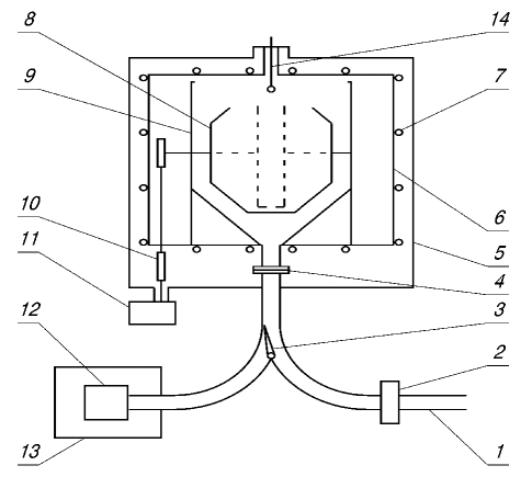
Figure 1: Schematic of the gravitational UCN storage system: 1–input neutron guide for UCN; 2–inlet valve; 3–selector valve (shown in the position in which the trap is being filled with neutrons); 4–foil unit; 5–vacuum volume; 6–separate vacuum volume of the cryostat; 7–cooling system for the thermal shields; 8–UCN storage trap (the dashed lines depict a narrow cylindrical trap); 9–cryostat; 10–trap rotation drive; 11–step motor; 12–UCN detector; 13–detector shield, and 14–vaporizer.

The neutron lifetime was measured by the so-called size extrapolation method. To this end, two UCN traps with different dimensions were employed. The first trap was quasi-spherical, consisting of a horizontal cylinder of 26 cm in length and 84 cm in diameter that was “crowned” by two 22-cm-high truncated cones with a smaller diameter of 42 cm. The second trap was cylindrical, with the length of 14 cm and 76 cm in diameter. The frequency of neutron collisions with the walls of the second trap was approximately 2.5 times higher than that in the first trap. In Fig. 1, the narrow cylindrical trap is depicted by dashed lines.

A typical measurement of the counting rate at the detector in a data cycle with a narrow trap is shown in Fig. 2. Figure 3 shows a similar measurement for data cycle taken with a quasispherical trap.

Figure 2: Time diagrams of the storage cycle for two different holding times in a narrow trap. 1–filling, 160 s (time of trap rotation (35 s) to monitoring position is included); 2–monitoring, 300 s; 3–holding, 300 s or 2000 s (time of trap rotation (7 s) to holding position is included); 4–emptying, with five periods of 150, 100, 100, 100, and 150 s (with time of trap rotation 2.3, 2.3, 2.3, 3.5, and 24.5 s to each position included); 5–measurement of background, 100 s.

Figure 3: Time diagrams of the storage cycle for two different holding times in a quasispherical trap. 1–filling, 160 s (time of trap rotation (35 s) to monitoring position is included); 2–monitoring, 300 s; 3–holding, 300 s or 2000 s (time of trap rotation (7 s) to holding position is included); 4–emptying, with five periods of 150, 100, 100, 100, and 150 s (with time of trap rotation 2.3, 2.3, 2.3, 3.5, and 24.5 s to each position included); 5–measurement of background, 100 s.

At the beginning of a measurement cycle, the trap is in the “window-down” position, as it is being filled with UCN. After this, the trap is rotated into the monitoring position $\theta=30^{\circ}$, in which the trap window height is approximately 10 cm lower than in the “window-up” position. The filling process can be monitored by the UCN detector (see Fig. 1) through a slit in the selector valve. After the trap has been rotated into the monitoring position, the selector valve is switched into the position in which UCN are registered. The trap is maintained in the monitoring position for 300 s. The neutrons that are in volume between the trap walls and the cryostat walls are registered by the detector. During this period, neutrons with energies higher than the gravitational barrier leave the trap (see Fig. 2). The trap is rotated into the “window-up” position after the monitoring period. The procedure of the neutron filling and preparation of the UCN spectrum takes about 700 s; in the left axis of Fig. 2 the counting rate is presented on a logarithmic scale: the counting rate for the subsequent procedures (700–3000 s) are presented with a greater detail on a linear scale (the right axis of Fig. 2). After a short (upper half of Fig. 2) or long (lower part of Fig. 2) storage time, the trap is rotated in steps through five positions, and in each of these positions it is kept fixed for 100–150 s, so that the UCN can be registered. The neutrons detected after the each rotation have different mean energies. After all the UCN have left the trap, the background count rate is measured.

The angular positions of the quasispherical trap window and the mean values of the UCN energies in each discharge are given by
$\theta=30^{\circ}$ (monitoring position);
$\theta=40^{\circ},E_{UCN}=62.3$ neV;
$\theta=50^{\circ},E_{UCN}=56.4$ neV;
$\theta=55^{\circ},E_{UCN}=52.3$ neV;
$\theta=70^{\circ},E_{UCN}=43.2$ neV;
$\theta=180^{\circ},E_{UCN}=26.7$ neV.

The angles are given with respect to the vertical up direction and were chosen in such a way that there will be an equal fraction of the spectrum emptied at each position (Unfortunately, the third portion was not successfully optimized, which is clearly obvious from Fig. 2.) The diameter of the narrow trap is smaller compared to the quasispherical trap. Therefore, slightly different angles for a narrow trap were chosen to obtain the same energy intervals.

III Methods of extrapolation to the neutron lifetime

III.1 Basic relations

The storage time for UCN in a system with a loss vessel is given by:

$$\tau_{st}^{-1}=\tau_{n}^{-1}+\tau_{loss}^{-1}$$ (5)

Here, the total UCN loss $\tau_{st}^{-1}$ comprises two terms, namely, the probability of neutron $\beta$ decay $\tau_{n}^{-1}$, and the probability $\tau_{loss}^{-1}$ of UCN losses. The success of the experiment is related to the fact that $\tau_{loss}^{-1}$ is small compared to $\tau_{n}^{-1}$. In our experiment, $\tau_{loss}^{-1}$ is 1% from $\tau_{n}^{-1}$. Therefore the measurement of $\tau_{loss}^{-1}$ with 10% accuracy gives the opportunity of $\tau_{n}^{-1}$ determination with the 0.1% or $\pm 0.8$ s accuracy.

Although the task of calculating $\tau_{loss}^{-1}$ with 10% accuracy looks rather simple, it should be done very carefully. Therefore, we will consider all stages of the $\tau_{loss}^{-1}$ calculation in succession and in detail.

Let us imagine monoenergetic UCN captured in a trap with volume $V$ and surface area $S$. For simplicity, we will neglect gravity for the moment. The total number of UCN in the trap will be

$$N(E)=V\cdot\rho(E),$$ (6)

where $\rho(E)$ is the UCN number density, which depends on the UCN energy $E$. The number of UCN lost in the trap per second will be

$$\frac{dN(E)}{dt}=\left({1\mathord{\left/{\vphantom{14}}\right.\kern-1.2pt}4}\right)v(E)\rho(E)S\mu(E),$$ (7)

where $v(E)$ is the UCN velocity and the function $\mu(E)$ gives the UCN losses from reflection, which depends on the UCN energy and on some properties of the trap walls. (Note that $\frac{1}{4}v\rho S$ is the flux of UCN on the trap surface.) Using Eqs. (6) and (7) one can write the expression for loss probability on the trap walls as

$$\tau_{loss}^{-1}(E)=\frac{dN(E)}{N(E)dt}=\frac{\left({1\mathord{\left/{\vphantom{14}}\right.\kern-1.2pt}4}\right)v(E)\rho\mbox{(}E\mbox{)}S\mu(E)}{V\cdot\rho\mbox{(}E\mbox{)}}$$ (8)

or

$$\tau_{loss}^{-1}(E)=\frac{S}{4V}\cdot v(E)\cdot\mu(E)$$ (9)

If we define $l$ as a mean free path of UCN in the trap ($l={4\cdot V}\mathord{\left/{\vphantom{{4\cdot V}S}}\right.\kern-1.2pt}S$) and $f(E)$ as the UCN collision frequency ($f(E)=v(E)/l$), Eq. (9) for the loss probability can be simplified to

$$\tau_{loss}^{-1}=f\left(E\right)\cdot\mu\left(E\right).$$

By assuming that the UCN are reflected from a potential step with real (U${}_{0})$ and imaginary (W) parts, the UCN losses from reflection can be represented in the following well-known form Ign90 :

$$\mu(y)=\frac{2\eta}{y^{2}}\cdot(\arcsin y-y\sqrt{1-y^{2}})\approx\left\{{{\begin{array}[]{*{20}c}{\pi\eta,y\to 1\hfill}\\ {\frac{4}{3}\eta y,y<<1\hfill}\\ \end{array}}}\right.$$ (10)

where $\eta=W/U_{0}=b^{\prime}/b$ is the loss factor determined by the ratio of the imaginary to real parts of the potential or the scattering amplitudes, and $y=(E/U_{0})^{1\mathord{\left/{\vphantom{12}}\right.\kern-1.2pt}2}$.

In Eq.(10), the energy UCN loss function has been averaged over the isotropic distribution of the incidence angles. Using the optical theorem, we can write the imaginary part of the scattering amplitude in the following form Ign90 :

$$b^{\prime}=\frac{{\sigma_{abs}+\sigma_{upscat}(T)}}{{2\lambda}}$$

The capture and inelastic-scattering cross sections are proportional to the neutron wavelength $\lambda$, with the result that neither $b^{\prime}$ nor $\eta$ depends $\lambda$ or the neutron energy $E$. However, the loss factor is temperature dependent, $\eta=\eta(T)$, owing to the temperature dependence of the inelastic-scattering cross section $\sigma_{upscat}(T)$.

It looks very useful to rewrite the right-hand side of Eq.(9) as the product of two factors, one depending only on the trap temperature and the other only on the UCN energy:

$$\tau_{loss}^{-1}(T,E)=\eta(T)\cdot\gamma(E)$$ (11)

where $\gamma(E)$ is the normalized loss rate which depends on the UCN energy and the trap dimensions.

Taking into account Eq.(11) we can rewrite Eq.(5) as

$$\tau_{st}^{-1}(E)=\tau_{n}^{-1}+\eta(T)\cdot\gamma(E)$$ (12)

Now we are ready to explain the principle of how to extract the neutron lifetime value from the experimental storage times. For this purpose, we have to measure the UCN storage time in two experiments ($\tau_{1}$ and $\tau_{2}$). The normalized loss rates $\gamma_{1}$ and $\gamma_{2}$ should be different in these measurements. Using Eq.(12) for the total UCN loss probability, namely,

$$\tau_{1}^{-1}=\tau_{n}^{-1}+\eta\gamma_{1}(E)$$ (13)

$$\tau_{2}^{-1}=\tau_{n}^{-1}+\eta\gamma_{2}(E)$$ (14)

we find that

$$\tau_{n}^{-1}=\tau_{1}^{-1}-\frac{{\tau_{2}^{-1}-\tau_{1}^{-1}}}{{{{\gamma_{2}(E)}\mathord{\left/{\vphantom{{\gamma_{2}}{\gamma_{1}-1}}}\right.\kern-1.2pt}{\gamma_{1}(E)-1}}}}$$ (15)

One can see that Eq.(15) contains only the ratio of the normalized loss rates $\gamma_{1}$ and $\gamma_{2}$. Different values of the UCN normalized loss rate $\gamma$ can be obtained by using traps of different dimensions and/or different values of the UCN energy. Therefore, we can use either energy extrapolation or size extrapolation.

For the energy extrapolation we will use one trap and will capture the UCN of different energy. Using Eqs.(13) and (14) we can extrapolate to zero losses to obtain $\tau_{n}^{-1}$. But the rest of the dependence of $\tau_{n}^{-1}$ on the function $\mu(E)$ exhibits some problem. Actually the real function $\mu(E)$ may differ somewhat from that of the adopted form (10), which was calculated for the ideal potential step.

To exclude the effect of the energy dependence $\mu(E)$ on the result, we can extrapolate to zero losses by using data on the storage of UCN with the same mean energy in traps of different dimensions. This method is called the size extrapolation method. In this case the ratio of the normalized loss rate $\gamma_{2}$ to $\gamma_{1}$ depends only on the trap sizes:

$${\gamma_{2}}\mathord{\left/{\vphantom{{\gamma_{2}}{\gamma_{1}}}}\right.\kern-1.2pt}{\gamma_{1}}={\frac{S_{2}}{V_{2}}}\mathord{\left/{\vphantom{{\frac{S_{2}}{V_{2}}}{\frac{S_{1}}{V_{1}}}}}\right.\kern-1.2pt}{\frac{S_{1}}{V_{1}}}$$ (16)

Thus, the effect of any energy dependence is excluded entirely. Clearly, this is valid only in the absence of gravity.

In a gravitational field UCN kinetic energy ${E}^{\prime}$ becomes dependent on the height: ${E}^{\prime}=E-mgh$, where $h$ is the height measured from the bottom of the trap and $E$ is the UCN energy at $h=0$. So the gravity-free equation (8) has to be modified. We have to replace $E$ by $E-mgh$ and to integrate with respect to $h$ on the trap surface in the numerator and on the trap volume in the denominator:

$$\tau_{loss}^{-1}(E)=\eta\cdot\gamma\left(E\right)=$$

$$\frac{\int\limits_{0}^{E\mathord{\left/{\vphantom{E{mg}}}\right.\kern-1.2pt}{mg}}{\mu(E-{h}^{\prime})\cdot v(E-{h}^{\prime})\cdot\rho(E-{h}^{\prime})dS(h)}}{4\int\limits_{0}^{E\mathord{\left/{\vphantom{E{mg}}}\right.\kern-1.2pt}{mg}}{\rho(E-{h}^{\prime})dV(h)}},$$ (17)

where ${h}^{\prime}=mgh$. The UCN number density is proportional to $\sqrt{{\left({E-mgh}\right)}\mathord{\left/{\vphantom{{\left({E-mgh}\right)}E}}\right.\kern-1.2pt}E}$,

In reality, when gravity is present, complete exclusion of $\mu(E)$ is impossible because of the integral nature of Eq.(III.1). However, the residual effect of the dependence $\mu(E)$ on the neutron lifetime is negligible. It will be shown further that in our experiment on the neutron lifetime measurement, the contribution from uncertainty of this dependence does not exceed 0.144 s, whereas the statistical accuracy of the measurement was 0.7 s. To demonstrate this fact the UCN normalized loss rates $\gamma$ were calculated for a series of model dependencies $\mu(v)$:

1. $\mu(v)\sim$ constant,

2. $\mu(v)\sim v/v_{lim}$,

3. $\mu(v)\sim\left(v/v_{lim}\right)^{2}$,

4. $\mu(v)\sim\left(v/v_{lim}\right)^{3}$,
where $v_{lim}$ is the trap boundary velocity. A coefficient in these dependencies is not important because it is outside the integral in Eq.(III.1) and is canceled in Eq.(15). Then, the values of the neutron lifetime were obtained by the size extrapolation method for each corresponding model dependency $\mu_{i}(v)$. The differences between the neutron lifetime values for $\mu(v)$ from Eq.(10) and for the model dependencies $\mu_{i}(v)$ are as follows:

1. $-0.158$ s,

2. $-0.022$ s,

3. $+0.1$ s, and

4. $+0.217$ s.
The linear dependence $v/v_{lim}$ is the most similar to the theoretical dependence $\mu(v)$, especially for small velocities. The mean square value of the numbers listed is $0.144$ s and can be used as an estimation of the uncertainty of the neutron lifetime value owing to the uncertainty of the $\mu(v)$ function shape (see Table 1). In spite of the fact that the model dependencies $\mu_{i}(v)$ are very different, their influence on the result of the extrapolation to the neutron lifetime is rather weak. Therefore, the size extrapolation method based on the idea of using two traps makes it possible to reduce substantially systematic errors that are caused by the uncertainty of our knowledge about the function $\mu(E)$.

The effect from uncertainty of the dependence $\mu(E)$ on the neutron lifetime was also studied for the case of the energy extrapolation method. The differences between the neutron lifetime values for $\mu(v)$ from Eq.(10) and for the model dependencies $\mu_{i}(v)$ are as follows:

1. $-0.83$ s,

2. $0.76$ s,

3. $-1.93$ s, and

4. $-2.73$ s.
As expected, the dependence of the result of the energy extrapolation method on the $\mu(v)$ function shape is rather strong, going mainly to systematically low value of neutron lifetime. Therefore, we used the result of the size extrapolation as the final value of the neutron lifetime.

If we have more than two measurements, the neutron lifetime can be obtained by a linear regression of Eq.(12) with $\tau_{n}^{-1}$ and $\eta$ as free parameters. The UCN loss factor $\eta$ proves to be equal to the tangent of the slope angle of the extrapolation line. The UCN normalized loss rate $\gamma(E)$ with the trap walls can be computed according to Eq. (III.1). The results of calculation of the normalized loss rate are presented in Fig. 4.

The UCN storage time $\tau_{st}^{-1}$ can be calculated if we know the measured number of neutrons that remain in the trap after two different storage times:

$$\tau_{st}=\frac{{t_{2}-t_{1}}}{{\ln({{N_{1}}\mathord{\left/{\vphantom{{N_{1}}{N_{2})}}}\right.\kern-1.2pt}{N_{2})}}}},$$ (18)

where $N_{1}$ and $N_{2}$ are the numbers of neutrons left in the trap after storage times $t_{1}$ and $t_{2}$, respectively. There is no need to know the efficiency of the UCN detector, the probability of UCN losses as the neutrons travel along the neutron guide, and so forth, since Eq.(18) uses only the ratio of the numbers of neutrons.

Figure 4: The UCN normalized loss rate as a function of UCN energy for narrow cylindrical and wide quasispherical traps.

III.2 Calculation of normalized loss rate for the broad UCN spectrum in the trap

Previously it was demonstrated how one can calculate the normalized loss rate $\gamma(E)$ and fulfill the size extrapolation to the neutron lifetime for a the monoenergetic UCN spectrum. But in practice we have dealt with a rather broad spectrum.

To calculate the normalized loss rate for a broad UCN spectrum one has to integrate the Eq.(III.1) over the real spectral distribution of UCN in the trap. Hence the task of calculating the normalized loss rate for a broad spectrum leads to the task of spectrum measurement.

There are two ways to determine the UCN spectrum in the trap: 1. by direct measurement of the differential UCN spectrum by means of the step-by-step rotation of the UCN trap as was previously described and 2. by measuring the integral UCN spectrum and then calculating its differential form. In the first case, each portion of the spectrum will be measured in a different time. Therefore, it is necessary to introduce a correction for the UCN decay and losses. In the second case, introduction of this correction is not required. We used the second way, measuring the number of neutrons in the trap by means of the trap rotation to the down position from the different monitoring positions.

The differential spectrum of UCN captured into the trap, $N(E)$, can be calculated by the so-called integral spectrum $N_{int}(E_{up})$. The integral spectra for each trap were measured during a special experiment and the results are presented in Fig. 5.

The differential spectrum was taken as

$$N(E)=\rho_{0}\cdot\rho(E)\cdot V(E)\cdot\exp(-\alpha E),$$ (19)

where $\rho_{0}$ is the UCN density in phase space, $V(E)$ is the effective volume for UCN with energy $E$ in gravitational field, $E$ is the UCN energy at the trap bottom, $\alpha$ is the deformation parameter of the Maxwell spectrum, and $\rho(E)$ is Maxwell spectrum of UCN ($v^{2}dv\sim\sqrt{E}dE)$.

The function $V(E)$ depends on the trap configuration and was calculated from

$$V(E)=\int\limits_{0}^{E\mathord{\left/{\vphantom{E{mg}}}\right.\kern-1.2pt}{mg}}{\sqrt{\frac{E-mgh}{E}}}\cdot A(h)dh,$$ (20)

where $A(h)$ is the cross-sectional area of the trap at height $h$. The experimental values of integral spectra for each trap were fitted by the least squares method with a function that equals the integral from $N(E)$ [Eq.19]:

$$N_{int}(E_{up})=\rho_{0}\int\limits_{0}^{E_{up}}{V(E)\cdot\sqrt{E}\cdot}\exp(-\alpha E)dE.$$ (21)

The values of parameters $\alpha$ and $\rho_{0}$ were determined as a result of the least squares fitting, which is shown in Fig. 5 by a solid line. The differential spectra of UCN captured in the trap were calculated according to Eq.(19) and are presented in Fig. 6 for quasispherical and cylindrical traps. The shape of the spectra depends mainly on the parameter $\alpha$. One can determine the differential spectrum by a simple differentiation of the measured integral spectrum. This method looks more straightforward, as it does not need any model function such as Eq.(19), but direct differentiation introduces some additional uncertainties. Finally, both methods result in approximately the same UCN spectrum uncertainty in Table 1.

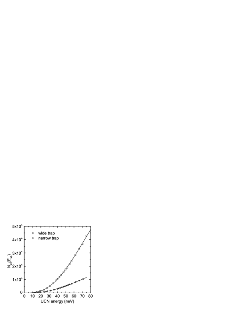
Figure 5: The integral UCN spectra. The open squares represent the results of measurements for a quasispherical trap, and the open circles are the results of measurements for a cylindrical trap. The results of the least squares fitting are shown by solid line.

The main procedure of the storage time measurement uses five successive emptying stages, as shown in Figs. 2 and 3. Let us discuss now the method of the spectrum calculation for each successive emptying. Each emptying differs by the height of the gravitational barrier for UCN, which is defined by the height of the low edge of the trap window relative to the trap bottom. The neutrons with energies higher than this gravitational barrier can leave the trap. Suppose for the moment that all such neutrons leave the trap. This is strictly valid if emptying times are infinitely long. In this case, the spectrum of captured UCN should be divided into intervals of UCN energy, as shown in Fig. 6 by vertical lines. The position of each line is defined by the height of the gravitational barrier for the corresponding emptying.

Figure 6: The differential UCN spectra in quasispherical and cylindrical traps. The position of each vertical line is defined by the height of the gravitational barrier for corresponding emptying.

The values of the normalized loss rate $\gamma_{i}$ for energy interval $i$ can be calculated as follows:

$$\bar{\gamma}_{i}=\frac{\int_{E_{i-1}}^{E_{i}}{\gamma(E)\cdot N(E)dE}}{\int_{E_{i-1}}^{E_{i}}{N(E)dE}},$$ (22)

where $E_{i}$ is the bound of energy interval $i$, with $E_{0}=0$.

However, in reality the emptying times are finite. Hence some neutrons with energies greater than the gravitational barrier do not leave the trap. The spectrum calculation should take into account five successive emptyings with finite time and the rotation of the trap with finite speed. The best method for such a calculation is a Monte Carlo simulation. The results of such a Monte Carlo simulation for narrow cylindrical and quasispherical traps are presented in Fig. 7. Compared to the spectra for the interval method (see Fig. 6) one can observe the shape change and shift of mean energies to the high end.

Figure 7: Monte Carlo simulation of UCN differential spectra in a cylindrical trap (solid line) and in a quasispherical trap (dotted line) for each of five emptyings. Spectra are normalized to unity. The probability of UCN diffuse scattering used in the simulation is 10%.

The normalized loss rate $\gamma_{i}$ for the $i$-emptying can be calculated according to

$$\bar{\gamma}_{i}=\frac{\int_{0}^{\infty}{\gamma(E)\cdot N_{i}(E)dE}}{\int_{0}^{\infty}{N_{i}(E)dE}},$$ (23)

where $N_{i}(E),i=1\ldots 5$, is the UCN spectrum of the $i$-emptying as shown in Fig. 7.

A comparative analysis of the extrapolation of the experimental data to the neutron lifetime using Eqs.(22) and (23) shows that the difference in the extrapolated value $\tau_{n}$ is only $0.15$ s.

This method of calculating $\gamma_{i}$ on energy intervals was used during the experimental data treatment, but the energies $E_{i}$ and $E_{i-1}$ in Eq.(22) were corrected for incomplete emptying. So, the effect of the mean energy shift was taken into account. Note that this shift of the mean energy is slightly different for cylindrical and quasispherical traps because of the different ratio of the window area to the trap volume for these traps. One can observe this effect in Fig. 7. However, the influence of this effect is rather small. To check it, we used the same spectrum for the calculation of $\gamma$ values in cylindrical and quasispherical traps. The extrapolated value of the neutron lifetime was shifted by 0.23 s compared to the extrapolation where we used the native spectra for different traps.

IV Neutron lifetime measurements

IV.1 Low-temperature perfluoropolyether

For this experiment, a new type of material – a low-temperature, fully fluorinated polymer – was proposed Pok99 and used for coating trap walls. The chemical formula of the substance – perfluoropolyether (PFPE) – is $CF_{3}O(CF_{2}O)_{n}(CF_{2}CF_{2}O)_{m}(OCF_{2}CF_{2}O)_{l}CF_{3}$ with $n\approx 30.3$, $m\approx 1.5$, $l\approx 0.2$, and molecular weight M=2350; its vapor pressure at room temperature was measured to be about $1.5\times 10^{-3}$ mbar and the pour temperature was measured to be about $-100^{\circ}$C Pok03 . This substance was deposited on the trap surface by evaporation in vacuum.

The PFPE contains only C, O, and F, so its neutron-capture cross section is small. As a result of a preliminary study of several types of PFPE, it was found Ste02 that the quasielastic and inelastic UCN scattering in PFPE for $T<-120^{\circ}$C is much weaker than in ordinary Fomblin at room temperature. Quasielastic UCN scattering is completely suppressed for $T<-120^{\circ}$C Ste02 , and because of the neutron inelastic scattering the expected UCN loss factor $\eta$ amounts to roughly $2\times 10^{-6}$ Pok03 .

Before the beginning of the PFPE deposition procedure, a spherical vaporizer with tiny holes was heated to 140^∘C with an electric heater. Then gaseous helium was utilized to force three cubic centimeters of liquid into the vaporizer’s chamber along a vertical tube. The deposition of the PFPE was done by evaporation with the evaporated substance from the vaporizer being settled and frozen onto the inner walls of the trap cooled to $-150^{\circ}$C. To achieve homogeneity, the vaporizer was moved up and down.

IV.2 Study of the coating properties of PFPE

To check the quality of the PFPE film, a copper trap with a titanium coating was employed. Titanium has a negative scattering length and does not generate a reflecting potential for UCN. Ultracold neutrons cannot be stored in such a trap if the titanium coating is not covered with a layer of PFPE. The trap was a 50-cm-long cylinder with a diameter of 76 cm. A stable storage time $\tau_{st}=869.0\pm$0.5 s was achieved after several depositions of PFPE (with a total thickness of 15 $\mu$m) with the temperature of the trap walls varying from $-140^{\circ}$ to $-150^{\circ}$C and after a single heating-cooling cycle in which the trap temperature was first raised to room temperature and then brought down to T = $-160^{\circ}$C. The repetition of the thermal cycling had no effect on the UCN storage time in the trap. It is quite possible that at room temperature the PFPE filled all the gaps and cracks in the trap walls and formed a perfect surface. In addition, PFPE was degassed in the thin layer at room temperature. Such a coating is extremely stable, and no essential variation in the storage time was detected during the eight-day period of observation. Subsequent depositions had no effect on the value of the UCN storage time in the trap.

The traps used in the final measurements (a quasispherical trap and a narrow cylindrical one) were coated with beryllium. Since beryllium constitutes a good reflector of ultracold neutrons, the trap walls can be cooled to even lower temperatures, since the appearance of any microcracks in the coating has a small influence on the UCN lifetime in the trap. Using a beryllium-coated trap, we studied the temperature dependence of the storage time for a quasispherical trap coated with PFPE [Fig. 8(a)].

PFPE was frozen on the trap wall at T = $-155^{\circ}$C, then the trap was slowly heated to T = $-50^{\circ}$C, and finally cooled down again to T = $-160^{\circ}$C. In this way, we covered up the layer defects with oil when it was fairly liquid. After this temperature cycling was completed, the measured storage time turned out to be longer, 872.2$\pm$0.3 s, than immediately after sputtering, 850$\pm$1.8 s. Repeated warming and cooling cycles did not change the UCN storage time of the traps (see Fig. 11).

This procedure (heating after evaporation at T = $-160^{\circ}$C) is extremely important because the oil in a liquid form coats all surface defects because of the effect of the surface tension of PFPE.

By comparing the storage time of the trap with a titanium substrate and with a beryllium substrate we can estimate the part uncoated by the PFPE surface. Bearing in mind that the titanium and beryllium traps differ in dimensions, we calculated the difference between the expected and measured storage times for the titanium trap, which was 1.9$\pm$0.6 s. This is equivalent to an uncovered part of the surface area of the titanium trap equal only to ($4.4\pm 1.3)\times 10^{-7}$. Hence, the reproducible PFPE coating can be obtained irrespective of the material and shape of the trap. For this reason, there is no need to examine the different loss factors $\eta$ for various traps with a beryllium sublayer under a PFPE coating.

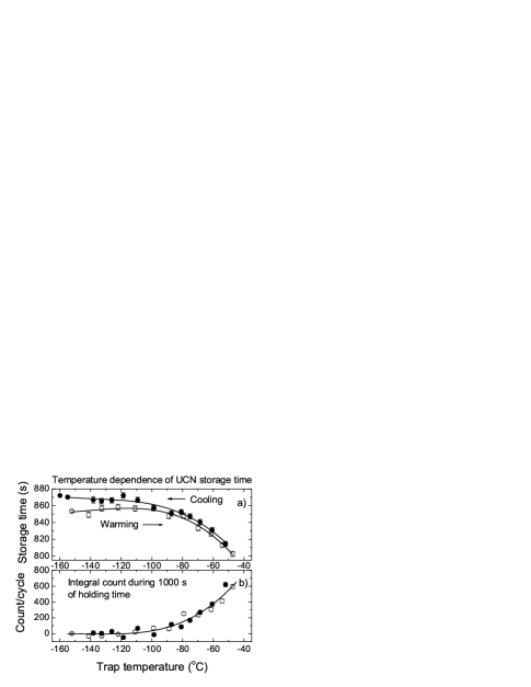
Figure 8: Temperature dependence of (a) the UCN storage time in the course of warming (empty circles) and the cooling again (full circles) after the first evaporation of PFPE at T = –155^∘C and (b) the integral count for a 1000-s storage period after subtraction of background and count rate of UCN that have energy higher than the gravitational barrier (see Fig. 10 and Sec. IV.6)

.

IV.3 Study of quasielastic UCN scattering

In the course of investigations that used a beryllium-coated trap, the quasielastic UCN scattering by PFPE was studied.

In our installation, the principle of the gravitational valve was used. A gravitational valve cannot store UCN with energy more than the gravitational barrier. If UCN during the storage take up additional energy they will leave the trap and reach the detector.

Figure 8(b) shows the number of ultracold neutrons that leave the trap during a 1000-s (761-1760 s) storage period as a function of the trap temperature. Here the background and count rate of UCN that have energy higher than the gravitational barrier are already subtracted (see Fig. 10 and Sec. IV.6). In the process, we observed an additional counting rate (on top of the background noise), which fell off exponentially with the passage of the time of UCN storage in the trap. The additional counting rate appears because the UCN acquire energy in their quasielastic scattering by PFPE. These neutrons leave the trap, which drives the counting rate at the detector upward. The counting of quasielastically scattered UCN becomes indistinguishable against the background (i.e., it disappears) as T $<-120^{\circ}$C. This result is in qualitative agreement with that of measuring the quasielastic UCN scattering by PFPE studied in our previous work Ste02 .

Here, this process was studied in more detail, particularly at temperature T = $-160^{\circ}$C. At T =$-60^{\circ}$C we find reasonable agreement with the result of our previous work Ste02 . The illustration of the process of UCN upscattering at T = $-60^{\circ}$C is shown in Fig. 9. We can see the clear definite exponent with the UCN storage time in the trap.

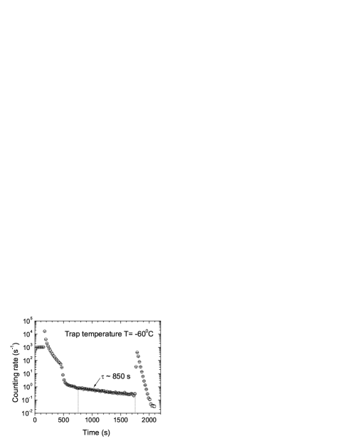
Figure 9: Time diagram of the neutron storage cycle in a quasispherical trap at T = $-60^{\circ}$C. The exponential time of emptying of quasielastically scattered UCN is defined by the UCN storage time in the trap.

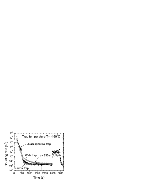
Figure 10: Time diagram of the neutron storage cycle in narrow cylindrical, wide cylindrical, and quasispherical trap at T = $-160^{\circ}$C. The exponential time of emptying of UCN that have energy higher than the gravitational barrier depends on the shape of the trap (see Sec. IV.6). For the quasispherical trap the exponential time of emptying of UCN that have energy higher than the gravitational barrier is $\sim 230$ s. The time diagram during a storage period has no dependence on exponential times such as the storage time in the trap ($\sim 800-850$ s), because the process of quasielastic UCN scattering is suppressed at T = $-160^{\circ}$C.

The most important studies have been carried out at a trap temperature T = $-160^{\circ}$C. Figure 10 shows the counting rate of the detector during UCN storage in the traps with T = $-160^{\circ}$C. Just after the trap rotation in the storage position (hole up) we can see the counting rate of UCN whose energy is above the gravitational barrier. The exponential time is different for different traps (narrow, wide cylindrical, and quasispherical) because of the different ratio of the window area to the trap volume. The exponential time of counting rate is in a reasonable agreement with Monte Carlo calculations. For the narrow trap this process is the fastest (about 30 s); therefore this curve is the most preferable for the analysis of UCN upscattering.

The counting rate of quasielastically scattered UCN should be proportional to the number of UCN in the trap, UCN collision frequency with the trap walls, and probability of UCN upscattering. The analysis shows that the counting rate during a storage period contains no counts with an exponential time like the storage time (about 800–850 s). But this conclusion is valid with finite uncertainty. Therefore, we can only calculate the upper limit for the probability of UCN upscattering with energy transfer about 20 neV. This upper limit is $6\times 10^{-9}$ per collision. From this upper limit of UCN probability of leakage at storage in the trap we can also infer the upper limit of the correction to the neutron lifetime, which is less than 0.03 s. It should be mentioned that the estimation is valid for any process of low-energy transfer owing to the interaction with the trap surface as well as the interaction inside the trap volume.

Thus, it turned out that for T $<-120^{\circ}$C, the quasielastic UCN scattering can be ignored. Our measurements were made at T = $-160^{\circ}$C to guarantee that quasielastic scattering does not affect the results.

The effect of emptying UCN that have energy higher than the gravitational barrier for the quasispherical trap is insignificant too. That part of UCN that have energy higher than the gravitational barrier is $10^{-3}$ (i.e., on the level of statistical error). Moreover, our data were corrected for this effect.

IV.4 Study of the stability and reproducibility of coating

The stability and integrity of the coatings on various traps constitute the most important conditions for the use of the size extrapolation method in measuring the neutron lifetime. Therefore, the quality of the PFPE coating was checked many times during measurements. Figure 11 gives eight results of the measurements of the neutron storage time for a quasispherical trap and seven analogous results for a narrow trap. The measurements were carried out after new depositions, heating, and cooling with a subsequent new deposition, etc. After a liquid-helium cryogenic pump was mounted near the storage volume, the trap’s vacuum was improved from $5\times 10^{-6}$ to $3\times 10^{-7}$ mbar. The storage time during the experiment on the measurement of the neutron lifetime agrees, within approximately one second, for the wide trap and, within marginally broader limits, for the narrow trap. This proves that the PFPE coatings are stable and reproducible for various traps.

Figure 11: Demonstration of the stability of a PFPE coating during measurements. The UCN storage times for the wide and narrow traps differ because of the different frequencies of UCN collisions with the trap walls.

Thus, assuming that the substances used for coatings in various UCN traps were identical and taking into account the exceptionally high coating properties of a Fomblin oil (owing to its surface tension) and the absence of coating degradation, we believe that the same loss factor $\eta$ can be used for different traps.

The level of statistical accuracy of our experiment agrees with the requirement that the loss factor $\eta$ within about 5% is the same for different traps. However, test experiments with the titanium trap have convinced us that this requirement is met with a much higher accuracy, because any defects of coating of the titanium trap would cause the UCN storage times to be very unstable.

The reasons for using the same loss factor $\eta$ for different traps are the following:

• The coating of the traps was made of the same substance; moreover, the substance was taken from the same bottle.

• There is a high coating capacity of the oil in liquid form owing to the effect of the surface tension of PFPE.

• There is an absence of degradation of coating properties during the test experiment with the Ti trap.

• The experiment with a Ti trap proves that the part of the trap surface uncoated by PFPE is negligible small ($4.4\times 10^{-7}$).

• Some flaking of PFPE coating in time would be discovered immediately during the test experiment with the Ti trap.

Thus, according to the result of the test experiment with the Ti trap, we have reasons to consider that the stability and repeatability of the PFPE coating offer a much higher level of precision than the statistical accuracy of measurements with a Be trap.

IV.5 Measurement data and extrapolation to the neutron lifetime

Figure 12 presents the results of measurements of the UCN storage times for various energy intervals and different traps (wide and narrow) as a function of the normalized loss rate $\gamma$. The UCN storage time was calculated according to Eq.(18). The values of $N_{1}$ and $N_{2}$ were corrected for the background, which was measured at the end of each data-acquisition cycle. The value of $N_{1}$ of the first emptying angle for the quasispherical trap was corrected for the effect of UCN that have an energy higher than the gravitational barrier. This correction is about 3.5 standard deviations ($3.5\sigma$) of this point. There are no other corrections for $N_{1}$ and $N_{2}$. Corrections to the $\gamma$ function were discussed in Sec. III.2.

Extrapolation of all the data to the neutron lifetime yields a value of 877.60$\pm$0.65 s at $\chi^{2}$= 0.95, which means that a combined extrapolation is possible. However, if we build an energy extrapolation for each trap and combine the two results, we get 875.55$\pm$1.6 s.

To use the size extrapolation method, we have to combine the values obtained from different traps within the same UCN energy range and then calculate the average value of all the resultant values of the neutron lifetime.

Figure 13 demonstrates the results of size extrapolation to the neutron lifetime for different energy ranges. The average value of the neutron lifetime obtained by the size extrapolation method was 878.07$\pm$0.73 s.

The results corresponding to these two methods differ by 1.5$\sigma$. The loss factor obtained in this experiment, $\eta=2\times 10^{-6}$, agrees with the value found in the transmission experiment Pok03 . For the final value of the neutron lifetime we prefer using the result of size extrapolation, which depends rather weakly on $\mu(E)$ and which we consider more reliable.

Figure 12: Result of extrapolation to the neutron lifetime when combined energy and size extrapolations are used. The open circles represent the results of measurements for a quasispherical trap, and the full circles the results of measurements for a cylindrical trap.

Figure 13: Extrapolated values of the neutron lifetime for different mean UCN energies, when size extrapolation is used. The solid, straight line corresponds to the average value of neutron lifetime for given measurements.

IV.6 Monte Carlo simulation of the experiment and systematic errors

To estimate the accuracy and test the reliability of the size extrapolation method in which the value of the function $\gamma$ must be calculated, we performed a simulation of the experiment using the Monte Carlo method.

The adopted Monte Carlo model describes the behavior of neutrons with allowance for a gravitational field, the shape of the storage traps, trap losses $\eta$ = 2$\times$10^-6, and the geometries of the secondary volume and of the ultracold neutron guide. The start spectrum for modeling is the spectrum measured in the experiment. The angular distribution was prepared by simulation of UCN storage in the trap for 50 s with 100% diffuse reflections without any losses before the start of the main simulation process. As a result, we were able to simulate directly the measurement procedure and build a time diagram for the counting rate at the detector, similar to the one shown in Fig. 2. The UCN storage time in the traps and the extrapolation to the neutron lifetime that rely on the computed function $\gamma$ were calculated in the same way as in the experiment. The single adjustable parameter in the Monte Carlo model was the coefficient of UCN diffuse scattering in the interaction with the trap surface. All the information about the probability of mirror reflection is extremely important. For instance, if it equals 99.9%, the behavior of UCN in the trap becomes strongly correlated and the resulting prediction becomes extremely difficult to make.

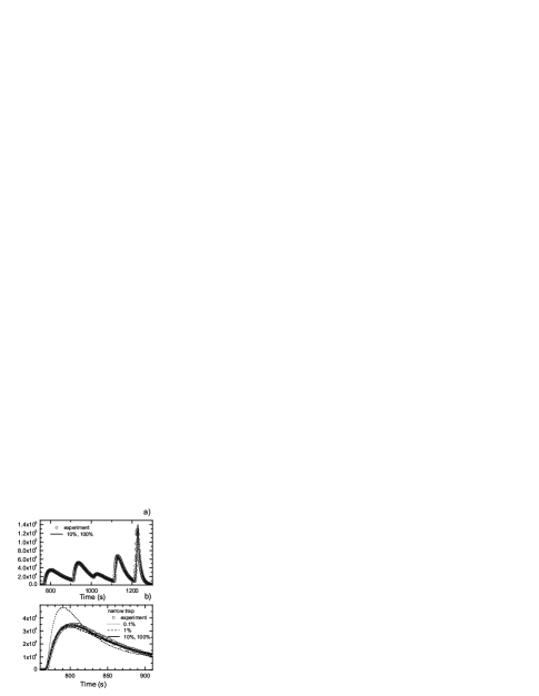
Figure 14: Simulation of an experiment by the Monte Carlo method, consisting in simulating the neutron discharge from a narrow cylindrical trap. The dotted curve corresponds to the results of calculations with a 0.1% diffuse reflection probability; the dashed curve corresponds to a 1% diffuse reflection probability, and the solid curve to 10% and 100%.

A comparison of the results of Monte Carlo calculations for different values of the diffuse scattering probability and the experimental results (Fig. 14) makes it possible to conclude that the probability of UCN diffuse scattering by the PFPE coating amounts to about 10%. In Fig. 14(a) we compare the experimental diagram and the Monte Carlo simulation diagram, obtained with the diffuse scattering coefficients equal to 10% and 100%. The experiment is successfully described for both diffusivity values. However, when the diffuse scattering probability is 0.1%, the agreement between the calculated and experimental results becomes unsatisfactory. The results of such calculations for the first part of the time diagram, which is the most sensitive to the neutron mirror reflection, are shown on a larger scale in Fig. 14(b).

The final simulation of the experiment was made for 10% and 1% diffuse reflection probabilities. The model storage times extrapolated to the neutron lifetime for the wide and narrow cylindrical traps and five different UCN energy ranges are presented in Fig. 15. To simplify the Monte Carlo calculations for the wide trap, we used cylindrical traps instead of quasispherical ones. In the final analysis of the data obtained with this model, we reproduced the value of the neutron lifetime adopted in the calculation with an accuracy of $\pm$0.236 s. This accuracy was limited by the statistical accuracy of the Monte Carlo calculations. About 10⁹ neutrons were used in the simulations presented in Fig. 15. This number corresponds to the beginning of the monitoring process. Thus, because we employed the computed value of the function $\gamma$, the systematic uncertainty of the size extrapolation method amounted to $\pm$0.236 s.

It should be mentioned that Monte Carlo simulations with a probability of diffusive scattering of 0.1% have also been carried out. Figure 16 demonstrates the result of this simulation. All points besides the first emptying show the shorter storage time because the cleaning of spectrum becomes less effective and neutrons leave the trap even during the storage period. The first emptying should be excluded because it is near the edge of the energy spectrum in the Monte Carlo calculations. This picture visibly disagrees with the experimental plot (see Fig. 12), leading us to conclude that high mirror reflection did not take place in the experiment.

Figure 15: Monte Carlo experiment with a 1% and 10% diffuse reflection probability involving simulation of an extrapolation to the neutron lifetime. The circles represent the results of simulation for a wide trap and triangles the results of simulation for a narrow cylindrical trap. The open and full figures correspond to 1% and 10% diffuse reflection probability respectively.

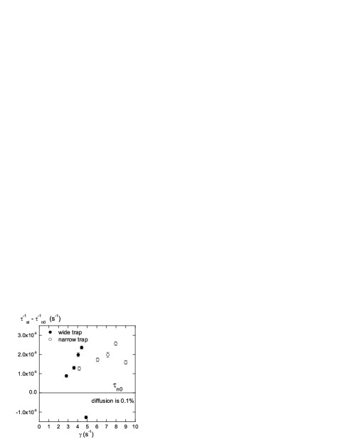
Figure 16: Monte Carlo experiment with a 0.1% diffuse reflection probability involving simulation of an extrapolation to the neutron lifetime. The full circles represent the results of simulation for a wide trap and the open circles the results of simulation for a narrow cylindrical trap.

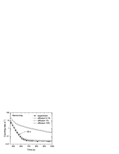
Figure 17: Monte Carlo simulation of leakage process of UCN exceeding the gravitational barrier of the trap from the narrow cylindrical trap. The results of Monte Carlo calculations with different diffuse reflection probability are presented: by up triangles with 0.1% diffusion, by squares with 1% diffusion and by down triangles with 10% diffusion. The filled circles represent the results of experiment.

Another piece of evidence for the absence of high mirror reflection comes from the analysis of the leakage process of UCN exceeding the gravitational barrier of the trap just after the beginning of storage process, which is shown in Fig. 17 for a narrow cylindrical trap and in Fig. 18 for a quasispherical trap. Monte Carlo simulation of this process shows that with high mirror reflection the tail of the time spectra of leaked neutrons has to be very long. The results of the experiment are consistent with the results of Monte Carlo simulation for diffuse reflection probability of more than 1%.

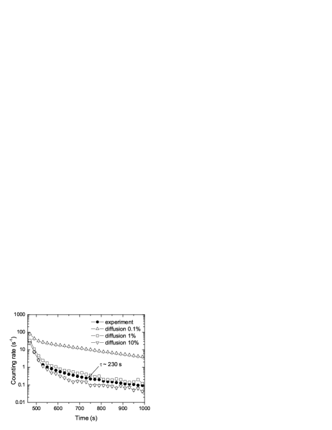
Figure 18: Monte Carlo simulation of leakage process of UCN exceeding the gravitational barrier of the trap from the quasispherical trap. The results of Monte Carlo calculations with different diffuse reflection probability are presented: by up triangles with 0.1% diffusion, by squares with 1% diffusion and by down triangles with 10% diffusion. The filled circles represent the results of experiment.

IV.7 Effect of residual gas on UCN storage

When the neutron lifetime is measured with a high precision, the effect of residual vacuum on the UCN loss cannot be ignored. For instance, a residual gas pressure of $5\times 10^{-6}$ mbar would introduce an error of about 0.4 s into the value of the UCN lifetime in the trap, which is comparable to the statistical accuracy of the measurements. Such a correction cannot be measured directly (e.g., by improving a vacuum pressure by an order of magnitude) because the expected effect is smaller than the statistical uncertainty.

The vacuum system of an installation is shown in Fig. 19. A “clean” vacuum volume is connected with turbo pump #1 by a pipe about 1.2 m of length and 90 mm in diameter. Turbo pump #1 has a pumping speed of about 550 l/s. Turbo pump #2 with a smaller pumping speed is connected to the output of the first turbo pump. A vacuum valve with a pneumatic drive allows separation of the main volume from the pumping system.

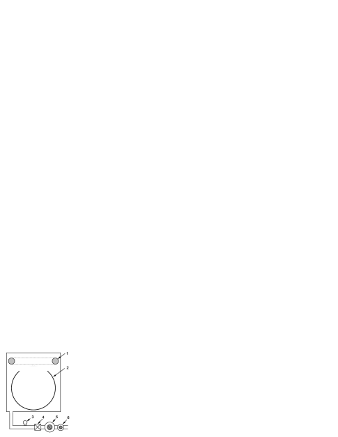
Figure 19: Vacuum system of “Gravitrap” installation: 1 - cryogenic vacuum pump; 2 - UCN trap; 3 - vacuum gauge; 4 - vacuum valve; 5 - turbo pump #1; 6 - turbo pump #2.

As one can learn from Fig. 19 the vacuum gauge is placed rather close to the turbo pump. There exists a pressure gradient in the vacuum pipe when the vacuum valve is open and turbo pump is on. In this situation, the vacuum gauge will detect some value of vacuum that can be far from the equilibrium value of vacuum for our system. Detecting the equilibrium value of vacuum requires some special actions. The vacuum valve was closed for some time. During several seconds the gradient of vacuum owing to the turbo pump disappears and we took the equilibrium value of vacuum from the vacuum gauge. All values of vacuum mentioned in the following were measured according to this simple procedure.

Of course, this procedure of measurement of equilibrium vacuum is valid only for a vacuum system without any temperature gradients. In our system, the main vacuum volume has a temperature of about –160^∘C, whereas the vacuum gauge is at room temperature. In this case, the “real” vacuum in the main vacuum volume ${P}^{\prime}$ will differ from the vacuum detected with the vacuum gauge, $P$, by a temperature-dependent factor $k$: ${P}^{\prime}=k(T_{1},T_{2})\cdot P$, where $T_{1}$ and $T_{2}$ are the temperatures of the main vacuum volume and vacuum pipe. The factor $k$ can be calculated with some precision, but it is important for us that this factor does not depend on the pressure, because we are going to extrapolate to zero vacuum using the measurements at the two different vacuums.

The main measurements of the UCN storage time were carried out at a vacuum pressure of $5\times 10^{-6}$ mbar (equilibrium value). The result of our size extrapolation to the neutron lifetime (878.1 s) differs from the world average value (885.7 s) by 7.6 s, or $6.5\sigma$. At a vacuum pressure of $5\times 10^{-6}$ mbar the correction for neutron lifetime can be about 1 s. Nevertheless, we decided to improve the vacuum in our storage volume. Using a turbo pump with a higher pumping speed makes no sense, because the pumping speed of the existing turbo pump (550 l/s) was already limited by the conductivity of the vacuum pipe. The best decision was to install a cryogenic vacuum pump directly inside the main vacuum volume, very close to the UCN trap. The position of the cryogenic pump is shown in Fig. 19. It is a torus made of a 100-mm-diameter copper pipe . The surface of the cryopump is about 1 m². To “switch on” the cryopump one has to fill it with liquid helium.

After a liquid-helium cryogenic pump was mounted near the storage volume, the vacuum measured on the gauge was improved from $5\times 10^{-6}$ to $3\times 10^{-7}$ mbar. Even closing the vacuum valve before the turbo pump does not change its value. This means that the vacuum near the UCN trap is at least not worse than $3\times 10^{-7}$ mbar.

The UCN storage time was measured with improved vacuum. The results of measurements for quasispherical and narrow traps are presented in Fig. 11. The best accuracy was achieved for a quasispherical trap: the UCN storage time is 872.36$\pm$0.56 s if the cryopump is on, and is 872.2$\pm$0.3 s (an average storage time for all six runs) if the cryopump is off. Therefore, one order of magnitude improvement of vacuum rises the UCN storage time by 0.2$\pm$0.6 s. We can conclude that a vacuum of $5\times 10^{-6}$ mbar could decrease the UCN storage time by less than 1 s (90% confidence limit).

So, we can not explain the discrepancy between the measured and the world average neutron lifetime values by poor vacuum. Moreover, the uncertainty of these measurements with the improved vacuum ($\pm$0.6 s) is comparable to the statistical accuracy of our neutron lifetime result. It would be nice to measure the correction for vacuum more precisely.

Measuring the correction for vacuum more precisely can be done by extrapolating to zero vacuum by increasing the residual gas pressure. The only condition is that we save the same residual gas content. To save it, we reduced the pumping speed of our system. In practice, this means that we switched off turbo pump #1 (see Fig. 19) and switched on turbo pump #2, which has a lower pumping speed. In this way we increased the residual gas pressure to $8\times 10^{-4}$ mbar and measured the UCN storage time at this vacuum. The main measurements of the UCN storage time were carried out at a vacuum of $5\times 10^{-6}$ mbar. Then, the inverse UCN storage times as a function of vacuum were extrapolated to zero vacuum. The difference between the UCN storage time at zero vacuum (extrapolated) and the UCN storage time at a vacuum of $5\times 10^{-6}$ mbar is the vacuum correction, which amounted to 0.4$\pm$0.02 s. This correction does not depend on the UCN energy and can be applied to refine the result for the neutron lifetime.

The correction $\Delta\tau_{vac}^{-1}$ for UCN losses from vacuum was calculated according to the equation:

$$\Delta\tau_{vac}^{-1}=\frac{\tau_{vac2}^{-1}-\tau_{vac1}^{-1}}{P_{2}-P_{1}}\cdot P_{1}$$ (24)

where $\tau_{vac2}^{-1}$ and $\tau_{vac1}^{-1}$ are inverse UCN storage times at vacuum pressures of $P_{2}=8\times 10^{-4}$ and $P_{1}=5\times 10^{-6}$ mbar, respectively. It is important to note that the value of correction depends only on the ratio of $P_{2}$ and $P_{1}$. This means that the temperature-dependent factor $k(T_{1},T_{2})$, which we discussed earlier, will cancel in Eq.(24). So we can use the values of vacuum that were measured in a “warm” position of the vacuum gauge. This procedure is correct and is all we need for the neutron lifetime measurement. We do not need to use any other information about the rest gas content. For us it is an unknown gas.

Nevertheless, one can estimate the parameter $p\tau$ for this gas. In case of a vacuum equilibrium state we can use the condition that the flux of molecules in a warm part of the system, $\phi_{warm}=\rho_{warm}\cdot v_{warm}$, is equal to the flux of molecules in a cold part of the system, $\phi_{cold}=\rho_{cold}\cdot v_{cold}$. Thus the loss factor for UCN in a cold part of the installation is the same as in a warm part of the installation (and although the final energy of upscattered UCN is different in a warm part and in a cold part, in any case, UCN will be lost). This approach made it possible to calculate the parameter $p\tau$ for the residual gas (9.5 mbar$\cdot$s) and draw some conclusions about the rest gas content. We can compare this $p\tau$ value with ones measured for different gases. It is very probable that the rest vacuum contains mainly the air and about one-fourth of the hydrogen. This conclusion is not important for our calculation of vacuum correction and gives us only an estimate of how much hydrogen is in our system.

In conclusion, the method used for the calculation of correction of UCN losses owing to the rest vacuum does not need a direct measurement of vacuum in a cold part of the installation nor does it require a residual gas analysis.

IV.8 Final result for the neutron lifetime and a list of systematic corrections and errors

The magnitudes of the systematic effects and their uncertainties are listed in Table 1.

Table 1: Systematic effects and their uncertainties.

Systematic effect	Magnitude (s)	Uncertainty (s)
Method of calculating $\gamma$	0	0.236
Influence of shape of function $\mu$(E)	0	0.144
UCN spectrum uncertainty	0	0.104
Uncertainty of trap dimensions (1 mm)	0	0.058
Residual gas effect	0.4	0.024
Uncertainty in PFPE critical energy (20 neV)	0	0.004
Total systematic correction	0.4	0.3

The main contribution to the uncertainty is provided by the statistical accuracy of determining the UCN lifetime. The next most important (by value) uncertainty is that in the calculation of the function $\gamma$. The contributions from the uncertainty of the shape of the function $\mu(E)$ and the uncertainty in the UCN spectrum, which are much smaller, were estimated by varying their parameters within the uncertainty limits allowed by the experimental data. Thus, the total systematic correction proved to be equal to 0.4 $\pm$ 0.3 s, and the final result for the neutron lifetime is $878.5\pm 0.7_{stat}\pm 0.3_{sys}$ s.

V Reasons for the discrepancy between the results of experiments on UCN storage

The new result for the neutron lifetime differs from the world average value by 6.5$\sigma$, although actually this deviation is determined mainly by the discrepancy between our result and the result of the experiment done by Arzumanov et al. Arz00 , who also achieved a high precision in their measurements. The discrepancy with the work of Arzumanov et al.Arz00 is 5.3$\sigma$. It is extremely difficult to discuss the reasons for this discrepancy. We are sure about the results of our experiment, since the probability of UCN losses amounts only to 1% of the probability of neutron $\beta$ decay, whereas in the experiment by Arzumanov et al. Arz00 the probability of UCN losses amounts to about 30%.

In our experiment we have an extrapolation to a neutron lifetime that is only 5 s from the best experimental storage time. In experiment of Arzumanov et al.Arz00 the task was to extrapolate to about 120 s. It is not completely clear how to reach a systematic accuracy of the extrapolation of 0.4 s by using two experimental storage times (approximately 765 and 555 s) for two configurations of the UCN trap with a different neutron free path.

In our experiment, we used solid PFPE, and the process of neutron quasielastic scattering was completely suppressed. Unfortunately, the experiment by Arzumanov et al. Arz00 was carried out before the effect of quasielastic scattering by liquid Fomblin was discovered, and the authors of Ref. Arz00 have to analyze the effect of quasielastic scattering on experimental results.

We are forced to note that, in all the experiments involving liquid Fomblin Arz00 ; Mam93 ; Mam89 , neutron quasielastic scattering was revealed and the process was found to change the spectrum during UCN storage. Although these experiments were run in a scaling mode (i.e., for traps of different dimensions the neutron containment time was chosen in such a way that the number of collisions was the same), the effect of spectrum change caused by quasielastic scattering was not taken into account. Our preliminary analysis shows that this effect may lead to an overestimated value of the extrapolated neutron lifetime.

We performad a Monte Carlo simulation of experiment Mam89 . These calculations were reported Fom05 ; Fom07 at the 5th and 6th International UCN Workshops “Ultracold and Cold Neutrons. Physics and Sources.”. In Refs.Fom05 ; Fom07 we showed that the correction for uncorrected neutron lifetime from the experiment Mam89 is 2.5 s, instead of 9 s, which was used in Ref. Mam89 . Therefore, the new corrected value from the experiment of Ref.Mam89 will be 881.5$\pm$3.0 s, which is in the agreement with our result Ser05 of 878.5$\pm$0.8 s. Additionally, it should be mentioned that the effect of quasielastic scattering is the most significant when the initial UCN spectrum in the experiment has an upper cutoff higher than the critical energy of Fomblin. In this case there is regular leakage of UCN through the energy barrier from the first moment of the storage process. In the case when the initial spectrum is cut below the critical energy of Fomblin, the effect of UCN leakage through the energy barrier appears only at long holding times. Therefore, the correction is considerably lower. Indeed, the experiment MAMBO II Pic00 used a UCN spectrum with a cutoff below the Fomblin critical energy and a neutron lifetime value of 881$\pm$3 s has been obtained. This result is in reasonable agreement with our result Ser05 of 878.5$\pm$0.8 s as well as with the corrected value of the experiment in Ref.Mam89 881.5$\pm$3.0 s. Thus, the main reasons for the discrepancy are beginning to become clear. They are connected with quasielastic scattering on the liquid Fomblin and use of an initial UCN spectrum with a cutoff higher than the critical Fomblin energy. A detailed article devoted to Monte Carlo simulation of the experiment in Ref.Mam89 is in progress.

Finally, we have to discuss the discrepancy with our previous result obtained with a solid oxygen coating of the trap Nes92 . This discrepancy is not so big and is 2.7$\sigma$. Therefore, we cannot analyze the reason for this discrepancy; we can only discuss the possible assumptions. We cannot exclude the possible contribution of anomalous losses with a different energy dependence. Although the dependence of the final result on $\mu(E)$ is considerably suppressed when the size extrapolation is used, in our previous experiment we used a combined extrapolation in which the effect could have been suppressed to a lesser extent. Unfortunately, the level of statistical accuracy of the previous experiment makes an analysis of these assumptions impossible. Furthermore, it must be noted that the coating properties of solid oxygen are inferior to those of PFPE. We can assume that the quality of coating by solid oxygen was a little bit worse for the narrow trap, because the trap configuration make it more difficult to achieve uniform coating. The portion of the uncoated surface for solid oxygen was approximately $10^{-2}$, whereas that for PFPE awas (4.4 $\pm$ 1.3)$\times$10^-7. The most important problem of the equivalence of the coatings for the wide and narrow traps has been solved more reliably in our recent experiment that uses PFPE. Thus, our experiment with PFPE possessed a very small loss factor. It also exhibited no effects of anomalous losses and neutron quasielastic scattering, in contrast to other experiments. All this guarantees the reliability of our results.

VI Conclusion

In conclusion we would like to summarize the main advantages of our experiment:

1. The storage time in the experiment is the closest to a neutron lifetime. The probability of losses is about 1% of the probability of a neutron $\beta$ decay.

2. The extrapolated time differs from the best storage time by only 5 s, whereas the accuracy of extrapolation is $\pm$0.7_stat s and $\pm$0.3_sys s. This means that the relative accuracy of taking into account the losses in the storage process is only about 10%.

3. The process of quasielastic scattering is completely suppressed. The upper limit for corrections of such processes is 0.03 s.

4. The coating properties of PFPE are nearly ideal. The uncovered part of the surface has to be less than 10^-6, guaranteeing the same loss factor for the different traps with beryllium substrate.

5. The stability and reproducibility of PFPE coating were demonstrated in the course of the experiment.

All these advantages of this experiment allow us to obtain the most precise result of the neutron lifetime measurement: 878.5$\pm$0.8 s.

- (1) H. Abele et al., Eur. Phys. J. C 33, 1 (2004).
- (2) D. H. Wilkinson, Nucl. Phys. A 377, 474 (1982).
- (3) W. J. Marciano and A. Sirlin, Phys. Rev. Lett. 96, 032002 (2006).
- (4) I. S. Towner, Nucl. Phys. A 540, 478 (1992).
- (5) I. S. Towner and J. C. Hardy, J. Phys. G: Nucl. Part. Phys. 29, 197 (2003).
- (6) G. J. Mathews, T. Kajino, and T. Shima, Phys. Rev. D 71, 021302(R)(2005).
- (7) A. Serebrov et al., Phys. Lett. B 605, 72 (2005).
- (8) V. K. Ignatovich, The Physics of Ultracold Neutrons (Oxford: Clarendon Press, 1990).
- (9) Yu. N. Pokotilovski, Nucl. Instr. Meth. A, 425, 320 (1999).
- (10) Yu. N. Pokotilovski, Zh. Eksp. Teor. Fiz. 123, 203 (2003) [JETP 96, 172 (2003)].
- (11) A. Steyerl et al., Eur. Phys. J. B 28, 299 (2002).
- (12) S. Arzumanov et al., Phys. Lett. B 483, 15 (2000).
- (13) W. Mampe et al., Pis’ma Zh. Eksp. Teor. Fiz. 57, 77 (1993) [JETP Lett. 57, 82 (1993)].
- (14) W. Mampe, P. Ageron, C. Bates, J. M. Pendlebury, and A. Steyerl, Phys. Rev. Lett. 63, 593 (1989).
- (15) A.Fomin et al., http://cns.pnpi.spb.ru/ 5UCN/ articles/ fomin.pdf.
- (16) A.Fomin et al., http://cns.pnpi.spb.ru/ 6UCN/ articles/ fomin1.pdf.
- (17) A. Pichlmaier et al., Nucl. Inst. and Meth. A 440, 517 (2000).
- (18) V. V. Nesvizhevsky et al., Zh. Eksp. Teor. Fiz. 102, 740 (1992) [JETP 75, 405 (1992)].