Expansion dynamics of Pb–Pb collisions at 40 $A$ GeV/$c$ viewed by negatively charged hadrons

Abstract

In this paper we present results on transverse mass spectra and Hanbury-Brown and Twiss correlation functions of negatively charged hadrons, which are expected to be mostly $\mathrm{\pi^{-}}$, measured in Pb–Pb collisions at 40 $A$ GeV/$c$ beam momentum. Based on these data, the collision dynamics and the space-time extent of the system at the thermal freeze-out are studied over a centrality range corresponding to the most central 53% of the Pb–Pb inelastic cross section. Comparisons with freeze-out conditions of strange particles and HBT results from other experiments are discussed.

1 Introduction

Ultra-relativistic collisions between heavy ions are used to study the properties of nuclear matter at high energy density. In particular, lattice QCD calculations predict a transition from confined hadronic matter to a state of deconfined quarks and gluons at a critical energy density around 1 GeV/fm³ [1]. For recent reviews of experimental results and theoretical developements see references [2].

The momentum distributions of the particles emerging from the Pb–Pb interactions are expected to be sensitive to the collision dynamics. In particular, collective dynamics in the transverse direction is of major interest since it can only arise by the buildup of a pressure gradient in that direction; this in turn would be strongly suggestive of thermal equilibration of the nuclear matter. Indeed such an effect has already been observed at the highest SPS and RHIC energies. The shapes of the $m_{\tt T}=\sqrt{p_{\tt T}^{2}+m^{2}}$ distributions are expected to be determined by an interplay between two effects: the thermal motion of the particles in the fireball and a pressure-driven radial flow, induced by the fireball expansion. In reference [3] we have analyzed the $m_{\tt T}$ distributions of strange particles ($\mathrm{\Lambda}$, $\mathrm{\Xi^{-}}$, $\mathrm{\Omega^{-}}$, their anti-hyperons and $\mathrm{K^{0}_{S}}$) based on the blast-wave model [4], a parameterized model inspired to hydro-dynamics. Due to the large number of particle species considered in that analysis, a simultaneous fit to the strange particle spectra allowed to disentangle the effect of the thermal motion from that of the collective expansion. With one particle species only, e.g. the negative pion, an oblongated confidence region can be obtained for the pair of freeze-out parameters temperature ($T$) and average transverse flow velocity ($\langle\beta_{\perp}\rangle$).

A systematic study of the space-time extent and the dynamical behavior of the fireball at thermal freeze-out can be obtained via the identical particle interferometry technique, first used by Hanbury-Brown and Twiss (HBT) [5]. The width of the correlation peak at vanishing relative momenta reflects the so-called length of homogeneity (also called the “HBT radius”) of the particle emitting source. Only in static sources can the homogeneity length be interpreted as the true geometrical size of the system. In a dynamic system, the occurrence of space-momentum correlations of the emitted particles due to collective expansion generally leads to a reduction of the observed HBT radii. The degree of reduction depends on the gradients of the collective expansion velocity and on the thermal velocity of the particles at thermal freeze-out. A differential analysis of the HBT correlations in bins of the pair momentum (in the longitudinal and transverse directions) thus provides valuable information both on the spatial extent and on the properties of the collective expansion of the system. Combining single particle spectra and two particle HBT correlations allows us to disentangle the collective dynamics from the thermal motion relying on one particle species only.

In this paper we study the transverse mass spectra and the HBT correlation functions of unidentified negatively charged hadrons ($\tt h^{-}$), which consist mainly of negative pions.

2 The NA57 set-up and the data sample

Descriptions of the NA57 apparatus can be found in references [6, 7, 8], and in reference [3] in particular for the 40 $A$ GeV/$c$ set-up.

The tracking device of the NA57 experiment consisted of a telescope made of an array of silicon detector planes of 5x5 cm² cross-section placed in an approximately uniform magnetic field of 1.4 Tesla perpendicular to the beam line; the bulk of the detectors was closely packed in an approximately 30 cm long compact part used for pattern recognition. To improve the momentum resolution of high momentum tracks a lever arm detector (an array of four double-sided silicon micro-strip detectors) was placed downstream of the tracking telescope.

The centrality of the Pb-Pb collisions is determined (off-line) by analyzing the charged particle multiplicity measured by two stations of micro-strip silicon detectors (MSD) which sample the pseudo-rapidity intervals $1.9<\eta<3$ and $2.4<\eta<3.6$.

The results presented in this paper are based on the analysis of the data sample collected in Pb–Pb collisions at 40 $A$ GeV/$c$. The selected sample of events corresponds to the most central 53% of the inelastic Pb–Pb cross-section and has been divided into five centrality classes (labelled with integers 0, 1, 2, 3, and 4, class 4 being the most central) according to the value of the charged particle multiplicity measured by the MSD. The procedure for the measurement of the multiplicity distribution and the determination of the collision centrality for each class is described in reference [9]. The fractions of the inelastic cross-section for the five classes, calculated assuming an inelastic Pb–Pb cross-section of 7.26 barn, are the same as those used for the study of strange particles [3] and are given in table 1.

Table 1: Centrality ranges for the five classes.

Class	$0$	$1$	$2$	$3$	$4$
$\sigma/\sigma_{inel}$   (%)	40 to 53	23 to 40	11 to 23	4.5 to 11	0 to 4.5

Negatively charged tracks have been selected by requiring them to have clusters in more than 80% of the telescope planes and less than 30% of the clusters shared with other tracks, and using an impact parameter cut to ensure they come from the main interaction vertex.

3 Single particles $m_{\tt T}$ spectra

The acceptance region in the transverse momentum ($p_{\tt T}$) versus rapidity ($y$) plane is shown in figure 1. The limits of this window have been defined in order to exclude from the final sample the particles whose lines of flight are very close to the border limits of the telescope, where the systematic errors are more difficult to evaluate.

Figure 1: The $y$–$p_{\tt T}$ acceptance window of negative hadrons. Dashed lines show the position of mid-rapidity ($y_{\tt cm}=2.225$).

A weight is assigned to each reconstructed $\tt h^{-}$ to correct for acceptance and reconstruction inefficiencies. The computational algorithm of the event weight is the same as that used for strange particles [6, 7, 3]: a number of Monte Carlo events are generated, each event consisting of one simulated particle, with the same momentum of the real particle, merged with a real event of similar telescope hit multiplicity as the original event, and they are reconstructed with the same analysis tools as for real events. A total of about $10,000$ $\tt h^{-}$, sampled uniformly over the full data taking periods, have been individually weighted with this method.

In order to check the stability of the results, the selection criteria (i.e. the impact parameter cut and the number of clusters associated to the track or shared with another track) have been varied, by changing their values one at a time. As a result of these studies we can estimate the contribution of the selection and correction procedure to the systematic errors on the slope of the $1/m_{\tt T}\,{\rm d}N/{\rm d}m_{\tt T}$ distributions of $\tt h^{-}$ to be about 7%.

The experimental procedure for the determination of the $m_{\tt T}$ distribution is described in detail in references [7, 3], where the results for strange particles are shown.

The distribution of the double differential invariant cross-section $\frac{1}{m_{\tt T}}\frac{d^{2}N}{dm_{\tt T}dy}$ has been assumed to factorize into a $y$ and an $m_{\tt T}$ dependent part:

$$\frac{1}{m_{\tt T}}\frac{{\rm d}^{2}N}{{\rm d}m_{\tt T}\,{\rm d}y}(y,m_{\tt T})=f(y)\cdot\frac{1}{m_{\tt T}}\frac{{\rm d}N}{{\rm d}m_{\tt T}}(m_{\tt T}).$$ (1)

This assumption has been verified by considering the $m_{\tt T}$ and $y$  distributions for different slices, respectively, in rapidity and transverse mass. The shape of the rapidity distribution ($f(y)$ in equation 1) has been found to be well described by a Gaussian within our limited range. The hypotheses on the factorization of the double differential invariant cross-section (equation 1) and on the shape of the rapidity distributions ($f(y)$) can introduce a contribution to the systematic error on the slope of the $\frac{1}{m_{\tt T}}\frac{{\rm d}N}{{\rm d}m_{\tt T}}(m_{\tt T})$ distributions which has been estimated to be about 5%.

The $m_{\tt T}$ distribution has been parameterized as $\frac{1}{m_{\tt T}}\frac{{\rm d}N}{{\rm d}m_{\tt T}}\propto\exp\left(-\frac{m_{\tt T}}{T_{\tt app}}\right)$. The inverse slope parameter $T_{\tt app}$ (“apparent temperature”) has been extracted by means of a maximum likelihood fit of the measured double differential invariant cross-section to the formula

$$\frac{1}{m_{\tt T}}\frac{d^{2}N}{dm_{\tt T}dy}=f(y)\hskip 2.84526pt\exp\left(-\frac{m_{\tt T}}{T_{\tt app}}\right)$$ (2)

obtaining $T_{\tt app}=186\pm 2(\rm stat)\pm 16(\rm syst)$ MeV for the most central 53% of the inelastic Pb–Pb cross-section. The differential invariant cross-section distribution is shown in figure 2 as a function of $m_{\tt T}$ with superimposed the likelihood fit result.

Figure 2: Transverse mass spectrum of negatively charged particles for the most central 53% of the Pb–Pb inelastic cross-section. The superimposed exponential function has inverse slope equal to the $T_{\tt app}$ value obtained from the maximum likelihood fit.

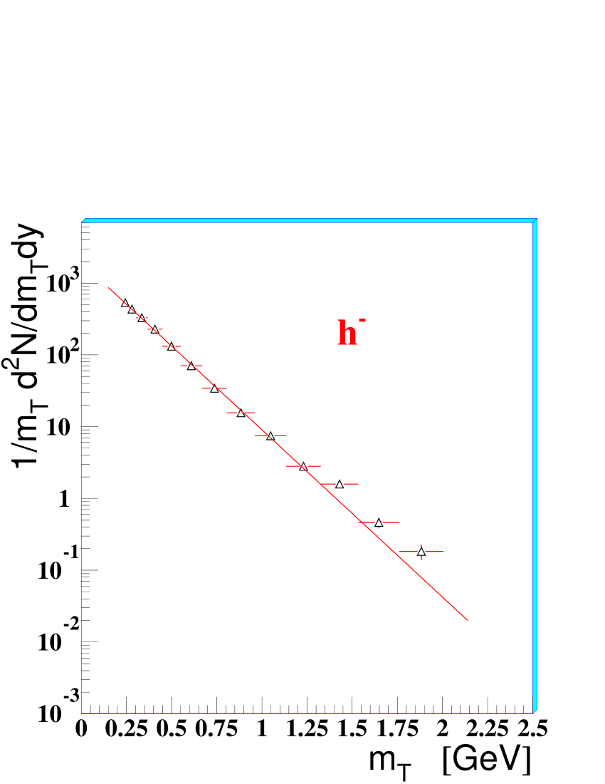
In the hydro-dynamical view, the apparent temperature is interpreted as due to the thermal motion coupled with a collective transverse flow of the fireball components [4], and it depends on $m_{\tt T}$. At a given ${m_{\tt T}}_{0}$ value, it can be calculated according to the formula [4]:

$$T_{\tt app}({m_{\tt T}}_{0})=\left[\lim_{m_{\tt T}\rightarrow{m_{\tt T}}_{0}}\frac{{\rm d}}{{\rm d}m_{\tt T}}(\log\frac{{\rm d}N}{{\rm d}m_{\tt T}^{2}})\right]^{-1}$$ (3)

This expression simplifies for $m_{\tt T}\gg m$: the apparent temperature is simply blue-shifted by the collective dynamics

$$T_{\tt app}=T\sqrt{\frac{1+\langle\beta_{\perp}\rangle}{1-\langle\beta_{\perp}\rangle}}$$ (4)

where $T$ is the freeze-out temperature and $\langle\beta_{\perp}\rangle$ is the average transverse flow velocity.

3.1 Centrality dependence

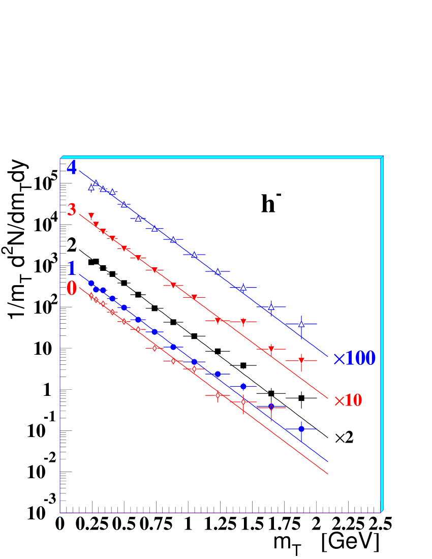
The transverse mass spectra of negative hadrons are shown in figure 3 for the five centrality classes defined in table 1: the inverse slope parameter $T_{\tt app}$ does not depend on centrality and its values are given in table 2.

Figure 3: Transverse mass spectra of negatively charged particles in Pb–Pb collisions at 40 $A$ GeV/$c$ for the five centrality classes of table 1. The spectra of class $2$, $3$ and $4$ have been scaled by factors $2$, $10$ and $100$, respectively, for display purposes.

Table 2: Inverse slopes (MeV) of the $m_{\tt T}$ distributions of $\tt h^{-}$ in Pb–Pb collisions at 40 $A$ GeV/$c$ for the five centrality classes defined in table 1. Systematic errors are estimated to be 8.5% for all centralities.

0	1	2	3	4
$186\pm 6$	$185\pm 3$	$185\pm 3$	$188\pm 3$	$187\pm 4$

4 Two-particle correlation

In this section we present the study of the Hanbury-Brown and Twiss correlation for negatively charged hadrons assumed to be pions (see section 4.1.2). An introduction to this topic and recent reviews of experimental results and theoretical developements can be found in references [10, 11].

The data will be analyzed in the framework of the hydro-dynamical inspired blast-wave model [4], which assumes cylindrical symmetry for an expanding fireball in local thermal equilibrium. Hydro-dynamics or parameterized models inspired by hydro-dynamics have shown to give a successful description of a number of observables, i.e. transverse momentum ($p_{\tt T}$) and rapidity ($y$) distributions, direct and elliptical flow, two-particle correlation functions (for recent reviews see, e.g., references [12]). The single set of free parameters of the model to be obtained from the HBT study is: the kinetic freeze-out temperature ($T$), the average transverse flow velocity ($\langle\beta_{\perp}\rangle$), the Gaussian radius of the cylindrical system ($R_{\rm G}$), the chaoticity of the pion emission ($\lambda$), the proper time of the freeze-out ($\tau_{f}=\sqrt{t^{2}_{f}-x^{2}_{f}}$) and the emission duration ($\Delta\tau$).

Experimentally, the correlation function can be defined as

$$C_{2}(q)=N\frac{S(q)}{B(q)}$$

where the signal $S(q)$ is the measured distribution of the relative four-momentum $q=p_{1}-p_{2}$ of two identical particles in one event and the background $B(q)$ is the reference distribution built by pairing two particles taken from different events. For each pair of negative hadrons in the signal, there are about 15 pairs in the background, formed from events of similar multiplicity, so that the error on $C_{2}$ is statistically dominated by the signal. The normalization factor $N$ is obtained by imposing that the integral of $C_{2}(q)$ be equal to unit in the region of large $q$, where there is neither quantum (i.e. Bose-Einstein) nor other (e.g. Coulomb) correlations.

The relative momentum $q$ is measured on a pair-by-pair basis relative to the out–side–long reference, which is a Cartesian system defined by choosing the long axis along the beam direction; the out and side axes lay in the transverse plane with the former aligned with the average transverse momentum of the pair and the latter perpendicular to the other two axes. With respect to the laboratory system, the out–side–long reference is boosted pair-by-pair along the long axis in such a way to bring to rest the pair in that direction: in the literature this boosted system is usually referred to as the Longitudinally Co-Moving System (LCMS). In this reference system, the correlation function is parameterized according to a three-dimensional Gaussian function modified by the addition of an out–long cross-term:

$$C_{2}=1+\lambda\exp\left[-R_{\tt out}^{2}q_{\tt o}^{2}-R_{\tt side}^{2}q_{\tt s}^{2}-R_{\tt long}^{2}q_{\tt l}^{2}-2|R_{\tt ol}|R_{\tt ol}q_{\tt o}q_{\tt l}\right]$$ (5)

Such a parameterization is suited for central collisions which are azimuthally symmetric. In case of a peripheral collision, the azimuthal symmetry is evidently broken; however it is recovered when building the correlation function from particles accumulated over many events with random impact parameters, which is our approach. The $\lambda$ parameter in equation 5 is referred to as the chaoticity parameter and it is expected to range in the interval $[0,1]$.

4.1 Study of the event sample properties

4.1.1 Acceptance region

The determination of the size and dynamical evolution of the system at freeze-out requires information about the dependence of the HBT radii on the mean momentum $\vec{K}=\frac{1}{2}(\vec{p}_{1}+\vec{p}_{2})$ of the pair. This can be parameterized by its transverse component and the pair rapidity (computed assuming the pion mass):

$$K_{\tt T}=\frac{1}{2}\sqrt{(p_{y1}+p_{y2})^{2}+(p_{z1}+p_{z2})^{2}}$$ (6)

$$Y_{\pi\pi}=\frac{1}{2}\log\frac{E_{1}+E_{2}+p_{x1}+p_{x2}}{E_{1}+E_{2}-p_{x1}-p_{x2}}$$ (7)

With this in mind, our (two-particle) acceptance window, which is shown in figure 4, has been binned in 20 rectangles in each of which the correlation function $C_{2}(q)$ has been measured independently.

Figure 4: Two-particle acceptance window used in the Hanbury-Brown and Twiss analysis. The correlation function has been measured in each of the 20 rectangles patching the window together. The $K_{\tt T}$ and $Y_{\pi\pi}$ average values, measured over the rectangles, are reported in table 3. The dotted line is drawn at $Y_{\pi\pi}=y_{\tt cm}$.

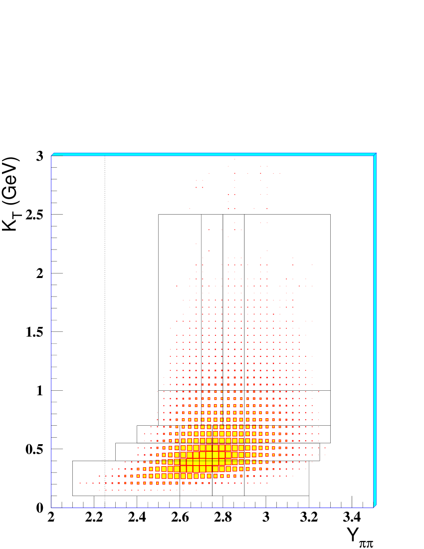
Table 3 displays the average values of the $K_{\tt T}$ and $Y_{\pi\pi}$ distributions in each of the 20 bins used for the analysis.

Table 3: Averages of the $K_{\tt T}$ (uppermost number in the cells, in ${\rm GeV}/c$ units) and $Y_{\pi\pi}$ (bottom numbers, in blue on-line) distributions in the 20 rectangles of figure 4

	$\begin{array}[]{cc}1.157\\ {\color[rgb]{0,0,1}2.65}\end{array}$	$\begin{array}[]{cc}1.162\\ {\color[rgb]{0,0,1}2.75}\end{array}$	$\begin{array}[]{cc}1.163\\ {\color[rgb]{0,0,1}2.85}\end{array}$	$\begin{array}[]{cc}1.175\\ {\color[rgb]{0,0,1}2.99}\end{array}$
	$\begin{array}[]{cc}0.804\\ {\color[rgb]{0,0,1}2.64}\end{array}$	$\begin{array}[]{cc}0.808\\ {\color[rgb]{0,0,1}2.75}\end{array}$	$\begin{array}[]{cc}0.809\\ {\color[rgb]{0,0,1}2.85}\end{array}$	$\begin{array}[]{cc}0.813\\ {\color[rgb]{0,0,1}2.98}\end{array}$
$\uparrow$	$\begin{array}[]{cc}0.610\\ {\color[rgb]{0,0,1}2.57}\end{array}$	$\begin{array}[]{cc}0.615\\ {\color[rgb]{0,0,1}2.68}\end{array}$	$\begin{array}[]{cc}0.617\\ {\color[rgb]{0,0,1}2.82}\end{array}$	$\begin{array}[]{cc}0.620\\ {\color[rgb]{0,0,1}2.97}\end{array}$
$K_{\tt T}$	$\begin{array}[]{cc}0.460\\ {\color[rgb]{0,0,1}2.55}\end{array}$	$\begin{array}[]{cc}0.468\\ {\color[rgb]{0,0,1}2.68}\end{array}$	$\begin{array}[]{cc}0.472\\ {\color[rgb]{0,0,1}2.82}\end{array}$	$\begin{array}[]{cc}0.478\\ {\color[rgb]{0,0,1}2.97}\end{array}$
	$\begin{array}[]{cc}0.305\\ {\color[rgb]{0,0,1}2.51}\end{array}$	$\begin{array}[]{cc}0.332\\ {\color[rgb]{0,0,1}2.67}\end{array}$	$\begin{array}[]{cc}0.345\\ {\color[rgb]{0,0,1}2.81}\end{array}$	$\begin{array}[]{cc}0.358\\ {\color[rgb]{0,0,1}2.95}\end{array}$
	$Y_{\pi\pi}\,\longrightarrow$

Additionally, in order to investigate the dynamics of the collision as a function of centrality, the whole analysis has been repeated in three centrality classes obtained from those defined in table 1: central ($3+4$), semi-central ($2$) and semi-peripheral ($0+1$), which correspond to the ranges of centrality 0–11%, 11–23% and 23–53%, respectively.

4.1.2 Contamination from non $\pi^{-}$–$\pi^{-}$ pairs

The correlation analysis presented here is based on pairs of negative hadrons ($\tt h^{-}$–$\tt h^{-}$), which are expected to be dominated by pairs of identical pions. The purity decreases with increasing $K_{\tt T}$: based on the results of NA49 [13] we estimate that at $K_{\tt T}\approx 0.3$ GeV/$c$ it is about 90%, at $K_{\tt T}\approx 0.8$ (1.2) GeV/$c$ it goes down to about 80% (65%). The main contamination comes from $\mathrm{\pi^{-}}$–$\mathrm{K^{-}}$pairs (from about 5% at $K_{\tt T}\approx 0.3$ GeV/$c$ to about 25% at $K_{\tt T}\approx 1.2$ GeV/$c$) and also from $\mathrm{K^{-}}$–$\mathrm{K^{-}}$pairs (up to $\approx$ 10% at $K_{\tt T}\approx 1.2$ GeV/$c$). Other combinations, e.g. $\mathrm{\pi^{-}}$–$\mathrm{\overline{p}}$ or $\mathrm{K^{-}}$–$\mathrm{\overline{p}}$, are negligible, the largest being about a few per cent for $\mathrm{\pi^{-}}$–$\mathrm{\overline{p}}$ at $K_{\tt T}\approx 1.2$ GeV/$c$.

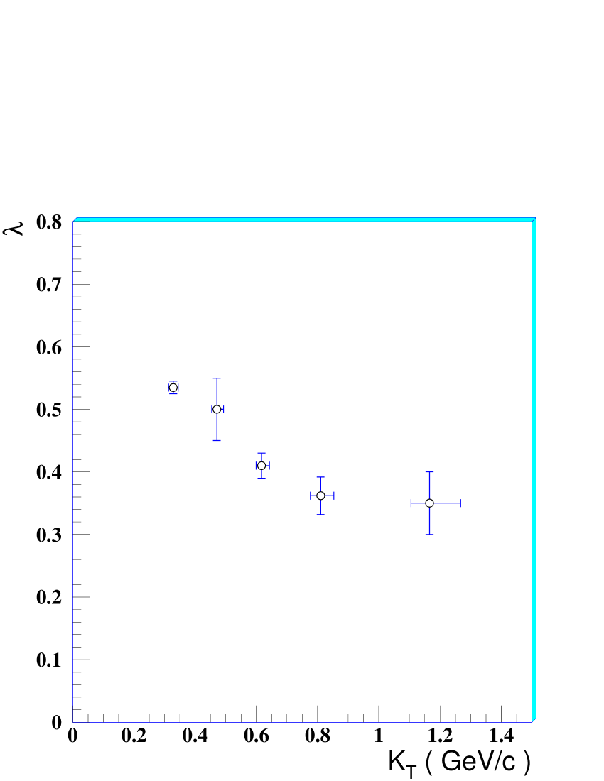
Excepting $\mathrm{K^{-}}$–$\mathrm{K^{-}}$pairs at high $K_{\tt T}$, misidentified particles thus lead to counting of unlike pairs which do not give rise to Bose-Einstein correlations. Moreover, in Pb–Pb collisions at $E_{\rm beam}=158$ GeV per nucleon the measured HBT radius parameters of the $\mathrm{K^{-}}$–$\mathrm{K^{-}}$ (and $\mathrm{K^{+}}$–$\mathrm{K^{+}}$) correlation functions [14] (NA49 Collaboration) are fully consistent with the published pion results and the hydro-dynamic expansion model. It has been shown in [15] (NA35 experiment), in [16] (NA49 experiment) and in [17] (WA97 experiment) that the main effect of particle misidentification is to reduce the value of the chaoticity parameter $\lambda$. Apart from particle misidentification which produces the strongest bias, the $\lambda$ parameter, shown in figure 5 as a function of $K_{\tt T}$, is also affected in a non-trivial way by resonance decays and other effects [18], which are expected to depend on the pair momentum. The $\lambda$ parameter, however, is not used for the reconstruction of the size and dynamical state of the source; the relevant source parameters are affected to the level of a few per cent only.

Figure 5: The chaoticity parameter $\lambda$ as a function of $K_{\tt T}$ for the most central 53% of the Pb–Pb cross-section. Statistical errors are shown.

4.1.3 Two-track resolution

The detector’s ability to distinguish a pair of close tracks from a single track decreases with decreasing track separation, depending on the Si-pixel size. The correction for this inefficiency, applied pair-by-pair to the signal distribution $S(q)$, was calculated via a Monte Carlo simulation by reconstructing a sample of (generated) two-tracks events embedded in real ones. The maximum inefficiency was found to be $\approx$10% (relative to high $q$ pairs) for pairs populating the 10-MeV-wide bin of the correlation functions centred at $q=0$ and it goes to zero outside that bin.

4.1.4 Track splitting

The possibility of ghost tracks in the data sample has been investigated. Fake tracks might be produced by the reconstruction algorithm due to, e.g., allowing track candidates to share several clusters. To avoid such a bias, tracks have been selected by requiring them to have clusters in more than 80% of the telescope planes and less than 30% of the clusters shared with other tracks. As a final check, Monte Carlo events have been simulated by generating a sample of $\mathrm{\pi^{-}}$ distributed in phase-space according to the measured double differential cross-section of equation 2. Then, the simulated events have been reconstructed using the same algorithm as for real events. Three tracks only have been reconstructed with one associated ghost out of 250K generated tracks which pass through the pixel telescope. This effect is therefore negligible.

4.1.5 Momentum resolution

The quality of a correlation measurement is determined by the resolution of the two-particle momentum difference (“relative momentum”) $q$. The relative momentum resolution was studied using a Monte Carlo chain based on the simulation code GEANT [19]. As listed in table 4, we have estimated that the relative momentum projections $q_{\tt s}$ and $q_{\tt l}$ (the latter evaluated in the LCMS system) are measured in this analysis with an error not larger than about $20\,{\rm MeV}/c$ over our two-particle acceptance window. The $q_{\tt o}$ projection, on the other hand, shows a stronger $K_{\tt T}$ dependence, which can introduce an important contribution to the systematics errors on the extracted HBT radii, as discussed below.

Table 4: The resolution of relative momentum components $q_{\tt o}$, $q_{\tt s}$ and $q_{\tt l}$ (MeV/$c$) in the LCMS system as a function of $K_{\tt T}$ (GeV/$c$).

	$K_{\tt T}<0.5$	$0.5<K_{\tt T}<1.0$	$K_{\tt T}>1.0$
$q_{\tt o}$	22	52	110
$q_{\tt s}$	15	18	21
$q_{\tt l}$	10	11	13

4.1.6 Coulomb correction

The observed two-particle correlation is expected to result from two different contributions, the Bose-Einstein effect and the Coulomb interaction. The Coulomb interaction between particles of same charge sign is repulsive, thus depleting the two-particle correlation function at small relative momenta. Two methods have been considered to correct for the Coulomb interaction.

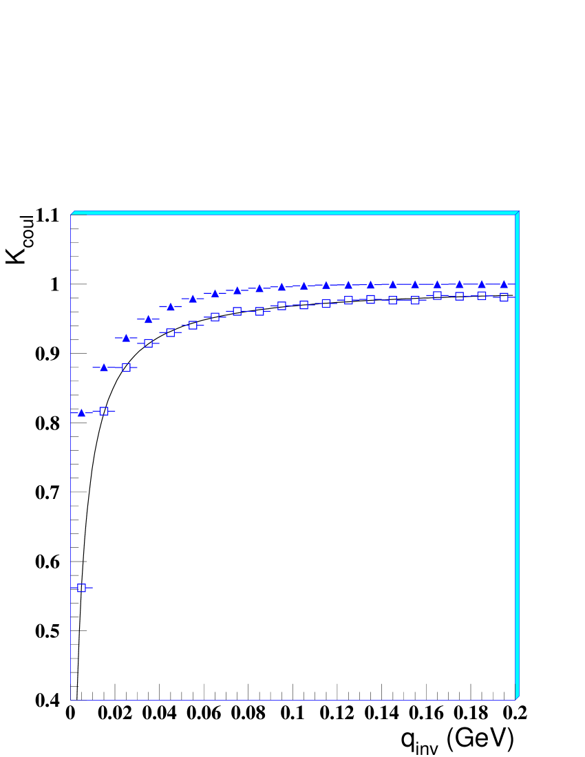
A standard procedure consists in applying $q_{\rm inv}$-dependent weights to each pair in the background distribution $B(q)$ to get the Coulomb corrected correlation function:

$$C_{2}^{corr}(q)=N\frac{S(q)}{K_{\rm Coul}(q_{\rm inv})\cdot B(q)}=$$ (8)

$$1+\lambda\exp\left[-R_{\tt out}^{2}q_{\tt o}^{2}-R_{\tt side}^{2}q_{\tt s}^{2}-R_{\tt long}^{2}q_{\tt l}^{2}-2|R_{\tt ol}|R_{\tt ol}q_{\tt o}q_{\tt l}\right]$$

where $K_{\rm Coul}$ is the squared Coulomb wave-function integrated over the whole source and $q_{\rm inv}=\sqrt{\vec{q}^{2}-q_{0}^{2}}$.

Bowler and Sinyukov pointed out [20] that the correction procedure should be different in the case where not all particle pairs in the signal distribution are subject to the Coulomb correlation. The argument here is that if physics (or detector) related effects lead to a reduction of the observed quantum correlation strength, then the same effects also lead to a similar reduction of the Coulomb repulsion. Therefore, the strength of the Coulomb correction applied to the data should be linked to the experimentally observed $\lambda$ parameter. This method has been implemented recently by the CERES [21], PHOBOS [22] and STAR [23] Collaborations. The correlation function in this procedure is fitted to

$$C_{2}(q)=\frac{S(q)}{B(q)}=(1-\lambda)+$$ (9)

$$\lambda\cdot K_{\rm Coul}(q_{\rm inv})\cdot\left[1+\exp(-R_{\tt out}^{2}q_{\tt o}^{2}-R_{\tt side}^{2}q_{\tt s}^{2}-R_{\tt long}^{2}q_{\tt l}^{2}-2|R_{\tt ol}|R_{\tt ol}q_{\tt o}q_{\tt l})\right]$$

where $K_{\rm Coul}(q_{\rm inv})$ is the same as in the standard procedure. We argue that this alternative method is appropriate when the correlation function is measured with a negligible contamination of non-identical particle pairs; in fact the particles of these pairs would Coulomb interact in the signal and would not in the background distribution. Therefore we consider it only as an alternative method to control possible systematic errors on the HBT radii due to the Coulomb correction, as discussed later.

For both procedures, three kinds of pion emitting sources have been considered with a method similar to that described in reference [17]:

• a point-like source (in space–time);

• a static Gaussian source;

• an expanding source, parameterized according to the same blast-wave model [4] used to describe the data.

The point-like source was used for comparison with the analytical Gamow factor [24, 25] for the sake of validation of the method. A static Gaussian source with a radius of 5 fm yields a Coulomb correction smaller than the Gamow factor and slightly larger than that obtained for the expanding source. The computation of the Coulomb correction for the expanding source requires knowledge of the source parameters, which are not known a priori but should be obtained from the correlation study. Therefore an iterative procedure has been used, as discussed in reference [17], starting with the following values for the blast-wave model freeze-out parameters (to be discussed later): $T=120$ MeV, $\langle\beta_{\perp}\rangle=0.4$, $R_{G}=5$ fm, $\tau_{\rm f}=5$ fm/$c$ and $\Delta\tau=1$ fm/$c$. The results for the model parameters become stable after the first iteration.

In figure 6 the correction factor $K_{\rm Coul}$ for an expanding source, which has been used in this analysis, is shown superimposed to the correction for a point-like source and to the Gamow factor.

Figure 6: Coulomb correction for an expanding source (full triangles, see text for details) and for a point-like source (open squares) as compared to the Gamow factor (full line).

4.2 Multidimensional fit

Equation 5 has been fitted to the corrected correlation functions by maximizing the negative logarithmic likelihood function:

$$-2\log\ L(\vec{R})=2\sum_{i}[C_{i}B_{i}-S_{i}\log(C_{i}B_{i})+\log(S_{i}!)]$$ (10)

where $C_{i}$ is the theoretical value of the correlation function for a given set of parameters $\vec{R}=(\lambda,R_{\tt out},R_{\tt long},R_{\tt side},R_{\tt ol})$ in the $i^{\rm th}$ bin of $q$ and $S_{i}$ and $B_{i}$ are, respectively, the distribution of signal and background in that bin.

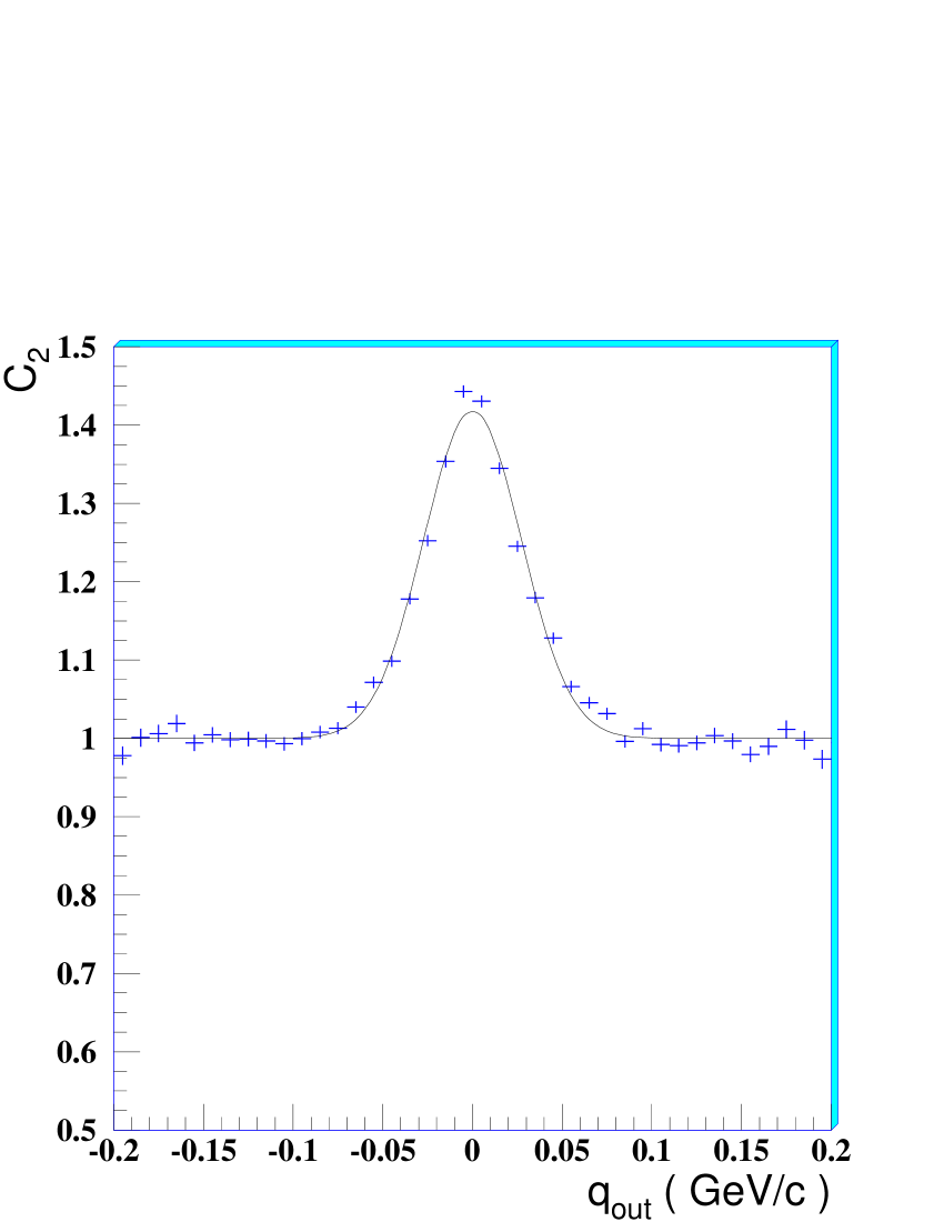
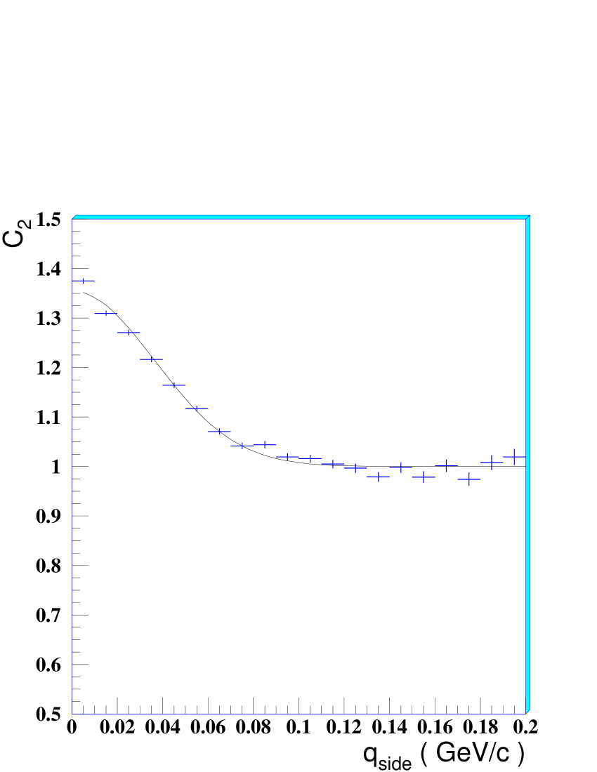
Two checks on the fit quality have been performed. First, the $\chi^{2}/{\rm ndf}$–values are calculated on the three-dimensional correlation function using the parameters corresponding to the maximum likelihood fit and are found to be distributed around unity. Second, the projections of the 3-dimensional correlation function onto each momentum difference component, with narrow cuts on the other components, have been fitted by the least-squares method to a Gaussian function, yielding results consistent with the results of the 3-dimensional fits. A typical sample of these projections is shown in figure 7 where the correlation function has been integrated along the other $q_{j}$ components in the intervals $|q_{j}|<30\,{\rm MeV}$.

Figure 7: Projections of the $\tt h^{-}$–$\tt h^{-}$ correlation function measured using Cartesian parameterization for pair rapidities $2.30<Y_{\pi\pi}<3.25$ and pair transverse momenta $0.40<K_{\tt T}<0.55$ GeV/c. Full curves are the result of a least-squares fit to a Gaussian function (see the text).

4.3 Systematic errors

The main sources of systematic uncertainties on the HBT radii are attributed to three previously mentioned effects, namely, with decreasing importance, (i) the momentum resolution, (ii) the Coulomb correction procedure and (iii) the double-track resolution.

The systematic error due to the finite momentum resolution, which depends on the transverse momentum of the pair, has been evaluated by a Monte Carlo simulation with the following approach. A sample of pion pairs was generated, whose particles are extracted from the phase-space $\frac{{\rm d}N}{{\rm d}p^{\mu}\,{\rm d}x^{\nu}}$ of the expanding model with the parameters specified in section 4.1.6. The momentum-dependent part of this particle phase-space distribution is then propagated through the apparatus to take into account the experimental acceptance and reconstruction inefficency, in order to end up with the raw measured momentum distribution $\frac{{\rm d}N}{dp^{\mu}}^{\rm raw}$. Quantum and other correlations are introduced in a second stage using the method outlined in reference [26]. The same procedure is repeated for a second sample of pairs, obtained from the first one by smearing the momentum distribution according to the experimental momentum resolution. The variations of the extracted HBT radii provide an estimate of the systematic errors.

As discussed in section 4.1.6, two Coulomb correction procedures have been implemented, each with different assumptions about the source properties (its space-time extent, static or expanding source, etc.). The differences in the HBT radii obtained with the different methods allow us to estimate a contribution to the systematic error of 10% for $R_{\tt out}$, $R_{\tt side}$ and $R_{\tt long}$, and of 5% for the cross-term $R_{\tt ol}$.

The last source of systematical errors can be associated to the double-track resolution and arises from the finite statistics of Monte Carlo events generated to correct for this effect. It is of the order of a few per cent for all the radii.

In table 5 the total systematic errors are given in percentages as a function of $K_{\tt T}$.

Table 5: Percentages of systematic errors on the HBT radii for three intervals of $K_{\tt T}$.

	$K_{\tt T}<0.5$	$0.5<K_{\tt T}<1.0$	$K_{\tt T}>1.0$
$R_{\tt out}$	12	14	16
$R_{\tt side}$	10	10.5	11
$R_{\tt long}$	11	11.5	13
$R_{\tt ol}$	11.5	15	28

5 Results and discussion

5.1 Longitudinal expansion

The cross-term $R_{\tt ol}$ provides information about the longitudinal expansion of the system; e.g. for a longitudinal Bjorken-like expansion [27] $R_{\tt ol}$ should vanish in the LCMS system at mid-rapidity [28]. Figure 8 shows the $K_{\tt T}$ dependence of the $R_{\tt ol}$ parameters for the most central 53% of the Pb–Pb inelastic cross-section (“all”) and for the three centrality classes specified at the end of section 4.1.1. The statistical and systematic errors are indicated in these and following plots with bars and shadow boxes (green on-line), respectively.

Figure 8: The $R_{\tt ol}$ cross-term as a function of $K_{\tt T}$ for the most central 53% of the Pb–Pb cross-section (top-left panel) and for individual centrality classes 0–1 (top-right), 2 (bottom-left) and 3-4 (bottom right) of table 1. The bars and the boxes show the statistical and systematic errors, respectively.

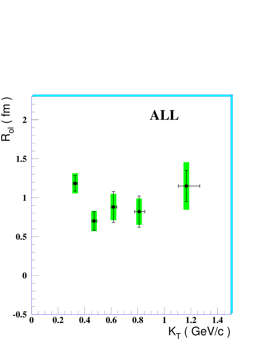
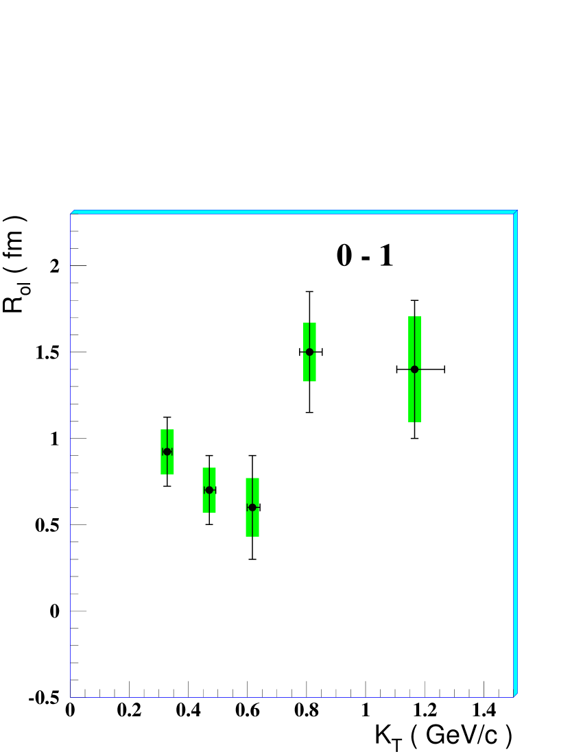
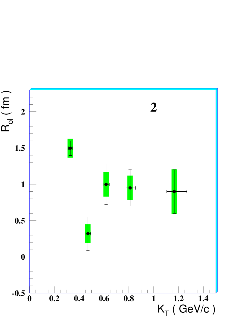
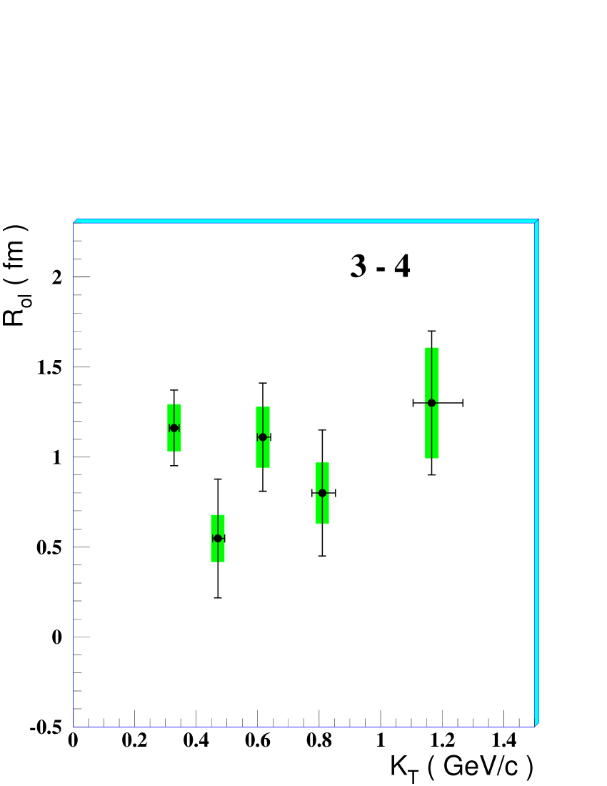
Unfortunately, in most of the recent experimental works about HBT correlations in heavy ion collisions scarce consideration is given to the study of this parameter. Indeed, the cross term is often not used in the Cartesian parameterization (equation 5) or, when used, it is frequently assumed to be of a given sign (e.g. positive in the LCMS system). Such an approach could be justified at RHIC energies near mid-rapidity, where the Bjorken model should provide a good description of the longitudinal expansion; it is not at lower energy. Instead, the longitudinal dynamics is derived from the Yano-Koonin-Podgoretskii parameterization [29] of the HBT correlation function

$$C_{2}(q)=1+\lambda\exp\left[-R^{2}_{\perp}q^{2}_{\perp}-\gamma^{2}_{\rm yk}(q_{\parallel}-v_{\rm yk}q_{\rm 0})^{2}R^{2}_{\parallel}-\gamma^{2}_{\rm yk}(q_{\rm 0}-v_{\rm yk}q_{\parallel})^{2}R^{2}_{\rm 0}\right]$$ (11)

where $R_{\perp}$, $R_{\parallel}$, $R_{\rm 0}$ are called the “YKP radii”, although $R_{\rm 0}$  has temporal dimension (${\rm fm}/c$); $v_{\rm yk}$, called “Yano-Koonin velocity”, is measured in units of c and $\gamma_{\rm yk}=(1-v_{\rm yk}^{2})^{-1/2}$. In fact, in this parameterization the $v_{\rm yk}$ parameter can be easily related, under some approximations, to the longitudinal flow velocity of the expanding source [30, 31].

The set of parameters of the Yano-Koonin parameterization can be computed from that of the Cartesian parameterization (and vice versa) via analytical relations [30, 31, 32]. In particular, for the Yano-Koonin velocity the relation is:

$$v_{\rm yk}=\frac{A+B}{2C}\left[1-\sqrt{1-\left(\frac{2C}{A+B}\right)^{2}}\right]$$ (12)

where in the LCMS system, due to the vanishing of the longitudinal pair velocity, $A=\frac{R_{\tt out}^{2}-R_{\tt side}^{2}}{\beta^{2}_{\perp}}$, $B=R_{\tt long}^{2}$ and $C=-|R_{\tt ol}|R_{\tt ol}$; finally $\beta_{\rm T}$ is the transverse component of the pair velocity $\vec{\beta}\simeq\vec{K}/K^{0}$.

From the Yano-Koonin velocity, one can compute its associated rapidity $Y_{\rm yk}=\frac{1}{2}\ln(\frac{1+v_{\rm yk}}{1-v_{\rm yk}})$, which is often plotted as a function of the pair rapidity to study the longitudinal expansion (see, e.g., references [16, 22]). In figure 9 we plot this quantity, evaluated in the laboratory system, as a function of the pair rapidity $Y_{\pi\pi}$ also given in the same frame: $Y_{\rm yk}^{\rm lab}=Y_{\rm yk}^{\rm LCMS}+Y_{\pi\pi}$. Statistical and systematic errors, shown at the 1$\sigma$ confidence level, have been propagated from those of the out-side-long HBT radii. In these plots the correlation functions have been integrated in the range $0.1<K_{\tt T}<0.7$ GeV/$c$ where the $\langle K_{\tt T}\rangle$ has been evaluated to be 0.36, 0.41, 0.51 and 0.58 GeV/$c$, for the data points at $Y_{\pi\pi}=$ 2.53, 2.68, 2.82 and 2.97, respectively.

Figure 9: The Yano-Koonin rapidity $Y{\tt yk}$ as a function of the pair rapidity $Y_{\pi\pi}$ measured in the interval $0.1<K_{\tt T}<0.7$ GeV/$c$ (see text for the averages of $K_{\tt T}$ in each bin). The most central 53% of the Pb–Pb cross-section (top-left panel) and the individual centrality classes 0–1 (top-right), 2 (bottom-left) and 3-4 (bottom right) of table 1 are shown. Full circles are data, open circles are data reflected about mid-rapidity. Statistical and systematic errors are indicated with line bars and shaded boxes (green on-line), respectively.

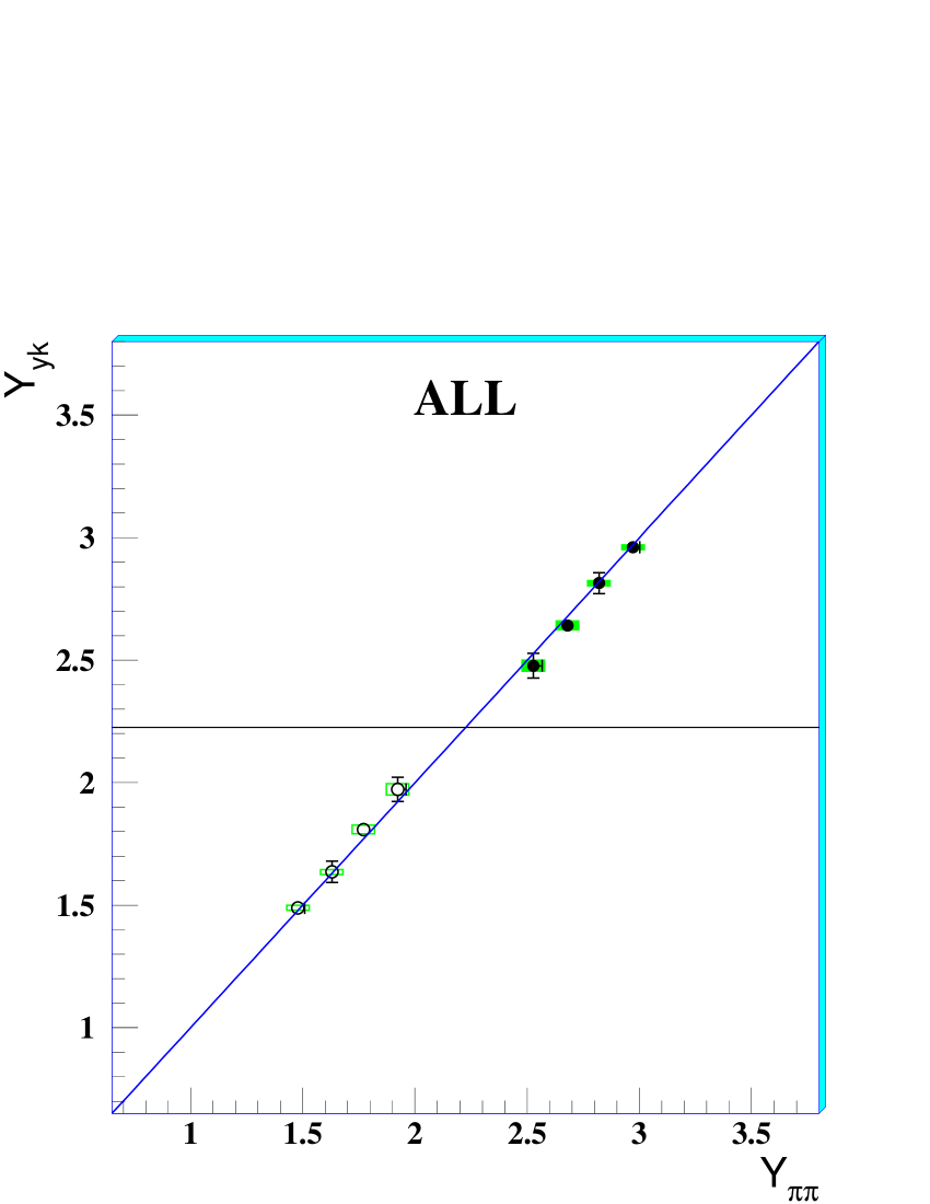
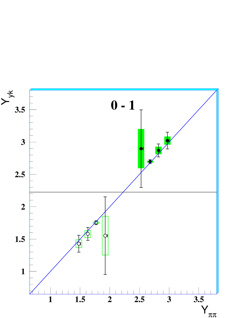
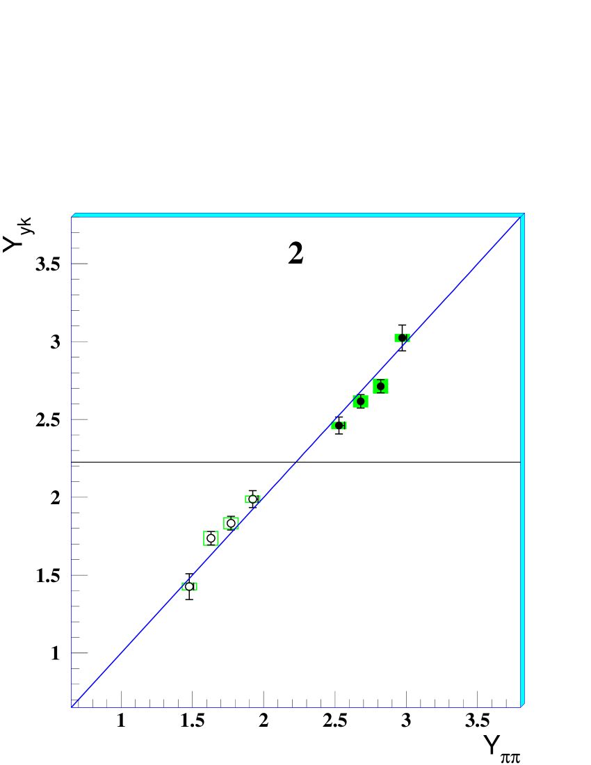
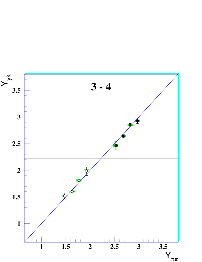
The source rapidity scales with the rapidity of the pair, indicating the presence of strong position-momentum correlations. A static source would exhibit no correlation and would correspond to a horizontal line at the rapidity of the center of mass. ($Y_{\tt yk}=y_{\tt cm}$). A source with strong dynamical correlations would correspond to a straight line along $Y_{\tt yk}=Y_{\pi\pi}$. The data are consistent with the latter scenario: particles emitted at a given rapidity are produced by a source moving collectively at the same rapidity.

5.2 Transverse expansion

The $\vec{K}$-dependence of $R_{\tt side}$ provides information about the transverse expansion of the source and its geometrical transverse size at freeze-out [33].

In figure 10 we plot $R_{\tt side}$ as a function of $K_{\tt T}$ for the integrated centrality range and for the three centrality classes used in this HBT analysis.

Figure 10: The $R_{side}$ radius as a function of $K_{\tt T}$ for the most central 53% of the Pb–Pb cross-section (top-left panel) and for individual centrality classes 0–1 (top-right), 2 (bottom-left) and 3-4 (bottom right) of table 1. Statistical and systematic errors are indicated with line bars and shaded boxes (green on-line), respectively.

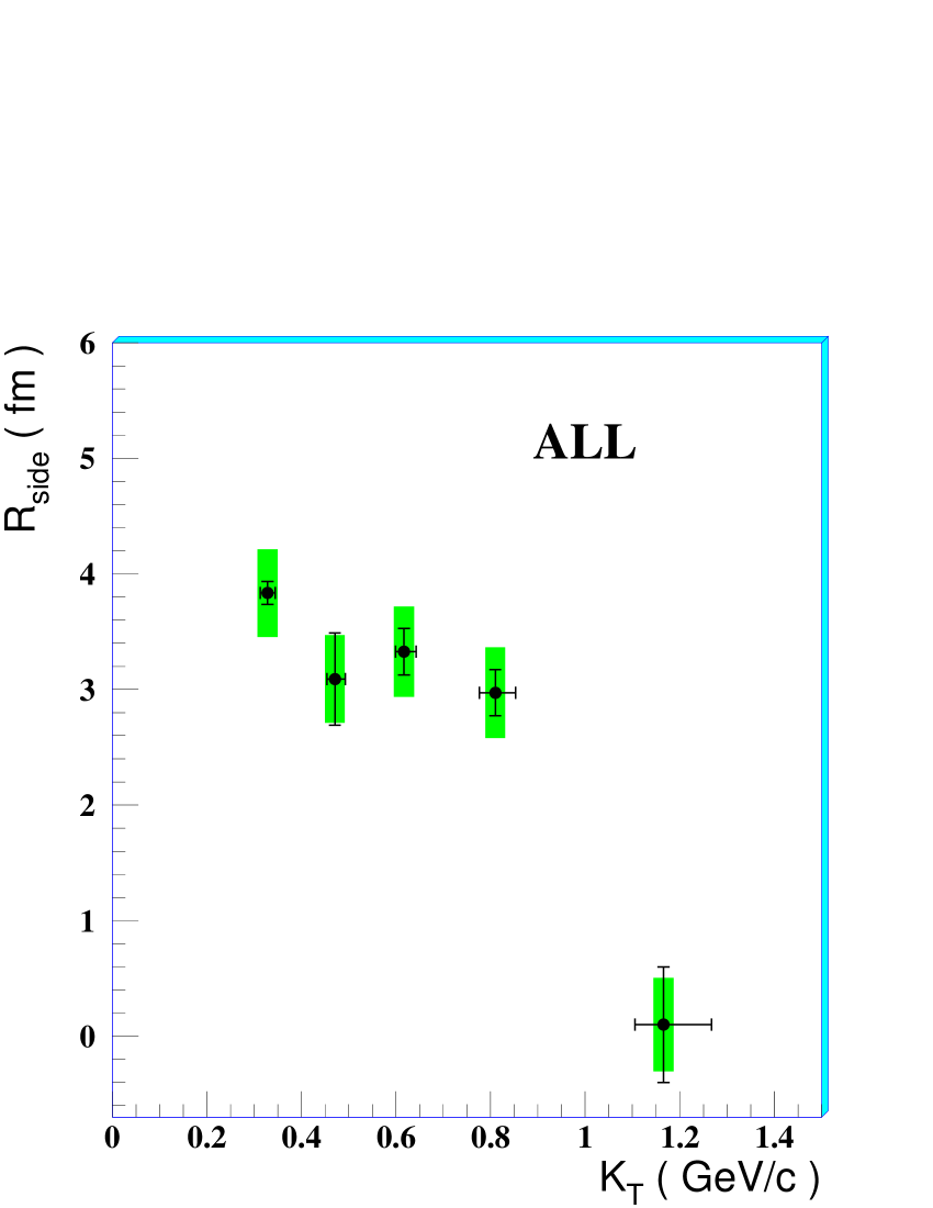
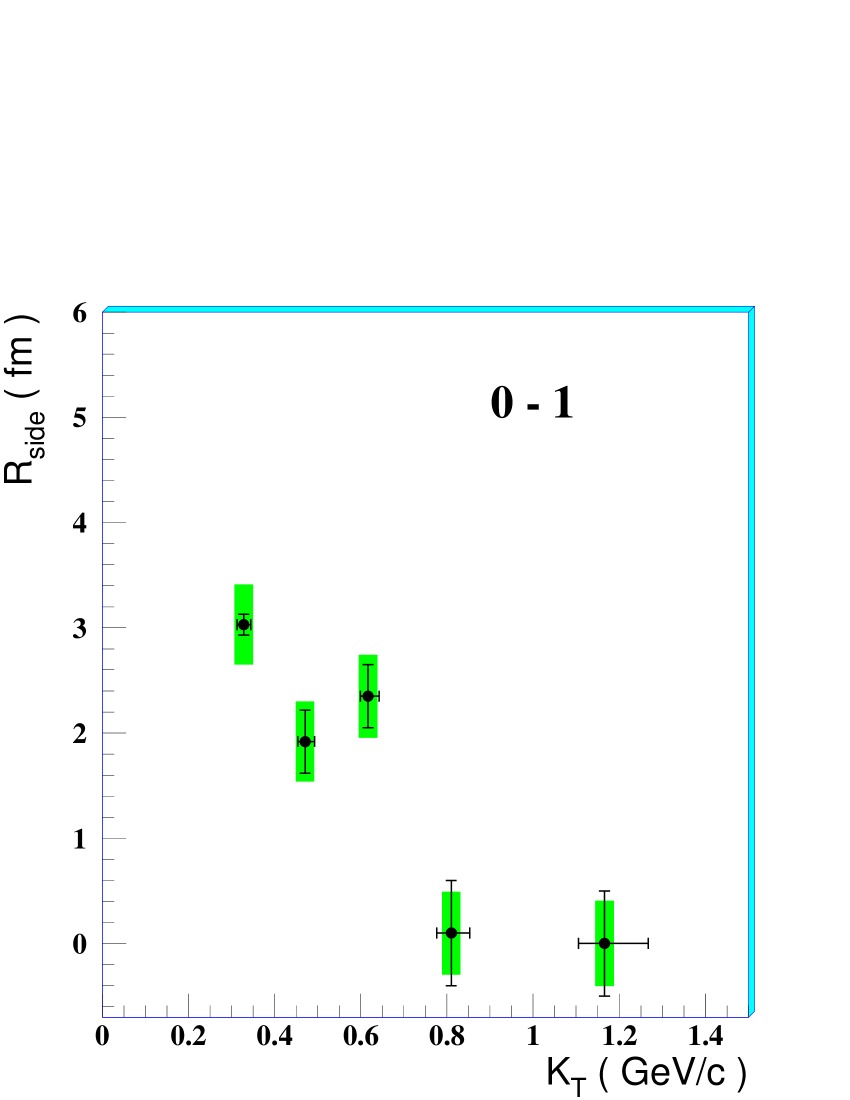
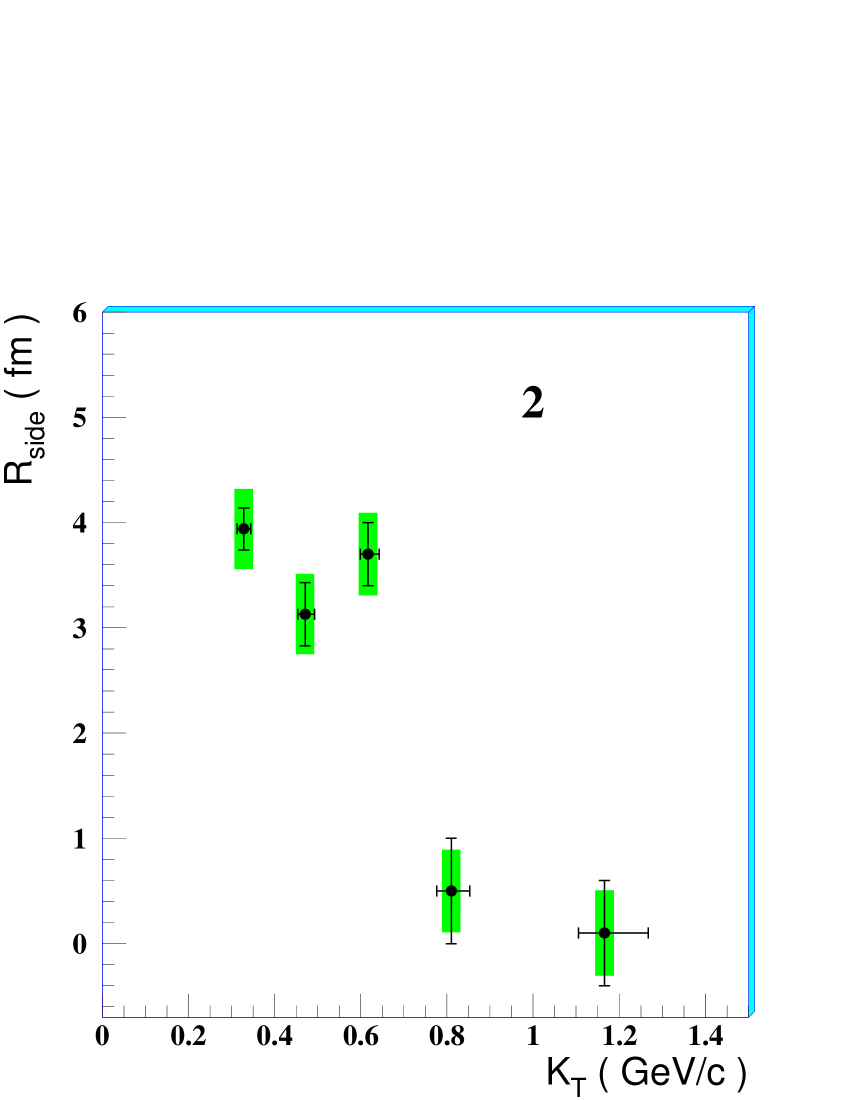
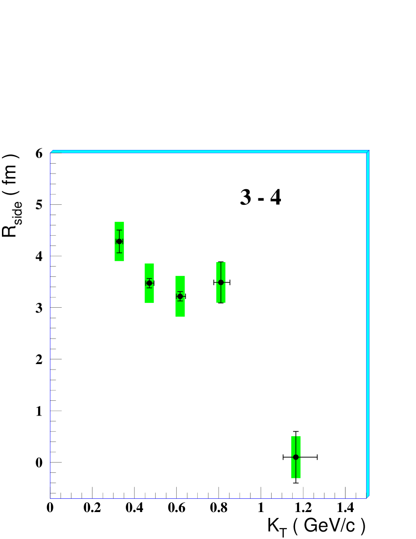
In the hydro-dynamical view, the decrease of $R_{\tt side}$ with increasing $K_{\tt T}$ is due to the collective expansion in the transverse direction; the dependence of $R_{\tt side}$ on the pair momentum $\vec{K}$ can be parameterized by the formula [33, 34]

$$R_{\tt side}(K_{\tt T},Y_{\pi\pi})=\frac{R_{G}}{\sqrt{1+M_{\rm T}\frac{\beta_{\perp}^{2}}{T}\cosh(Y_{\rm yk}-Y_{\pi\pi})}}$$

where $M_{\rm T}=\sqrt{K_{\tt T}^{2}+m_{\pi}^{2}}$, $R_{\rm G}$ is equal to the transverse geometric (Gaussian) radius of the source times $1/\sqrt{2}$, $T$ is the freeze-out temperature and $\beta_{\perp}$ the slope of the (linear) transverse flow velocity profile: $\beta_{\perp}(r)=\beta_{\perp}\frac{r}{R_{\rm G}}$. A fit of equation 5.2 to the experimental data points provides the model parameter $R_{\rm G}$ and the ratio $\frac{\beta_{\perp}^{2}}{T}$; they are given in table 6.

Table 6: The transverse geometric parameter $R_{G}$ and the ratio $\beta^{2}_{\perp}/T$, $T$ being the freeze-out temperature.

Centrality	$R_{G}\;({\rm fm})$	$\frac{\beta_{\perp}^{2}}{T}\;({\rm GeV}^{-1})$
ALL	$5.7\pm 0.9$	$2.9\pm 1.4$
0-1	$4.3\pm 0.9$	$2.7\pm 1.7$
2	$6.9\pm 2.2$	$5.4\pm 3.3$
3-4	$6.6\pm 1.5$	$4.1\pm 2.6$

The measurement of the ratio $\frac{\beta_{\perp}^{2}}{T}$ determines an allowed region for the pair of variables $\langle\beta_{\perp}\rangle$ and $T$, the former being computed from the linear slope $\beta_{\perp}$ by assuming a uniform particle density of the source. Those allowed regions, at the 1$\sigma$ confidence level, are shown in figure 11; they correspond to the wide bands with positive slopes (in black on-line).

Figure 11: Contour plots at 1$\sigma$ confidence level (statistical error) in the $\langle\beta_{\perp}\rangle$–$T$ freeze-out parameter space, see text for details.

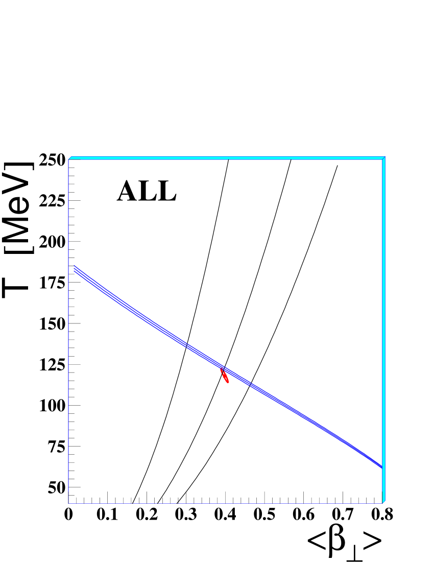
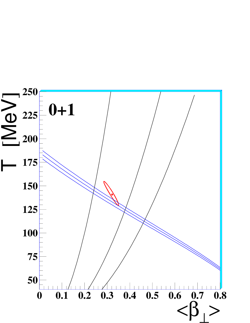
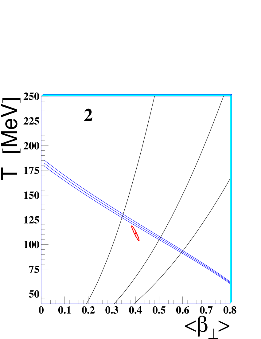
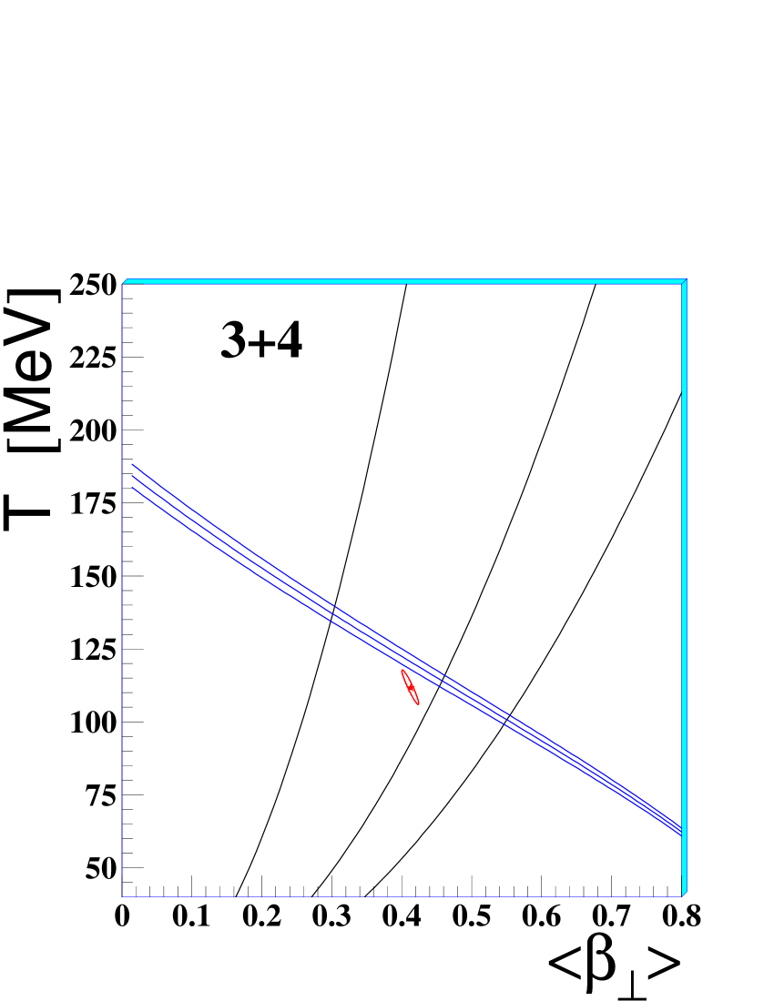
In order to disentangle the two parameters, we followed a technique first used by the NA49 Collaboration [16], where the measured single-particle $m_{\tt T}$ spectra are exploited. In this approach, the inverse slope parameters of the $m_{\tt T}$ distributions are interpreted according to the blue-shift formula 4, as discussed in section 3. This independent measurement provides another allowed region in the freeze-out parameter space, which corresponds to the narrow bands with negative slopes of figure 11 (blue on-line). The disentangled values for $T$ and $\langle\beta_{\perp}\rangle$ are reported in table 7.

Table 7: The freeze-out temperature $T$ and the average transverse flow velocity $\langle\beta_{\perp}\rangle$ as obtained from the study of negatively charged hadrons.

Centrality	$T({\rm MeV})$	$\langle\beta_{\perp}\rangle$
ALL	$122^{+15}_{-10}$	$0.40^{+0.07}_{-0.10}$
0-1	$125^{+20}_{-13}$	$0.37^{+0.10}_{-0.15}$
2	$106^{+22}_{-13}$	$0.50^{+0.10}_{-0.16}$
3-4	$114^{+22}_{-14}$	$0.45^{+0.10}_{-0.15}$

In figure 11 we also show the 1$\sigma$ confidence regions obtained from the blast-wave analysis of the $m_{\tt T}$ spectra of singly-strange particles ($\mathrm{K^{0}_{S}}$, $\mathrm{\Lambda}$ and $\mathrm{\overline{\Lambda}}$) [3]. They correspond to the small closed contours (red on-line) of figure 11, with the markers indicating the optimal fit locations. Our results thus suggest compatible freeze-out conditions for singly-strange particles and $\tt h^{-}$ (mainly negative pions) in Pb–Pb collisions at 40 $A$ GeV/$c$. On the other hand, the analysis of the transverse mass spectra of multiply-strange hyperons ($\mathrm{\Xi^{-}}$ and $\mathrm{\Omega^{-}}$) suggested that for the same colliding system these particles may undergo an earlier freeze-out than singly-strange particles [3].

Postponing to the next section a global discussion about these results, we note here that the most peripheral class 0–1 features a smaller transverse freeze-out radius, a lower transverse expansion velocity and a higher temperature. This suggests an expansion on a smaller scale; the higher temperature at the freeze-out may be interpreted as the remnant of an earlier decoupling of the expanding system. Such a centrality dependence of the freeze-out parameters is well established at the SPS and RHIC both from studies of the transverse mass spectra [3, 7, 35, 36, 37] and from HBT analyses [17, 21, 23, 38].

5.3 Temporal characterization of the expansion

Two parameters characterize the temporal evolution of the expansion dynamics, the proper time $\tau$ of the kinetic freeze-out and the duration of the pion emission $\Delta\tau$.

5.3.1 Proper time of freeze-out

Information about the evolution time-scale of the source, or proper time of freeze-out, can be extracted from the $\vec{K}$-dependence of the $R_{\tt long}$ radius. In figure 12 we show the $K_{\tt T}$ dependence of $R_{\tt long}$. We have fitted this parameter to a formula first suggested by Sinyukov and collaborators [39] and then improved by Chapman et al [33]:

$$R_{\tt long}(K_{\tt T},Y_{\pi\pi})=\sqrt{\frac{T}{m_{\tt T}}}\frac{\tau_{\rm f}}{\cosh(Y_{\rm yk}-Y_{\pi\pi})}$$

This formula assumes an instantaneous freeze-out in proper time (i.e., $\Delta\tau$ = 0); such an approximation is justified by the small $\Delta\tau$ found in the present (see later) and similar analyses.

Figure 12: The $R_{long}$ radius as a function of $K_{\tt T}$. Statistical and systematic errors are indicated with line bars and shaded boxes (green on-line), respectively.

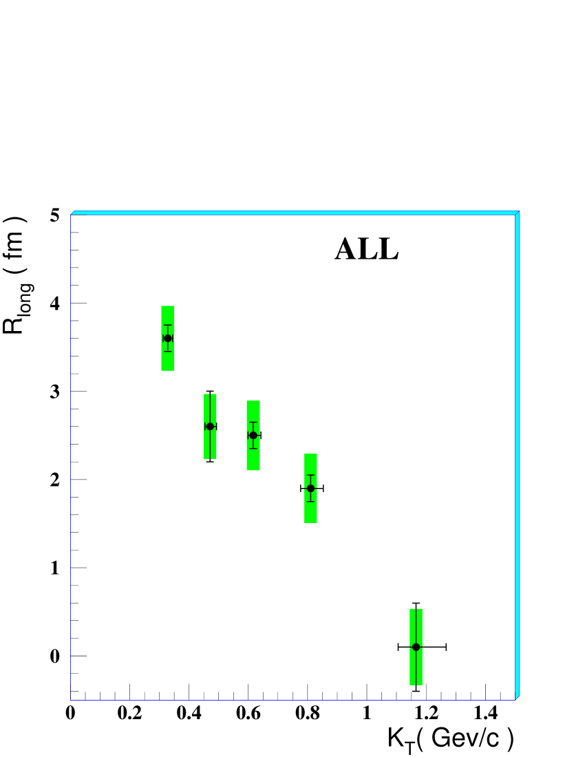
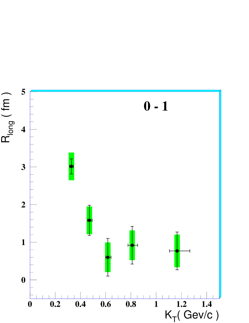
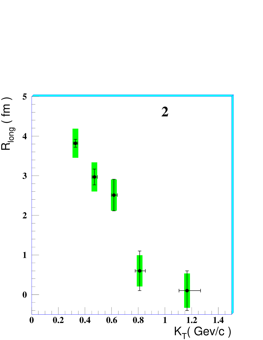
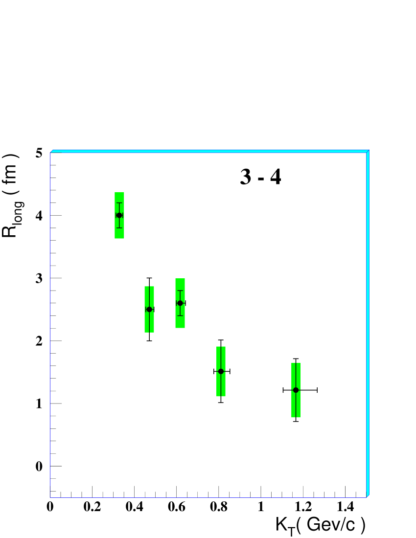
The results of the bidimensional fits of equation 5.3.1 to the experimental data are presented in table 8. In the fitting procedure we have used the freeze-out temperature determined from the analysis of the transverse dynamics, as discussed in section 5.2. This introduces an error which is kept separate in table 8 from that due to the $R_{\tt long}$ uncertainties.

Table 8: The proper time of freeze-out ($\tau$) in integrated centrality class (all) and for individual centrality classes. The second error is associated to the uncertainties on the value of $T$, as discussed in the text.

Centrality	$\tau$ (fm/$c$)
ALL	$6.7\pm 0.2\;^{+0.3}_{-0.3}$
0-1	$5.0\pm 0.3\;^{+0.3}_{-0.4}$
2	$7.2\pm 0.2\;^{+0.5}_{-0.7}$
3-4	$7.5\pm 0.3\;^{+0.6}_{-0.6}$

As observed for the transverse expansion, the class 0-1 shows an expansion on a smaller scale, its freeze-out (proper) time $\tau$ being significantly shorter than for the two most central classes.

5.3.2 Mean duration of the pion emission

It has been proposed that the existence of a strong first order phase transition and an accordingly long-lived mixed phase would be observable by a large outward radius $R_{\tt out}$ compared to $R_{\tt side}$, indicating a long duration of the pion emission $\Delta\tau$ [40, 41, 42, 43, 44, 45]:

$${\Delta\tau}^{2}=\frac{R_{\tt out}^{2}-R_{\tt side}^{2}}{\beta_{\rm T}^{2}}$$ (13)

where $\beta_{\rm T}$ is the average transverse velocity of the pair. The dependence of the $R_{\tt out}$ parameter on $K_{\tt T}$ is shown in figure 13.

Figure 13: The $R_{out}$ radius as a function of $K_{\tt T}$ for the most central 53% of the Pb–Pb cross-section (top-left panel) and for individual centrality classes 0–1 (top-right), 2 (bottom-left) and 3-4 (bottom right) of table 1. Statistical and systematic errors are indicated with line bars and shaded boxes (green on-line), respectively.

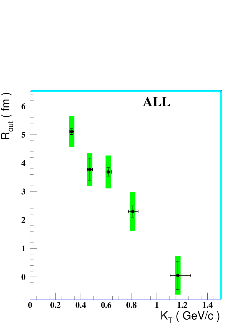
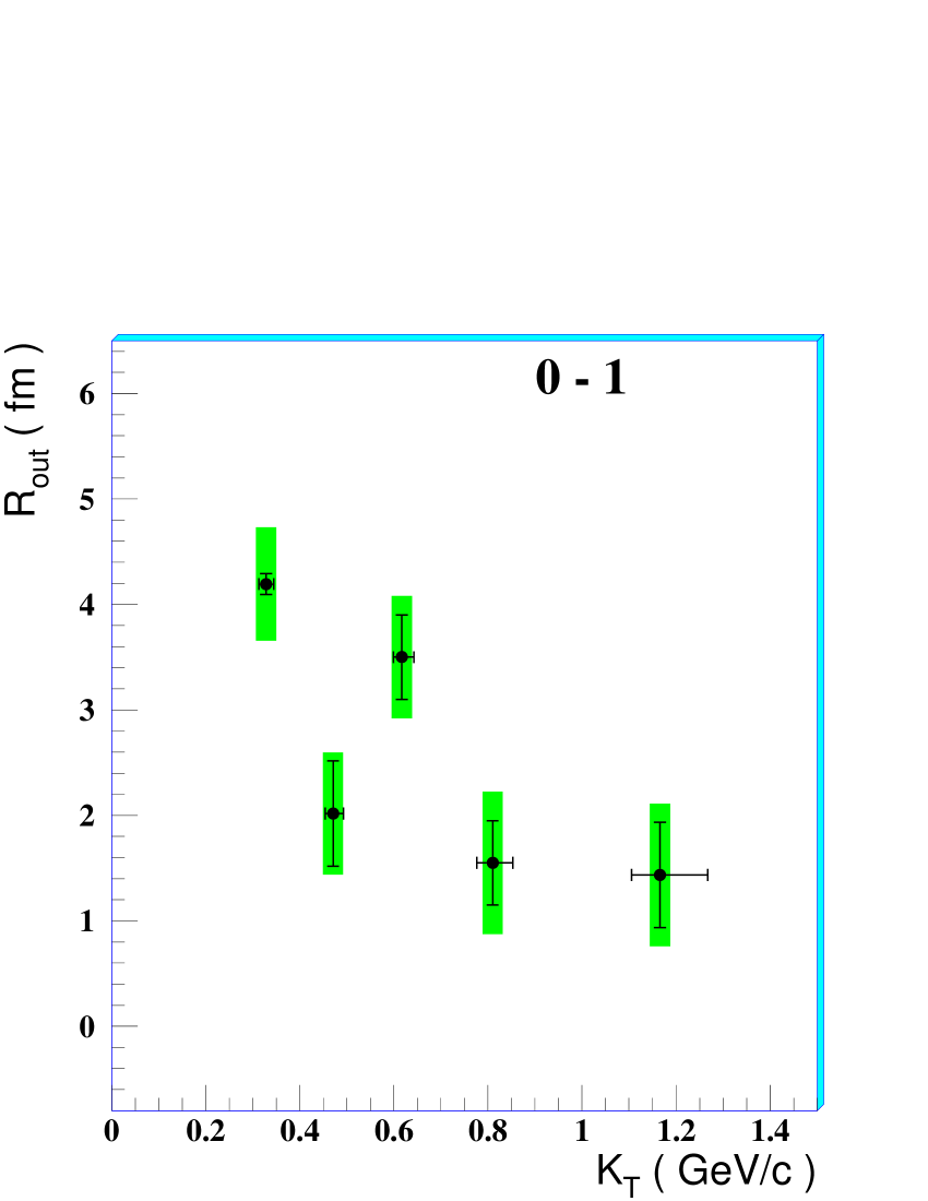
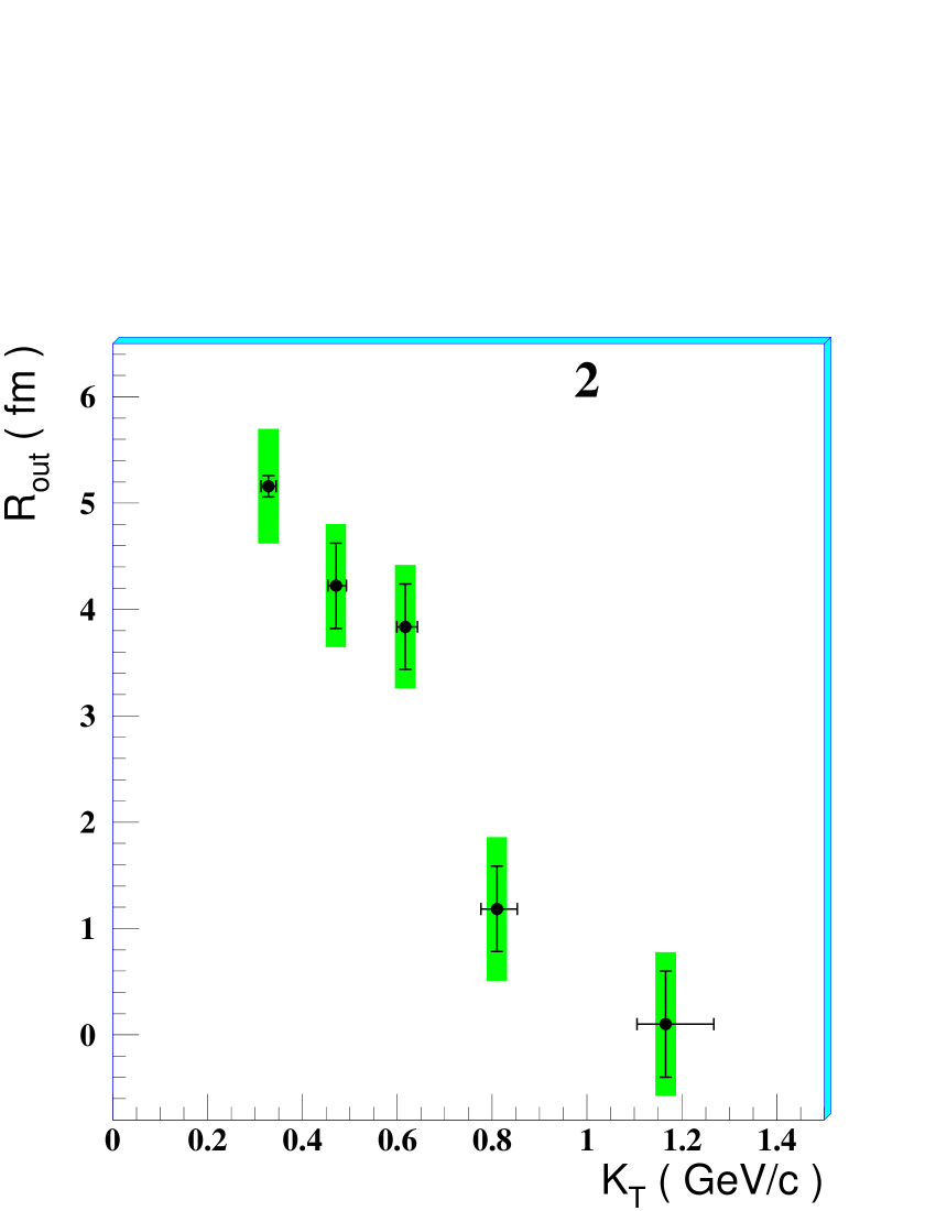
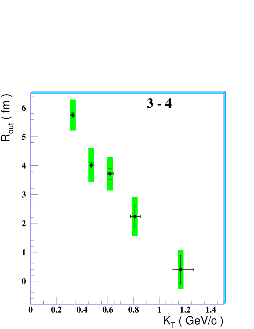
We found that the ratio $R_{\tt out}/R_{\tt side}$ is compatible with one in the explored $K_{\tt T}$ range (figure 15). Values smaller than unity for this ratio can be expected for sources with surface dominated emission [46], such as emission from an expanding shell. We plot the quantity $\frac{R_{\tt out}^{2}-R_{\tt side}^{2}}{\beta_{\rm T}^{2}}$ for the individual centrality classes in figure 15.

Figure 14: The ratio $R_{\tt out}/R_{\tt side}$ as a function of $K_{\tt T}$ for the data sample corresponding to the most central 53% of the Pb–Pb inelastic cross-section.

Figure 15: The ${\Delta\tau}^{2}$ parameter of equation 13 as a function of $K_{\tt T}$ for the three centrality classes. Statistical and systematic errors are indicated with line bars and shaded boxes (green on-line), respectively.

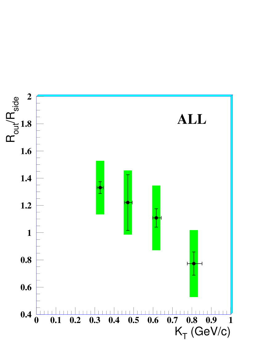
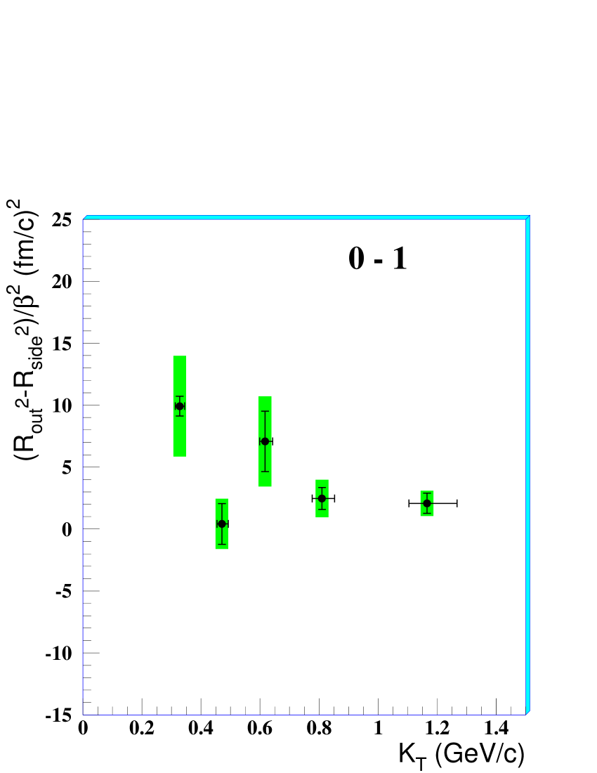
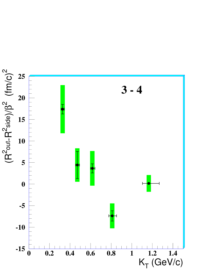
The data do not support the scenario of a long-lived source, but more likely that of a sudden freeze-out, $\Delta\tau$ being of the order of a few fm/$c$ for small $K_{\tt T}$ and nearly zero for high $K_{\tt T}$.

5.4 Consistency

In the first three rows of table 9 we have summarized the model parameters obtained from the study of $\tt h^{-}$ single-particle $m_{\tt T}$ spectra and two-particle correlation functions for the three centrality classes considered. These data provide implicitly a dynamical picture of the collision process.

To see if this picture is self-consistent, we can compare the two-dimensional rms width $R^{\rm freeze\,out}_{\rm rms}=\sqrt{2}R_{\rm G}$ with the two-dimensional rms width of a cold lead nucleus $R^{\rm Pb}_{\rm rms}=\sqrt{\frac{3}{5}}1.2A^{1/3}\simeq 4.5$ fm. For the most central collisions (class 3-4), the system expands by a factor $\approx$2 or, equivalently, by about 5 fm in the transverse direction. If the transverse flow velocity is equal to $\beta_{\perp}=\frac{3}{2}\langle\beta_{\perp}\rangle\simeq 0.67$ at the surface during the whole expansion, in a time of $\tau_{0}\simeq$ 7.5 fm/$c$ nuclear matter would travel over $\tau_{0}\beta_{\perp}\simeq$ 5 fm in the transverse direction. This is consistent with the previous estimate from the difference $R^{\rm freeze\,out}_{\rm rms}-R^{\rm Pb}_{\rm rms}$. Therefore, the dynamical description of the system expansion is internally consistent. Similar pictures can be drawn for the other two classes.

Coll.	$\sqrt{s_{\tt NN}}$	Centrality	$R_{\rm G}$ (fm)	$T$ (MeV)	$\langle\beta_{\perp}\rangle$	$\tau$ (fm/$c$)	$\Delta\tau$ (fm/c)
NA57	8.8	0 – 11 %	$6.6\pm 1.5$	$114^{+22}_{-14}$	$0.45_{-0.2}^{+0.1}$	$7.5\pm 0.7$
NA57	8.8	11 – 23 %	$6.9\pm 2.2$	$106^{+22}_{-13}$	$0.50_{-0.2}^{+0.1}$	$7.2\pm 0.6$	$1-2$
NA57	8.8	23 – 53 %	$4.3\pm 0.9$	$125^{+20}_{-13}$	$0.37_{-0.2}^{+0.1}$	$5.0\pm 0.5$
CERES	8.8	0 – 5 %	$12.1_{-2.6}^{+7.7}$	120	-	$6.6\pm 0.1$	-
CERES	8.8	5 – 10 %	$9.9_{-2.0}^{+5.2}$	120	-	$6.5\pm 0.1$	-
CERES	8.8	10 – 15 %	$10.1_{-2.2}^{+6.9}$	120	-	$6.3\pm 0.1$	-
CERES	8.8	15 – 30 %	$6.0_{-0.7}^{+1.1}$	120	-	$5.9\pm 0.1$	-
CERES	12.3	0 – 5 %	$7.2_{-0.6}^{+0.8}$	120	$0.58_{-0.06}^{+0.07}$	$7.3\pm 0.1$	-
CERES	12.3	5 – 10 %	$6.2_{-0.4}^{+0.5}$	120	$0.50_{-0.06}^{+0.06}$	$7.3\pm 0.1$	-
CERES	12.3	10 – 15 %	$5.9_{-0.4}^{+0.6}$	120	$0.50_{-0.07}^{+0.07}$	$7.0\pm 0.1$	-
CERES	12.3	15 – 30 %	$5.3_{-1.0}^{+0.7}$	120	$0.46_{-0.14}^{+0.13}$	$6.5\pm 0.2$	-
CERES	17.3	0 – 5 %	$6.9_{-0.3}^{+0.3}$	120	$0.49_{-0.06}^{+0.06}$	$8.2\pm 0.1$
CERES	17.3	5 – 10 %	$5.9_{-0.2}^{+0.3}$	120	$0.53_{-0.05}^{+0.06}$	$7.9\pm 0.1$	$2-3$
CERES	17.3	10 – 15 %	$5.9_{-0.4}^{+0.4}$	120	$0.46_{-0.04}^{+0.04}$	$7.5\pm 0.1$
CERES	17.3	15 – 30 %	$5.5_{-0.4}^{+0.4}$	120	$0.55_{-0.03}^{+0.03}$	$7.3\pm 0.1$
WA97	17.3	0 – 5%	$5.1\pm 0.6$	$120_{-11}^{+15}$	$0.46_{-0.10}^{+0.07}$	$5.6\pm 0.2$
WA97	17.3	5 – 12%	$5.0\pm 0.6$	$117_{-11}^{+16}$	$0.48_{-0.11}^{+0.08}$	$5.6\pm 0.2$	$\approx 0$
WA97	17.3	12 – 25%	$4.6\pm 0.4$	$121_{-11}^{+15}$	$0.47_{-0.10}^{+0.07}$	$5.1\pm 0.2$
WA97	17.3	25 – 40%	$3.2\pm 0.3$	$140_{-13}^{+26}$	$0.30_{-0.16}^{+0.09}$	$3.7\pm 0.2$
NA49	17.3	0 – 3%	$6.5\pm 0.5$	$120\pm 12$	$0.55\pm 0.12$	8	$3-4$
PHENIX	130	0 - 30%	$8.1\pm 0.3$	$125$	$0.51$	-
STAR	200	0 - 5%	$13.3\pm 0.2$	$97\pm 2$	$0.59\pm 0.05$	$9.0\pm 0.3$	$2.83\pm 0.19$
STAR	200	5 - 10%	$12.6\pm 0.2$	$98\pm 2$	$0.58\pm 0.05$	$8.7\pm 0.2$	$2.45\pm 0.17$
STAR	200	10 - 20%	$11.5\pm 0.2$	$98\pm 3$	$0.56\pm 0.06$	$8.1\pm 0.2$	$2.35\pm 0.16$
STAR	200	20 - 30%	$10.5\pm 0.1$	$100\pm 2$	$0.54\pm 0.06$	$7.2\pm 0.1$	$2.10\pm 0.09$
STAR	200	30 - 50%	$8.8\pm 0.1$	$108\pm 2$	$0.51\pm 0.06$	$5.9\pm 0.1$	$1.74\pm 0.12$
STAR	200	50 - 80%	$6.5\pm 0.1$	$113\pm 2$	$0.41\pm 0.06$	$4.0\pm 0.2$	$1.73\pm 0.10$

Table 9: Freeze-out parameters from HBT measurements in heavy ion collisions at SPS and RHIC. In the CERES [21] and PHENIX [38] analyses the freeze-out temperature has been fixed to the quoted values. The reported values of $\langle\beta_{\perp}\rangle$ for the PHENIX results have been computed from their parameterization of the transverse flow, which is assumed to be linear in the rapidity profile. In the STAR analysis [23], the values of $\langle\beta_{\perp}\rangle$ and $T$ have been extracted from blast-wave fits to pion, kaon, and proton transverse momentum spectra [54] and used to describe HBT radii.

6 Comparison with other experiments

In figure 16 we show HBT radii versus $K_{\tt T}$ measured in central Pb–Pb collisions at 40 $A$ GeV/$c$ by various experiments.

Figure 16: The HBT radii as a function of $K_{\tt T}$ in Pb–Pb collisions at 40 $A$ GeV/$c$ beam momentum. The CERES data set [21] corresponds to the most central 5% of the inelastic Au–Pb cross-section; those of NA49 [47] and NA57 correspond to the most central 7.2% and 11% of the inelastic Pb–Pb cross-section, respectively.

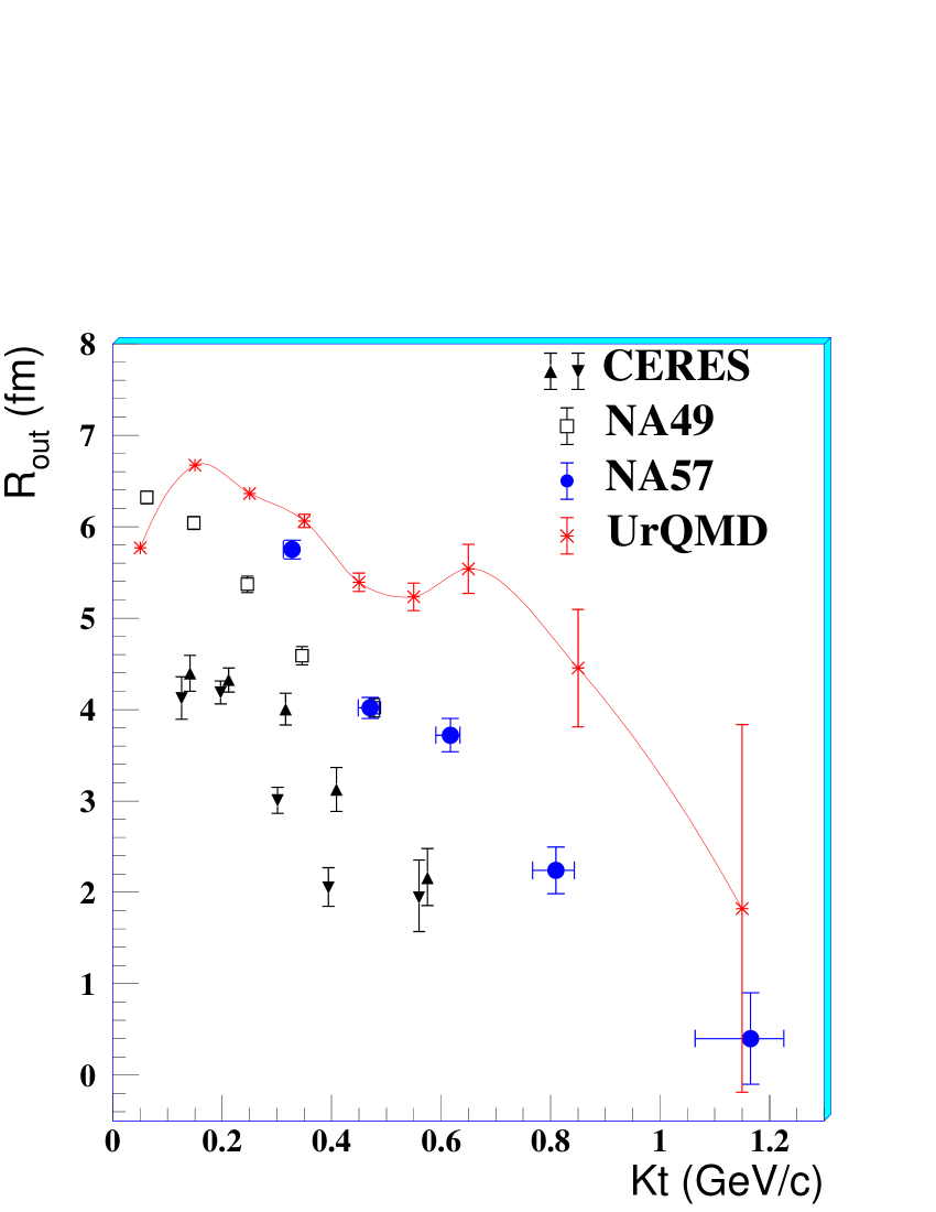
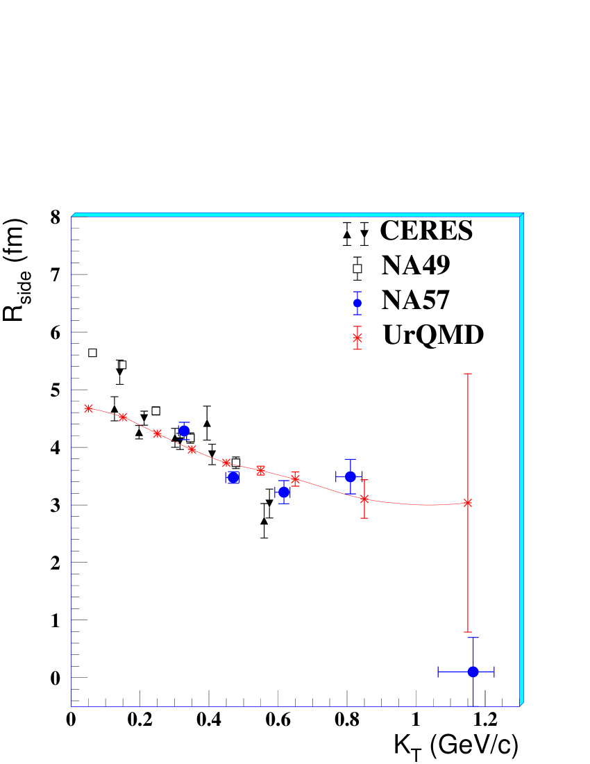
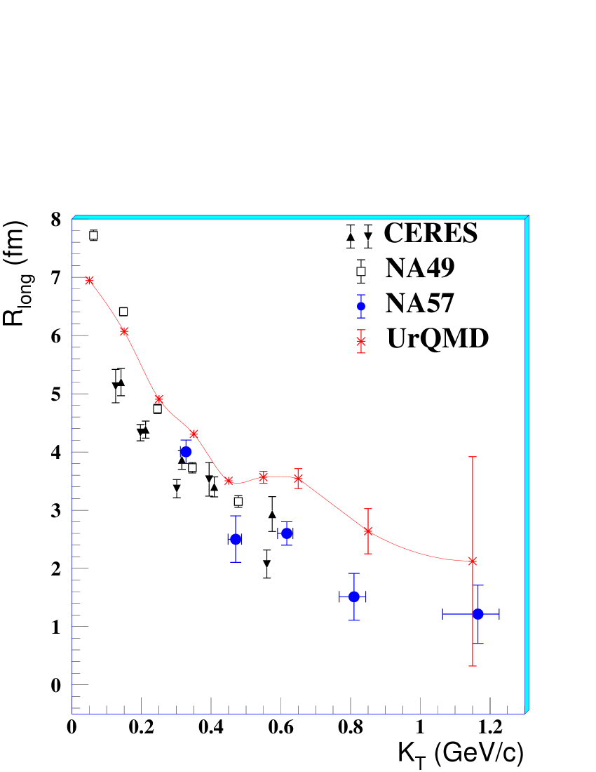
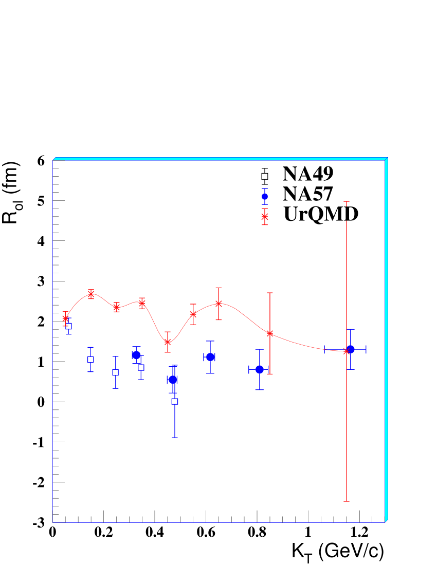
The overall agreement of the data is good for the $R_{\tt side}$ and $R_{\tt long}$ radii. A discrepancy is observed for the $R_{\tt out}$ radius, with the CERES results significantly smaller than the others. The values of the parameter $R_{\tt ol}$ depend strongly on the pair rapidity, hence a comparison with the CERES data, which are given at slightly backward rapidity, would not be straightforward. On the other hand, the agreement between NA49 and NA57 data, both shown at slightly forward rapidity over a similar rapidity range, is satisfactory also for the $R_{\tt ol}$ parameter. NA57 is the sole experiment that explores the high $K_{\tt T}$ region and our data suggest that the HBT radii $R_{\tt side}$, $R_{\tt out}$ and $R_{\tt long}$ decrease steadily up to $K_{\tt T}\approx 1.2$ GeV/$c$.

Superimposed on the experimental data, we show in figure 16 (with asterisks, connected by lines) results by Qingfeng Li et al. [48] based on the UrQMD v2.2 transport model [49]. The radii $R_{\tt long}$ and $R_{\tt side}$ are reasonably well in line with experimental data; the predicted $R_{\tt out}$ values are larger than those of the experimental data. As a consequence, the extracted quantity $\sqrt{R_{\tt out}^{2}-R_{\tt side}^{2}}$ of the pion emission source (see equation 13) becomes larger than the experimental evaluation.

In figure 17 we show the plot of the Yano-Koonin rapidity versus the pair rapidity, both evaluated in the centre-of-mass rest frame, as measured at different energies.

Figure 17: The Yano-Koonin rapidity plotted as a function of the pair rapidity for central Pb(Au)–Pb(Au) over a broad range of energies (open symbols are for $\mathrm{\pi^{-}}$–$\mathrm{\pi^{-}}$, closed symbols for $\mathrm{\pi^{+}}$–$\mathrm{\pi^{+}}$). Both quantities are in the center of mass frame of the colliding system. Data of other experiments are taken from references [50, 16, 17, 22].

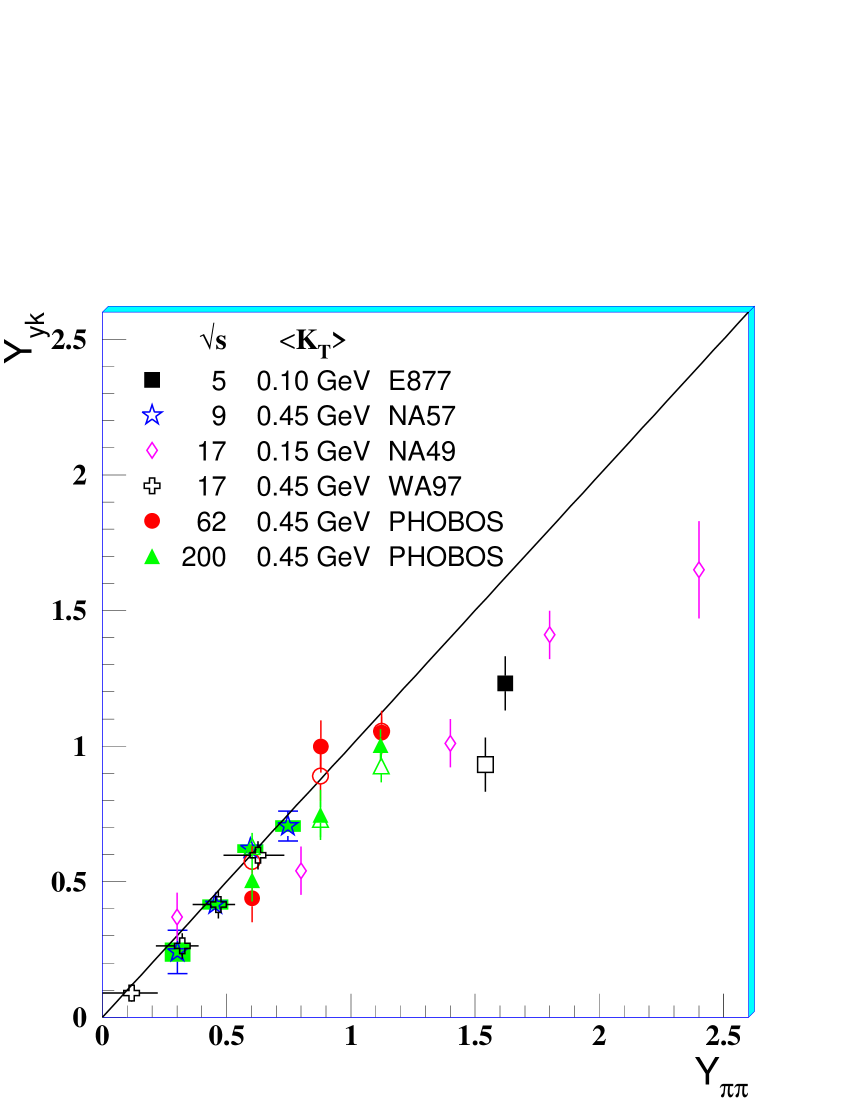
Figure 17 reveals a roughly universal dependence of $Y_{\rm yk}$ on $Y_{\pi\pi}$ for pions from central collisions, depending weakly, if at all, on $\sqrt{s_{\rm NN}}$. This trend is particularly striking given the very different centre-of-mass projectile rapidities ($\approx$ 1.57 and 5.5 for $\sqrt{s_{\rm NN}}$ = 5 and 200 GeV, respectively) and the corresponding widths of the pion distributions ${\rm d}N/{\rm d}y$.

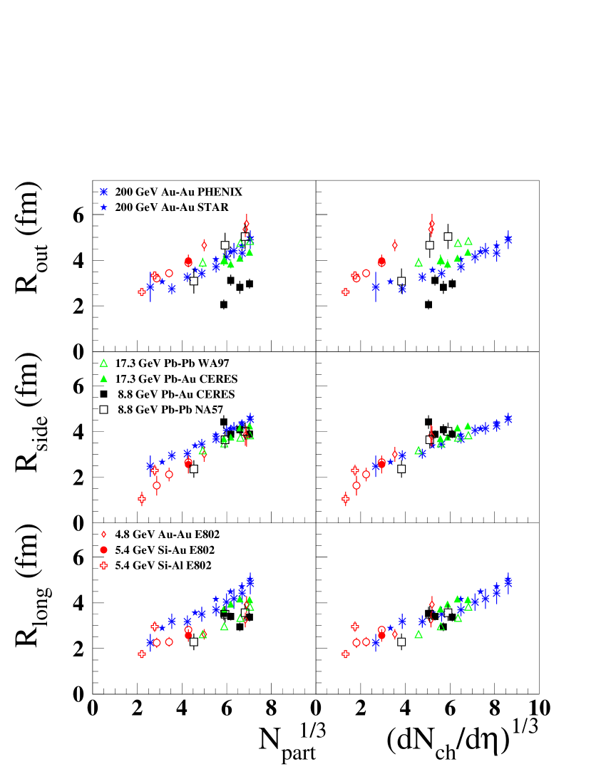
The centrality dependence of HBT radii is shown in figure 18 for a wide range of collision energies. The left panels show the dependence on the number of participating nucleons, $N_{\rm part}$. All of the radii exhibit a linear scaling in $N_{\rm part}^{1/3}$. Only the slope of the $R_{\tt long}$ dependence shows a significant increase from the AGS to RHIC, consistent with a lifetime that increases with both centrality and $\sqrt{s_{\rm NN}}$. The trend of increasing $R_{\tt long}$ with increasing $\sqrt{s_{\rm NN}}$ is reversed for $\sqrt{s_{\rm NN}}<$ 5 GeV [52]. We note that $R_{\tt out}$ radii from CERES at 40 $A$ GeV/$c$ are well below the observed systematics.

The right panels of figure 18 show the same radii as a function of $({\rm d}N_{\rm ch}/{\rm d}\eta)^{1/3}$. The primary motivation for exploring the $({\rm d}N_{\rm ch}/{\rm d}\eta)^{1/3}$ dependence is its relation to the final state geometry through the density at freeze-out. However, the two scaling quantities are highly correlated. In fact, the values of ${\rm d}N_{\rm ch}/{\rm d}\eta$ shown on the right side of figure 18 are derived (as suggested in reference [10]) from $N_{\rm part}$ using the $N_{\rm part}^{\alpha}$ parameterizations given in [53], and conversely, the $N_{\rm part}$ values are often calculated from multiplicity distributions using a Glauber model. Given this caveat, the $R_{\tt side}$ and $R_{\tt long}$ values exhibit a linear dependence on $({\rm d}N_{\rm ch}/{\rm d}\eta)^{1/3}$. The similar behaviour from $\sqrt{s_{\rm NN}}$ of 5 to 200 GeV leads one to believe that the approximate $N_{\rm part}$ scaling (initial overlap geometry) is a result of the scaling with multiplicity (final freeze-out geometry) and not the other way around.

Figure 18: The HBT radius dependence on number of participants (left) and on charged particle multiplicity (right). Data are for Pb(Au)–Pb(Au) collisions at several values of $\sqrt{s_{\rm NN}}$, and also for Si–A collisions at the lowest energy. Average transverse momentum $\langle K_{\rm T}\rangle$ is $\sim$450 MeV/$c$ for the PHENIX data [38] and $\sim$390 MeV/$c$ for the others [51, 21, 17, 23]. Open symbols are for $\mathrm{\pi^{-}}$–$\mathrm{\pi^{-}}$, closed symbols for $\mathrm{\pi^{+}}$–$\mathrm{\pi^{+}}$, but for the STAR, PHENIX and CERES results which combine the two sets. Systematic and statistical errors have been added when both available.

In table 9 we present, along with our results, a compilation of results on the source parameters obtained at the SPS and RHIC from blast-wave fits to HBT correlation functions. At all collision energies it is observed that, with increasing centrality: (i) the geometrical transverse dimension of the system at freeze-out, the average transverse flow, the proper time of the freeze-out and the duration of pion emission increase; (ii) the thermal freeze-out temperature decreases.

With increasing $\sqrt{s_{\rm NN}}$, both the proper time of the freeze-out (which can be assumed as the duration of the expansion) and the average transverse flow velocity increase, thus resulting in a stronger increase of the transverse radius parameter $R_{\rm G}$ at the freeze-out: after a faster expansion which lasts longer, the system ends up showing much larger spatial extent. The freeze-out temperature at top RHIC energy is also significantly smaller than that measured at SPS for a given collision centrality. This can be explained again as due to a longer and faster expansion, which causes the system to cool down more effectively. On the other hand, similar freeze-out emission durations of a few fm/$c$ are observed independently of the collision energy.

7 Conclusions

The analyses of transverse mass spectra of negatively charged hadrons and of Hanbury-Brown and Twiss correlation functions have provided a description of the later stages of the expansion dynamics of the system formed in Pb–Pb collisions at 40 $A$ GeV/$c$. They have been performed over a centrality range corresponding to the most central 53% of the inelastic Pb–Pb cross section.

Based on a model derived from hydro-dynamics, we have determined parameters describing the spatial dimension and the dynamical/thermal state of the system, namely the transverse radius and the temperature of the fireball at kinetic freeze-out, the average velocity of the collective flow in the transverse direction, the proper time of the freeze-out and the mean duration of particle emission. For central collisions, the system undergoes a strong collective expansion in the transverse directions, with an average velocity of about 45% of the speed of light, which lasts for about 7 fm/$c$. After this expansion, the system has doubled its transverse size and it freezes out at a temperature of about 110 MeV. For less central collisions, the expansion proceeds on a smaller scale; the higher temperature at freeze-out may be interpreted as the remnant of an earlier decoupling of the expanding system.

Concerning the time evolution, we have deduced that $\tt h^{-}$ emission is a fast process ($\Delta\tau\approx 1-2$ fm/$c$) starting after $∼$7.5 fm/$c$ (5 fm/$c$) in the case of central (semi-peripheral) collisions, that takes places in the bulk (i.e. it is not surface dominated). This resembles the decoupling process of photons in the early universe.

In the longitudinal direction, the indications are that particles emitted at a given rapidity are produced by source elements moving collectively at the same rapidity.

The kinetic freeze-out conditions for $\tt h^{-}$, namely temperature and transverse flow, are compatible with those obtained, within the same model, by studying the $m_{\tt T}$ spectra of singly-strange particles ($\mathrm{K^{0}_{S}}$, $\mathrm{\Lambda}$ and $\mathrm{\overline{\Lambda}}$) [3].

Quite universal kinetic freeze-out conditions are observed with increasing $\sqrt{s_{\rm NN}}$ from SPS to RHIC, with moderate increases (by less than 20%) of the transverse flow velocity and of the duration of the expansion. The latter effect is consistent with the lower (by $\approx$20%) freeze-out temperatures measured at top RHIC energy ($\sqrt{s_{\rm NN}}=200$ GeV); on the other hand, the combined effect of a faster and longer expansion causes the final transverse size at freeze-out to be significantly larger (about a factor of two for central collisions) at top RHIC energy than at SPS.

References

- [1] Karsch F 2002 Lect. Notes Phys. 583 209
- [2] Ritter H G and Wang X-N (ed) 2004 J. Phys. G: Nucl. Phys.30 S633-S1430 (Proc. Quark Matter 2004) Csörgo T, Dávid G, Lévai P and Papp G (ed) 2006 Nucl. Phys.A 774 1-968 (Proc. Quark Matter 2005)
- [3] Antinori F et al. (NA57 Collaboration) 2006 J. Phys. G: Nucl. Phys.32 xxx-yyy
- [4] Schnedermann E, Sollfrank J and Heinz U 1993 Phys. Rev.C 48 2462 Schnedermann E and Heinz U 1994 Phys. Rev.C 50 1675
- [5] Hanbury-Brown R and Twiss R Q 1954 Phil. Mag. 45 633 Goldhaber G, Goldhaber S, Lee W and Pais A 1960 Phys. Rev.178 300
- [6] Antinori F et al. (NA57 Collaboration) 2006 J. Phys. G: Nucl. Phys.32 427-441
- [7] Antinori F et al. (NA57 Collaboration) 2004 J. Phys. G: Nucl. Phys.30 823-840
- [8] Manzari V et al. 1999 J. Phys. G: Nucl. Phys.25 473 Manzari V et al. 1999 Nucl. Phys.A 661 761c
- [9] Antinori F et al. (NA57 Collaboration) 2005 J. Phys. G: Nucl. Phys.31 321-335
- [10] Lisa M, Pratt S, Soltz R and Wiedemann U A 2005 Ann. Rev. Nucl. Part. Sci. 55 357-402, nucl-ex/0505014
- [11] Tomasik B and Wiedemann U A 2003 in Quark Gluon Plasma 3, Hwa R C and Wang X N (ed) World Scientific, hep-ph/0210250
- [12] Hirano T 2004 J. Phys. G: Nucl. Phys.30 S845-S851 Torrieri G and Rafelski J J. Phys. G: Nucl. Phys.30 S557-S564 Heinz U W 2005 J. Phys. G: Nucl. Phys.31 S717-S724 Csernai L P, Molnár E, Nyíri Á and Tamosiunas K 2005 J. Phys. G: Nucl. Phys.31 S951-S957 Steinberg P A 2005 Nucl. Phys.A 752 423c-432c
- [13] Afanasiev S V et al. 2002 Phys. Rev.C 66 054902 Anticic T et al. 2004 Phys. Rev.C 69 024902
- [14] Afanasiev S V et al(NA49 Collaboration) 2003 Phys. Lett.B 557 157-166
- [15] Bamberger A et al(NA35 Collaboration) 1988 Phys. Lett.B 203 320-326 Bamberger A et al(NA35 Collaboration) 1988 Z. Phys.C 38 79 Alber T et al(NA35 Collaboration) 1995 Z. Phys.C 66 77 Alber T et al(NA35 Collaboration) 1995 Phys. Rev. Lett.74 1303
- [16] Appelshäuser H et al. (NA49 Collaboration) 1998 The Eur. Phys. J. C 2 661
- [17] Antinori F et al. (WA97 Collaboration) 2001 J. Phys. G: Nucl. Phys.27 2325-2344
- [18] Boal D, Gelbke C K and Jennings B K 1990 Rev. Mod. Phys. 62 553
-
[19]
Brun R, Bruyant F, Maire M, McPherson A C and Zanarini P 1985 GEANT3 User Guide
CERN Data Handling Division, DD/EE/84-1,
http://wwwinfo.cern.ch/asdoc/geantold/GEANTMAIN.html Brun R et al 1994 GEANT Detector Description and Simulation Tool CERN Program Library Long Write-up W5013 - [20] Bowler M G 1991 Phys. Lett.B 270 69 Sinyukov Yu M et al. 1998 Phys. Lett.B 432 249
- [21] Adamova D et al(CERES Collaboration) 2003 Nucl. Phys.A 714 124
- [22] Back B B et al(Phobos Collaboration) 2006 Phys. Rev.C 73 031901
- [23] Adams J et al(STAR Collaboration) 2005 Phys. Rev.C 71 044906
- [24] Gamow G 1928 Z. Phys.51 204 Gurney R W and Condon E U 1929 Phys. Rev.33 (1929) 204
- [25] Gyulassy M, Kauffmann S K and Wilson L W 1979 Phys. Rev.C 20 2267
- [26] Koonin S E 1977 Phys. Lett.B 70 43 Pratt S et al1994 Nucl. Phys.A 566 103c
- [27] Bjorken J D 1983 Phys. Rev.D 27 140
- [28] U. Heinz U, Hummel A, Lisa M A and Wiedemann U A 2002 Phys. Rev.C 66 044903
- [29] Yano F and Koonin S 1978 Phys. Lett.B 78 556 Podgoretskii M I 1983 Sov. J. Nucl. Phys. 37 272
- [30] Heinz U, Jacak B V 1999 Ann. Rev. Nucl. Part. Sci. 49 529-579
- [31] Heinz U, Tomášik B, Wiedemann U A and Wu Y -F 1996 Phys. Lett.B 382 181
- [32] Wu Y-F, Heinz U, Tomášik B and Wiedemann U A 1998 Eur. Phys. J C 1 599
- [33] Chapman S, Rayford Nix J and Heinz U 1995 Phys. Rev.C 52 2694
- [34] Sinyukov Yu M 1995 Hot Hadronic Matter: Theory and Experiment (New York: Plenum)
- [35] Adams J. et al(STAR Collaboration) 2004 Phys. Rev. Lett.92 182301
- [36] Adcox K et al(PHENIX Collaboration) 2004 Phys. Rev.C 69 024904
- [37] Arsene I et al(BRHAMS Collaboration) 2005 Phys. Rev.C 72 014908
- [38] Adler S S et al(PHENIX Collaboration) 2004 Phys. Rev. Lett.93 152302
- [39] Makhlin N and Sinyukov Yu M 1988 Z. Phys.C 39 69 Akkelin S V and Sinyukov Yu M 1995 Phys. Lett.B 356 525
- [40] Bertsch G 1989 Nucl. Phys.A 498 173c
- [41] Pratt S 1986 Phys. Rev.D 33 1314
- [42] Bertsch G, Gong M and Tohyama M 1988 Phys. Rev.C 37 1896
- [43] Bertsch G and Brown G E 1989 Phys. Rev.C 40 1830
- [44] Rischke D 1996 Nucl. Phys.A 610 88
- [45] Rischke D and Gyulassy M 1996 Nucl. Phys.A 608 479
- [46] Heiselberg H and Vischer A P 1998 Eur. Phys. J. C 2 593
- [47] Kniege S et al(NA49 Collaboration) 2006 AIP Conference Proceedings 828; nucl-ex/0601024 Kniege S et al(NA49 Collaboration) 2004 J. Phys. G: Nucl. Phys.30 S1073-S1078
- [48] Qingfeng Li, Bleicher M and Stöcker H 2006 Phys. Rev.C 73 064908 Qingfeng Li 2006 private communication
- [49] Bass S A et al(UrQMD-Collaboration) 1998 Prog. Part. Nucl. Phys. 41 255 Bleicher M et al(UrQMD-Collaboration) 1999 J. Phys. G: Nucl. Phys.25 1859 Bratkovskaya E L, Bleicher M, Reiter M, Soff S, Stöcker H, van Leeuwen M, Bass S A and Cassing W 2004 Phys. Rev.C 69 054907Zhu X, Bleicher M and Stöcker H 2005 Phys. Rev.C 72 064911
- [50] Miskowiec D et al(E877 Collaboration) 1996 Nucl. Phys.A 610 C227
- [51] Ahle L 2002 et al(E802 Collaboration) Phys. Rev.C 66 054906
- [52] Lisa M A et al(E895 Collaboration) 2000 Phys. Rev. Lett.84 2798
- [53] Adler S S et al(PHENIX Collaboration) 2005 Phys. Rev.C 71 034908
- [54] Adams J et al(STAR Collaboration) 2004 Phys. Rev. Lett.92 112301