^aDAPNIA/SPhN, CEA/Saclay, F-91191 Gif-sur-Yvette Cedex, France
^bGSI, Planckstrasse 1, D-64291 Darmstadt, Germany
^cIPN Orsay, BP 1, F-91406 Orsay Cedex, France
^dUniversity of Santiago de Compostela, 15706 Santiago de Compostela, Spain
^eCEN Bordeaux-Gradignan, UMR 5797 CNRS/IN2P3 - Université Bordeaux 1, BP 120, F-33175, Gradignan, France
^fCalifornia Institute of Technology, Pasadena, CA 91125 USA
^gJet Propulsion Laboratory,California Institute of Technology, Pasadena, CA 91109 USA
^hUniversity of New Hampshire, Durham, NH 03824, USA
ⁱTU Munich, 85747 Garching, Germany
^jArgonne National Laboratory, Argonne, IL 60439-4083 USA
^kCENPA/University of Washington, Seattle WA 98195 USA

Abstract - The spallation residues produced in the bombardment of ${}^{56}Fe$ at 1.5, 1.0, 0.75, 0.5 and 0.3 A GeV on a liquid-hydrogen target have been measured using the reverse kinematics technique and the Fragment Separator at GSI (Darmstadt). This technique has permitted the full identification in charge and mass of all isotopes produced with cross-sections larger than $10^{-2}$ mb down to $Z=8$. Their individual production cross-sections and recoil velocities at the five energies are presented. Production cross-sections are compared to previously existing data and to empirical parametric formulas, often used in cosmic-ray astrophysics. The experimental data are also extensively compared to different combinations of intra-nuclear cascade and de-excitation models. It is shown that the yields of the lightest isotopes cannot be accounted for by standard evaporation models. The GEMINI model, which includes an asymmetric fission decay mode, gives an overall good agreement with the data. These experimental data can be directly used for the estimation of composition modifications and damages in materials containing iron in spallation sources. They are also useful for improving high precision cosmic-ray measurements.

I Introduction

The spallation cross-sections of nuclides such as Fe have been historically studied to understand the propagation of cosmic-ray ions in the Galaxy, and to determine the composition of the Galactic Cosmic Ray (GCR) source Tsao93 - Zeit . Galactic cosmic rays constitute a superthermal gas that is partially confined in the Galaxy by interstellar magnetic fields with some leakage into the intergalactic medium. While propagating in the Galaxy, cosmic rays pass through the interstellar medium and some primary cosmic ray nuclei spallate into secondary cosmic ray nuclei. As measured by instruments in the solar system, the composition includes both primary cosmic rays whose abundance is depleted by spallation, and secondary cosmic rays produced by spallation. As a result of spallation during propagation, certain elements in the GCRs are far more abundant (often by orders of magnitude) than in solar system material. Examples of these ”secondary elements” include Li, Be, B which are mainly spallation products of C and O, and Sc, Ti, V and Cr which are mainly spallation products of Fe. Conversely, those elements where the abundance of heavier elements is much smaller, and hence have very small secondary contributions are ”primary elements.” Prominent examples include C and O and Fe. Provided the spallation cross-sections are known, the abundance of secondary elements relative to primary elements are a measure of the amount of material cosmic rays traverse in the Galaxy. This in turn constrains astrophysical models of cosmic rays in the Galaxy. It is possible to correct abundance measurements for propagation back to the ”source,” that is, to determine the composition of the material that became the cosmic rays. The secondary-to-primary ratios combined with the cross-sections determine the amount of material traversed during propagation in the Galaxy; the amount of material traversed, again with the cross-sections, is then used to correct the measured abundances to the source abundances. Thus, uncertainties in the cross-sections are more significant than any details of the astrophysical models. (The exception to this generalization are the unstable secondaries.) In recent years, new high resolution elemental and isotopic measurements have become available (i.e. the ACE ACE and Ulysses Ulysses space missions), including measurements in the iron region. The main source of uncertainties in determining both cosmic-ray secondary production and source composition using these data are uncertainties in the nuclear cross-sections. The interstellar medium is composed $\sim 90\%$ by number of H atoms and ions. Most high resolution measurements are of cosmic rays with energies per nucleon in the interstellar medium of $\sim 0.5$ to $\sim 1.5$ GeV. The cross sections reported here are thus directly applicable to improved interpretation of high-precision cosmic-ray measurements.

Spallation reactions have also gained a renewed interest with the recent projects of spallation neutron sources and accelerator-driven sub-critical reactors systems considered for the transmutation of nuclear waste (Accelerator Driven Systems (ADS)). In these systems, a high-intensity proton beam of energy around 1 GeV is guided on a spallation target made of a high-mass material. In ADS, neutrons produced in the spallation target are used to maintain the reactivity in the sub-critical reactor where nuclear waste can be transmuted. The proton beam under vacuum in the accelerator has generally to cross a window before entering the spallation target. As it is continuously submitted to the proton beam irradiation, it is one of the most sensitive parts in ADS or spallation-neutron-source design. Among the problems created by the proton irradiation are the changes in the chemical composition of the window material and embrittlement created by gas production and atomic displacements (DPA) in the crystal lattice. A large range of materials have been studied for this window and, in most of the projects, martensitic steels composed at 90 % of Iron (with also substantial quantities of Chromium and Molibdenium) have been retained due to their resistance to thermal constraints and radiation effects. Therefore, it is important to have a good knowledge of the production cross-sections of spallation residues in Iron and of their recoil velocity.

In recent years, an important effort has been undertaken, mainly under the framework of the HINDAS European project HINDAS , to collect a comprehensive set of high-quality spallation data regarding the production of neutrons sylvie ; NESSI , light charged particles NESSI2 and residual nuclei. The general goal is to better understand the reaction mechanisms in order to improve the models that are then implemented into high-energy transport codes. These codes, validated on experimental data, can afterwards be used to reliably predict all quantities needed for the design of ADS or spallation sources as neutron production, activation or damages.

As concerns residue production, up to now the emphasis was put on spallation reactions on heavy nuclei. Isotopic cross-sections of residues produced in the reactions ${}^{197}Au+p$ Fanny ; Pepe at 800 A MeV , ${}^{208}Pb+p$ at 1 A GeV and 500 A MeV Wla ; Timo ; Bea ; Laurent , ${}^{238}U+p$ at 1 A GeV Julian ; Monique , ${}^{238}U+d$ at 1 A GeV  Quique ; Jorge have already been measured using the reverse-kinematics method at GSI (Darmstadt). In this paper we present new experimental results concerning the isotopic production cross-sections and recoil velocities of spallation residues in the reaction ${}^{56}Fe+p$ for five energies of the iron beam (0.3, 0.5, 0.75, 1.0 and 1.5 A GeV). This measurement is the first consistent set of data on isotopically identified residues on a large energy domain and for a light nucleus of practical interest. The comparison of the obtained data with various models, some of them being quite successful for heavy systems, allows testing their predicting capabilities for light nuclei and their dependence on beam energy.

II Experimental method

II.1 Experimental set-up

In October 2000, an experiment was performed using the reverse kinematics at GSI in Darmstadt, Germany. A primary beam of ${}^{56}Fe$ was delivered by the heavy-ion synchrotron SIS at energies of 0.3, 0.5, 0.75, 1.0 and 1.5 A GeV and directed onto a liquid-hydrogen target designed and built in the Laboratoire National Saturne (Saclay, France) Chesny .

The liquid-hydrogen thickness was $87.3mg/cm^{2}$ contained by titanium windows of $20\mu m$ each. Two additional Ti foils were used to isolate the vacuum around the target from the vacuum of the beam pipe for security reasons so that a total of $36mg/cm^{2}$ of Ti contributes to the empty-target counting. Measurements were repeated with an identical empty target in order to subtract the production on the titanium container from the measured yields of residual nuclei. The contribution of these walls to the counting rates was below 10 % for the main part of the residues and below 20 % for the lightest ones.

The time structure of the primary beam was a pulse of 6 s every 12 s, and the intensity was limited to $10^{7}$ part/spill. This beam intensity was measured using a secondary-electron emission monitor (SEETRAM) Jur02 calibrated at the beginning and at the end of each set of measurements at a given beam energy. This was done at low counting rates with a plastic scintillator as absolute reference.

Residual nuclei produced in the reaction with the target were focused in the beam direction and analyzed with the FRS (Fragment Separator) FRS operated as an achromatic magnetic spectrometer. Fig. 1 is a schematic diagram of the experimental setup showing the four large dipole magnets and the essential detector equipment.

Figure 1: Schematic layout of the FRS fragment spectrometer. Fragments are analyzed by the four large dipole magnets. Scintillators at S2 and S4 measure the time of flight over the second half of the spectrometer as well as the horizontal positions in the dispersive focal planes at S2 and at S4. The MUSIC detector (ionization chamber) gives information about the energy loss of the fragment. Multi-Wire Proportional Chambers (MWPC) are used for beam tuning and removed for production measurements.

Due to their relativistic energies, the fragments produced in this experiment are fully stripped. The horizontal positions of these ions and a time of flight (ToF) were measured with two plastic scintillators, one located in the intermediate dispersive plane S2 and the other one installed at the final achromatic focal plane S4. The signal from the scintillator at S4 was used as the trigger for the acquisition of all detectors. The nuclear charge Z was determined using a multiple-sampling ionization chamber (MUSIC). The energy loss in the gas produces a signal proportional to $\frac{Z^{2}}{\beta^{2}}$, allowing the determination of Z with a resolution of $\Delta Z=0.3$ (FWHM) charge units.

The knowledge of the horizontal positions of the ions determines precisely the radii $\rho 1$ and $\rho 2$ of their trajectories in the two magnetic sections of the spectrometer. An absolute calibration is obtained with the iron beam detected in specific measurements at low intensity. Together with the magnetic field strengths in the dipoles measured with Hall-effect probes, the magnetic rigidities $B\rho 1$ and $B\rho 2$ can be determined for each ion. Therefore, a total identification of the nature of the ions could be performed from the relation :

$$\frac{A}{Z}=\frac{eB\rho}{m_{u}c\beta\gamma}$$ (1)

where $m_{u}$ was the atomic mass unit and $\beta$ $\gamma$ were deduced from the experimental time of flight. Note that in this formula we have replaced the mass of the $(A,Z)$ ion by $A.m_{u}$ which means neglecting binding energies compare to nucleon masses.

The FRagment Separator has a momentum acceptance of $\pm 1.5$%. Therefore, about 18-20 different settings of the FRS were needed to cover the complete velocity distribution of all the ions. Figure 2 shows the complete fragment coverage in the Z vs. A/Z plane for 1 GeV per nucleon ${}^{56}Fe$ on the hydrogen target. The plot was made by adding histograms from individual settings, each one normalized to the dose of the primary beam. Fragments are well resolved and easily identifiable in this plot down to lithium. However, for the lightest elements the transmission of the spectrometer is very low, necessiting a dedicated method of analysis. This has been done only at 1 GeV per nucleon and reported in a separate paper  Paolo . Therefore, we show in this paper results of the production cross section and recoil velocity only down to Z=8-10, depending on the beam energy considered.

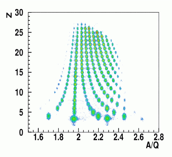
Figure 2: Complete isotope coverage in Z vs. A/Q (actually identical to A/Z) for 1 A GeV ${}^{56}Fe$ on the liquid-hydrogen target. The plot is built from data of overlapping settings, normalized to the primary beam intensity and superimposed.

II.2 Data analysis

The fragments are first identified in Z using the ionization chamber, taking into account the position and velocity dependence of the energy-loss signal. The velocity distribution of the fragments is obtained with high precision using the time-of-flight and magnetic-rigidity measurements. The experimental time-of-flight between the intermediate and the final focal plane is precise enough for an unambiguous identification of the fragment mass. After identification of the isotope, a more accurate value of the longitudinal velocity can be deduced from the magnetic rigidity in the first part of the spectrometer using relation 1.

Assuming that the reaction takes place at the center of the target, the fragment velocity is corrected for the energy loss in the target and transformed into the reference frame of the projectile at rest. A measurement of the recoil velocity of the fragments is thus obtained in that frame. To obtain the production cross-section of a given isotope, it is necessary to reconstruct the full velocity distribution by adding the partial ones measured in different settings, with the proper normalization. An example of the velocity distribution for ${}^{38}K$ is shown in Fig. 3. For this isotope, five different settings of the FRS were needed in order to reconstruct the complete velocity distribution.

Figure 3: Longitudinal velocity distribution of ${}^{38}K$ detected as a residual nucleus at 1 A GeV and expressed in the rest frame of the iron beam. Five different settings of the FRS were needed to reconstruct the complete distribution. The yield (here in arbitrary units) detected in each setting is normalised by the number of incident iron nuclei and corrected for the acquisition dead time.

Due to potential damages in the detectors, isotopes having a magnetic rigidity too close to the beam one could not be measured. This is why the detection of ${}^{54}Mn$ was not possible in this experiment. For the same reason, some settings of other isotopes could not be obtained, leading to truncated measured velocity distributions. In that case a fit by a Gaussian function excluding the truncated zones was used to reconstruct the full distribution and then determine the total cross-section, the mean value of the velocity and its variance. In the case of a truncated zone in the velocity distribution too large to have a converging fit, the parameters of the Gaussian were constrained using the neighboring isotopes. The reconstruction procedure leads to an uncertainty on both the velocity determination and the isotope production cross-section. These uncertainties have been estimated by taking into account the fluctuation of the reaction point in the target and by doing reasonable variations of the fitted parameters for several groups of isotopes.

II.3 Corrections and uncertainties

The isotopic production cross-section of each spallation residue $\sigma(Z,A)$ was obtained from the difference between the yield measured with the hydrogen target $(Y_{H}(Z,A))$ and the yield measured with the empty target $(Y_{e}(Z,A))$, each of them corrected for their dead time (correction factor $f_{\tau H}(f_{\tau e})$) and normalized to the number of incident iron nuclei $N_{Fe\ H}(N_{Fe\ e})$.

$$\sigma(Z,A)=\left(\frac{Y_{H}(Z,A)\cdot f_{\tau H}}{N_{Fe\ H}}-\frac{Y_{e}(Z,A)\cdot f_{\tau e}}{N_{Fe\ e}}\right)\cdot\frac{f_{\epsilon}\cdot f_{trans}\cdot f_{sec}}{N_{H}}$$ (2)

The cross section is finally obtained after a division by the number of hydrogen nuclei per surface unit $N_{H}$ and with additional corrections due to the detection efficiency ($f_{\epsilon}$), the transmission of the FRS ($f_{trans}$) and the secondary reactions ($f_{sec}$) estimated for hydrogen events. It was determined that, even at the lowest energy, a correction for possible change of charge state is not necessary.

Losses of events due to the dead time of the experiment, mainly due to the acquisition capability, are estimated for each run from the ratio between the free triggers measured on a scaler of high counting-rate capability and the number of recorded events (or accepted triggers). During the experiment, the counting-rate conditions were kept so that this correction never exceeded 30%, and was most frequently smaller for detection at magnetic rigidities substantially different from the beam rigidity.

An estimation of the global detection efficiency $f_{\epsilon}$ including the detailed analysis of all needed information can be obtained from the difference between the number of accepted triggers and the final number of events that have been analyzed. An event can be analyzed if all the elements required have been registered without any problem: position at the two focal planes, time of flight and energy loss in the MUSIC detector. The trigger signal obtained by a narrow coincidence on high signals produced by highly ionizing particles is here supposed to identify a true heavy ion with a probability of nearly 100%. In almost all settings this efficiency was in the range 96-99%.

Corrections due to secondary reactions in the target and in the layers of matter on the trajectory of the fragments (mainly the plastic scintillator of 3 mm thickness at S2) were calculated following the method described in pagkh as previously used in other similar experiments Fanny . If a second reaction occurs in the target, the initially produced ion becomes lighter, so that cross sections of light ions are artificially increased (and the one for the corresponding heavy ion decreased). If a reaction occurs in the plastic at S2, the spallation ion will most often be out of the narrow magnetic rigidity acceptance in the second part of FRS and so will be lost at S4. Total nuclear interaction cross sections for the different fragments were estimated using the parametric formula of Kox et al Kox . The maximum value (8%) of this correction factor is obtained for the secondary reactions in the target leading to the lightest evaporation residues. It decrease to zero for heavy residues. The correction due to the lost in the scintillator if a reaction occures is of the order of 3.5% and was taken into account (as a function of the nature of the ion and of it’s mean energy). The attenuation of the beam flux inside the finite target thickness was also taken into account in this correction and is equal to -2% for a reaction cross section of 700 mb.

The transmission correction is the most important factor concerning losses in the detection. Due to its geometrical characteristics and the ion optics, the FRS has only an angular acceptance of $15$ mrad around the beam axis, and a large number of the fragments analyzed in this experiment have an angular distribution at the entrance of the FRS larger than this acceptance. An evaluation of the fraction of the residual yield not detected in the experiment had to be made from the measured velocity distribution of the fragment as it is described in trans . Considering that, in the projectile reference frame, the emission of the fragments can be described as a 3-D Gaussian distribution around a mean longitudinal recoil, the width of the angular distribution in the laboratory frame can be obtained from the longitudinal velocity distribution measured in the experiment:

$$\sigma(\theta)\approx\frac{\sigma(v_{\parallel})}{<v_{\parallel}>}$$ (3)

where $<v_{\parallel}>$ is the mean value and $\sigma(v_{\parallel})$ the width of this distribution for evaporation residues of a given mass.

The transmission through the FRS can be parameterized as :

$$T=1-exp(-\frac{\alpha_{eff}(x2,x4)^{2}}{2\sigma(\theta)^{2}})$$ (4)

where $\alpha_{eff}(x2,x4)$ is the effective angular acceptance of the FRS as a function of the ion positions $x2$ and $x4$ respectively at the intermediate S2 and the final focal planes S4. This angle was calculated with the code described in reference trans using 15 mrad as the maximum angular acceptance when the ion optics is the most appropriate.

The transmission factor varies from 1 (no correction) to 0.4 for the lightest fragments that have a much larger angular distribution (see Fig. 4) for the three highest energies. Various reasonable assumptions on the calculation of $\alpha_{eff}(x2,x4)$ lead to uncertainty estimations on $T$ of $1\%$ to $15\%$ for the lightest evaporation residues. However, the analysis has revealed that at 500 and 300 MeV/A, the magnetic optics settings used during the experiment was not optimal and that the maximum acceptance of the FRS was reduced to $9.15$ mrad. This value has been taken into account in the transmission factor leading to much larger corrections for these two energies as it can be seen in Fig. 4.

For the absolute normalization, the precision on the target thickness has been studied in previous experiments  mustapha and is estimated to be $2.5\%$. The absolute numbers of incident ions $N_{Fe\ H}$ and $N_{Fe\ e}$ for runs with the hydrogen target and the empty target respectively are obtained from the SEETRAM calibration with an absolute error estimated to be $2.8\%$.

Experimental values for the isotopic cross-sections with their errors are listed in appendix A. The ${}^{54}Mn$ that could not be measured was obtained by a smooth interpolation between the neighboring isotopes so the value given in the tables is followed by (Interp.). This value is used to obtain integrated quantities as the mass or charge distributions and in the evaluation of the total reaction cross section also given in appendix A.

Final results of the mean recoil velocity and the width of the velocity distributions for the various residual nuclei are presented in appendix B. Errors quoted here are due to the velocity reconstruction procedure above described and to the magnetic-rigidity determination. In the case of a truncated velocity distribution, results partially interpolated are followed by (I). The minus sign means that the recoil velocity is opposite to the original direction of the iron beam or in other words in the direction of the proton motion in the iron at rest system.

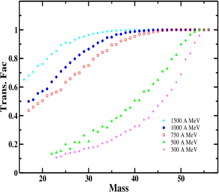
Figure 4: Transmission factor as a function of the mass number of the residue for the five energies presented in this work (see text).

III Results

III.1 Isotope production cross sections

Using the experimental method described above it was possible to measure at five different energies most of the residues produced in the spallation reaction of iron with cross-sections larger than $10^{-2}$ mb, from cobalt (Z=27) down to oxygen (Z=8) or neon (Z=10) depending on the energy. At 1 A GeV, cobalt isotopes have not been measured.

Figures 5, 6, 7, 8 and 9 show the isotopic distribution cross sections at the five beam energies. Error bars do not appear as they are smaller than the data points. The position of the maximum of these isotopic curves is correlated with the excitation energy transferred in the collision between the projectile and the target. In the case of a peripheral collision, in which the excitation energy is limited, only a few particles are evaporated by the fragment, leading to the population of isotopes close to stability. For more central collisions, the deposited excitation energy is larger and more neutron-deficient isotopes are produced due to the evaporation phase which favors the emission of neutrons. However, the tendency towards neutron-deficient isotopes is weaker than what is generally observed in heavy systems since, for iron, the Coulomb barrier is much smaller and the neutron to proton ratio in the projectile is also smaller.

Figure 5: Isotopic production cross-sections of fragments from the reaction ${}^{56}Fe+p$ at 1.5 A GeV as a function of mass number

Figure 6: Isotopic production cross-sections of fragments from the reaction ${}^{56}Fe+p$ at 1.0 A GeV as a function of mass number

Figure 7: Isotopic production cross-sections of fragments from the reaction ${}^{56}Fe+p$ at 0.75 A GeV as a function of mass number

Figure 8: Isotopic production cross-sections of fragments from the reaction ${}^{56}Fe+p$ at 0.5 A GeV as a function of mass number

Figure 9: Isotopic production cross-sections of fragments from the reaction ${}^{56}Fe+p$ at 0.3 A GeV as a function of mass number

Isotopic cross-sections can be summed to obtain mass or charge distributions. Figure 10 presents the mass distribution of the spallation residues for the five energies of the iron beam analyzed in this experiment. The residues are produced with different cross-sections depending on the energy of the projectile. The general trend of the data is globally as expected. As the beam energy increases, the deposited excitation energy becomes more and more important, leading in average to a stronger evaporation of nucleons, and finally to lighter evaporation residues. This is reflected by the substantial rise of the light fragment cross-sections between 300 and 1500 MeV per nucleon. As the total reaction cross section is overall rather constant over the studied energy range, this is compensated by a decrease of the production cross sections of the heaviest evaporation residues with increasing energy. It appears that masses around 46-47 are produced with a cross section almost independent of the beam energy.

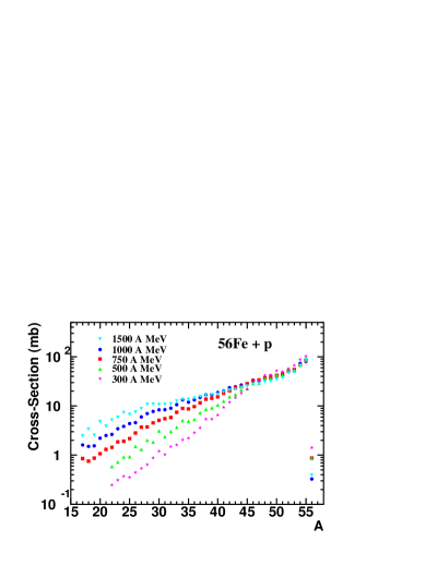
Figure 10: Mass distribution of the residual nuclei in the spallation reaction ${}^{56}Fe+p$ at the five different beam energies.

III.2 Comparison with other experimental data

III.2.1 Reverse kinematics

The present data can be compared with the ones obtained by W. R. Webber and collaborators using the reverse kinematics method. Measurements were performed on either a thick CH2 target (from $\sim 2g/cm^{2}$ to $\sim 6g/cm^{2}$) subtracting the carbon contribution Web90 ; Webform ; Web902 , or a liquid-hydrogen target ($1.52g/cm^{2}$) Web ; Web1086 at SATURNE. In both cases, the fragments were detected with a telescope of scintillators and Cerenkov counters.

The charge distributions of the spallation residues for several iron beam energies from 330 to 1615 A MeV  Web1086 ; Webform ; Web902 have been measured down to Z around 15. In Fig. 11, these results (histograms), at beam energies close to ours, namely 1512, 1086, 724, 520 and 330 A MeV are compared with the present cross-sections (symbols) summed over masses to obtain the charge distribution. The overall agreement is satisfying in terms of variation with energy and charge of the residue. A systematic dependence of the element cross sections with the parity of Z is consistently observed in both experiments. The deviation factor, i.e. the average ratio between the two experiments has been calculated and is shown in Table 1. The cross-section for Z=24 at 1512 A MeV, for which the Webber value is much larger than the neighboring cross sections and inconsistent with a general trend, is excluded. At the three highest energies, it is perfectly compatible with the precisions of both experiments (5% to 20% for Webber et al. and 9% to 15% here). At 300 A MeV (330 A MeV), the discrepancy is larger but still acceptable considering the different energies (10%) of the two measurements. The highest value (1.28) for the deviation factor is found at 500 A MeV (520 A MeV). Although this could be caused by a particular experimental problem at this energy, it is still compatible within the respective errors, especially if one bears in mind that at low energy both errors are larger: in our case because of the large transmission correction and in the case of Webber because of corrections for secondary reactions. The same reasons could explain the fact that, for a given energy, the disagreement is increasing with decreasing Z values, as it can be seen in Fig. 11. Another argument is that if we plot charge-changing cross sections as a function of the beam energy for various charges, our results at 500 A MeV are $\sim$10% below a smooth interpolation based on the other measured energies whereas the Webber values are $\sim$20% above the interpolation.

Energy/A (MeV)	300	500	750	1000	1500
Deviation factor	$1.23$	$1.28$	$1.01$	$0.89$	$0.88$

Table 1: Average ratio of the charge-changing cross-sections measured by Webber et al. Web1086 ; Webform ; Web902 divided by the values from this experiment.

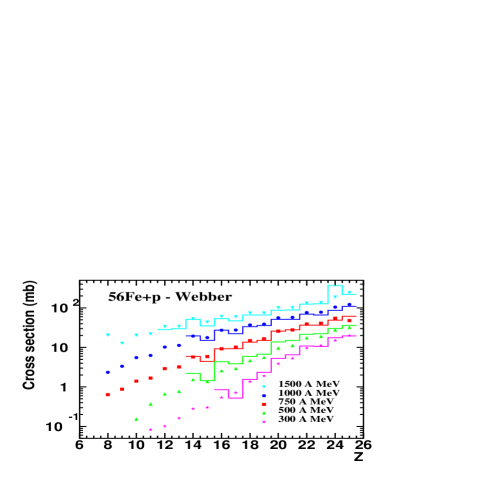
Figure 11: Nuclear-charge distribution of the residual nuclei for the five energies with scaling factors (2/1/0.5/0.25/0.125 respectively from 1500 A MeV to 300 A MeV) applied for clarity. Points correspond to the present data, and solid histograms are data from Webber et al.  Web902 ; Webform ; Web902 at close energies : 1512, 1086, 724, 520 and 330 A MeV.

The isotopic production cross-sections have also been measured previously but only at one energy (573 A MeV), using a liquid-hydrogen target Web ; Web1086 and were limited to rather large cross-sections. The ratio between these values and the present data is displayed in Fig. 12, including the respective errors. The lines represent the ratios of the cross sections at 573 A MeV and 500 A MeV computed with the INCL4-GEMINI combination of models. It shows that the difference in energy between the two experiments is not negligible for the lightest fragments, for which it can lead to differences of 30 to 40%. The agreement between the data is quite good for residues close in mass to iron but the difference increases for lighter isotopes. The value of the ratio is frequently hardly compatible with the expected value given by the line.

Figure 12: Ratio between isotopic cross-sections measured by Webber et al. at 573 A MeV Web ; Web1086 and the present experiment at 500 A MeV for each element as a function of the mass number. Lines are theoretical predictions from INCL4-GEMINI for this ratio.

Actually, one would expect a smooth variation of the mean value and of the width of the isotopic distribution with element charge. In Fig. 13 are represented the mean mass-over-charge ratio as the function of Z, summing only the isotopes measured by both experiments. Clearly these quantities are more fluctuating in the Webber et al. experiment, in particular for potassium (Z=19) data and to a smaller extent for argon (Z=18) and titanium (Z=22) ones. The use of our full isotopic distributions, which extend much beyond the ones of Webber et al., does not make a large difference.

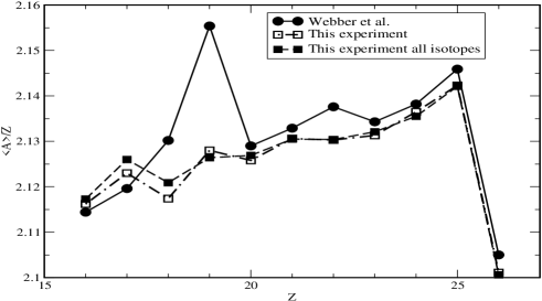
Figure 13: Ratio of the mean nuclear-mass value to the charge for each element measured by Webber et al. at 573 A MeV Web ; Web1086 (black circles) and in the present experiment at 500 A MeV (open squares). Black squares are for the same quantity evaluated from all isotopes measured in this experiment.

III.2.2 Direct kinematics

Results in direct kinematics have been obtained by R. Michel and collaborators Mic ; Mich97 ; Mich04 by irradiation of natural iron targets at different proton beam energies, allowing the determination of excitation functions from a few tens of MeV to about 2 GeV. Some of the produced residual nuclei have been measured and identified by their gamma-ray decay spectrum or by mass-spectrometry. These data are compared to our experimental data in Fig. 14 and Fig. 15. Results can be split into “cumulative” and “independent” nuclei meaning that they are or not populated by a decay chain. In the case of cumulative cross-sections, our own cross-sections have been summed along the decay chain before comparing with Michel’s data. The following isotopes: ${}^{36}Cl$ ${}^{42}K$, ${}^{46}Sc$, ${}^{48}Sc$ ${}^{54}Mn$ and ${}^{52}Fe$ are “independent”.

Our data follow quite well, in most of the cases, the dependence on energy obtained in the Michel et al. experiment. This is very satisfying if we consider the difference between the two experimental methods. Some of the important differences that can be noticed may be due to the use of natural iron in the case of Michel’s data. For instance, the observed higher cross-section for ${}^{52}Fe$ could come from a contribution of the (p,2n) reaction on ${}^{54}Fe$ adding to the (p,4n) on ${}^{56}Fe$. Although there is only 6% of ${}^{54}Fe$ in natural iron, the effect should be non-negligible since (p,2n) is 40 times more probable than (p,4n) as deduced from our results. Conversely, the lower cross-sections found by Michel for ${}^{52}Mn$ and the higher one for ${}^{56}Co$ at high energy do not seem compatible with the tendency deduced from our isotopic distributions.

Figure 14: Excitation functions of some residual nuclei produced in the spallation reaction of proton on iron. Open dots are the data of R. Michel et al. obtained by a direct irradiation Mich97 ; Mich04 and black triangles correspond to the present experimental data at 5 energies. Independent isotopes are indicated (Ind.).

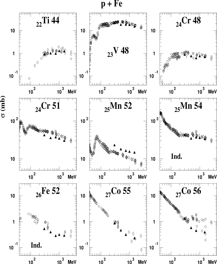
Figure 15: Excitation functions of some residual nuclei produced in the spallation reaction of proton on iron. Open dots are the data of R. Michel et al. obtained by a direct irradiation Mich97 ; Mich04 and black triangles correspond to the present experimental data at 5 energies. Independent isotopes are indicated (Ind.).

Finally, we can say that the present results are qualitatively in good agreement with former measurements. The fact that we have complete isotopic distributions extending down to lighter nuclei than previously measured, on a wide range of energy, allows us to check the consistency of our own results and detect possible inconsistencies in other sets of data.

III.3 Comparison with parametric formulas

Since 1950, parametric formulas have been developed by astrophysicists with the aim of predicting the production cross-sections of the residual nuclei in spallation reactions. These formulas are used in case of light and intermediate nuclei present in the composition of the cosmic-rays like iron. In this section we present the comparison of our new experimental data with the results of three of these parametric formulas: Webber Webber , EPAX Summerer and Silberberg and Tsao ST90 ; ST98 formulas.

III.3.1 Webber’s formula

This parametric formula has been developed by Webber et al. Webber from the experimental data shown in the previous section. It is used in case of light spallation residues with $Z_{i}<28$ and for energies of the projectile $E>200$ MeV.

The form of this formula is :

$$\sigma(A_{i},Z_{i},E)=\sigma_{0}(Z_{i},Z_{t})\cdot f_{1}(Z_{i},A_{i},Z_{t},A_{t})\cdot f_{2}(E,Z_{i},Z_{t})$$

for residual nuclei $(Z_{i},A_{i})$ of the spallation reaction on a target nuclei $(Z_{t},A_{t})$ at energy $E$.

• The first factor $\sigma_{0}(Z_{i},Z_{t})$ gives the charge distribution of the residues

• $f_{1}(Z_{i},A_{i},Z_{t},A_{t})$ describes the isotopic curves (from their data at 573 MeV per nucleon)

• $f_{2}(E,Z_{i},Z_{t})$ gives the energy dependence

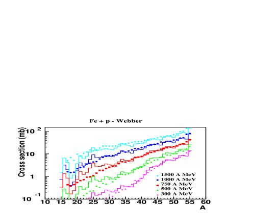
Figure 16: Comparison between present results at 5 energies (symbols) and the results obtained with Webber’s formula (solid lines). Scaling factors (2/1/0.5/0.25/0.125 respectively from 1500 A MeV to 300 A MeV) are applied for clarity.

In Fig. 16 the comparison of our mass distribution with the predictions of the Webber’s formula is shown. A rather good agreement is obtained at all the energies considered here for the heaviest residues, which are precisely those already measured by Webber et al. and used to determine the parameters of the formula. However, there seems to be some oscillations in the cross-sections not observed in the data. Actually, the charge distribution, not shown, is more accurately predicted by the formula. This comes from the fact that the isotopic distributions predicted by the Webber’s formula have smaller widths than those obtained experimentally (see Fig. 19). A probable explanation is that only very few isotopic data were existing at the time when the formula was established. Therefore, the isotopic dependence could not be properly determined. Furthermore, the extrapolation of the parametric formula for light residues that are measured here for the first time shows an important discrepancy with the data. Even if this parametric formula can be useful for determining the production of the most produced spallation residues, this illustrates the danger of using parametric formulas outside the range in which they were adjusted.

III.3.2 The EPAX formula

Epax formula Summerer was created with the aim of describing the production of residues in fragmentation reactions between heavy ions in what is call the limiting-fragmentation regime in which the residue production cross-section does not depend anymore on the energy of the projectile. Although not fully valid for protons at these energies, it might be instructive to know how close its predictions are to the present data. The limiting-fragmentation regime for the spallation reaction Fe + p is expected to be reached for energies of a few GeV per nucleon so here we can just expect the 1.5 A GeV data to be comparable with it.

It can be used for spallation reactions with protons in the case of target nuclei of masses $18<A_{t}<187$, although developed mainly for heavy-ion reaction . It is composed by two factors :

$$\sigma(Z_{i},A_{i})=Y_{A}\cdot\sigma(Z_{prob}-Z_{i})$$

with :

• $Y_{A}$ a factor to describe the mass distribution of the fragments $(Z_{i},A_{i})$
  

  $$Y_{A}=S_{2}(A_{t}^{1/3}+A_{pro}^{1/3}+S_{1})\cdot P\cdot exp[-P(A_{t}-A_{i})]$$

  and $lnP=P_{2}\cdot A_{t}+P1$. $S_{1}$, $S_{2}$, $P_{1}$ and $P_{2}$ being adjusted parameters and $A_{pro}$ the mass of the projectile (one here for protons).

• $\sigma(Z_{prob}-Z_{i})$ describes the isobaric curves with $Z_{prob}$ as the charge for the maximal production. The various $Z_{prob}$ values as a function of A defines the so called residue corridor in this approach.

In Fig. 17 our experimental results (symbols) are compared with the predictions of the EPAX formula. The experimental data at 1.5 GeV per nucleon are expected to be the ones closest to the limiting fragmentation regime, therefore we have renormalized the factor $S_{2}$ so that the formula gives the total reaction cross-section measured at 1.5 GeV per nucleon (794 mb). Since the EPAX total cross section was 617 mb, this led to a multiplication by 1.28.

It can be seen, as expected, that as the energy increases the mass distribution gets closer and closer to the EPAX prediction, with a quite good agreement at 1.5 GeV per nucleon. However, the lightest residues are still overestimated by the formula. The EPAX formula predicts also a more important evaporation of neutrons than seen in the isotopic cross-section data. In fact the measured N/Z ratio of the residues is higher than the one of the residue corridor which is used in the formula.

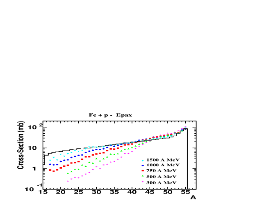
Figure 17: Comparison between the present measured mass distributions (symbols) and the results obtained with the EPAX formula (solid line).

III.3.3 Silberberg and Tsao’s formula

The first version of this parametric formula has been developed in 1973 ST73 with the experimental data measured by Rudstam Rud concerning the spallation residues in the spallation reaction $p+Fe$ at 340 MeV. Various improvements, especially the beam-energy dependence, have been added in successive versions ST90 ; ST98 . It can be written as :

$$\sigma(A,Z,E)=\sigma_{0}\cdot f(A)\cdot f(E)\cdot e^{-P(E)\Delta A}\cdot e^{-R|Z-SA-TA^{2}|^{\nu}}\Omega\cdot\eta\cdot\Phi$$

where :

• $\sigma_{0}$ is a normalization to the total reaction cross-section

• $f(A)$ and $f(E)$ are factors used only in the case of target nuclei $Z_{t}>30$

• $e^{-P(E)\Delta A}$ represents the reduction in the production cross-section with the mass difference ($\Delta A$) between the residue and the target nuclei and an energy dependence through the $P$ parameter

• $e^{-R|Z-SA-TA^{2}|^{\nu}}$ describes the width and the position of the maximum in the isotopic and isobaric production

• $\Omega$ takes into account the level structure of the residual nuclei

• $\eta$ is a factor for the pairing of protons and neutrons

• $\Phi$ represents an increase in the production of very light residues

In Fig. 18 a comparison of this formula with the experimental results presented in this work is shown. In general, the agreement is very good for all energies between 10 % and 30 % at 300 MeV per nucleon where the discrepancy is larger.

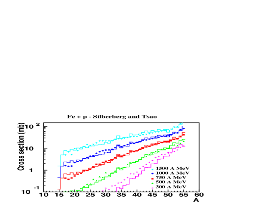
Figure 18: Comparison between present experimental results at the five energies (symbols) and the results obtained with the Silberberg and Tsao’s formula (solid lines). Scaling factors (2/1/0.5/0.25/0.125 respectively from 1500 A MeV to 300 A MeV) are applied for clarity.

This last parametric formula appears as the most suitable to reproduce the present data, probably because of the largest data base used to derive it, which contains systems rather close to the ones studied here. These formulas are quite useful for quickly calculating production rates. Although some physical ingredients are present to derive them, more sophisticated approaches are needed to better handle the physics included in spallation reactions and to describe more fully other observables than cross-sections.

III.3.4 Isotopic distribution shapes

Figure 19: Mean values and width of the mass-over-charge distributions as a function of element charge measured at 1500 MeV per nucleon compared with the predictions of the parametric formulas of Webber (solid line), Silberberg-Tsao (dashed-dotted line) and EPAX (dashed line).

In the preceding sections only mass distributions were compared to the predictions of the parametric formula. It is also interesting to know how they reproduce the isotopic distributions. A powerful way to look at this is to compare the shape of the mass distributions of each element through the mean value and width of the mass-over-charge distributions as a function of Z. This is what is shown in Fig. 19 in which the experimental results at 1500 MeV per nucleon (for better chance of agreement of EPAX) are compared with the three parametric formula. It can be seen that, as concerns the mean mass-over-charge, Webber’s formula and EPAX agree rather well with the data while Silberberg-Tsao’s predicts a slightly too high value. Regarding the widths, EPAX is acceptable and Webber tends to produce a too narrow mass distribution, maybe because the formula was fitted on his isotopic data which have a rather limited extension. Silberberg-Tsao gives a nearly constant width with Z, in contradiction to the experimental shape. This means that this formula, which gave the best agreement for mass distribution, should be used with caution if one wants to estimate isotope production cross-sections.

III.4 Comparison with models

The design and optimization of spallation sources requires the knowledge of a large number of quantities directly related to spallation reactions in different materials and at various energies. Since exhaustive measurements of such a large amount of data are beyond the experimental possibilities, one needs to develop spallation models with a good predictability that can be used in transport codes for simulations. This implies a deeper knowledge of the physics of the spallation reactions.

Spallation is generally described by a two-step mechanism. The first stage of intra-nuclear cascade process (INC) governed by nucleon-nucleon collisions, leads to an excited nucleus after the ejection of a few energetic particles (p, n, $\pi$, d, $\alpha$ etc.). The second longest phase follows corresponding to the evaporative decay of the excited remnant nucleus with a possible competition with fission and Fermi break-up in some cases. Some approaches include also an intermediate stage of pre-equilibrium to account smoothly for the transition to the full thermalization of the evaporating nucleus.

Old INC models are still currently used in the high-energy transport codes employed for applications as Bertini Bertini or ISABEL Isabel ) models. However, recently, a renewed interest for INC codes has been triggered by new available spallation data. Among them one could cite recent improvements on the INC codes found in INCL4 ; mashnik . In the present work, we have compared the experimental results of the spallation residues on iron to the predictions of three INC codes: Bertini code, ISABEL and INCL4 INCL4 . Since a long time, the first two ones are available in transport codes like LAHET3 lahet and MCNPX mcnpx for simulations of macro-systems, Bertini (with pre-equilibrium) being used by default. INCL4 was only recently implemented in these code systems as well as CEM mashnik . The basic physical assumptions are rather similar but differ in their implementation, for instance the way to develop the NN series of interactions, the way to treat Pauli blocking or the criterium to stop the INC stage. Note that we have used the implementation of ISABEL in LAHET3 which is blocked above 1 GeV. But this does not means that this cascade is not valid at higher energies.

For the second stage of the reaction, the most commonly used de-excitation code (and default option) in LAHET and MCNPX is the Dresner evaporation code Dresner complemented with the Atchison model for fission Atch . It uses the Weisskopf-Ewing formalism Weisskopf for the treatment of the evaporation, as do the more recent models ABLA ABLA and GEM GEM . Mainly, these three codes differ in the formulas and parameters used to described the level densities, the Coulomb barriers and the inverse reaction cross-sections. The Dresner code includes only the evaporation of light particles: neutrons, hydrogen and helium isotopes. The ABLA code has been mainly tuned for heavy systems with a particular interest on the fission description. In the version used in this work only neutrons, protons and alpha particles are evaporated. Furthermore shell and pairing effects as well as gamma decay were not taken here into account. The GEM code is a recent update of the Dresner model with new parameters and extends the Weisskopf-Ewing formalism to the evaporation of intermediate-mass fragments up to Z = 12. Actually the three codes (Dresner, ABLA and GEM) do not take into account in the evaporation process the angular momenta, which in fact are relatively small in spallation reactions induced by incident protons. Fission of heavy systems is described in a Bohr and Wheeler approach using phenomenological fragment distributions in Atchison and GEM. In ABLA fission is treated as a dynamical process taking into account the nuclear viscosity, and the fragment distribution is essentially obtained through the calculated population of states above the mass-asymmetric conditional saddle point.

As will be shown in the following, conventional Weisskopf-Ewing evaporation may be not sufficient to account for our data. This is why we will also compare our results to models predicting the emission of intermediate-mass fragments through other mechanisms. The GEMINI model gemini treats evaporation of light particles within the Hauser-Feshbach formalism hf , taking explicitly into account the angular momentum. Following the idea of Moretto moretto that there should be a continuous transition between evaporation and fission, for all systems including light ones, the emission of intermediate fragments is handled as asymmetric fission in the Transition State Model. The transition between Hauser-Feshbach evaporation and asymetric fission can be chosen through a parameter: in the present work, this parameter has been set so that the Transition State Model is used for fragments above helium. Several other options exist in the code. We have used the ones recommended by the author. Some tries to vary them, although not exhaustive, do not reveal strong differences in the description of the present data.

The SMM code is a numerical implementation of the Statistical Multifragmentation Model from smm often used to describe heavy-ion collisions in which multifragmentation is more likely to arise. The parameters to describe the multifragmentation process are the standard ones as described in eos . In particular, the asymptotic freeze-out volume is three times the initial one. The evaporation is treated in the Weisskopf-Ewing formalism up to fragment mass 18, and the lightest primary fragments decays are treated by the Fermi break-up fermi .

In the comparison between experimental data and model predictions, it is always difficult to disentangle the respective roles of the intra-nuclear cascade, which determines the characteristics of the remnant nucleus (charge, mass, angular momentum and excitation energy) at the end of the cascade stage, and of the de-excitation model. For instance, the under-prediction by the INCL4-ABLA combination of models of the light evaporation residue cross-sections observed for heavy systems Wla ; INCL4 could be ascribed either to a too low excitation energy given by INCL4 or to a deficiency of ABLA at the highest excitation energies. However, some observables can be found that are more sensitive to one reaction stage or the other. In the following, we will try, as far as possible, to disentangle the influences of the intra-nuclear cascade and of the de-excitation stage in the comparison with the different observables.

III.4.1 Total reaction cross-section

The total reaction cross-section is clearly one of the observables that depends only on the INC model since it is mainly related to the probability that the incident nucleon makes a collision with one nucleon of the target and that this collision is not blocked by the Pauli principle. In Fig. 20 we present the total reaction cross-sections obtained for the five energies analyzed in this work. They were calculated by summing up the isotope productions tabulated in the appendix. The summation has been done down to Z=8-10 depending on the bombarding energies. The contribution of the unmeasured isotopes have been estimated to be at most a few percents, i.e. smaller than the error bars. The fact that the lightest fragments could come from binary breakups and therefore leads to a possible double counting in the total reaction cross-section is also negligible. Actually, the two contributions play in opposit directions and even more or less compensate. Previous experimental data from the Barashenkhov compilation secreac are also shown on this figure. A reasonable agreement is observed between most of the previous data and the present ones for both the absolute values and the behavior with the incident energy. The predictions of all the three INC codes agree with the data within the experimental accuracy, the difference between them being at most 10 %. This is not surprising since these INC models are known to generally well reproduce the total reaction cross-sections at energy above a hundred MeV INCL4 ; lahet . This observable cannot be used to discriminate between these three codes.

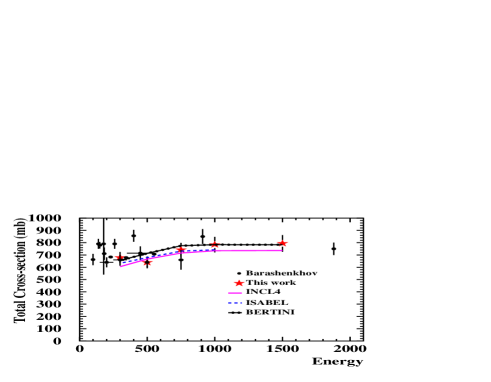
Figure 20: Total reaction cross-sections of protons on iron as a function of the bombarding energy. Our five experimental data are compared to the compilation of previous experimental data from Barashenkhov secreac and the values given by the three INC codes : Bertini, ISABEL (not available for E $>$ 1 GeV in LAHET3) and INCL4.

III.4.2 Mass and charge distributions

In this section we examine the various model predictions compared to the mass or charge distributions obtained by summing the measured isotopic cross-sections. For completeness the light fragment cross sections analyzed in Paolo and obtained during the same experiment are also included at 1 GeV per nucleon.

Figure 21: Mass distribution of the spallation residues of iron at 1 A GeV compared to the Bertini and INCL4 INC models combined with the Dresner evaporation code.

We first investigate the influence of the choice of the INC model. In Fig. 21 the mass and charge distributions of the residual nuclei produced at 1 GeV is shown and compared to the Bertini intra-nuclear cascade (plus pre-equilibrium) followed by the Dresner evaporation. Both mass and charge distributions lead to the same conclusions. The production yields of residues close to iron which are the major part of the spallation cross-section are underestimated while the yield of intermediate-mass residues is on the contrary overpredicted. The same conclusions were already obtained for heavy nuclei Wla . This behavior could be ascribed to a too high excitation energies at the end of the Bertini intranuclear cascade even after the introduction of a preequilibrium phase. A comparison is also shown with INCL4 followed by the same evaporation code. The calculations now predicts less excited remnants and a more satisfactory agreement is obtained for the heaviest residues but the light ones are still underestimated. It can be also noticed that, in both cases, the production of very light fragments is by far underpredicted. Another comparison is shown in Fig. 22 between the mass distribution of the spallation residues and the predictions of two different INC models, now ISABEL and INCL4, followed by the ABLA evaporation. This last combination has been shown to reproduce satisfactorily many spallation data INCL4 in a wide domain and without adjustment of parameters. Both calculations give a similar good descriptions of the residues close to iron and an underprediction of intermediate and light nuclei cross-sections. This underprediction of INCL4-ABLA is in fact consistent with light evaporation residue cross-sections obtained from heavier nuclei (lead and gold)  INCL4 . Actually, for the heaviest nuclei which are mainly formed in peripheral collisions with low excitation energy, the evaporation plays a less important role than the intra-nuclear cascade since only a very little number of nucleons is evaporated. The fact that both calculations have the same behavior and are rather good for heavy residues suggests that the underprediction of the light residues is not due to a lack of excitation energy. Indeed, we have seen in the comparison with Bertini in Fig. 21 that a larger excitation energy does lead to a larger production of light fragments but to the detriment of heavy ones which cannot be counterbalanced by playing with evaporation models. This rather indicates that the problem comes from the de-excitation stage. In the following we will not consider anymore the Bertini model for which many shotcomings have been pointed out sylvie , Wla , ab . We will mainly restrict the comparisons with various de-excitation models using INCL4 in the first stage, since ISABEL generally gives similar results.

Figure 22: Mass distribution of the spallation residues of iron at 1 A GeV compared to two different INC codes (INCL4 INCL4 and ISABEL Isabel ) combined with the ABLA evaporation code  ABLA .

Figure 23 shows the INCL4 intranuclear cascade coupled with the GEM model, which takes into account also evaporation of intermediate-mass fragments. The calculated cross-sections for the intermediate mass residues are improved comparatively to ABLA. However one observes a slight underestimation of the residues close to iron and the underprediction of the very light fragments still persists for masses slightly smaller than with ABLA.

From the comparison with the three evaporation models (Dresner, ABLA and GEM) and the remark concerning excitation energy made above, it can be presumed that standard evaporation models, even including the emission of IMF (GEM), cannot reproduce the bulk of our data. This is why we tried other models which include other de-excitation modes.

On Fig. 23, are also shown the predictions of GEMINI. If on the heavy fragments the results are slightly less satisfactory than with GEM, the behaviour for A lower than 30 is significantly improved. Probably due to its capability of predicting asymmetric fission in the Transition State Model prescription, GEMINI appears as the best suited code to reproduce the bulk of the data except at the lower energy (300 MeV per nucleon). Actually at 300 MeV per nucleon, all the calculations, whatever the choice of INC or de-excitation models, start to deviate from experiment around A equal 48.

Even-odd disymmetry of the cross sections are clearly visible on an unlarged picture of the Z distribution at 1 GeV per nucleon in Fig. 24 representative also of other energies. In spite of a small underprediction of the absolute cross-sections with GEMINI, the ratios between odd and even Z cross-sections are very close to the experimental ones. Whereas GEM gives a too strong effect, ABLA predicts (with the present version) a slightly too small even-odd effect. But for the largest cross-sections above 18 the INCL4-ABLA remains the more precise prediction of the experimental values.

Figure 23: Spallation residue cross-sections of iron as a function of there mass number compared with a calculation with INCL4 coupled with GEM (dashed lines) or GEMINI (continuous lines). Points are data of the present paper complemented for low masses at 1 GeV by the ones of  Paolo obtained during the same experiment.

Figure 24: Charge distribution of the spallation residues of iron at 1 A GeV compared to the INCL4 cascade coupled to the deexcitation models GEM, GEMINI and ABLA.

Another mechanism that could be invoked to explain our large yields of light fragments could be the onset of multifragmentation at the highest excitation energies Paolo . The coupling of INCL4 with the multifragmentation model, SMM, is shown in Fig. 25. The model well describes the heavy residues and the ones with mass between 20 and 30. However, it overpredicts the lighest fragments and disagrees strongly with the data in the A region 30-45. The contribution of fragments produced by multifragmentation is shown as the dashed curve in the figure (multifragmentation events being identified by the entry into the multifragmentation routine in the code Bot ). The major part of the light fragment cross-section is produced by multifragmentation while masses above 25 are mostly originating from evaporation. However, it is likely the opening of multifragmentation that causes the hole in the region $A=30-45$, not observed experimentally. Our results are at variance with what was found in Paolo , where SMM coupled to another INC model (from cem ) was giving a good agreement with the data, provided that a pre-equilibrium stage was added. With INCL4, which as explained in INCL4 , handles what is often called the pre-equilibrium stage, the best agreement with the whole set of data is obtained with GEMINI.

Figure 25: Calculation of the cross sections with INCL4 and SMM (solid line) compared to data points at 1 A GeV. The multifragmentation contribution to the calculation is the dashed line.

However, a clear conclusion on the mechanism responsible for the light and intermediate fragment production is difficult and would need more constraining information. It seems rather clear that the traditional Weisskopf-Ewing evaporation as used in ABLA or even in GEM, which evaporates IMFs, miss the production of the lighest nuclei. However, the reason for the success of GEMINI, Hauser-Fesbach treatment or asymmetric fission from the Transition-state-model, is not fully understood and a possible contribution of multifragmentation is not ruled out. Forthcoming exclusive experiments will probably help to clarify the situation by an identification of the various fragments emitted in coincidence during the de-excitation stage of the reaction.

III.4.3 Isotopic distributions

In this experiment, more than 500 individual isotopic cross sections have been measured which have been compared systematically to calculations done with the four different de-excitation codes (ABLA, GEM, GEMINI and SMM) coupled with INCL4. As an example, the comparison of GEMINI (full line) and ABLA (dashed line) with a selection of measured isotopic cross sections at 1 A GeV is shown on Fig. 26. Except for the better level of cross sections for light residues from GEMINI, already seen when looking at the mass distributions, it is difficult to conclude about the detailed quality of each model.

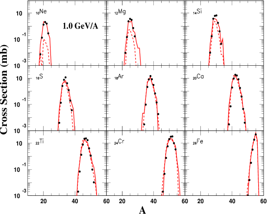
Figure 26: A selection of isotopic distributions of cross-sections measured at 1 A GeV compared with INCL4-GEMINI calculations (continuous lines) and INCL4-ABLA (dashed lines).

A more powerfull way to make the comparison is to look at the shapes of the isotopic distributions for each element through the mean atomic mass ($\langle A\rangle$) divided by the charge Z of the element and the width (root mean square) of the measured (or computed) distributions. Figure 27 presents the comparison of these quantities with GEMINI at the five energies while Fig. 28 shows the results INCL4 coupled to either ABLA, GEM or SMM at 1 A GeV. Actually, it is remarkable that the deviations between models and experiment are qualitatively independent of the beam energy. This can be checked on Fig. 27 for GEMINI but holds also for the comparison with the other models. For this reason, the comparison with the other three models is shown only at 1 A GeV in Fig. 28. But again, the following conclusions are the same at all the energies.

For Z equal 25, 26 and 27 (not measured at 1 A GeV), cross sections are dominated by the cascade, leaving the remnant nucleus with very little excitation energy. Therefore, the choice of the evaporation model play practically no role and basically the $\langle A\rangle/Z$ is perfectly reproduced. The average value of the isotopic distribution ($\langle A\rangle/Z$) is actually very well predicted by GEM and GEMINI on all the range (down to Z equal 8 to 9), with the correct odd-even effects, whereas ABLA gives a value systematically too small. The SMM model gives a correct centroid down to Z equal 20 but is the worst below this value with a distribution centered one mass below the data at lower Z. As regards the width of the distributions, none of the models is good on all the Z range. The widths computed from GEMINI are systematically a little too wide. With GEM and ABLA, they are too wide only in the range 20-25, otherwise they are very close to the data. For SMM, it is the contrary, rather good at high Z but too narrow for lower charges. This fact was already noticed in Souza .

All this shows that none of the de-excitation models is perfect. However, taking into account the information from both the cross-sections and the isotopic distribution shapes, it can be concluded that the GEMINI gives the best agreement with our data.

Figure 27: Mean atomic mass A over Z ($\langle A\rangle/Z$) and rms ($\sigma(A)$) of the isotopic cross section distributions as a function of the atomic number Z, at the five bombarding energies, compared to calculations done with the intranuclear cascade INCL4 model coupled with GEMINI. The calculated values have been averaged over the actually measured isotopes.

Figure 28: Same as fig 27 but only at 1 A GeV for comparison with calculations done with the intranuclear-cascade INCL4 model coupled with ABLA (full line), GEM (dashed line), and SMM (dashed-dotted line).

III.4.4 Recoil velocities.

Concerning the kinetic characteristics of the fragments, we show in Fig. 29 a comparison between the experimental mean longitudinal recoil velocities for each mass and the ones calculated with the INCL4 model combined with ABLA or GEMINI at 1 A GeV. The same comparison is also done for the width (root mean square) of the longitudinal distribution (right part of the figure).

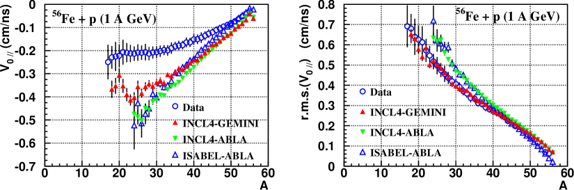
Figure 29: Mean (left) and Root Mean Square (right) values of the longitudinal recoil velocity distribution for spallation residues at 1 A GeV versus their atomic mass. Open circles are the experimental values. Down triangles are predictions from the INCL4-ABLA calculation, up empty triangles from the ISABEL-ABLA and up full triangles from the INCL4-GEMINI calculation. Velocities are expressed in the beam (${}^{56}Fe$) rest frame and with a minus sign as being opposite to the iron beam direction.

One can observe an important discrepancy between the experimental mean recoil velocities and values predicted by the models. It is worthwhile to note that the experimental data decrease much more slowly with decreasing mass than the values predicted by the codes. Furthermore, they seem to saturate at a mass value of 35. This saturation is not seen with ABLA. Only GEMINI shows a clear tendency towards saturation below A=30. For the widths, on the contrary, the agreement with the experimental data is better, especially when using GEMINI. This behavior, presented here at 1 GeV, is very similar at the others energies analyzed in this experiment (Fig. 30). The better agreement with GEMINI could be due to the existence of binary decays in de-excitation phase that reduces the mean longitudinal velocity of the final residual nuclei since the recoil momentum will originate from a heavier nucleus and will be split between two partners emitted in an arbitrary direction with respect to the beam one. In the same figure, are also shown the predictions from systematics of Morrisey Morri , which more or less give the correct slope for large mass but miss the saturation observed in the data. Actually, the two other de-excitation models GEM and SMM, not shown here, give results rather similar to ABLA: rather good for the widths but a slope too steep and an inability to describe the saturation of the mean values.

The fact that the mean recoil velocities for the heaviest masses is not well predicted cannot be ascribed to the de-excitation models but should rather raise questions on the intranuclear cascade. This is why we have also performed a calculation using ISABEL coupled to ABLA, which is presented in Fig. 29. Obviously, ISABEL better reproduces both the mean values and the widths for masses larger than 50, indicating a possible deficiency of INCL4 in the recoil velocity determination. Actually, a similar systematic deviation of INCL4 concerning the mean velocities has already been noticed for Pb+p at 1 GeV/A Wla . However, the general trend of the ISABEL calculation on the whole mass range leads to the same conclusion that it is unable to give the correct slope and saturation effect of the experimental data.

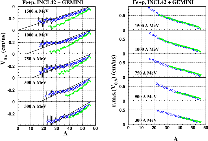
Figure 30: Mean values and r.m.s. of the longitudinal recoil velocity distribution for spallation residues versus their atomic mass at all beam energies. Open circles are experimental values. Down triangles are predictions from the INCL4 + GEMINI calculation. The lines are the Morrissey systematics Morri .

IV Conclusion

The spallation residues produced in the bombardment of ${}^{56}Fe$ at 1.5 , 1.0, 0.75, 0.5 and 0.3 A GeV on a liquid-hydrogen target have been studied using the reverse kinematics technique and the Fragment Separator at GSI (Darmstadt). This technique has permitted the full identification in charge and mass of all isotopes produced with cross-sections larger than $10^{-2}$ mb down to $Z=8$. Their individual production cross-sections and recoil velocities at the five energies have been obtained.

The production cross-sections have been compared with the previously existing data, either charge-changing cross-sections with a few isotopic cross-sections at one energy measured in reverse kinematics or excitation functions for a limited number of isotopes obtained by $\gamma$-spectrometry in direct kinematics. Globally, our results were found in good agreement with former data. This comparison also showed that our experimental method leads to a much more complete picture of the residue production than what was possible before with the few scattered results, allowing sometimes to detect possible inconsistencies in other sets of data.

Comparisons with parametric formulas, often used in astrophysics, have been performed: the Webber formula gives rather good predictions of the charge distributions but produces too narrow isotopic distributions. It also totally fails for the lightest nuclei (below A equal 30-35) in the region not measured at the time when this formula was derived. The EPAX formula (once renormalized to give the correct total reaction cross-section) is usable only in the limiting fragmentation regime, apparently not yet fully reached at 1.5 A GeV. However, it nearly gives the right A dependence of the cross sections at our highest energy. The best formula seems to be the Silberberg and Tsao one, which is in very good agreement with the experimental mass distributions and mean value of the isotopic distributions at all the energies except at 300 MeV (as all the models). The use of parametric formulas can be of great help for a fast estimation for certain applications, but the example of Webber’s illustrates the possible danger of using parametric formulas outside the range on which they have been adjusted. Our data could certainly be used to derive new, more relaible parametric formulas for use in cosmic-ray propagation codes.

Predictions of different intranuclear-cascade models (Bertini, ISABEL and INCL4) combined with different de-excitation models (Dresner, ABLA, GEM, SMM and GEMINI) have been confronted to the new experimental data. INCL4 or ISABEL combined with standard Weisskopf-Ewing evaporation models as ABLA or GEM give a good description of the residual production close in charge to iron but they underpredict systematically the light evaporation residues in the mass region 20-30. This fact, together with the saturation observed in the experimental longitudinal velocity at low masses, could be an indication that another de-excitation mechanism has to be considered. A de-excitation including a possible contribution from multifragmentation, as treated by SMM, improves significantly the predictions of light and intermediate mass fragments but at the detriment of residues in the region $A=30-45$. SMM also misses the saturation of the recoil velocity and do not properly predict the isotopic distribution mean values and widths. The best overall agreement with the data is obtained with GEMINI. This GEMINI model gives a rather precise account of all cross sections measured here as a function of the beam energy. The recoil velocities, although not perfect, are the closest to the experimental values and the mean values and widths of the isotopic distributions are rather well reproduced. Other authors NESSI ; NESSI2 have found that generally GEMINI reproduces very well the energy spectra of both light charged particles and intermediate mass fragments in a wide range of incident energies and target masses. Similar conclusions (best agreement with GEMINI) have been reached by maschnik_santafe using as intra-nuclear model the Cascade-Exciton Model, coupled with GEM, GEMINI and SMM and compared with these data taken from the C. Villagrasa-Canton PhD  cv_these . In Paolo , with another INC coupled with a preequilibrium stage, the deexcitation code SMM was found to give the best agreement with the 1 GeV data. It is obviously difficult to definitively conclude on the production mechanism of the intermediate and light mass fragments and probably only additional experimental information on correlations between residual nuclei and light particles could bring aswers to the questions addressed here.

As regards to the potential interest of the present data for applications, we supply isotopic cross-sections that can be used to directly estimate the change in chemical composition that could occur in an ADS window made predominantly of iron and recoil velocities to calculate damages due to atomic displacements (DPA) cv_these .

V Acknowledgements

This experiment has benefited from a flexible and efficient driving of the GSI accelerators. Many thanks to all the driving team. The technical support of K.H. Behr, A. Brünle and K. Burkard was crucial for the preparation of the experimental setup, and the liquid target was smoothly managed by P. Chesny, J.M. Gheller and G. Guiller. We thank them all for their contribution. Comparison with irradiation experiments (fig 14 and 15) was possible due to the help of J.C. David and due to the kindness of Pr. R. Michel providing us the experimental file. We thank also A. Botvina for helping us to identify the multifragmentation contribution in the SMM code.

During the interpretation of these results, we have benefited from fruitful discussions with J. Cugnon and Y. Yariv.

VI Appendix A: Cross sections.

		1500 A MeV			$\sigma_{R}(mb)=822\pm 73$
Z	A	$\sigma(mb)$	Z	A	$\sigma(mb)$	Z	A	$\sigma(mb)$
27	54	0.035$\pm$0.0021	23	50	16.272$\pm$2.383	20	44	8.0592$\pm$0.798
27	55	0.245$\pm$0.0104	23	51	7.179$\pm$0.446	20	45	1.8149$\pm$0.174
27	56	0.413$\pm$0.0187	23	52	1.274$\pm$0.073	20	46	0.4263$\pm$0.039
26	51	0.016$\pm$0.0021	23	53	0.251$\pm$0.012	20	47	0.0497$\pm$0.004
26	52	0.309$\pm$0.0187	23	54	0.004$\pm$0.001	20	48	0.0052$\pm$0.001
26	53	2.865$\pm$0.1338	22	43	0.093$\pm$0.009	19	37	0.0683$\pm$0.008
26	54	22.204$\pm$0.8962	22	44	1.309$\pm$0.129	19	38	1.2762$\pm$0.141
26	55	58.838$\pm$2.2010	22	45	7.067$\pm$0.675	19	39	8.4339$\pm$0.918
25	49	0.018$\pm$0.0021	22	46	19.052$\pm$1.767	19	40	12.7248$\pm$1.364
25	50	0.329$\pm$0.0249	22	47	20.863$\pm$1.941	19	41	10.0161$\pm$1.076
25	51	3.612$\pm$0.2240	22	48	15.246$\pm$1.957	19	42	4.2599$\pm$0.443
25	52	15.089$\pm$0.8523	22	49	4.051$\pm$0.325	19	43	1.4303$\pm$0.147
25	53	37.982$\pm$1.7678	22	50	1.078$\pm$0.081	19	44	0.2596$\pm$0.026
25	54	42.812(Interp.)	22	51	0.103$\pm$0.006	19	45	0.0434$\pm$0.004
25	55	32.885$\pm$1.2297	22	52	0.011$\pm$0.001	19	46	0.0041$\pm$0.001
24	46	0.002$\pm$0.0004	21	41	0.027$\pm$0.004	18	35	0.1706$\pm$0.020
24	47	0.054$\pm$0.0052	21	42	0.918$\pm$0.097	18	36	2.7062$\pm$0.304
24	48	0.724$\pm$0.0622	21	43	6.840$\pm$0.702	18	37	8.8348$\pm$0.985
24	49	5.043$\pm$0.4032	21	44	14.639$\pm$1.447	18	38	14.1045$\pm$1.551
24	50	18.522$\pm$1.3723	21	45	17.225$\pm$1.687	18	39	8.6291$\pm$0.947
24	51	27.886$\pm$1.7288	21	46	8.934$\pm$1.004	18	40	3.0793$\pm$0.331
24	52	31.954$\pm$4.2184	21	47	2.989$\pm$0.267	18	41	0.7825$\pm$0.084
24	53	10.052$\pm$0.4695	21	48	0.572$\pm$0.049	18	42	0.1602$\pm$0.017
24	54	3.848$\pm$0.1565	21	49	0.093$\pm$0.007	18	43	0.0207$\pm$0.002
24	55	0.054$\pm$0.0021	21	50	0.006$\pm$0.001	18	44	0.0021$\pm$0.001
23	45	0.046$\pm$0.0041	20	39	0.105$\pm$0.011	17	33	0.0837$\pm$0.009
23	46	0.693$\pm$0.0642	20	40	2.115$\pm$0.227	17	34	1.6685$\pm$0.192
23	47	5.372$\pm$0.4797	20	41	9.204$\pm$0.982	17	35	8.7775$\pm$1.001
23	48	15.447$\pm$1.3179	20	42	16.363$\pm$1.695	17	36	10.6805$\pm$1.203
23	49	23.728$\pm$1.9001	20	43	14.268$\pm$1.500	17	37	6.9602$\pm$0.815

		1500 A MeV
Z	A	$\sigma(mb)$	Z	A	$\sigma(mb)$	Z	A	$\sigma(mb)$
17	38	1.872$\pm$0.2066	14	29	8.920$\pm$1.055	11	25	1.0696$\pm$0.130
17	39	0.536$\pm$0.0589	14	30	8.572$\pm$1.042	11	26	0.1719$\pm$0.021
17	40	0.098$\pm$0.0103	14	31	2.549$\pm$0.314	11	27	0.0309$\pm$0.003
17	41	0.018$\pm$0.0021	14	32	0.626$\pm$0.073	10	19	0.2531$\pm$0.032
16	31	0.027$\pm$0.0031	14	33	0.072$\pm$0.008	10	20	3.2281$\pm$0.402
16	32	3.679$\pm$0.4306	14	34	0.015$\pm$0.002	10	21	3.1828$\pm$0.446
16	33	9.282$\pm$1.0728	13	25	0.246$\pm$0.030	10	22	3.0172$\pm$0.389
16	34	11.562$\pm$1.3826	13	26	2.751$\pm$0.331	10	23	0.5833$\pm$0.071
16	35	4.865$\pm$0.5648	13	27	7.469$\pm$0.886	10	24	0.1378$\pm$0.016
16	36	1.547$\pm$0.1745	13	28	4.550$\pm$0.545	9	17	0.2251$\pm$0.029
16	37	0.259$\pm$0.0289	13	29	2.090$\pm$0.325	9	18	1.8555$\pm$0.234
16	38	0.047$\pm$0.0052	13	30	0.366$\pm$0.043	9	19	2.0827$\pm$0.301
16	39	0.007$\pm$0.0010	13	31	0.078$\pm$0.009	9	20	1.7157$\pm$0.249
15	29	0.171$\pm$0.0206	12	23	0.498$\pm$0.061	9	21	0.5777$\pm$0.072
15	30	2.126$\pm$0.2508	12	24	4.837$\pm$0.589	9	22	0.0874$\pm$0.010
15	31	8.475$\pm$0.9959	12	25	5.600$\pm$0.676	8	16	6.2764$\pm$0.799
15	32	7.057$\pm$0.8514	12	26	4.813$\pm$0.583	8	17	2.3020$\pm$0.364
15	33	3.707$\pm$0.4303	12	27	1.185$\pm$0.142	8	18	1.6292$\pm$0.270
15	34	0.851$\pm$0.0980	12	28	0.315$\pm$0.038	8	19	0.2845$\pm$0.035
15	35	0.193$\pm$0.0217	12	29	0.033$\pm$0.004	0	0	0.0000$\pm$0.000
15	36	0.022$\pm$0.0021	11	21	0.226$\pm$0.028	0	0	0.0000$\pm$0.000
15	37	0.002$\pm$0.0010	11	22	2.244$\pm$0.276	0	0	0.0000$\pm$0.000
14	27	0.453$\pm$0.0547	11	23	4.967$\pm$0.608	0	0	0.0000$\pm$0.000
14	28	6.317$\pm$0.7539	11	24	2.594$\pm$0.319	0	0	0.0000$\pm$0.000

		1000 A MeV			$\sigma_{R}(mb)=811\pm 76$
Z	A	$\sigma(mb)$	Z	A	$\sigma(mb)$	Z	A	$\sigma(mb)$
26	51	0.016$\pm$0.0010	23	52	1.259$\pm$0.071	20	44	8.6501$\pm$0.896
26	52	0.333$\pm$0.0187	23	53	0.246$\pm$0.011	20	45	1.8676$\pm$0.178
26	53	3.319$\pm$0.1556	23	54	0.004$\pm$0.001	20	46	0.4159$\pm$0.038
26	54	18.977$\pm$0.7686	22	42	0.002$\pm$0.001	20	47	0.0476$\pm$0.004
26	55	47.982$\pm$1.7913	22	43	0.071$\pm$0.007	20	48	0.0041$\pm$0.001
25	49	0.017$\pm$0.0010	22	44	1.347$\pm$0.134	19	37	0.0455$\pm$0.005
25	50	0.373$\pm$0.0280	22	45	7.999$\pm$0.764	19	38	1.1211$\pm$0.123
25	51	3.971$\pm$0.2457	22	46	22.716$\pm$2.106	19	39	8.3398$\pm$0.909
25	52	15.927$\pm$0.9010	22	47	24.143$\pm$2.162	19	40	14.1478$\pm$1.517
25	53	39.583$\pm$1.8373	22	48	17.468$\pm$2.361	19	41	10.5654$\pm$1.169
25	54	46.679(Interp.)	22	49	4.245$\pm$0.340	19	42	4.4129$\pm$0.496
25	55	35.410$\pm$1.3189	22	50	1.162$\pm$0.086	19	43	1.3951$\pm$0.143
25	56	0.338$\pm$0.0135	22	51	0.100$\pm$0.006	19	44	0.2565$\pm$0.026
24	46	0.002$\pm$0.0010	22	52	0.010$\pm$0.001	19	45	0.0403$\pm$0.004
24	47	0.048$\pm$0.0041	21	41	0.019$\pm$0.002	18	34	0.0031$\pm$0.001
24	48	0.789$\pm$0.0674	21	42	0.882$\pm$0.091	18	35	0.1013$\pm$0.011
24	49	5.925$\pm$0.4737	21	43	7.427$\pm$0.762	18	36	2.2245$\pm$0.250
24	50	21.256$\pm$1.5765	21	44	17.367$\pm$1.717	18	37	8.4183$\pm$0.939
24	51	32.184$\pm$1.9900	21	45	19.221$\pm$1.837	18	38	14.8374$\pm$1.633
24	52	34.246$\pm$8.0637	21	46	10.876$\pm$1.470	18	39	8.6601$\pm$0.992
24	53	10.341$\pm$0.4799	21	47	3.198$\pm$0.286	18	40	3.1145$\pm$0.334
24	54	3.558$\pm$0.1430	21	48	0.586$\pm$0.050	18	41	0.7143$\pm$0.076
23	44	0.002$\pm$0.0010	21	49	0.089$\pm$0.007	18	42	0.1478$\pm$0.016
23	45	0.037$\pm$0.0031	21	50	0.005$\pm$0.001	18	43	0.0186$\pm$0.002
23	46	0.736$\pm$0.0684	20	38	0.003$\pm$0.001	17	32	0.0031$\pm$0.001
23	47	6.104$\pm$0.5450	20	39	0.074$\pm$0.008	17	33	0.0486$\pm$0.005
23	48	18.284$\pm$1.5613	20	40	2.012$\pm$0.215	17	34	1.2491$\pm$0.145
23	49	27.086$\pm$2.1654	20	41	9.679$\pm$1.033	17	35	7.8911$\pm$0.901
23	50	19.590$\pm$3.6884	20	42	18.973$\pm$1.966	17	36	10.3138$\pm$1.195
23	51	7.109$\pm$0.4393	20	43	16.390$\pm$2.018	17	37	6.7298$\pm$0.807

		1000 A MeV
Z	A	$\sigma(mb)$	Z	A	$\sigma(mb)$
17	38	1.608$\pm$0.1767	13	27	5.202$\pm$0.625
17	39	0.464$\pm$0.0506	13	28	3.173$\pm$0.384
17	40	0.080$\pm$0.0083	13	29	1.393$\pm$0.171
16	30	0.004$\pm$0.0010	13	30	0.229$\pm$0.027
16	31	0.138$\pm$0.0165	13	31	0.047$\pm$0.005
16	32	2.611$\pm$0.3056	12	22	0.010$\pm$0.001
16	33	7.803$\pm$0.9025	12	23	0.158$\pm$0.020
16	34	11.850$\pm$1.6129	12	24	2.482$\pm$0.309
16	35	4.211$\pm$0.4977	12	25	3.793$\pm$0.458
16	36	1.270$\pm$0.1425	12	26	3.160$\pm$0.381
16	37	0.202$\pm$0.0227	12	27	0.760$\pm$0.092
16	38	0.037$\pm$0.0041	12	28	0.178$\pm$0.022
15	28	0.004$\pm$0.0010	11	20	0.009$\pm$0.001
15	29	0.078$\pm$0.0093	11	21	0.087$\pm$0.011
15	30	1.355$\pm$0.1600	11	22	1.050$\pm$0.132
15	31	6.668$\pm$0.7843	11	23	3.091$\pm$0.389
15	32	6.284$\pm$0.9288	11	24	1.480$\pm$0.222
15	33	3.066$\pm$0.3622	11	25	0.629$\pm$0.076
15	34	0.623$\pm$0.0722	11	26	0.096$\pm$0.011
15	35	0.137$\pm$0.0155	10	18	0.007$\pm$0.001
14	26	0.010$\pm$0.0010	10	19	0.140$\pm$0.019
14	27	0.180$\pm$0.0217	10	20	1.381$\pm$0.178
14	28	3.852$\pm$0.4600	10	21	2.199$\pm$0.280
14	29	6.525$\pm$0.7746	10	22	1.664$\pm$0.210
14	30	7.040$\pm$0.8333	10	23	0.299$\pm$0.038
14	31	1.870$\pm$0.2269	9	17	0.072$\pm$0.009
14	32	0.431$\pm$0.0505	9	18	0.706$\pm$0.094
14	33	0.047$\pm$0.0052	9	19	1.452$\pm$0.196
13	24	0.006$\pm$0.0010	9	20	0.891$\pm$0.121
13	25	0.094$\pm$0.0113	9	21	0.300$\pm$0.037
13	26	1.449$\pm$0.1742	8	17	1.585$\pm$0.211

		750 A MeV			$\sigma_{R}(mb)=767\pm 66$
Z	A	$\sigma(mb)$	Z	A	$\sigma(mb)$	Z	A	$\sigma(mb)$
27	54	0.035$\pm$0.0021	23	50	19.689$\pm$2.487	20	44	8.3324$\pm$0.831
27	55	0.333$\pm$0.0145	23	51	7.647$\pm$0.473	20	45	1.8625$\pm$0.178
27	56	0.474$\pm$0.0228	23	52	1.270$\pm$0.073	20	46	0.3901$\pm$0.036
26	51	0.011$\pm$0.0010	23	53	0.225$\pm$0.010	20	47	0.0445$\pm$0.004
26	52	0.300$\pm$0.0176	23	54	0.003$\pm$0.001	20	48	0.0041$\pm$0.001
26	53	3.437$\pm$0.1628	22	43	0.045$\pm$0.004	19	37	0.0207$\pm$0.002
26	54	20.841$\pm$0.8433	22	44	1.016$\pm$0.100	19	38	0.7136$\pm$0.079
26	55	52.837$\pm$1.9738	22	45	7.983$\pm$0.763	19	39	7.2694$\pm$0.792
25	49	0.012$\pm$0.0010	22	46	22.428$\pm$2.081	19	40	11.9543$\pm$1.283
25	50	0.298$\pm$0.0228	22	47	25.267$\pm$2.274	19	41	9.2923$\pm$1.138
25	51	4.366$\pm$0.2717	22	48	18.309$\pm$1.823	19	42	3.6528$\pm$0.384
25	52	16.830$\pm$0.9529	22	49	4.577$\pm$0.367	19	43	1.3052$\pm$0.134
25	53	42.696$\pm$1.9835	22	50	1.145$\pm$0.085	19	44	0.2306$\pm$0.023
25	54	47.052(Interp.)	22	51	0.093$\pm$0.006	19	45	0.0372$\pm$0.003
25	55	34.496$\pm$1.2888	22	52	0.009$\pm$0.001	19	46	0.0031$\pm$0.001
25	56	0.429$\pm$0.0197	21	41	0.011$\pm$0.001	18	35	0.0413$\pm$0.005
24	47	0.034$\pm$0.0031	21	42	0.619$\pm$0.064	18	36	1.3831$\pm$0.156
24	48	0.653$\pm$0.0560	21	43	7.052$\pm$0.724	18	37	6.7799$\pm$0.757
24	49	6.143$\pm$0.4923	21	44	16.154$\pm$1.598	18	38	12.3038$\pm$1.355
24	50	22.252$\pm$1.6501	21	45	19.447$\pm$1.895	18	39	7.2843$\pm$0.817
24	51	34.636$\pm$2.1424	21	46	9.974$\pm$1.004	18	40	2.4932$\pm$0.269
24	52	35.666$\pm$6.1359	21	47	3.387$\pm$0.302	18	41	0.5592$\pm$0.060
24	53	10.957$\pm$0.5099	21	48	0.575$\pm$0.049	18	42	0.1034$\pm$0.010
24	54	3.408$\pm$0.1379	21	49	0.087$\pm$0.007	18	43	0.0155$\pm$0.002
24	55	0.037$\pm$0.0021	21	50	0.005$\pm$0.001	17	33	0.0196$\pm$0.002
23	45	0.023$\pm$0.0021	20	39	0.039$\pm$0.004	17	34	0.7211$\pm$0.084
23	46	0.569$\pm$0.0528	20	40	1.394$\pm$0.149	17	35	5.9777$\pm$0.686
23	47	6.337$\pm$0.5657	20	41	8.992$\pm$0.961	17	36	7.7320$\pm$0.873
23	48	18.897$\pm$1.6131	20	42	16.725$\pm$1.741	17	37	5.0809$\pm$0.578
23	49	30.515$\pm$2.4399	20	43	15.585$\pm$1.707	17	38	1.2656$\pm$0.141

		750 A MeV
Z	A	$\sigma(mb)$	Z	A	$\sigma(mb)$
17	39	0.322$\pm$0.0351	13	28	1.841$\pm$0.225
17	40	0.052$\pm$0.0052	13	29	0.714$\pm$0.087
16	31	0.046$\pm$0.0062	13	30	0.088$\pm$0.010
16	32	1.437$\pm$0.1683	13	31	0.020$\pm$0.002
16	33	5.539$\pm$0.6412	12	23	0.052$\pm$0.008
16	34	8.110$\pm$0.9386	12	24	1.193$\pm$0.147
16	35	2.919$\pm$0.3366	12	25	1.968$\pm$0.245
16	36	0.896$\pm$0.1012	12	26	2.149$\pm$0.277
16	37	0.113$\pm$0.0124	12	27	0.538$\pm$0.071
16	38	0.022$\pm$0.0021	12	28	0.071$\pm$0.008
16	39	0.003$\pm$0.0010	12	29	0.002$\pm$0.001
15	29	0.025$\pm$0.0031	11	21	0.030$\pm$0.005
15	30	0.664$\pm$0.0795	11	22	0.526$\pm$0.085
15	31	4.572$\pm$0.5449	11	23	1.810$\pm$0.251
15	32	4.348$\pm$0.6440	11	24	0.779$\pm$0.100
15	33	2.074$\pm$0.2477	11	25	0.249$\pm$0.031
15	34	0.368$\pm$0.0433	11	26	0.058$\pm$0.007
15	35	0.074$\pm$0.0083	10	20	0.638$\pm$0.103
15	36	0.005$\pm$0.0010	10	21	1.216$\pm$0.183
14	27	0.053$\pm$0.0072	10	22	0.968$\pm$0.166
14	28	1.964$\pm$0.2341	10	23	0.047$\pm$0.007
14	29	3.960$\pm$0.4765	10	24	0.014$\pm$0.002
14	30	4.510$\pm$0.5415	9	18	0.342$\pm$0.057
14	31	1.062$\pm$0.1289	9	19	0.897$\pm$0.162
14	32	0.239$\pm$0.0278	9	20	0.469$\pm$0.088
14	33	0.013$\pm$0.0021	9	21	0.097$\pm$0.014
14	34	0.004$\pm$0.0010	8	17	0.880$\pm$0.149
13	25	0.030$\pm$0.0041	8	18	0.431$\pm$0.083
13	26	0.702$\pm$0.0866	0	0	0.000$\pm$0.000
13	27	3.243$\pm$0.4247	0	0	0.000$\pm$0.000

		500 A MeV			$\sigma_{R}(mb)=660\pm 53$
Z	A	$\sigma(mb)$	Z	A	$\sigma(mb)$	Z	A	$\sigma(mb)$
27	53	0.003$\pm$0.0010	23	49	27.507$\pm$2.593	20	43	11.4146$\pm$1.372
27	54	0.059$\pm$0.0021	23	50	19.027$\pm$2.696	20	44	6.7186$\pm$0.745
27	55	0.485$\pm$0.0197	23	51	6.266$\pm$0.387	20	45	1.2635$\pm$0.121
27	56	0.611$\pm$0.0248	23	52	0.949$\pm$0.054	20	46	0.2558$\pm$0.024
26	51	0.020$\pm$0.0010	23	53	0.152$\pm$0.007	20	47	0.0268$\pm$0.002
26	52	0.416$\pm$0.0238	23	54	0.002$\pm$0.001	20	48	0.0021$\pm$0.001
26	53	3.855$\pm$0.1789	22	43	0.052$\pm$0.005	19	37	0.0227$\pm$0.003
26	54	23.507$\pm$0.9454	22	44	1.052$\pm$0.104	19	38	0.5010$\pm$0.056
26	55	56.647$\pm$2.1110	22	45	6.650$\pm$0.635	19	39	4.4844$\pm$0.489
25	49	0.019$\pm$0.0021	22	46	20.458$\pm$1.897	19	40	8.0008$\pm$0.859
25	50	0.387$\pm$0.0289	22	47	21.553$\pm$2.204	19	41	6.3328$\pm$0.763
25	51	4.490$\pm$0.2771	22	48	17.702$\pm$2.230	19	42	2.7133$\pm$0.313
25	52	18.309$\pm$1.0328	22	49	3.529$\pm$0.282	19	43	0.7948$\pm$0.081
25	53	42.027$\pm$1.9488	22	50	0.864$\pm$0.064	19	44	0.1340$\pm$0.013
25	54	43.256(Interp.)	22	51	0.061$\pm$0.004	19	45	0.0196$\pm$0.002
25	55	30.763$\pm$1.1455	22	52	0.005$\pm$0.001	18	35	0.0350$\pm$0.004
25	56	0.280$\pm$0.0114	21	41	0.013$\pm$0.002	18	36	0.9479$\pm$0.107
24	47	0.045$\pm$0.0041	21	42	0.581$\pm$0.061	18	37	3.8845$\pm$0.434
24	48	0.792$\pm$0.0672	21	43	5.371$\pm$0.551	18	38	7.5135$\pm$0.827
24	49	5.976$\pm$0.4774	21	44	13.897$\pm$1.375	18	39	4.7387$\pm$0.567
24	50	23.198$\pm$1.7175	21	45	15.137$\pm$1.632	18	40	1.5857$\pm$0.188
24	51	32.541$\pm$2.0109	21	46	8.244$\pm$0.918	18	41	0.3555$\pm$0.038
24	52	39.839$\pm$3.6168	21	47	2.406$\pm$0.215	18	42	0.0639$\pm$0.006
24	53	9.190$\pm$0.4258	21	48	0.397$\pm$0.034	18	43	0.0082$\pm$0.001
24	54	2.733$\pm$0.1095	21	49	0.054$\pm$0.004	17	33	0.0154$\pm$0.002
24	55	0.021$\pm$0.0010	21	50	0.002$\pm$0.001	17	34	0.4418$\pm$0.051
23	45	0.032$\pm$0.0031	20	39	0.038$\pm$0.004	17	35	3.1153$\pm$0.357
23	46	0.614$\pm$0.0568	20	40	1.148$\pm$0.123	17	36	4.0226$\pm$0.496
23	47	5.827$\pm$0.5195	20	41	6.151$\pm$0.657	17	37	3.5159$\pm$0.430
23	48	18.302$\pm$1.5607	20	42	12.461$\pm$1.296	17	38	0.7868$\pm$0.087

		500 A MeV
Z	A	$\sigma(mb)$	Z	A	$\sigma(mb)$
17	39	0.188$\pm$0.0206	13	30	0.083$\pm$0.010
17	40	0.028$\pm$0.0031	13	31	0.009$\pm$0.001
16	31	0.031$\pm$0.0041	12	23	0.009$\pm$0.002
16	32	0.822$\pm$0.0968	12	24	0.354$\pm$0.044
16	33	2.686$\pm$0.3109	12	25	0.748$\pm$0.093
16	34	4.570$\pm$0.5764	12	26	1.359$\pm$0.188
16	35	1.862$\pm$0.2337	12	27	0.206$\pm$0.028
16	36	0.499$\pm$0.0566	12	28	0.036$\pm$0.004
16	37	0.070$\pm$0.0082	11	22	0.113$\pm$0.018
16	38	0.012$\pm$0.0010	11	23	0.607$\pm$0.085
15	29	0.015$\pm$0.0021	11	24	0.570$\pm$0.077
15	30	0.378$\pm$0.0453	11	25	0.199$\pm$0.025
15	31	1.780$\pm$0.2119	11	26	0.024$\pm$0.003
15	32	2.129$\pm$0.2726	10	22	0.487$\pm$0.080
15	33	1.081$\pm$0.1368	10	23	0.125$\pm$0.017
15	34	0.219$\pm$0.0257	10	24	0.014$\pm$0.002
15	35	0.037$\pm$0.0041	0	0	0.000$\pm$0.000
15	36	0.003$\pm$0.0010	0	0	0.000$\pm$0.000
14	27	0.026$\pm$0.0041	0	0	0.000$\pm$0.000
14	28	0.819$\pm$0.0977	0	0	0.000$\pm$0.000
14	29	1.500$\pm$0.1810	0	0	0.000$\pm$0.000
14	30	3.147$\pm$0.4103	0	0	0.000$\pm$0.000
14	31	0.614$\pm$0.0792	0	0	0.000$\pm$0.000
14	32	0.167$\pm$0.0195	0	0	0.000$\pm$0.000
14	33	0.013$\pm$0.0021	0	0	0.000$\pm$0.000
13	25	0.008$\pm$0.0010	0	0	0.000$\pm$0.000
13	26	0.254$\pm$0.0319	0	0	0.000$\pm$0.000
13	27	1.110$\pm$0.1459	0	0	0.000$\pm$0.000
13	28	1.311$\pm$0.1716	0	0	0.000$\pm$0.000
13	29	0.383$\pm$0.0504	0	0	0.000$\pm$0.000

		300 A MeV			$\sigma_{R}(mb)=701\pm 56$
Z	A	$\sigma(mb)$	Z	A	$\sigma(mb)$	Z	A	$\sigma(mb)$
27	54	0.092$\pm$0.0041	23	50	22.319$\pm$2.417	20	44	5.7367$\pm$0.636
27	55	0.913$\pm$0.0341	23	51	6.935$\pm$0.429	20	45	0.9860$\pm$0.094
27	56	1.390$\pm$0.0538	23	52	1.014$\pm$0.057	20	46	0.2063$\pm$0.020
26	51	0.021$\pm$0.0010	23	53	0.133$\pm$0.006	20	47	0.0196$\pm$0.002
26	52	0.554$\pm$0.0310	23	54	0.001$\pm$0.001	19	37	0.0113$\pm$0.001
26	53	5.305$\pm$0.2462	22	43	0.039$\pm$0.004	19	38	0.2608$\pm$0.029
26	54	33.034$\pm$1.3291	22	44	0.942$\pm$0.093	19	39	2.7721$\pm$0.302
26	55	68.354$\pm$2.5454	22	45	6.412$\pm$0.612	19	40	5.1349$\pm$0.553
25	49	0.020$\pm$0.0021	22	46	21.565$\pm$2.000	19	41	4.8328$\pm$0.969
25	50	0.495$\pm$0.0372	22	47	25.234$\pm$2.251	19	42	1.9917$\pm$0.231
25	51	5.855$\pm$0.3618	22	48	20.073$\pm$2.024	19	43	0.5670$\pm$0.059
25	52	23.499$\pm$1.3254	22	49	3.760$\pm$0.300	19	44	0.0876$\pm$0.008
25	53	52.470$\pm$2.4316	22	50	0.949$\pm$0.070	19	45	0.0124$\pm$0.001
25	54	55.001(Interp.)	22	51	0.056$\pm$0.003	18	35	0.0185$\pm$0.002
25	55	37.652$\pm$1.4019	22	52	0.004$\pm$0.001	18	36	0.4616$\pm$0.053
25	56	0.088$\pm$0.0041	21	41	0.011$\pm$0.001	18	37	2.0278$\pm$0.227
24	47	0.045$\pm$0.0041	21	42	0.421$\pm$0.043	18	38	4.9633$\pm$0.548
24	48	0.927$\pm$0.0796	21	43	4.747$\pm$0.487	18	39	2.6924$\pm$0.330
24	49	7.486$\pm$0.5983	21	44	12.129$\pm$1.200	18	40	0.8367$\pm$0.091
24	50	30.048$\pm$2.2259	21	45	15.248$\pm$1.645	18	41	0.2133$\pm$0.023
24	51	38.291$\pm$2.3654	21	46	8.137$\pm$1.754	18	42	0.0361$\pm$0.004
24	52	33.797$\pm$7.3473	21	47	2.283$\pm$0.203	18	43	0.0041$\pm$0.001
24	53	10.867$\pm$0.5043	21	48	0.363$\pm$0.031	17	33	0.0062$\pm$0.001
24	54	2.847$\pm$0.1147	21	49	0.046$\pm$0.004	17	34	0.1596$\pm$0.019
24	55	0.008$\pm$0.0010	21	50	0.002$\pm$0.001	17	35	1.4263$\pm$0.164
23	45	0.028$\pm$0.0031	20	39	0.020$\pm$0.002	17	36	2.2440$\pm$0.255
23	46	0.640$\pm$0.0599	20	40	0.798$\pm$0.086	17	37	1.6261$\pm$0.201
23	47	6.500$\pm$0.5795	20	41	4.648$\pm$0.497	17	38	0.3388$\pm$0.038
23	48	21.757$\pm$1.8561	20	42	9.878$\pm$1.029	17	39	0.0762$\pm$0.008
23	49	33.178$\pm$2.6514	20	43	9.838$\pm$1.836	17	40	0.0134$\pm$0.001

		300 A MeV
Z	A	$\sigma(mb)$	Z	A	$\sigma(mb)$
17	41	0.002$\pm$0.0010	14	31	0.386$\pm$0.051
16	31	0.006$\pm$0.0010	14	32	0.047$\pm$0.006
16	32	0.271$\pm$0.0319	14	33	0.005$\pm$0.001
16	33	1.199$\pm$0.1390	13	26	0.059$\pm$0.007
16	34	1.888$\pm$0.2213	13	27	0.438$\pm$0.059
16	35	0.827$\pm$0.1050	13	28	0.491$\pm$0.067
16	36	0.239$\pm$0.0268	13	29	0.334$\pm$0.044
16	37	0.027$\pm$0.0031	13	30	0.098$\pm$0.013
16	38	0.005$\pm$0.0010	13	31	0.004$\pm$0.001
15	29	0.007$\pm$0.0010	12	24	0.023$\pm$0.004
15	30	0.081$\pm$0.0103	12	25	0.288$\pm$0.037
15	31	0.670$\pm$0.0802	12	26	0.399$\pm$0.056
15	32	1.216$\pm$0.1574	12	27	0.120$\pm$0.016
15	33	0.443$\pm$0.0576	12	28	0.004$\pm$0.001
15	34	0.062$\pm$0.0072	11	23	0.280$\pm$0.040
15	35	0.010$\pm$0.0010	11	24	0.319$\pm$0.041
14	28	0.165$\pm$0.0195	11	25	0.078$\pm$0.010
14	29	0.571$\pm$0.0689	10	22	0.316$\pm$0.053
14	30	1.146$\pm$0.1522	10	23	0.041$\pm$0.006

VII Appendix B: Longitudinal velocity of residual nuclei (Mean and R.M.S. value) in the iron beam system at rest.

			1500 A MeV				I= Interpolated
Z	A	Mean velocity(cm/ns)	R.M.S. (cm/ns)	Z	A	Mean velocity(cm/ns)	R.M.S. (cm/ns)
27	54	-0.079$\pm$0.020	0.127	22	47	-0.098(I)	0.198
27	55	-0.058$\pm$0.015	0.110	22	48	-0.089(I)	0.176
27	56	-0.033$\pm$0.008	0.104	22	49	-0.086$\pm$0.017	0.172
26	51	-0.093$\pm$0.023	0.141	22	50	-0.074$\pm$0.015	0.161
26	52	-0.056$\pm$0.014	0.132	22	51	-0.075$\pm$0.015	0.165
26	53	-0.035$\pm$0.009	0.114	22	52	-0.056$\pm$0.017	0.138
26	54	-0.031$\pm$0.008	0.084	21	41	-0.136$\pm$0.034	0.275
26	55	-0.034$\pm$0.008	0.072	21	42	-0.123$\pm$0.025	0.273
25	49	-0.089$\pm$0.022	0.177	21	43	-0.113$\pm$0.023	0.251
25	50	-0.078$\pm$0.019	0.168	21	44	-0.118$\pm$0.024	0.237
25	51	-0.052$\pm$0.013	0.150	21	45	-0.106(I)	0.225
25	52	-0.053$\pm$0.013	0.125	21	46	-0.104(I)	0.208
25	53	-0.061$\pm$0.015	0.105	21	47	-0.098$\pm$0.020	0.199
25	55	-0.032$\pm$0.008	0.074	21	48	-0.089$\pm$0.018	0.192
24	46	-0.112$\pm$0.028	0.201	21	49	-0.080$\pm$0.016	0.172
24	47	-0.104$\pm$0.026	0.191	21	50	-0.082$\pm$0.001	0.157
24	48	-0.084$\pm$0.021	0.189	20	39	-0.160$\pm$0.040	0.293
24	49	-0.069$\pm$0.017	0.181	20	40	-0.131$\pm$0.026	0.288
24	50	-0.070$\pm$0.017	0.167	20	41	-0.129$\pm$0.026	0.274
24	51	-0.056$\pm$0.014	0.160	20	42	-0.130$\pm$0.026	0.260
24	52	-0.529(I)	0.140	20	43	-0.132(I)	0.259
24	53	-0.045$\pm$0.011	0.117	20	44	-0.135(I)	0.235
24	54	-0.023$\pm$0.006	0.092	20	45	-0.116$\pm$0.023	0.233
24	55	-0.040$\pm$0.022	0.093	20	46	-0.105$\pm$0.021	0.216
23	45	-0.118$\pm$0.030	0.228	20	47	-0.102$\pm$0.020	0.204
23	46	-0.095$\pm$0.019	0.224	20	48	-0.097$\pm$0.019	0.197
23	47	-0.084$\pm$0.017	0.204	19	37	-0.167$\pm$0.033	0.330
23	48	-0.088$\pm$0.018	0.183	19	38	-0.145$\pm$0.022	0.278
23	49	-0.081(I)	0.168	19	39	-0.144$\pm$0.022	0.297
23	50	-0.074(I)	0.156	19	40	-0.145$\pm$0.022	0.284
23	51	-0.064$\pm$0.013	0.145	19	41	-0.137(I)	0.284
23	52	-0.060$\pm$0.012	0.121	19	42	-0.135(I)	0.255
23	53	-0.061$\pm$0.015	0.121	19	43	-0.121$\pm$0.018	0.254
22	43	-0.123$\pm$0.016	0.244	19	44	-0.119$\pm$0.018	0.240
22	44	-0.107$\pm$0.018	0.232	19	45	-0.112$\pm$0.022	0.231
22	45	-0.097$\pm$0.019	0.227	19	46	-0.122$\pm$0.025	0.217
22	46	-0.103$\pm$0.021	0.209	18	35	-0.157$\pm$0.024	0.360

			1500 A MeV				I= Interpolated
Z	A	Mean velocity(cm/ns)	R.M.S. (cm/ns)	Z	A	Mean velocity(cm/ns)	R.M.S. (cm/ns)
18	36	-0.164$\pm$0.025	0.342	13	26	-0.242$\pm$0.048	0.510
18	37	-0.156$\pm$0.023	0.322	13	27	-0.232$\pm$0.046	0.467
18	38	-0.158$\pm$0.024	0.291	13	28	-0.221$\pm$0.044	0.449
18	39	-0.148(I)	0.285	13	29	-0.220(I)	0.448
18	40	-0.132(I)	0.273	13	30	-0.206$\pm$0.041	0.458
18	41	-0.136$\pm$0.020	0.284	13	31	-0.182$\pm$0.036	0.445
18	42	-0.128$\pm$0.019	0.261	12	24	-0.225$\pm$0.045	0.496
18	43	-0.128$\pm$0.019	0.263	12	25	-0.207$\pm$0.041	0.487
17	33	-0.136$\pm$0.030	0.420	12	26	-0.20 (I)	0.485
17	34	-0.177$\pm$0.026	0.384	12	27	-0.198$\pm$0.040	0.465
17	35	-0.169$\pm$0.025	0.345	12	28	-0.218$\pm$0.054	0.467
17	36	-0.158$\pm$0.024	0.331	11	22	-0.223$\pm$0.045	0.561
17	37	-0.156(I)	0.320	11	23	-0.220$\pm$0.044	0.550
17	38	-0.153$\pm$0.023	0.308	11	24	-0.218(I)	0.533
17	39	-0.151$\pm$0.023	0.294	11	25	-0.214$\pm$0.043	0.513
17	40	-0.146$\pm$0.022	0.303	11	26	-0.216$\pm$0.043	0.504
17	41	-0.125$\pm$0.019	0.294	10	20	-0.266$\pm$0.080	0.630
16	31	-0.163$\pm$0.031	0.412	10	21	-0.260(I)	0.599
16	32	-0.194$\pm$0.029	0.397	10	22	-0.250(I)	0.583
16	33	-0.183$\pm$0.027	0.375	10	23	-0.237$\pm$0.071	0.572
16	34	-0.186(I)	0.355	10	24	-0.153$\pm$0.095	0.569
16	35	-0.180(I)	0.351	9	18	-0.253$\pm$0.076	0.680
16	36	-0.183$\pm$0.027	0.339	9	19	-0.260$\pm$0.078	0.650
16	37	-0.176$\pm$0.026	0.345	9	20	-0.260$\pm$0.078	0.656
16	38	-0.165$\pm$0.025	0.322	9	21	-0.225$\pm$0.067	0.641
15	30	-0.213$\pm$0.032	0.439	8	16	-0.240$\pm$0.072	0.743
15	31	-0.201$\pm$0.030	0.401	8	17	-0.230$\pm$0.069	0.715
15	32	-0.198(I)	0.391	8	18	-0.250$\pm$0.075	0.703
15	33	-0.197(I)	0.379
15	34	-0.196$\pm$0.029	0.379
15	35	-0.187$\pm$0.028	0.364
15	36	-0.162$\pm$0.024	0.348
14	28	-0.221$\pm$0.033	0.447
14	29	-0.218$\pm$0.033	0.436
14	30	-0.219(I)	0.412
14	31	-0.210(I)	0.412
14	32	-0.202$\pm$0.030	0.405
14	33	-0.202$\pm$0.030	0.402

			1000 A MeV				I= Interpolated
Z	A	Mean velocity(cm/ns)	R.M.S. (cm/ns)	Z	A	Mean velocity(cm/ns)	R.M.S. (cm/ns)
26	51	-0.086$\pm$0.022	0.144	22	48	-0.095(I)	0.176
26	52	-0.075$\pm$0.019	0.117	22	49	-0.083$\pm$0.017	0.162
26	53	-0.056$\pm$0.014	0.099	22	50	-0.073$\pm$0.015	0.146
26	54	-0.041$\pm$0.010	0.066	22	51	-0.074$\pm$0.015	0.145
26	55	-0.031$\pm$0.008	0.056	22	52	-0.064$\pm$0.013	0.126
25	48	-0.097$\pm$0.024	0.182	21	40	-0.166$\pm$0.033	0.274
25	49	-0.097$\pm$0.024	0.178	21	41	-0.157$\pm$0.031	0.268
25	50	-0.099$\pm$0.025	0.158	21	42	-0.147$\pm$0.029	0.259
25	51	-0.078$\pm$0.019	0.138	21	43	-0.138$\pm$0.028	0.239
25	52	-0.068$\pm$0.017	0.118	21	44	-0.127$\pm$0.025	0.221
25	53	-0.053$\pm$0.013	0.098	21	45	-0.121(I)	0.221
25	55	-0.049$\pm$0.015	0.068	21	46	-0.110(I)	0.203
24	46	-0.114$\pm$0.028	0.205	21	47	-0.099$\pm$0.020	0.191
24	47	-0.106$\pm$0.027	0.199	21	48	-0.094$\pm$0.019	0.181
24	48	-0.109$\pm$0.027	0.178	21	49	-0.085$\pm$0.017	0.168
24	49	-0.092$\pm$0.023	0.166	21	50	-0.089$\pm$0.022	0.152
24	50	-0.085$\pm$0.021	0.143	20	38	-0.134$\pm$0.034	0.148
24	51	-0.074$\pm$0.019	0.130	20	39	-0.167$\pm$0.033	0.293
24	52	-0.062(I)	0.112	20	40	-0.159$\pm$0.032	0.272
24	53	-0.047$\pm$0.012	0.104	20	41	-0.151$\pm$0.030	0.262
24	54	-0.036$\pm$0.009	0.085	20	42	-0.144$\pm$0.029	0.000
23	44	-0.124$\pm$0.031	0.000	20	43	-0.135(I)	0.245
23	45	-0.127$\pm$0.025	0.235	20	44	-0.124(I)	0.229
23	46	-0.124$\pm$0.025	0.208	20	45	-0.119$\pm$0.024	0.218
23	47	-0.108$\pm$0.022	0.193	20	46	-0.107$\pm$0.021	0.204
23	48	-0.097$\pm$0.019	0.174	20	47	-0.107$\pm$0.021	0.193
23	49	-0.090$\pm$0.018	0.158	20	48	-0.095$\pm$0.019	0.168
23	50	-0.079(I)	0.150	19	36	-0.149$\pm$0.030	0.000
23	51	-0.067$\pm$0.013	0.133	19	37	-0.158$\pm$0.032	0.311
23	52	-0.056$\pm$0.011	0.122	19	38	-0.167$\pm$0.033	0.305
23	53	-0.049$\pm$0.010	0.110	19	39	-0.172$\pm$0.034	0.282
23	54	-0.031$\pm$0.009	0.102	19	40	-0.152$\pm$0.030	0.275
22	43	-0.139$\pm$0.028	0.240	19	41	-0.151(I)	0.268
22	44	-0.136$\pm$0.027	0.227	19	42	-0.143(I)	0.256
22	45	-0.123$\pm$0.025	0.216	19	43	-0.132$\pm$0.020	0.243
22	46	-0.112$\pm$0.022	0.195	19	44	-0.120$\pm$0.018	0.232
22	47	-0.104(I)	0.195	19	45	-0.114$\pm$0.017	0.213

			1000 A MeV				I= Interpolated
Z	A	Mean velocity(cm/ns)	R.M.S. (cm/ns)	Z	A	Mean velocity(cm/ns)	R.M.S. (cm/ns)
18	35	-0.181$\pm$0.036	0.33926	14	30	-0.207$\pm$0.031	0.405
18	36	-0.184$\pm$0.028	0.31726	14	31	-0.203$\pm$0.030	0.390
18	37	-0.179$\pm$0.027	0.31126	14	32	-0.192$\pm$0.029	0.382
18	38	-0.164$\pm$0.025	0.29026	14	33	-0.191$\pm$0.029	0.361
18	39	-0.158(I)	0.28226	13	24	-0.169$\pm$0.042	0.624
18	40	-0.142$\pm$0.021	0.26625	13	25	-0.188$\pm$0.038	0.517
18	41	-0.143$\pm$0.022	0.26225	13	26	-0.210$\pm$0.042	0.494
18	42	-0.141$\pm$0.021	0.25625	13	27	-0.207$\pm$0.041	0.456
18	43	-0.130$\pm$0.020	0.25025	13	28	-0.212(I)	0.441
17	32	0.000$\pm$0.000	0.36525	13	29	-0.208(I)	0.423
17	33	-0.186$\pm$0.037	0.36225	13	30	-0.206$\pm$0.041	0.427
17	34	-0.189$\pm$0.028	0.35225	13	31	-0.203(I)	0.393
17	35	-0.181$\pm$0.027	0.33424	12	22	-0.171$\pm$0.051	0.569
17	36	-0.178$\pm$0.027	0.31124	12	23	-0.208$\pm$0.052	0.000
17	37	-0.173(I)	0.30324	12	24	-0.219$\pm$0.044	0.521
17	38	-0.163$\pm$0.024	0.29424	12	25	-0.211$\pm$0.042	0.496
17	39	-0.158$\pm$0.024	0.29324	12	26	-0.210(I)	0.466
17	40	-0.152$\pm$0.023	0.27824	12	27	-0.207(I)	0.451
16	31	-0.193$\pm$0.039	0.39724	12	28	-0.208$\pm$0.042	0.455
16	32	-0.201$\pm$0.030	0.37224	11	20	0.000$\pm$0.000	0.000
16	33	-0.200$\pm$0.030	0.36024	11	21	-0.184$\pm$0.055	0.611
16	34	-0.189(I)	0.33523	11	22	-0.209$\pm$0.042	0.598
16	35	-0.183(I)	0.33423	11	23	-0.208$\pm$0.042	0.547
16	36	-0.172$\pm$0.026	0.31623	11	24	-0.203$\pm$0.041	0.511
16	37	-0.167$\pm$0.025	0.31423	11	25	-0.197$\pm$0.039	0.503
16	38	-0.157$\pm$0.024	0.31123	11	26	-0.191$\pm$0.038	0.493
15	28	-0.175$\pm$0.044	0.00023	10	19	-0.185$\pm$0.055	0.652
15	29	-0.210$\pm$0.031	0.41523	10	20	-0.223$\pm$0.067	0.627
15	30	-0.207$\pm$0.031	0.41023	10	21	-0.210(I)	0.607
15	31	-0.203$\pm$0.030	0.39223	10	22	-0.209(I)	0.556
15	32	-0.197(I)	0.37123	10	23	-0.257$\pm$0.077	0.545
15	33	-0.196(I)	0.35923	9	18	-0.217$\pm$0.065	0.687
15	34	-0.190$\pm$0.028	0.35222	9	19	-0.230(I)	0.639
15	35	-0.184$\pm$0.028	0.34222	9	20	-0.220(I)	0.624
14	27	-0.194$\pm$0.049	0.47522	9	21	-0.191$\pm$0.057	0.647
14	28	-0.215$\pm$0.032	0.43222	8	17	-0.250(I)	0.692
14	29	-0.208$\pm$0.031	0.41822	8	18	-0.240(I)	0.680

			750 A MeV				I= Interpolated
Z	A	Mean velocity(cm/ns)	R.M.S. (cm/ns)	Z	A	Mean velocity(cm/ns)	R.M.S. (cm/ns)
27	54	-0.060$\pm$0.015	0.096	22	47	-0.122(I)	0.199
27	55	-0.058$\pm$0.015	0.073	22	48	-0.106(I)	0.174
27	56	-0.049$\pm$0.012	0.058	22	49	-0.101$\pm$0.020	0.169
26	51	-0.083$\pm$0.021	0.135	22	50	-0.084$\pm$0.017	0.150
26	52	-0.053$\pm$0.013	0.118	22	51	-0.089$\pm$0.018	0.144
26	53	-0.050$\pm$0.013	0.102	22	52	-0.083$\pm$0.025	0.130
26	54	-0.043$\pm$0.011	0.068	21	41	-0.111$\pm$0.033	0.245
26	55	-0.036$\pm$0.009	0.063	21	42	-0.136$\pm$0.027	0.235
25	49	-0.093$\pm$0.023	0.179	21	43	-0.143$\pm$0.029	0.232
25	50	-0.087$\pm$0.022	0.154	21	44	-0.153$\pm$0.031	0.230
25	51	-0.075$\pm$0.019	0.134	21	45	-0.145(I)	0.226
25	52	-0.076$\pm$0.019	0.117	21	46	-0.131(I)	0.206
25	53	-0.063$\pm$0.016	0.104	21	47	-0.123$\pm$0.025	0.193
25	55	-0.022$\pm$0.005	0.067	21	48	-0.109$\pm$0.022	0.183
24	47	-0.107$\pm$0.027	0.190	21	49	-0.105$\pm$0.021	0.173
24	48	-0.093$\pm$0.023	0.181	21	50	-0.106$\pm$0.027	0.157
24	49	-0.094$\pm$0.023	0.163	20	40	-0.162$\pm$0.049	0.266
24	50	-0.094$\pm$0.024	0.145	20	41	-0.159$\pm$0.032	0.250
24	51	-0.089$\pm$0.022	0.133	20	42	-0.167$\pm$0.033	0.249
24	52	-0.072(I)	0.115	20	43	-0.158(I)	0.250
24	53	-0.053$\pm$0.013	0.107	20	44	-0.150(I)	0.231
24	54	-0.041$\pm$0.010	0.091	20	45	-0.145$\pm$0.029	0.223
24	55	-0.030$\pm$0.015	0.092	20	46	-0.128$\pm$0.026	0.209
23	45	-0.136$\pm$0.041	0.211	20	47	-0.121$\pm$0.024	0.194
23	46	-0.117$\pm$0.023	0.210	20	48	-0.122$\pm$0.037	0.186
23	47	-0.111$\pm$0.022	0.188	19	38	-0.199$\pm$0.040	0.280
23	48	-0.117$\pm$0.023	0.178	19	39	-0.189$\pm$0.028	0.277
23	49	-0.109$\pm$0.022	0.169	19	40	-0.184$\pm$0.028	0.274
23	50	-0.086(I)	0.153	19	41	-0.179(I)	0.262
23	51	-0.073$\pm$0.015	0.137	19	42	-0.164(I)	0.259
23	52	-0.072$\pm$0.014	0.126	19	43	-0.158$\pm$0.024	0.250
23	53	-0.060$\pm$0.012	0.111	19	44	-0.148$\pm$0.022	0.236
23	54	-0.119$\pm$0.036	0.102	19	45	-0.136$\pm$0.020	0.218
22	43	-0.130$\pm$0.039	0.231	19	46	-0.142$\pm$0.028	0.212
22	44	-0.123$\pm$0.025	0.233	18	36	-0.156$\pm$0.035	0.306
22	45	-0.127$\pm$0.025	0.209	18	37	-0.178$\pm$0.036	0.292
22	46	-0.133$\pm$0.027	0.202	18	38	-0.184$\pm$0.028	0.293

			750 A MeV				I= Interpolated
Z	A	Mean velocity(cm/ns)	R.M.S. (cm/ns)	Z	A	Mean velocity(cm/ns)	R.M.S. (cm/ns)
18	39	-0.169(I)	0.285	13	31	-0.228$\pm$0.057	0.399
18	40	-0.181$\pm$0.027	0.260	12	24	-0.140$\pm$0.072	0.511
18	41	-0.179$\pm$0.027	0.250	12	25	-0.226$\pm$0.056	0.470
18	42	-0.161$\pm$0.024	0.249	12	26	-0.230(I)	0.468
18	43	-0.162$\pm$0.032	0.242	12	27	-0.259$\pm$0.065	0.458
17	34	-0.152$\pm$0.045	0.358	12	28	-0.214$\pm$0.064	0.449
17	35	-0.215$\pm$0.043	0.312	11	22	-0.123$\pm$0.071	0.531
17	36	-0.201(I)	0.316	11	23	-0.238$\pm$0.072	0.521
17	37	-0.190(I)	0.305	11	24	-0.220(I)	0.510
17	38	-0.183$\pm$0.027	0.290	11	25	-0.253$\pm$0.076	0.516
17	39	-0.172$\pm$0.026	0.289	11	26	-0.209$\pm$0.063	0.484
17	40	-0.167$\pm$0.025	0.275	10	21	-0.246(I)	0.470
16	32	-0.188$\pm$0.042	0.364	10	22	-0.240(I)	0.500
16	33	-0.202$\pm$0.040	0.348	10	23	-0.299$\pm$0.090	0.531
16	34	-0.202(I)	0.339	10	24	-0.193$\pm$0.058	0.512
16	35	-0.195(I)	0.326	9	19	-0.293(I)	0.585
16	36	-0.202$\pm$0.030	0.316	9	20	-0.280(I)	0.569
16	37	-0.190$\pm$0.028	0.314	8	17	-0.300(I)	0.629
16	38	-0.173$\pm$0.035	0.285	8	18	-0.310(I)	0.606
15	30	-0.153$\pm$0.051	0.402
15	31	-0.211$\pm$0.042	0.377
15	32	-0.210(I)	0.360
15	33	-0.202(I)	0.356
15	34	-0.227$\pm$0.045	0.358
15	35	-0.187$\pm$0.037	0.330
15	36	-0.201$\pm$0.040	0.311
14	29	-0.212$\pm$0.053	0.411
14	30	-0.223$\pm$0.045	0.403
14	31	-0.220$\pm$0.044	0.382
14	32	-0.219$\pm$0.044	0.382
14	33	-0.195$\pm$0.039	0.359
14	34	-0.198$\pm$0.049	0.347
13	26	-0.240$\pm$0.067	0.431
13	27	-0.223$\pm$0.056	0.437
13	28	-0.228(I)	0.437
13	29	-0.224(I)	0.396
13	30	-0.246$\pm$0.062	0.407

			500 A MeV				I= Interpolated
Z	A	Mean velocity(cm/ns)	R.M.S. (cm/ns)	Z	A	Mean velocity(cm/ns)	R.M.S. (cm/ns)
27	53	-0.097$\pm$0.013	0.106	22	47	-0.156(I)	0.193
27	54	-0.088$\pm$0.012	0.090	22	48	-0.149(I)	0.174
27	55	-0.073$\pm$0.012	0.067	22	49	-0.106$\pm$0.021	0.169
27	56	-0.074$\pm$0.015	0.058	22	50	-0.092$\pm$0.018	0.153
26	51	-0.076$\pm$0.019	0.146	22	51	-0.090$\pm$0.018	0.149
26	52	-0.066$\pm$0.016	0.121	22	52	-0.081$\pm$0.016	0.131
26	53	-0.049$\pm$0.012	0.106	21	41	-0.195$\pm$0.039	0.305
26	54	-0.034$\pm$0.008	0.076	21	42	-0.188$\pm$0.038	0.257
26	55	-0.027$\pm$0.007	0.068	21	43	-0.176$\pm$0.035	0.241
25	49	-0.122$\pm$0.030	0.191	21	44	-0.162$\pm$0.032	0.227
25	50	-0.103$\pm$0.026	0.163	21	45	-0.179(I)	0.221
25	51	-0.081$\pm$0.020	0.141	21	46	-0.166(I)	0.203
25	52	-0.066$\pm$0.016	0.121	21	47	-0.1880$\pm$0.026	0.197
25	53	-0.057$\pm$0.014	0.108	21	48	-0.120$\pm$0.024	0.186
25	55	-0.024$\pm$0.006	0.074	21	49	-0.088$\pm$0.018	0.174
25	56	-0.160$\pm$0.080	0.060	21	50	-0.095$\pm$0.024	0.142
24	47	-0.137$\pm$0.034	0.207	20	39	-0.220$\pm$0.055	0.300
24	48	-0.124$\pm$0.031	0.183	20	40	-0.192$\pm$0.038	0.273
24	49	-0.109$\pm$0.027	0.170	20	41	-0.186$\pm$0.037	0.266
24	50	-0.090$\pm$0.023	0.148	20	42	-0.182$\pm$0.036	0.243
24	51	-0.092$\pm$0.023	0.139	20	43	-0.175(I)	0.236
24	52	-0.068(I)	0.118	20	44	-0.160(I)	0.229
24	53	-0.049$\pm$0.012	0.109	20	45	-0.149$\pm$0.030	0.223
24	54	-0.041$\pm$0.010	0.095	20	46	-0.134$\pm$0.027	0.208
23	45	-0.171$\pm$0.034	0.233	20	47	-0.104$\pm$0.026	0.196
23	46	-0.150$\pm$0.030	0.210	19	37	-0.225$\pm$0.045	0.322
23	47	-0.131$\pm$0.026	0.196	19	38	-0.216$\pm$0.032	0.301
23	48	-0.119$\pm$0.024	0.178	19	39	-0.199$\pm$0.030	0.286
23	49	-0.117$\pm$0.023	0.169	19	40	-0.193$\pm$0.029	0.266
23	50	-0.094(I)	0.152	19	41	-0.183(I)	0.268
23	51	-0.077$\pm$0.015	0.140	19	42	-0.175(I)	0.255
23	52	-0.071$\pm$0.014	0.129	19	43	-0.165$\pm$0.025	0.248
23	53	-0.064$\pm$0.013	0.118	19	44	-0.156$\pm$0.023	0.238
22	43	-0.185$\pm$0.037	0.258	19	45	-0.120$\pm$0.024	0.207
22	44	-0.164$\pm$0.033	0.230	19	46	0.000$\pm$0.000	0.000
22	45	-0.156$\pm$0.031	0.218	18	35	-0.243$\pm$0.049	0.342
22	46	-0.141$\pm$0.028	0.201	18	36	-0.221$\pm$0.033	0.320

			500 A MeV				I= Interpolated
Z	A	Mean velocity(cm/ns)	R.M.S. (cm/ns)	Z	A	Mean velocity(cm/ns)	R.M.S. (cm/ns)
18	37	-0.208$\pm$0.031	0.313	13	26	-0.258$\pm$0.052	0.522
18	38	-0.205$\pm$0.031	0.295	13	27	-0.234$\pm$0.047	0.456
18	39	-0.200(I)	0.283	13	28	-0.230(I)	0.421
18	40	-0.196(I)	0.251	13	29	-0.228(I)	0.407
18	41	-0.190$\pm$0.028	0.274	13	30	-0.223$\pm$0.045	0.472
18	42	-0.151$\pm$0.023	0.253	12	24	-0.287$\pm$0.057	0.550
18	43	-0.136$\pm$0.027	0.218	12	25	-0.268$\pm$0.054	0.475
17	33	-0.236$\pm$0.047	0.381	12	26	-0.260(I)	0.425
17	34	-0.225$\pm$0.034	0.362	12	27	-0.256(I)	0.447
17	35	-0.216$\pm$0.032	0.334	12	28	-0.207$\pm$0.041	0.482
17	36	-0.215(I)	0.323	11	22	-0.297$\pm$0.074	0.593
17	37	-0.213(I)	0.296	11	23	-0.278$\pm$0.080	0.570
17	38	-0.212$\pm$0.032	0.287	11	24	-0.265(I)	0.573
17	39	-0.205$\pm$0.031	0.302	10	22	-0.280(I)	0.528
17	40	-0.127$\pm$0.038	0.280	10	23	-0.241$\pm$0.100	0.597
16	31	-0.286$\pm$0.086	0.389	10	24	-0.290$\pm$0.102	0.577
16	32	-0.240$\pm$0.036	0.381
16	33	-0.236$\pm$0.034	0.358
16	34	-0.231(I)	0.331
16	35	-0.228(I)	0.318
16	36	-0.223$\pm$0.033	0.326
16	37	-0.209$\pm$0.031	0.349
16	38	-0.128$\pm$0.038	0.275
15	29	-0.257$\pm$0.051	0.386
15	30	-0.234$\pm$0.035	0.432
15	31	-0.232$\pm$0.035	0.377
15	32	-0.224(I)	0.385
15	33	-0.220(I)	0.349
15	34	-0.218$\pm$0.046	0.369
15	35	-0.262$\pm$0.058	0.379
14	27	-0.303$\pm$0.061	0.429
14	28	-0.266$\pm$0.040	0.456
14	29	-0.251$\pm$0.038	0.407
14	30	-0.246(I)	0.405
14	31	-0.238(I)	0.372
14	32	-0.225$\pm$0.034	0.408
14	33	-0.213$\pm$0.043	0.373

			300 A MeV				I= Interpolated
Z	A	Mean velocity(cm/ns)	R.M.S. (cm/ns)	Z	A	Mean velocity(cm/ns)	R.M.S. (cm/ns)
27	54	-0.069$\pm$0.015	0.084	23	54	-0.210(I)	0.250
27	55	-0.060$\pm$0.012	0.065	22	43	-0.213$\pm$0.043	0.210
27	56	-0.051$\pm$0.011	0.058	22	44	-0.206$\pm$0.041	0.224
26	51	-0.110$\pm$0.023	0.136	22	45	-0.186$\pm$0.037	0.209
26	52	-0.082$\pm$0.021	0.115	22	46	-0.178$\pm$0.036	0.195
26	53	-0.071$\pm$0.018	0.106	22	47	-0.135(I)	0.194
26	54	-0.053$\pm$0.013	0.094	22	48	-0.149(I)	0.172
26	55	-0.030$\pm$0.007	0.073	22	49	-0.114$\pm$0.035	0.164
25	49	-0.153$\pm$0.038	0.162	22	50	-0.119$\pm$0.030	0.157
25	50	-0.128$\pm$0.032	0.150	22	51	-0.128$\pm$0.030	0.147
25	51	-0.105$\pm$0.026	0.135	21	42	-0.231$\pm$0.046	0.248
25	52	-0.093$\pm$0.023	0.130	21	43	-0.204$\pm$0.041	0.237
25	53	-0.075$\pm$0.019	0.107	21	44	-0.196$\pm$0.039	0.226
25	55	-0.024$\pm$0.006	0.072	21	45	-0.188(I)	0.211
24	47	-0.177$\pm$0.044	0.182	21	46	-0.177(I)	0.201
24	48	-0.155$\pm$0.039	0.177	21	47	-0.159$\pm$0.032	0.186
24	49	-0.137$\pm$0.034	0.162	21	48	-0.149$\pm$0.030	0.186
24	50	-0.118$\pm$0.029	0.154	21	49	-0.149$\pm$0.034	0.172
24	51	-0.096$\pm$0.024	0.139	20	40	-0.243$\pm$0.049	0.264
24	52	-0.090(I)	0.131	20	41	-0.224$\pm$0.045	0.257
24	53	-0.076$\pm$0.019	0.103	20	42	-0.206$\pm$0.041	0.247
24	54	-0.063$\pm$0.016	0.101	20	43	-0.207(I)	0.238
23	46	-0.190$\pm$0.038	0.201	20	44	-0.196(I)	0.221
23	47	-0.162$\pm$0.032	0.188	20	45	-0.189$\pm$0.038	0.215
23	48	-0.148$\pm$0.030	0.180	20	46	-0.164$\pm$0.033	0.202
23	49	-0.125$\pm$0.025	0.170	20	47	-0.156$\pm$0.031	0.195
23	50	-0.120(I)	0.155	19	38	-0.250$\pm$0.050	0.285
23	51	-0.115$\pm$0.023	0.138	19	39	-0.236$\pm$0.035	0.282
23	52	-0.103$\pm$0.021	0.135	19	40	-0.229$\pm$0.034	0.269
23	53	-0.096$\pm$0.019	0.124	19	41	-0.224(I)	0.261

			300 A MeV				I= Interpolated
Z	A	Mean velocity(cm/ns)	R.M.S. (cm/ns)	Z	A	Mean velocity(cm/ns)	R.M.S. (cm/ns)
19	42	-0.212(I)	0.243	15	35	-0.262$\pm$0.039	0.321
19	43	-0.210$\pm$0.031	0.242	14	28	-0.308$\pm$0.062	0.413
19	44	-0.184$\pm$0.037	0.217	14	29	-0.305$\pm$0.046	0.389
19	45	-0.209$\pm$0.042	0.201	14	30	-0.300(I)	0.378
18	36	-0.261$\pm$0.039	0.314	14	31	-0.295(I)	0.319
18	37	-0.255$\pm$0.038	0.297	14	32	-0.287$\pm$0.064	0.392
18	38	-0.200$\pm$0.042	0.278	13	26	-0.339$\pm$0.102	0.447
18	39	-0.236(I)	0.279	13	27	-0.326(I)	0.400
18	40	-0.215$\pm$0.032	0.264	13	28	-0.310(I)	0.336
18	41	-0.212$\pm$0.032	0.272	13	29	-0.308$\pm$0.082	0.365
18	42	-0.212$\pm$0.042	0.238	12	25	-0.325$\pm$0.098	0.385
17	34	-0.272$\pm$0.054	0.337	12	26	-0.318(I)	0.394
17	35	-0.252$\pm$0.038	0.335	12	27	-0.310$\pm$0.098	0.395
17	36	-0.230(I)	0.292	12	28	-0.309$\pm$0.093	0.407
17	37	-0.255(I)	0.295	11	23	-0.326$\pm$0.098	0.384
17	38	-0.244$\pm$0.037	0.283	11	24	-0.310(I)	0.365
17	39	-0.188$\pm$0.043	0.274
17	40	-0.243$\pm$0.036	0.265
16	32	-0.298$\pm$0.060	0.367
16	33	-0.266$\pm$0.040	0.344
16	34	-0.253(I)	0.333
16	35	-0.252(I)	0.322
16	36	-0.280$\pm$0.065	0.320
16	37	-0.255$\pm$0.038	0.306
16	38	-0.223$\pm$0.045	0.288
15	30	-0.322$\pm$0.064	0.398
15	31	-0.295$\pm$0.044	0.375
15	32	-0.290(I)	0.370
15	33	-0.280(I)	0.348
15	34	-0.272$\pm$0.041	0.344

References

- (1) C. H. Tsao, R. Silberberg, A.F. Barghouty, L. Sihver and T. Kanai, Phys. Rev. C 47, 1257 (1993).
- (2) R. Michel, M. Gloris et al., Nucl. Instr. and Meth. in Phys. Res. B 103, 183 (1995).
- (3) W.R. Webber, J.C. Kish, J.M. Rockstroh, Y. Cassagnou, R. Legrain, A. Soutoul, O. Testard and C. Tull, The Astrophysical Journal 508,949 (1998).
- (4) W.R. Webber, J.C. Kish, J.M. Rockstroh, Y. Cassagnou, R. Legrain, A. Soutoul, O. Testard and C. Tull, The Astrophysical Journal 508, 940 (1998).
- (5) W.R. Webber, J.C. Kish and D.A. Schrier, Phys. Rev. C 41, 533 (1990).
- (6) W.R. Webber, J.C. Kish and D.A. Schrier, Phys. Rev. C 41, 547 (1990).
- (7) W.R. Webber, J.C. Kish and D.A. Schrier, Phys. Rev. C 41, 520 (1990).
- (8) G.D. Westfall, L.W. Wilson, P.J. Lindstrom, H.J. Crawford, D.E. Greiner and H.H. Heckman, Phys. Rev. C19, 1309-1323 (1979).
- (9) C. Zeitlin, L. Heilbronn, J. Miller, S.E Rademacher, T. Borak, T.R. Carter, K.A. Frankel, W.Schimmerling and C.E. Stronach, Phys. Rev. C 56, 388 (1997).
- (10) E.C. Stone et al., Space Science Rev. 86, 1 (1998)
- (11) J.J. Connell, Space Science Rev. 99, 41 (2001)
- (12) HINDAS Final Report, EU Contract FIKW-CT-00031, J.P. meulders, A. Koning and S. Leray ed. (2005).
- (13) S. Leray et al., Phys. Rev. C 65,044621 (2002).
- (14) A. Letourneau et al. Nucl. Instrum. Methods B 170, 299 (2000).
- (15) C.M. Herbach et al. Nucl. Phys. A 765, 426 (2006).
- (16) F. Rejmund et al., Nucl. Phys. A 683, 540 (2001).
- (17) J. Benlliure et al., Nucl. Phys. A 683, 513 (2001).
- (18) W. Wlazlo et al., Phys. Rev. Lett. 84,5736 (2000).
- (19) T. Enqvist et al., Nucl. Phys. A 686, 481 (2001).
- (20) B. Fernández-Domiínguez et al., Nucl. Phys. A 747, 227 (2005).
- (21) L. Audouin. Nucl. Phys. A 768, 1 (2006).
- (22) J. Taïeb. et al., Nucl. Phys. A 724, 413 (2003).
- (23) M. Bernas et al, Nucl. Phys. A 725, 213 (2003).
- (24) E. Casarejos et al., Phys. Rev. C 74, 044612 (2006).
- (25) J. Pereira. PhD. Thesis, Universidad de Santiago de Compostela, Galiza, Spain, 2004. J. Pereira et al., Physical Review C (2006).
- (26) P. Chesny, A. Forgeas, J.M. Gheller, G. Guiller, P. Pariset, L. Tassan-Got, P. Armbruster, K.-H. Behr, J. Benlliure, K. Burkard, A. Brünle, T. Enqvist, F. Farget, K.-H. Schmidt, GSI Annu. Rep. 97-1, 190 (1996).
- (27) B. Jurado, K.-H. Schmidt and K.-H. Behr, Nucl. Inst. Meth. A 483, 603 (2002).
- (28) H. Geissel et al., Nucl. Inst. Meth. B 70, 286 (1992).
- (29) P. Napolitani et al., Phys. Rev. C 70, 054607 (2004).
- (30) http://www-w2k.gsi.de/charms/secreac1.htm
- (31) S. Kox et al, Phys. Lett. B, 159(1), 15 (1985).
- (32) K.-H. Schmidt, J. Benlliure and J. Pereira, Nucl. Instrum. Methods A 478, 493 (2002).
- (33) B. Mustapha, PhD Thesis, Paris XI University (1999), IPNO-T-99-05.
- (34) R. Michel, R. Bodemann et al., Nucl. Instr. and Meth. in Phys. Res. B 129, 153 (1997).
- (35) R. Michel et al., AIP Conference Proceedings 768, 1551 (2005).
- (36) W. R. Webber, J.C. Kish and D. A. Schrier, Phys. Rev. C 41, 566 (1990).
- (37) K. Sümmerer and B. Blank, Phys. Rev. C 61, 034607 (2000).
- (38) R. Silberberg and C. H. Tsao, Phys. Reports 6, 351 (1990).
- (39) R. Silberberg, C. H. Tsao and A. F. Barghouty, The Astrophysical Journal 501, 911 (1998).
- (40) R. Silberberg and C. H. Tsao, Astrophys. Jour. Suppl. Ser. 25, 315 (1973).
- (41) G. Rudstam, P.C. Stevenson and R. L. Folger, Phys. Rev. 87, 358 (1952).
- (42) H. W. Bertini, Phys. Rev. 131, 1801 (1963).
- (43) Y. Yariv and Z. Fraenkel, Phys. Rev. C 20, 2227 (1979).
- (44) A. Boudard, J. Cugnon, S. Leray and C. Volant, Phys. Rev. C 66, 044615 (2002).
- (45) S. G. Mashnik and A. J. Sierk Proceedings of the Fourth International Topical Meeting on Nuclear Applications of Accelerator Technology (AccApp00), Washington, DC 2000. (American Nuclear Society, La Grange Park, IL, 2001) p.328.
- (46) R. E. Prael and H. Lichtenstein, User Guide to LCS: The LAHET Code System, LA-UR-89-3014, 1989.
- (47) J. S. Hendricks et al., AIP Conf. Proceedings 768,1188 (2005).
- (48) L. Dresner, Oak Ridge report. Technical report, ORNL-TM-196.
- (49) F. Atchison, Proc. of specialists’ meeting on intermediate energy data, OECD Issy-les-Moulineaux, France, May/June 1994, p.199.
- (50) V. F. Weisskopf and D. H. Ewing, Phys. Rev. 57, 472 (1940).
- (51) A. R. Junghans et al, Nucl. Phys. A 629, 635 (1998).
- (52) S. Furihata, The GEM code-The generalized evaporation model and the fission model. In Proceedings of International Conference on Advanced Monte Carlo for Radiation Physics, Particle Transport Simulation and Applications. Springer-Verlag (2000).
- (53) R. J. Charity et al., Nucl. Phys. A 483, 371 (1988).
- (54) W. Hauser and H. Feshbach, Phys. Rev. 87, 366 (1952).
- (55) L. G. Moretto, Nucl. Phys. A247, 211 (1975).
- (56) J. P. Bondorf et al., Phys. Rep. 257 (1995) 133.
- (57) R. P. Scharenberg et al., Phys. Rev. C64, 054602 (2001).
- (58) E. Fermi, Prog. Theor. Phys. 5, 570 (1950).
- (59) B. C. Barashenkov, Cross-Sections of Interactions of Particles and Nuclei with Nuclei (JINR Publications, Dubna,1 1993).
- (60) A. Boudard et al., Nucl. Phys. A663-664, 1061c (2000).
- (61) A. Botvina, private communication.
- (62) K.K. Gudima, S.G. Mashnik and V.D. Toneev, Nucl. Phys. A 401, 329 (1983).
- (63) S.R. Souza et al., Phys. Rev. C 62, 064607 (2000).
- (64) D.J. Morrissey, Phys. Rev. C 39, 460 (1989).
- (65) S.G. Mashnik et al., AIP Conference Proceedings 769 (2005) 1188, Santa Fe USA.
- (66) C. Villagrasa-Canton, PhD thesis, University of ParisXI, Orsay (2003).