Fluctuations of fragment observables

Abstract

This contribution presents a review of our present theoretical as well as experimental knowledge of different fluctuation observables relevant to nuclear multifragmentation. The possible connection between the presence of a fluctuation peak and the occurrence of a phase transition or a critical phenomenon is critically analyzed. Many different phenomena can lead both to the creation and to the suppression of a fluctuation peak. In particular, the role of constraints due to conservation laws and to data sorting is shown to be essential. From the experimental point of view, a comparison of the available fragmentation data reveals that there is a good agreement between different data sets of basic fluctuation observables, if the fragmenting source is of comparable size. This compatibility suggests that the fragmentation process is largely independent of the reaction mechanism (central versus peripheral collisions, symmetric versus asymmetric systems, light ions versus heavy ion induced reactions). Configurational energy fluctuations, that may give important information on the heat capacity of the fragmenting system at the freeze out stage, are not fully compatible among different data sets and require further analysis to properly account for Coulomb effects and secondary decays. Some basic theoretical questions, concerning the interplay between the dynamics of the collision and the fragmentation process, and the cluster definition in dense and hot media, are still open and are addressed at the end of the paper. A comparison with realistic models and/or a quantitative analysis of the fluctuation properties will be needed to clarify in the next future the nature of the transition observed from compound nucleus evaporation to multi-fragment production.

1 Fluctuations and phase transitions

Since the first inclusive heavy ion experiments, multifragmentation has been tentatively associated to a phase transition or a critical phenomenon. This expectation was triggered by the first pioneering theoretical studies of the nuclear phase diagram bertsch which contains a coexistence region delimited, at each temperature below an upper critical value, by two critical points at different asymmetriesmueller ; ducoin .

Even more important, the first exclusive multifragmentation studies have shown that multifragmentation is a threshold process occurring at a relatively well defined deposited energynautilus ; aladin ; isis ; tamain-here . The wide variation of possible fragment partitions naturally leads to important fluctuations of the associated partition sizes and energies.

Different observables have been proposed to measure such fluctuations. Using the general definition of the $n-th$ moment as

$$M_{n}=\sum_{Z_{i}\neq Z_{max}}Z_{i}^{n}\cdot n_{i}\left(Z_{i}\right),$$ (1)

the variance of the charge distribution is measured by the second moment $M_{2}$ or by the normalized quantityperco :

$$\gamma_{2}=\frac{M_{2}M_{0}}{M_{1}^{2}}$$ (2)

The root mean square fluctuation per particle

$$\sigma_{m}=\sqrt{\langle\left(Z_{m}/Z_{0}-\langle Z_{m}/Z_{0}\rangle\right)^{2}\rangle}$$ (3)

of the distribution of the largest fragment $Z_{m}$ detected in each event completes the information. We will also consider the total fluctuation

$$\Sigma^{2}_{m}=\langle Z_{0}\rangle\sigma^{2}_{m}$$ (4)

and the fluctuation

$$\sigma^{2}_{k}=\langle\left(E_{p}/A_{0}-\langle E_{p}/A_{0}\rangle\right)^{2}\rangle$$ (5)

of the configurational energy per particle associated to each fragment partition $(k)$

$$E_{p}^{(k)}=\sum_{i=1}^{m_{k}}(BE)_{i}+\alpha^{2}\sum_{i,j=1}^{m_{k}}\frac{Z_{i}Z_{j}}{\langle|\vec{r}_{i}-\vec{r}_{j}|\rangle}$$ (6)

where $m_{k}$ is the multiplicity of event $k$, $BE$ is the ground state binding energy of each fragment, and ${\langle|\vec{r}_{i}-\vec{r}_{j}|\rangle}$ is the average interfragment distance at the formation time. The quantities $A_{0}$,$Z_{0}$ in eqs.(3),(5) represent the reconstructed charge and mass of the fragmenting system, $Z_{0}=\sum_{i=1}^{m_{k}}Z_{i}$, $A_{0}=\sum_{i=1}^{m_{k}}A_{i}$.

In a simple statistical picture the fluctuation of any observable can be related to the associated generalized susceptibility by

$$\chi=-\frac{\partial\langle A\rangle}{\partial\lambda}=\langle A^{2}\rangle-\langle A\rangle^{2}$$ (7)

where $\lambda$ is the intensive variable associated to the generic observable $A$. Since the intensive variable associated to a particle density $N/V$ is the susceptibility $\chi=\partial\langle N\rangle/\partial\mu$, then the large variance of the charge distribution observed in multifragmentation experiments could be connected to the diverging critical point fluctuation which would signal a diverging susceptibility and a diverging density correlation length. The apparent self-similar behavior and scaling properties of fragment yieldselliott-here tends to support this intuitive picture.

1.1 Finite size effects

Many different effects can however blur this simple connection. First of all, since fragmenting sources cannot exceed a few hundred nucleons, we have certainly to expect finite size rounding effects, which smooth the fluctuation signalperco . Not only the transition point is expected to be loosely defined and shifted in the finite system as shown in the three-dimensional percolation model in Figure 1, but also the signal is qualitatively the same for a critical point, a first order transition or even a continuous change or cross over.

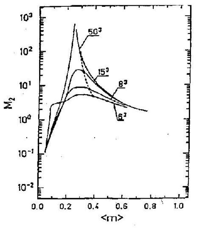
Figure 1: Second moment of the size distribution (see campi-here for a precise definition) as a function of the average cluster multiplicity for the three-dimensional percolation model for different lattice sizes. Figure is taken from perco .

Finite size effects have other consequences on the distribution than the simple smoothing of the transition. It has been shown on different model calculations that the presence of conservation constraints as well as the use of different event sorting procedures can sensibly distort the fluctuation observables. To give a simple example, the presence of a peak in the largest fragment’s size fluctuation as a function of the energy deposit is trivially produced by the baryon number conservation constraint which forces this fluctuation to decrease with increasing average multiplicityelliott . In the case of a genuine critical behavior as for the percolation model, the fact of sorting events according to the percolation parameter $p$ or according to some other correlated observable, as for instance the total cluster multiplicity, modifieselliott ; aladin the behavior of $m_{2}$, $\gamma_{2}$, and all other related momentscampi-here measuring the fluctuation properties of the system. All these effects can be understood in the general framework of the non- equivalence of statistical ensembles for finite systems, which we will discuss in the next chapter.

1.2 Thermal invariance properties

Another problem when trying to connect a fluctuation peak to a phase transition or a critical behavior in a finite system is given by the possible existence of thermodynamic ambiguities. It has been observed by different independent works that in the framework of equilibrium fragmentation models the fluctuation behavior is qualitatively independent of the break up density raduta ; richert ; dasgupta ; prl99 . An example is given in Figure 2, which gives the second moment of the charge ($S_{2}=M_{2}-M_{1}^{2}$) and of the energy ($C_{v}$) distribution as a function of temperature in the Lattice Gas model for different break-up densities in the subcritical regime.

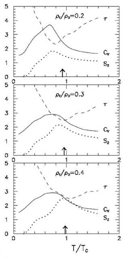
Figure 2: Second moment of the charge ($S_{2}$) and of the energy ($C_{v}$) distribution as a function of temperature in the Lattice Gas model for different densities for a system of linear dimension L=7. Arrows: first order transition temperature in the thermodynamic limit. Figure taken from ref.dasgupta .

A peak in the fluctuation observables can be seen at all densities, at a temperature which is systematically below the critical temperature of the system and close to the first order transition temperature in the thermodynamic limit. A similar behavior has been observed in different fluctuation observables and also at supercritical densities along the Kertesz percolation line, where the system does not present any phase transition. Table 1 gives, as a function of the lattice size, the inverse temperature at which the variable $S_{2}$ shows a maximum in the three-dimensional IMFM modelrichert at different densities.

Table 1: Inverse temperature at which the second moment $S_{2}=M_{2}-M_{1}^{2}$ is maximal for different densities and lattice sizes in the three-dimensional IMFM model. Taken from ref.richert

L	$\beta_{c}(\rho=.3)$	$\beta_{c}(\rho=.5)$	$\beta_{c}(\rho=.7)$
10	.2560(5)	.225(3)	.194(2)
16	.2440(2)	.2230(5)	.1984(2)
20	.23960(10)	.2227(4)	.1990(6)
24	.2367(3)	.2227(2)	.2005(6)

As a general statement, the fluctuation peak as well as the global scaling properties of the size distributionprl99 ; fisher in these models can be found along a curve in the $T(\rho)$ diagram passing through the thermodynamic critical point but extending in the subcritical as well as supercritical regioncampi-kertesz . The subcritical behavior can be understood as a finite size effect, when the correlation length, close to the first order transition point, becomes comparable to the linear size of the system, while the supercritical behavior is linked to the definition of clusters in dense and hot mediacampi-kertesz . For the subcritical region, a clusterization algorithm has been suggested to eliminate such behaviors in Ising simulationselliott-here . The possible pertinence of all these observations to experimental data is still a subject of debate, and essentially depends on the relationship between the measured clusters and the cluster definitions of the models.

Last but not least, the presence of different timescales in the reaction bonasera-here ; roy-here ; dorso-here and the dynamics of the fragmentation process may have important effects in the quantitative value of charge partition fluctuationsclaudio , as we will discuss in the last chapter.

For all these reasons, it is clear that the well documented presence of a fluctuation peak in the measured charge distributionstamain-here cannot be taken as such as a proof of a critical behavior and/or phase transition. In order to connect the fluctuation behaviour to a phase transition and to conclude on its order it is indispensable to compare with models and/or to quantify the fluctuation peak.

2 Theory

2.1 Fluctuations and constraints

It is clear that fluctuations on a given observable $A$ will be suppressed if a constraint is applied to a variable correlated to $A$. This trivial fact has a deep thermodynamic meaning and is linked to the non equivalence of statistical ensembles in finite systemsinequivalence . Indeed the basic statistical relation between a fluctuation and the associated susceptibility eq.(7) is only valid in the ensemble in which the fluctuations of $A$ are such as to maximise the total entropy, under the constraint of $\langle A\rangle$ (”canonical” ensemble). The thermodynamics in the ensemble where the generic observable $A$ is controlled event by event (”microcanonical” ensemble), or in the ensemble where $\sigma_{A}$ is externally fixed (”gaussian” ensemblechalla ) is a perfectly defined statistical problem, but the thermodynamic relationships have to be explicitly worked outnoi . As an example we show in Figure 3 the correlation between the size of the largest cluster $A_{big}$ and the total energy in the isobar Lattice Gas modelnoi at the transition temperature. The presence of two energy solutions at the same temperature and pressure clearly shows that the transition is in this case first orderlopez-here . The $A_{big}$ fluctuation properties are very different in the canonical ensemble (left part) and in the microcanonical ensemble (right part) at the same (average) total energy. Because of the important correlation between the total energy and the fragmentation partition, fragment size fluctuations can be compared only for samples with comparable widths of the energy distribution.

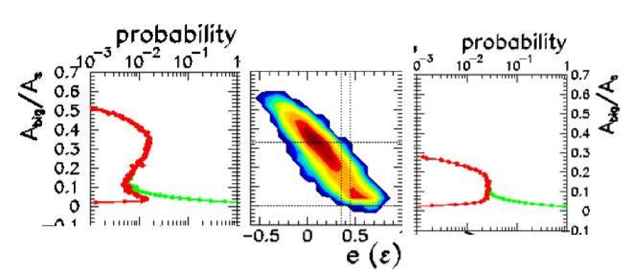
Figure 3: Center: correlation between the largest fragment’s size and the total energy in the isobar Lattice Gas model close to the transition temperature, for a system of 216 particles. Left side: projection over the $A_{big}$ direction. Right side: same as the left side, but only events within a narrow energy interval around the average energy have been retained.

From the experimental viewpoint, different constraints apply to fragmentation data and have to be taken into account. Apart from the sorting conditionstamain-here , the collisional dynamics can also give important constraints to the fragmentation pattern ($e.g.$ flows, deformation in r-space and p-space). This means that fluctuations have to be compared with calculations performed in the statistical ensemble corresponding to the pertinent experimental constraintsbotvina-here .

2.2 Fluctuations and susceptibilities

In the last subsection we have stated that a connection between a fluctuation and the associated susceptibility can always be in principle worked out if the constraints acting on the observable are known. In the case of sharp constraints ($e.g.$ fixed total mass, charge, deposited energy), the connection between the fluctuation on a variable correlated to the constraint ($e.g.$ size or charge of the largest fragment, configurational energy) and the associated susceptibility are in many cases analyticallebowitz ; npa99 ; gros . If a conservation constraint $A=A_{1}+A_{2}=cst$ applies and the system can be splitted in two statistically independent components such that $W(A)=W(A_{1})W(A_{2})$, then the partial fluctuations are linked to the total susceptibility by

$$\frac{\chi_{1}}{\chi}=1-\frac{\sigma^{2}_{1}}{\sigma^{2}_{ref}},$$ (8)

where $\chi_{i}^{-1}=\partial^{2}_{A_{i}}W_{i}$, $\sigma^{2}_{ref}$ is the fluctuation of $A_{1}$ in the ensemble where only the average value $\langle A\rangle$ is constrained, and we have approximated the distribution of $A_{1}$ with a gaussiannoi . The case of the total energy constraint has been particularly studied in the literature. Indeed the total energy deposit can be (approximatelyviola-here ) measured event by event in $4\pi$ experiments, allowing to experimentally construct a microcanonical ensemble by sorting. For classical systems with momentum independent interactions the potential energy fluctuation $\sigma^{2}_{I}$ at a fixed total energy is linked to the total microcanonical heat capacity by

$$\frac{C_{k}}{C}=1-\frac{\sigma^{2}_{k}}{\sigma^{2}_{can}},$$ (9)

where $C_{k}$,$C$ are the kinetic and total heat capacity, $\sigma^{2}_{k}=\sigma^{2}_{I}$ and $\sigma^{2}_{can}=c_{k}T^{2}$ is the kinetic energy fluctuation in the canonical ensemble. Apart from the microstate equi-probability inherent to all statistical calculations, the above formula is obtained in the saddle point approximation for the partial energy distributions. The contribution of non gaussian tails can be also analytically worked outnpa99 and has been found to be negligible in all theoretical as well as experimental data samples analyzed so farnoi . An exemple of the quality of the approximation is given in Figure 4 which gives the temperature, normalized potential energy fluctuation and heat capacity in the isobar Lattice Gas model for a system of 108 particles.

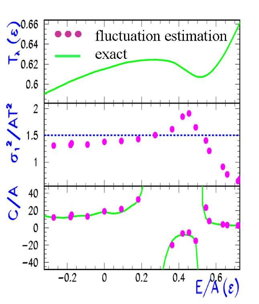
Figure 4: Temperature, normalized binding energy fluctuation and heat capacity in the microcanonical isobar Lattice Gas model as a function of the total energy for a system of 108 particles. In the lower panel the heat capacity estimated from fluctuations via eq.(9) (dots) is compared to the exact expression from the entropy curvature (line). Figure is taken from europhys .

3 Experiment

3.1 Effect of the sorting variable

In this section we turn to compare different sets of experimental data available in the literature. A special attention has been paid by different collaborations to the largest fragment fluctuation $\sigma_{m}$ eq.(3) and to the $\gamma_{2}$ observable eq.(2)aladin ; ags1 ; ags2 ; ags3 ; eos ; multics . For all data sets of comparable total size these observables, as well as the others we will show in the next subsections, show a well defined peak at comparable values of the chosen sorting variable. This is an important and non trivial result considering that data are taken with different apparata and the multifragmenting systems are obtained with very different reaction mechanisms. The effect of the sorting variable is explored in table 2, that gives the maximum value of $\gamma_{2}$ and $\sigma_{m}$ with different data sets sorted in bins of the total measured bound charge $Z_{bound}$, total measured charged particles multiplicity $m$, or calorimetric excitation energyviola-here .

Table 2: Maximum $\gamma_{2}$ and $\sigma_{m}$ values measured in the break up of a $Au$ system within different data sets sorted in $Z_{bound}$, total multiplicity ($m$) or calorimetric excitation energy ($\epsilon^{*}$). Different values for the same case denote different bombarding energies. Values taken from refs.aladin ; elliott ; ags1 ; ags2 ; ags3 ; eos ; multics

. $\gamma_{2}$aladin $\gamma_{2}$ags1 ; ags2 ; ags3 $\gamma_{2}$eos ; elliott $\gamma_{2}$multics $\sigma_{m}$eos $\sigma_{m}$multics $Z_{bound}$ 1.4 1.3 m 1.85 3.2 2.23 .15 1.85 2.5 $\epsilon^{*}$ 3.7 2.5 .12 .14

Even if the systematics should certainly be completed and errors should definitely be evaluated, we can observe from table 2 that different data sets show a reasonable agreement when the same sorting is employed.

We can also note that a higher $\gamma_{2}$ is systematically obtained when data are analyzed in bins of total charge multiplicity, with respect to a sorting in $Z_{bound}$. This can be qualitatively understood if we recall that $\gamma_{2}$ measures the variance of the charge bound in fragments, and this quantity is obviously strongly correlated with $Z_{bound}$ and loosely correlated with $m$. The calorimetric excitation energy sorting leads to comparable results to the multiplicity sorting. The value of $\gamma_{2}$ is slightly increased, which may be explained by a reduced correlation of $\epsilon^{*}$ with respect to $m$ with the total fragment charge, since the excitation energy contains the extra information of the kinetic energy of the fragments. However the effect goes in the opposite direction as the fluctuation of $Z_{m}$ is concerned. A detailed study of the correlation coefficient between the considered observables and the sorting variables is needed to fully understand thess trends. It is also possible that the fluctuations obtained with these two sortings may be compatible within error bars, which stresses the importance of an analysis of errors.

The fluctuation values appear to be largely independent of the reaction mechanism and incident energyaladin ; ags1 ; ags3 . The only exception is the value $\gamma_{2}\approx 2.5$ obtained from emulsion data in ref.ags2 , which is significantly higher than the values obtained at the other bombarding energies for the same system. Such anomaly might be due to the presence of fission events that have been excluded in the other analysesags1 ; ags3 . The independence on the incident energy tends to show that the fragmentation process is essentially statistical.

3.2 Effect of the system size

The effect of the system size is further analyzed in table 3. All presented data are sorted in bins of calorimetric excitation energy.

Table 3: Maximum $\gamma_{2}$, $\Sigma^{2}_{m}$ and $\sigma_{m}$ values measured within different data sets for various system sizes $Z_{0}$. Different values for the same case denote different targets. Values taken from refs.eos ; nimrod ; multics

. $<Z_{0}>$ $\gamma_{2}$eos ; nimrod ; multics $\Sigma^{2}_{m}$eos ; nimrod ; multics $\sigma_{m}$eos ; nimrod ; multics 76 2.5 1.49 0.14 59 3.7 0.85 0.12 43 2.4 0.73 0.13 27 1.75 0.39 0.125 16 1.19 0.22 0.114 1.17 0.22 0.114 1.16 0.22 0.114

The fluctuation properties of quasi-projectile decay appear to be largely independent of the target. This well known behavior at relativistic energyaladin appears confirmed in the case of the Nimrod experimentnimrod which was performed with a beam energy as low as 47 MeV/A. This suggests that a quasi-projectile emission source can be extractedtamain-here in spite of the important midrapidity contribution in the Fermi energy regimeroy-here .

From table 3 we can also see that $\Sigma^{2}_{m}$ decrease monotonically with the system mass. The evolution with the system size, at least in the size range analyzed, appears as a simple scaling behavior as shown by the fact that the normalization to the source size in $\sigma_{m}$ makes the fluctuation almost independent of the size. Similar conclusions can be drawn concerning the $\gamma_{2}$ observable, even if the behavior for the heaviest sources is less clear. This interesting scaling behavior should be confirmed using hyperscaling techniquescampi-here .

To conclude, we have seen that fluctuations can vary of a factor two changing the sorting variable. This stresses the need of confronting the experimental data with statistical predictions containing the same constraints, i.e. performed in the adapted statistical ensemble. Interesting enough, when the same sorting is adopted the different available data sets agree within $\approx$ 15% both in the value of the peak and in the position where the peak is observed. More data are needed to confirm these trends.

3.3 Configurational energy fluctuations

One of the most interesting aspects of studying fluctuation observables, is their possible connection with a susceptibility or a heat capacity via eq.(9). Configurational energy fluctuations have been studied at length by the Multics collaborationplb ; palluto ; mich-last and by the Indra collaborationpalluto ; nicolas ; lopez ; bernard on Au sources. The observable used in these studies is an estimation of the energy stored in the configurational degrees of freedom at the time of fragment formation, defined as follows

$$E_{I} = \sum_{i=1}^{N_{imf}}Q\left(Z_{i}^{p},A_{i}^{p}\right)$$

$$+ \sum_{i=n,p,d,t,^{3}He,^{4}He}Q\left(Z_{i},A_{i}\right)M_{i}^{p}$$

$$+ V_{coul}\left(\left\{Z_{i}^{p}\right\},V_{FO}\right)$$

where $Q$ indicates the mass defects and $V_{coul}$ the coulomb energy. The measured fragment charges $Z_{i}$ and lcp multiplicities $M_{i}$ are corrected in each event to approximately account for secondary decay

$$Z_{i}^{p} = Z_{i}+\langle M^{ev}_{H}+2M^{ev}_{He}\rangle\frac{Z_{i}}{\sum_{i=1}^{N_{imf}}Z_{i}}$$ (11)

$$M_{i}^{p} = M_{i}-\langle M^{ev}_{i}\rangle$$ (12)

where $\langle M^{ev}_{i}\rangle$ is the estimated multiplicity of secondary emitted light charged particles for each calorimetric excitation energy bin.

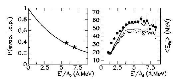
Figure 5: Left part: percentage of secondarily emitted light charged particles taken from correlation functions measurements (see ref.giuseppe-here ). Right part: total measured fragment kinetic energy (points) compared with Coulomb trajectories calculations where the volume is changed from $6V_{0}$ to $3V_{0}$. Both quantities are plotted as a function of the calorimetric excitation energy. Figure is taken from palluto .

Three quantities need to be estimated in each excitation energy bin to compute $E_{I}$

1. The freeze out volume $V_{FO}$ which determines the total Coulomb energy. Its average value is deduced from the measured fragment kinetic energies through Coulomb trajectories calculations (see Figure 5, right part).

2. the average multiplicities of secondarily emitted particles $\langle M^{ev}_{lcp}\rangle$ to account for side feeding effects. They are deduced from fragment-particle correlation functions (see Figure 5, left part).

3. the isotopic content $A_{i}^{p}/Z_{i}^{p}$ of primary fragments. It is assumed that it is equal to the isotopic content of the fragmenting system. This quantity allows in turn to determine the number of free neutrons at freeze out from baryon number conservation.

A general protocol has been proposed to minimize the spurious fluctuations due to the implementation of this missing informationpalluto . The resulting fluctuation of $E_{I}$ $\sigma^{2}_{I}=\sigma^{2}_{k}$ is shown for different Multics data in figure 6. The temperature has been estimated alternatively using isotopic thermometers or solving the kinetic equation of state and comes out to be in good agreementmich-last with the general temperature systematics natowiz-here (around 4.5 MeV in the fragmentation region).

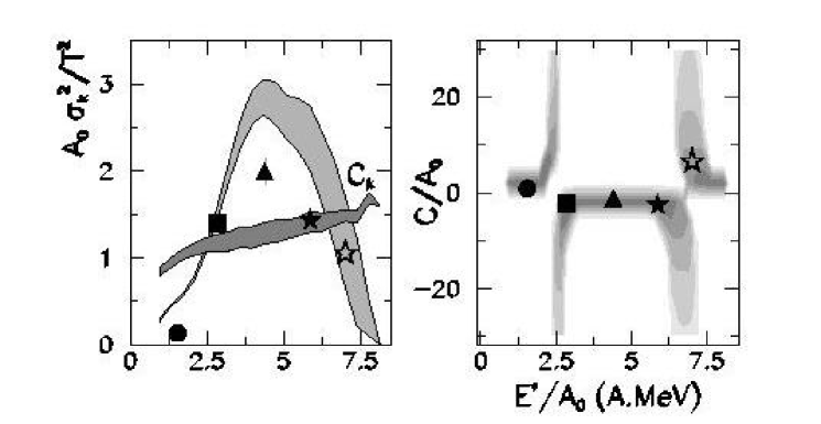
Figure 6: Left side: normalized fluctuation of $E_{I}$ and estimated $C_{k}$ (see text) as a function of the calorimetric excitation energy. Grey zone: peripheral 35A.MeV Au+Au collisions. Symbols: central Au+C, Au+Cu, Au+Au at 25 and 35 A.MeV. Right side: heat capacity from eq.9. Figure is taken from mich-last .

Similar to the other fluctuation observables, configurational energy fluctuations show a well pronounced peak at an excitation energy around 5 A.MeV. This general feature is apparent in Multicsmich-last , Indrabernard , Isislefort and Nimrodnimrod data. The only exception is EOS datasrivastava where this fluctuation appears monotonically decreasing.

In the hypothesis of thermal equilibrium at the freeze out configuration this fluctuation is a measurement of the heat capacity according to eq.(9). The value expected for this fluctuation in the canonical ensemble can be written as $\sigma^{2}_{can}=c_{k}T^{2}$. The kinetic heat capacity $c_{k}$ is calculated from the measured fragment yieldspalluto . We can see that the fluctuation peak overcomes the upper classical limit $c_{k}=3/2$ suggesting a negative heat capacity as expected in a first order phase transition analyzed in the microcanonical ensemblechomaz-here ; gross-here .

The same analysis performed on Indra data of central Xe+Sn collisions at different bombarding energies leads to compatible temperatures and volumes and a fluctuation estimation that agrees within 25% with the presented Multics resultspalluto , as shown for the 32 A.MeV data in figure 7 (upper part). In the absence of isotopic resolution for fragments, Coulomb repulsion cannot be distinguished from a radial collective expansion due to a possible initial compression. If an important radial flow component is assumed for these central collisions, data can also be compatible with a bigger freeze out volume (lower part of the figure) leading to a shift of the abnormal fluctuation behavior towards lower energy. This volume/flow ambiguity in central collisions can only be solved with third generation multidetectorsleneindre-here .

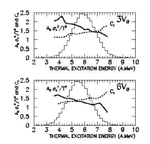
Figure 7: Normalized fluctuation and kinetic heat capacity (stars) for 32 A.MeV Xe+Sn central collisions measured by the INDRA collaboration as a function of the calorimetric excitation energy with two different hypothesis on the freeze out volume. The histogram gives the event distribution. Figure is taken from nicolas ; palluto .

Indra data on the same Au quasi-projectile analyzed by the Multics collaboration lead to a fluctuation measurement about 40% lower, see figure 8. This difference is tentatively explained as an effect of emission from the neck which leads to a reduced occupation of the available phase spacebernard .

Recent Nimrod datanimrod on the fragmentation of a much lighter system show a similar value for the energy corresponding to the fluctuation peak, but fluctuation a factor 10 lower than for Multics data, as shown in figure 9. If we consider the global fluctuation $<A_{0}>\sigma^{2}_{k}$ without the normalization to the estimated temperature, this factor is reduced to about a factor 4. These results go in the same direction as the general behavior of $\Sigma^{2}_{m}$ that we have analyzed in section 3.2. Recall that the fluctuation of the biggest fragment for the quasi-Au sourcemultics is a factor 6.8 higher than for the quasi-Arnimrod . This fluctuation reduction seems then to be a general feature of light systems fragmentation and has been tentatively explained as an effect of the higher temperature that light systems can sustainnimrod . In this interpretation, a higher temperature region of the phase diagram, possibly above the critical point, is explored in the fragmentation of light systems, and the first order phase transition observed in heavy nuclei becomes a smooth cross over.

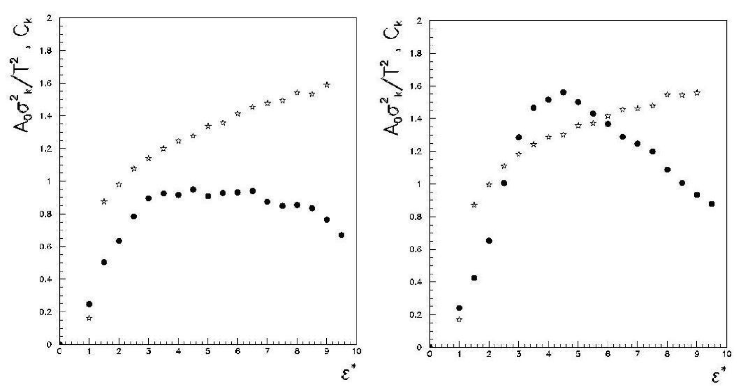
Figure 8: Normalized fluctuation and kinetic heat capacity (stars) for 80 A.MeV Au+Au peripheral collisions measured by the INDRA and ALADIN collaboration as a function of the calorimetric excitation energy, for all quasi-projectile events (left side) and after subtraction of events elongated along the beam axis (right side). Figure is taken from bernard .

Figure 9: Normalized fluctuation and kinetic heat capacity for 47 A.MeV Argon quasi-projectiles on different targets measured by the NIMROD collaboration as a function of the calorimetric excitation energy. Figure is taken from nimrod .

As a general remark, the configurational energy fluctuation signal is a very interesting one due to its possible connection with a heat capacity, but it is also a very indirect and fragile experimental signal which needs precise calorimetric measurements, a careful data analysis, extensive simulations to assess the effect of the different hypotheses in the event sorting and reconstruction procedure. Moreover the different techniques to exclude or minimize preequilibrium and neck emission seem to have a strong influence in the absolute value of fluctuations.

The evaluation of systematic errors in fluctuation measurements is necessary to achieve a quantitative estimation of fluctuations: some first encouraging results in this direction have been presented in ref.mich-last . The confirmation (or infirmation) of the fluctuation enhancement is certainly one of the most important challenges of the field in the next years with third generations multidetectors.

4 Open questions

The possibility of accessing a thermodynamic information on the nuclear phase diagram from measured fragment properties entirely relies on the representation of the system at the freeze out stage as an ideal gas of fragmentsbotvina-here in thermal equilibrium. This is true for fluctuation observables as well as for all other thermodynamic analysesnatowiz-here ; elliott-here . This is an important conceptual point which is presently largely debated in the heavy ion community.

A first open question concerns the structure of the systems at the freeze out stage, i.e. at the time when fragments decouple from each other. Contrary to the ultrarelativistic regimerandrup-here , we do not expect much difference between the chemical and kinetic decoupling times due to the small collective motions implied in these low energy collisions. We can therefore speak at least in a first approximation of a single freeze out time. If at this time the system is still relatively dense, the cluster properties may be very different from the ones asymptotically measured, and the question arisescampi-kertesz whether the energetic information measured on ground state properties can be taken backward in time up to the freeze out. Calculations from classical molecular dynamicscampi show that the ground state Q-value is a very bad approximation of the interaction energy of Hill clusters in dense systems. This is due both to the deformation of clusters when recognized in a dense medium through the Hill algorithm, and to the interaction energy among clusters in dense configurations where clusters surfaces touch. As a consequence, comparable fluctuations are obtained in the subcritical and supercritical region of the Lennard-Jones phase diagram. This result is shown in fig.10.

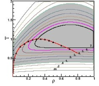
Figure 10: Phase diagram of 64 Lennard Jones particles confined in a box. Filled triangles give the coexistence border. Isocontours give values of normalized fluctuations $\sigma^{2}_{k}/\sigma^{2}_{can}$ calculated from the ground state Q value of clusters defined with the Hill algorithm. Figure is taken from campi .

Calculations in a similar model, the Lattice Gas model, show that even in the supercritical regime the correct fluctuation behavior can be obtained if both the total energy and the interaction energy are consistently estimated with the same approximate algorithm as it is done in the experimental data analysistracking . Indeed the high value of the estimated configurational energy $Q$ fluctuations is essentially due to the spurious fluctuation of the total energy $E_{K}+E_{I}$ obtained when $E_{I}$ is estimated through $Q$; such an effect is eliminated if data are analyzed in bins of $E_{K}+Q$. This calculation is shown in fig.11.

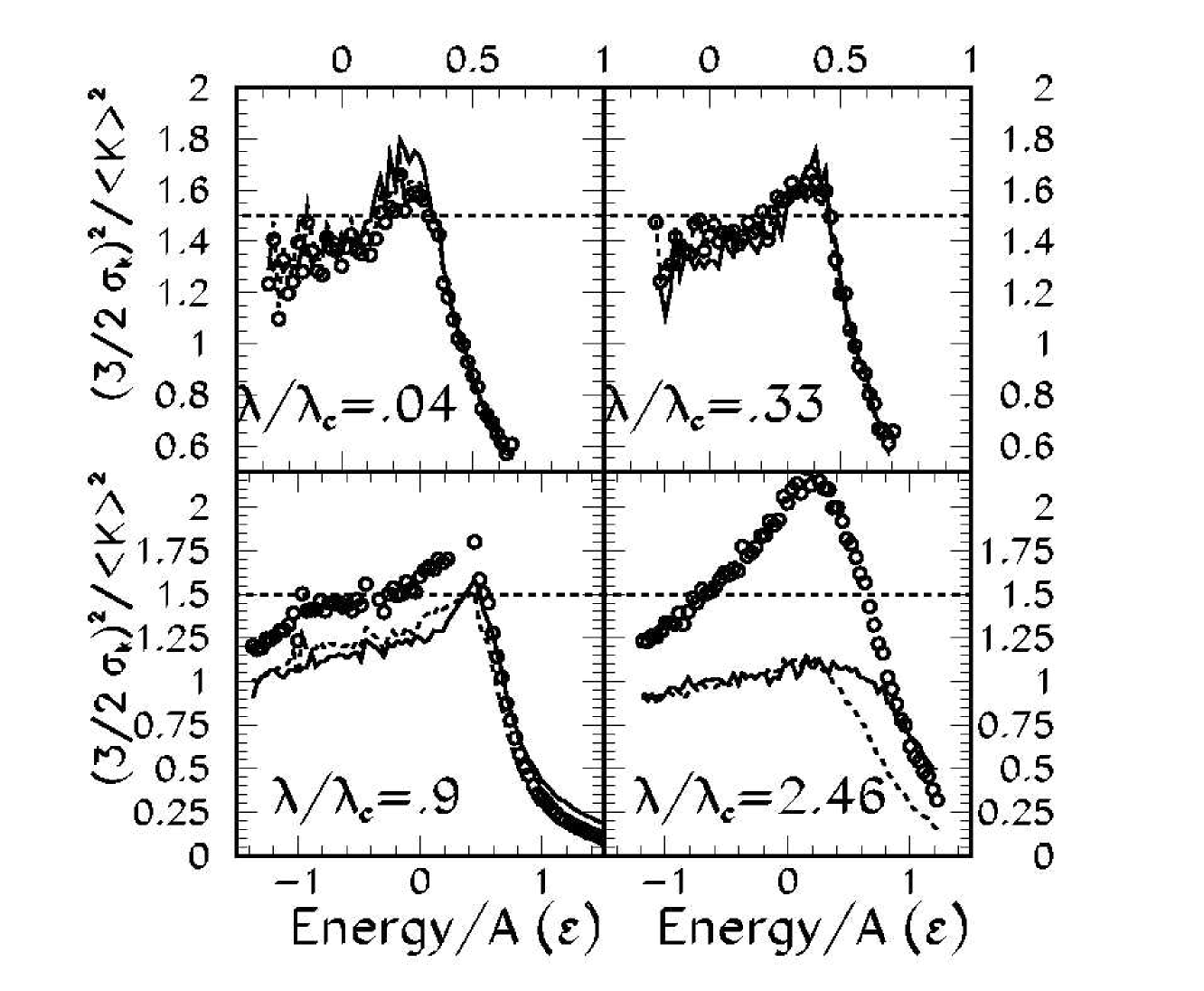
Figure 11: Normalized fluctuations $\sigma^{2}_{k}/T^{2}$ as a function of energy for a system of 216 Lattice Gas particles in the isobar ensemble at different pressures. Full lines: exact results. Symbols: estimation from the ground state Q value of Coniglio-Klein clusters. Dashed lines: as the symbols, but data are sampled in bins of energy reconstructed from cluster kinetic energies and sizes. $\lambda_{c}$ gives the critical pressure. Figure is taken from tracking .

A second related question which needs further work is the relevance of the equilibrium assumption at freeze out. Molecular dynamics models applied to study the time evolution of the reactionclaudio ; ariel ; akira ; aichelin predict that the decoupling between fragment degrees of freedom (freeze out) occurs very rapidly during the reaction. At this stage however the configuration is considerably diluted due to the early presence of collective motionsclaudio ; dorso-here . An example taken from classical molecular dynamics for an initially equilibrated compact configuration freely evolving in the vacuum, is shown in fig.12. At this reaction stage cluster energies may be well approximated (within a side feeding correction) by their asymptotically measured values, but it is not clear whether this configuration can correspond to an equilibrium, more precisely whether the hypothesis of equiprobability of the different charge partitions holds.

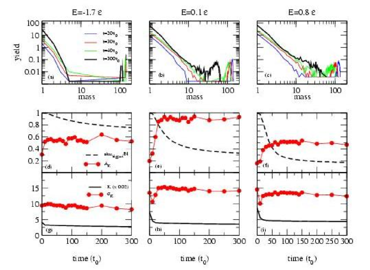
Figure 12: Time evolution of a Lennard Jones system initially confined in a dense supercritical configuration and freely expanding in the vacuum at different total energies. Upper part: MST fragment size distribution at different times. Lower part: average kinetic energy (full lines), total (lower symbols) and normalized (upper symbols) kinetic energy fluctuations, and size of the largest MST cluster (dashed lines). Abnormal fluctuations in these units correspond to $A_{k}>\approx 0.7$. Figure is taken from ariel .

5 Conclusions and outlooks

In this paper we have presented a short review of the experimental as well as theoretical studies of fluctuation observables of fragments produced in a multifragmentation heavy ion reaction. The aim of these studies is the understanding of the nature of the nuclear fragmentation transition as well as the thermodynamic characterization of the finite temperature nuclear phase diagram. This vast and ambitious program is still in its infancy. Many promising results already exist, but the analyses are not yet conclusive and need to be intensively pursued in the future.

The nuclear fragmentation phenomenon, well documented by a series of independent experimentstamain-here , presents many features compatible with a critical phenomenoncampi-here or a phase transitionelliott-here ; lopez-here . Only a careful study of fluctuation properties will allow to discriminate between the different scenarii. Even more important, the phase diagram of finite nuclei is theoretically expected to present an anomalous thermodynamicsgross-here ; chomaz-here which should be characteristic of any non extensive system undergoing first order phase transitions in the thermodynamic limit. Once the difficulties linked to the imperfect detection and sorting ambiguities will be overcome, fluctuation observables will be a unique tool to quantitatively study this new thermodynamics with its interdisciplinary applicationsgross-here ; chomaz-here ; pleimling .

From the theoretical point of view, the theoretical connections between fluctuations and susceptibilities in the different statistical ensembles are well established, and the different experimental contraints can be consistently adressed by the theory. However, the evaluation of a thermodynamics for a clusterized system opens the difficult theoretical problem of cluster definition in dense quantum media. To produce quantitative estimations of measurable fluctuation observables the pertinence of classical models has to be checked through detailed comparisons with microscopicakira and macroscopicbotvina-here nuclear models.

On the experimental side, multiplicities and size fluctuations agree reasonably well if comparable size fragmenting systems are studied, even if the effect of the system size has to be clarified. Configurational energy fluctuations are especially interesting because of their possible connection with a heat capacity measurement. The methodology to extract such fluctuations from fragmentation data is presently under debate, in particular a careful analysis of systematic errors is presently undertakenmich-last . From a more conceptual point of view, the influence of the different time scales in the reaction dynamics has to be clarified. Configurational energy fluctuations may be subject to strong ambiguities since they use information from all the particles of the event, and this information is integrated over the whole reaction dynamics. In this respect, an interesting complementary observable may be given by fluctuation of the heaviest cluster sizelopez-here ; gros .

To solve the existing ambiguities we need full comparisons with a well defined protocol and consistency checks between different data sets. The simultaneous measurement of fragments mass and charge on a $4\pi$ geometryleneindre-here will be essential to measure the basic variable of any thermodynamic study, namely the deposited energy. No definitive conclusion about the occurrence of a thermodynamic phase transition and its order can be drawn without this detection upgrade.

References

- (1) G.Bertsch, P.J.Siemens, Phys. Lett. B 126 (1983)9.
- (2) H.Muller and B.Serot, Phys. Rev. C52 (1995) 2072.
- (3) C.Ducoin et al, nucl-th/0512029.
- (4) G.Bizard et al, Physics Letters B 208 (1993) 162.
- (5) A.Schuttauf et al, Nuclear Physics A 607 (1996) 457.
- (6) T.Beaulieu et al, Physical Review C 64 (2001) 064604.
- (7) B.Tamain, contribution to this book.
- (8) X.Campi, Physics Letters B 208 (1988) 351.
- (9) J.B.Elliott et al, contribution to this book.
- (10) J.Elliott et al, Physical Review C 62 (2000) 064603.
- (11) Y.G.Ma, contribution to this book.
- (12) Al.Raduta et al, Phys.Rev. C 65(2002)034606.
- (13) J.Carmona et al, Nuclear Physics A 643 (1998) 115.
- (14) J.Pan et al, Physical Review Letters 80 (1998) 1182.
- (15) Ph.Chomaz, F.Gulminelli, Physical Review Letters 82 (1999) 1402.
- (16) F.Gulminelli et al, Phys.Rev.C 65(2002) 051601.
- (17) N.Sator, Phys.Rep. 376 (2003) 1.
- (18) A.Bonasera et al, contribution to this book.
- (19) M.Di Toro et al, contribution to this book.
- (20) C.Dorso, contribution to this book.
- (21) P.Balenzuela et al, Physical Review C 66 (2002) 024613.
- (22) F.Gulminelli et al, Physical Review E 68 (2003) 026120.
- (23) M.S.Challa, J.H.Hetherington, Phys.Rev.Lett. 60 (1988) 77.
- (24) F.Gulminelli, Ann. Phys. Fr. 29 (2004)6.
- (25) O.Lopez and M.F.Rivet, contribution to this book.
- (26) A.Botvina, contribution to this book.
- (27) J.L.Lebowitz et al, Physical Review 153 (1967) 250.
- (28) F.Gulminelli,Ph.Chomaz ,Nuclear Physics A 647 (1999) 153.
- (29) F.Gulminelli,Ph.Chomaz, Physical Review C 71 (2005) 054607.
- (30) V.Viola and R.Bougault, contribution to this book.
- (31) F.Gulminelli, Ph.Chomaz and V.Duflot, Europhys.Lett.50 (2000) 434.
- (32) P.L.Jain et al, Physical Review C 50 (1994) 1085.
- (33) M.I.Adamovitch et al, European Journal of Physics A 1 (1998) 77.
- (34) D.Kudzia et al, Physical Review C 68 (2003) 054903.
- (35) J.B.Elliott et al, Physical Review C 67 (2003) 024609.
- (36) A.Bonasera et al, La Rivista del Nuovo Cimento 23 (2000) 1; M.D’Agostino, private communication.
- (37) Y.G.Ma et al, Nucl.Phys. A 749 (2005) 106; Y.G.Ma, private communication.
- (38) M.D’Agostino et al, Physics Letters B 473 (2000) 219.
- (39) M.D’Agostino et al, Nuclear Physics A 699 (2002) 795.
- (40) M.D’Agostino et al, Nuclear Physics A 734 (2004) 512.
- (41) N.Leneindre, PhD, http://tel.ccsd.cnrs.fr/tel-0003741
- (42) O.Lopez et al, proceedings of the IWM meeting, Caen, 2003
- (43) M.Pichon et al, nucl-ex/0602003 and PhD, http://tel.ccsd.cnrs.fr/tel-0007451.
- (44) J.Natowiz and K.H.Schmidt, contribution to this book.
- (45) T.Lefort and V.Viola, private communication.
- (46) B.K.Srivastava et al., Phys.Rev. C65 (2002) 054617.
- (47) G.Verde et al, contribution to this book.
- (48) P.Chomaz, contribution to this book.
- (49) D.Gross, contribution to this book.
- (50) J.Randrup and I.Mishustin, contribution to this book.
- (51) X.Campi et al, Phys.Rev.C 71 (2005) 41601.
- (52) F.Gulminelli, Ph.Chomaz, M.D’Agostino,Phys.Rev. C72 (2005) 064618.
- (53) A.Chernomoretz et al, Physical Review C 69 (2004) 034610.
- (54) A.Ono, H.Horiuchi, Progr. Part. Nucl. Phys. 53 (2004) 501.
- (55) A.D.Sood, R.K.Puri, J.Aichelin, Phys.Lett. 594 (2004) 260.
- (56) H.Behringer et al, J.Phys.A 38 (2005) 973.
- (57) N.Leneindre et al., contribution to this book.