A method for determining event-by-event elliptic flow fluctuations
based on the first-order event plane in heavy-ion collisions

Abstract

A new method is presented for determining event-by-event fluctuations of elliptic flow, $v_{2}$, using first-order event planes. By studying the event-by-event distributions of $v_{2}$ observables and first-order event-plane observables, average flow $\langle v_{2}\rangle$ and event-by-event flow fluctuations can be separately determined, making appropriate allowance for the effects of finite multiplicity and non-flow. The method has been tested with Monte Carlo simulations. The connection between flow fluctuations and fluctuations of the initial-state participant eccentricity is discussed.

I Introduction

In heavy-ion collisions, the azimuthal distributions of emitted particles can be decomposed with a Fourier expansion Methods :

$$\frac{dN}{d\varphi}=\frac{1}{2\pi}\{1+\sum_{n=1}^{\infty}2v_{n}\cos n(\varphi-\Psi_{\rm RP})\},$$ (1)

where $\varphi$ denotes the azimuthal angle of the particle and $\Psi_{\rm RP}$ is the reaction plane azimuth (defined by the impact parameter vector). The Fourier coefficients,

$$v_{n}=\langle\cos n(\varphi-\Psi_{\rm RP})\rangle\,,$$ (2)

are referred to as anisotropic flow of the $n^{\rm th}$ harmonic. The second harmonic, elliptic flow, carries information on the early stage of heavy-ion collisions, and has been extensively studied. Event-by-event flow fluctuations STARlongFlow130 ; STARlongFlow200 ; MillerSnellings ; Mrow-Shuryak ; Phobos06 ; SorensenQM06 are of considerable interest as they must be sensitive to the physics of the very early stages of the collision, and because any fluctuation observable has potential relevance for phase transition phenomena. Understanding flow fluctuations would also greatly improve anisotropic flow measurements that are currently dominated by systematic uncertainties in which flow fluctuations play a crucial role. At fixed centrality, initial-state fluctuations in the spatial anisotropy of the participant zone will cause flow fluctuations. In addition to this inevitable source of fluctuations, there might be additional fluctuation contributions that could offer unique insights into dynamical details of the collision process at very early times (1 fm$/c$ and earlier) Mrow-Shuryak . The large observed elliptic flow at the Relativistic Heavy Ion Collider (RHIC) points to a very short thermal equilibration time in the framework of hydrodynamic models. This puzzling feature calls for further investigation and could have alternative explanations or might be explained by exotic phenomena Mrow93-97 ; KovTuchin02 ; KNV03 ; Shuryak03 . Improved methods to experimentally determine flow fluctuations would be an important step towards addressing some or all of the open issues discussed above.

Fluctuations in the shape of the initial participant region, and in particular, in the orientation of the region’s principal axes relative to the direction of the impact parameter, lead to a non-trivial picture of anisotropic flow. In this picture, the apparent flow at mid-rapidity might be different in direction and magnitude from the real flow as measured with respect to the reaction plane. The method proposed in this paper is sensitive to such a difference, and allows fluctuations in the orientation of the principal axes of the participant region to be measured.

RHIC data hold much promise for the purpose of understanding elliptic flow fluctuations, since $v_{2}$ is large, while the statistical noise arising from finite multiplicity, that tends to obscure the dynamical fluctuations of interest, is smaller than at lower energies. Most flow analyses at RHIC to date have relied on the second-order event plane, whereas in the present study, a case is presented for utilizing the first-order event plane to determine the mean elliptic flow, and to isolate the sought-after dynamical fluctuations about that mean. In RHIC experiments, first-order event planes can be obtained, for example, via the ZDC-SMD (Zero Degree Calorimeter Shower Maximum Detector) ZDC or the Forward TPC FTPC-NIM of the STAR detector. In the scenario envisaged here, the fluctuating anisotropies are based on measurements near mid-rapidity, while the first-order event plane determination utilizes detectors that are far removed in rapidity. Consequently, non-flow effects (defined as azimuthal correlations that may contribute to $v_{n}$ measurements, but which are unrelated to the reaction plane orientation, or more generally, are unrelated to the initial geometry of the system) are believed to be negligible using this method STARv1at62 .

II Technique

With two independent first-order event planes $\psi_{a}$ and $\psi_{b}$, elliptic flow can be determined with the help of the relations

$$v_{2}^{\rm obs} = \langle\cos(2\varphi-\psi_{a}-\psi_{b})\rangle$$ (3)

$$= \langle\cos(2\varphi-2\Psi_{\rm RP})\rangle\,\langle\cos(2\Psi_{\rm RP}-\psi_{a}-\psi_{b})\rangle$$

$$= v_{2}\,\langle\cos(\psi_{a}-\psi_{b})\rangle\,,$$

where the last factor, $\langle\cos(\psi_{a}-\psi_{b})\rangle=\langle\cos(\psi_{a}-\Psi_{\rm RP})\rangle\langle\cos(\psi_{b}-\Psi_{\rm RP})\rangle$ is the product of the two first-order event plane resolutions Methods . The above is based on the assumptions that the two event planes are independent, and that the distributions of $\psi_{a}$ and $\psi_{b}$ with respect to the true reaction plane are symmetric.

We introduce two event-by-event quantities

$$c_{2;k} = \langle\cos 2(\varphi-\Psi_{{\rm RP};k})\rangle$$ (4)

$$s_{2;k} = \langle\sin 2(\varphi-\Psi_{{\rm RP};k})\rangle\,,$$ (5)

where index $k$ denotes the $k^{\rm th}$ event and the average is taken over all particles in that event. Using the equality

$$\cos(2\varphi-\psi_{a;k}-\psi_{b;k}) = \cos[2(\varphi-\Psi_{{\rm RP};k})-(\psi_{a;k}-\Psi_{{\rm RP};k})-(\psi_{b;k}-\Psi_{{\rm RP};k})]$$ (6)

$$= \cos 2(\varphi-\Psi_{{\rm RP};k})\,\cos(\Delta\psi_{a;k}+\Delta\psi_{b;k})+\sin 2(\varphi-\Psi_{{\rm RP};k})\,\sin(\Delta\psi_{a;k}+\Delta\psi_{b;k}),$$

where $\Delta\psi_{a;k}=\psi_{a;k}-\Psi_{{\rm RP};k}$ and $\Delta\psi_{b;k}=\psi_{b;k}-\Psi_{{\rm RP};k}$ (and a similar expression for $\sin(2\varphi-\psi_{a;k}-\psi_{b;k})$), and averaging over particles in the $k^{\rm th}$ event, one finds

$$c_{2;k}^{\rm obs} = c_{2;k}\cos(\Delta\psi_{a;k}+\Delta\psi_{b;k})+s_{2;k}\sin(\Delta\psi_{a;k}+\Delta\psi_{b;k})$$ (7)

$$s_{2;k}^{\rm obs} = s_{2;k}\cos(\Delta\psi_{a;k}+\Delta\psi_{b;k})-c_{2;k}\sin(\Delta\psi_{a;k}+\Delta\psi_{b;k})\,.$$ (8)

We further assume that the distribution of the first-order event planes $\{{\Delta\psi_{a;k}+\Delta\psi_{b;k}}$} is independent of distributions $\{{c_{2;k}}$} and $\{{s_{2;k}}$} . This assumption is usually not valid for second-order event planes, and this illustrates one of the advantages of the present approach. Assuming that $\{{\Delta\psi_{a;k}}$} and $\{{\Delta\psi_{b;k}}$} are both symmetric around zero and independent, the distributions $\{{\Delta\psi_{a;k}+\Delta\psi_{b;k}}$} and $\{{\Delta\psi_{a;k}-\Delta\psi_{b;k}\equiv\Delta\psi_{ab;k}}$} are identical. We discuss the validity of all of the above assumptions in more detail at the end of Section III.

From Eqs. (7) and (8) one can calculate the mean (now averaged over all events) and the mean square of $c_{2;k}^{\rm obs}$ and $s_{2;k}^{\rm obs}$  :

$$\langle c_{2;k}^{\rm obs}\rangle=\langle c_{2;k}\rangle\,\langle\cos\Delta\psi_{ab;k}\rangle=v_{2}\,\langle\cos\Delta\psi_{ab;k}\rangle\,,$$ (9)

$$\langle s_{2;k}^{\rm obs}\rangle=0\,,$$ (10)

$$\langle(c_{2;k}^{\rm obs})^{2}\rangle=\langle c_{2;k}^{2}\rangle\,\langle\cos^{2}\Delta\psi_{ab;k}\rangle+\langle s_{2;k}^{2}\rangle\,\langle\sin^{2}\Delta\psi_{ab;k}\rangle\,,$$ (11)

$$\langle(s_{2;k}^{\rm obs})^{2}\rangle=\langle c_{2;k}^{2}\rangle\,\langle\sin^{2}\Delta\psi_{ab;k}\rangle+\langle s_{2;k}^{2}\rangle\,\langle\cos^{2}\Delta\psi_{ab;k}\rangle\,.$$ (12)

Conventionally, $\langle\cos\Delta\psi_{ab;k}\rangle$ in Eq. (9) is regarded as a correction for the event plane resolution. From the above equations, one finds relations

$$\langle c_{2;k}^{2}\rangle+\langle s_{2;k}^{2}\rangle=\langle(c_{2;k}^{\rm obs})^{2}\rangle+\langle(s_{2;k}^{\rm obs})^{2}\rangle\,,$$ (13)

$$\langle c_{2;k}^{2}\rangle-\langle s_{2;k}^{2}\rangle=\frac{\langle(c_{2;k}^{\rm obs})^{2}\rangle-\langle(s_{2;k}^{\rm obs})^{2}\rangle}{\langle\cos 2\Delta\psi_{ab;k}\rangle}.\\$$ (14)

The fluctuations, $\sigma^{2}\{c_{2;k}\}=\langle c_{2;k}^{2}\rangle-\langle c_{2;k}\rangle^{2}$ and $\sigma^{2}\{s_{2;k}\}=\langle s_{2;k}^{2}\rangle$, each have several contributions: dynamical flow fluctuations, non-flow, and a statistical part that is related to finite event multiplicity,

$$\sigma^{2}\{c_{2;k}\}=\sigma_{\rm dyn}^{2}\{c_{2;k}\}+\frac{\delta}{2}+\frac{1+v_{4}-2\langle c_{2;k}\rangle^{2}-\delta}{2M}\,,$$ (15)

$$\sigma^{2}\{s_{2;k}\}=\sigma_{\rm dyn}^{2}\{s_{2;k}\}+\frac{\delta}{2}+\frac{1-v_{4}-\delta}{2M}\,,$$ (16)

where $M$ denotes multiplicity, and $\delta$ stands for the non-flow contribution. The $v_{4}$ term in the above equations arises from setting $n=2$ in the equalities

$$\langle\cos^{2}n(\varphi-\Psi_{\rm RP})\rangle = 0.5(1+v_{2n})\,,$$ (17)

$$\langle\sin^{2}n(\varphi-\Psi_{\rm RP})\rangle = 0.5(1-v_{2n})\,.$$ (18)

Note that $v_{4}$ is usually negligible compared to 1. Also, the terms inversely proportional to multiplicity can be experimentally measured by studying the dependence of $\sigma^{2}\{c_{2;k}\}$ and $\sigma^{2}\{s_{2;k}\}$ on the multiplicity of particles used in the event. Either measuring these terms, or just neglecting the difference in $\sim 1/M$ terms for $\sigma^{2}\{c_{2;k}\}$ and $\sigma^{2}\{s_{2;k}\}$ and evaluating the difference $\sigma^{2}\{c_{2;k}\}-\sigma^{2}\{s_{2;k}\}$, one gets access to the difference $\sigma_{\rm dyn}^{2}\{c_{2;k}\}-\sigma_{\rm dyn}^{2}\{s_{2;k}\}$. The latter is directly related to flow fluctuations, but as shown below, it also depends on fluctuations in the orientation of the principal axes of the participant region with respect to the direction of the impact parameter. We return to this question after discussing eccentricity fluctuations in Section III.

Relations established above have been tested in a Monte Carlo simulation. In each event, the azimuthal angle of each particle at mid-rapidity has been assigned randomly according to the distribution of Eq. (1). In this Monte Carlo simulation, only $v_{2}$ is non-zero, and non-flow effects have not been implemented. From event to event, the $v_{2}$ value fluctuates according to a Gaussian distribution. The first-order event plane follows a typical event plane distribution described in Ref Methods . In the first set of simulations, the input corresponds to 5% mean elliptic flow and 3% dynamical flow fluctuations. We set each of the first-order event plane resolutions to be 20%, which corresponds to $\langle\cos\Delta\psi_{ab;k}\rangle=4\%$. Five multiplicities are tested: $M=$ 25, 50, 100, 200 and 400. In each case, ten million events were generated. Table 1 lists the output results.

Multiplicity	$\langle c_{2;k}\rangle(\%)$	$\sigma_{dyn}\{c_{2;k}\}(\%)$
$25$	$4.90\pm 0.12$	$3.16\pm 0.18$
$50$	$4.97\pm 0.09$	$3.00\pm 0.14$
$100$	$4.90\pm 0.07$	$3.14\pm 0.11$
$200$	$4.96\pm 0.06$	$3.03\pm 0.10$
$400$	$5.05\pm 0.05$	$2.94\pm 0.09$

Table 1: Results for the extracted mean elliptic flow for an input of 5%, and its dynamical fluctuation for an input of 3%, based on simulated events with different multiplicities. The errors are statistical.

Over a broad range of multiplicities, the output results well agree with the input values within the statistical errors of the simulation.

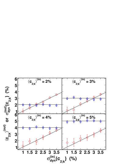
Figure 1: (color online) The reconstructed mean $v_{2}$ (stars) and its dynamical fluctuation (circles) as functions of input $\sigma_{\rm dyn}\{c_{2;k}\}$ for Monte Carlo events with multiplicity of 100. The errors are statistical. Panels are shown for input $\langle c_{2;k}\rangle$ ranging from 2% to 5%. The horizontal lines represent the input mean $v_{2}$, and the diagonal lines represent the input dynamical fluctuation of $v_{2}$.

We have also explored the robustness of the method with variations in the input values of $\langle c_{2;k}\rangle$ and $\sigma_{\rm dyn}\{c_{2;k}\}$. In this second group of tests, the multiplicity was fixed at $M=100$, and one million events were generated in each case. The reconstructed mean $v_{2}$ and the extracted dynamical fluctuations, $\sigma_{\rm dyn}\{c_{2;k}\}$, are shown in Fig. 1, and they are found to be consistent with the input values.

III Eccentricity fluctuations

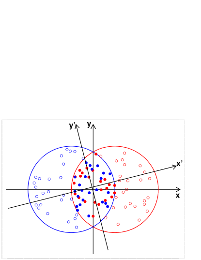
Figure 2: (color online) Schematic representation, in the plane transverse to the beam ($z$) direction, of a collision between two identical nuclei. The $x$- and $y$-axes are drawn as per the standard convention. The solid circles illustrate a possible configuration of the participant nucleons. Due to the fluctuation of this event, the overlap zone is shifted and tilted with respect to the $(x,y)$ frame. $x^{\prime}$ and $y^{\prime}$ are the principal axes of inertia of the solid circles.

In heavy-ion collisions, due to the finite number of participants, the center of the overlap zone can be shifted and the orientation of the principal axes of the interaction zone can be rotated with respect to the conventional coordinate system with the $x$ axis pointing along the impact parameter, as illustrated in Fig. 2. As a result, the final particle distribution is symmetric about the $x^{\prime}$ axis, instead of the $x$ axis. The effect of the shift is negligible compared to the effect of the rotation, and therefore we concentrate on the latter. The conclusion that the shift can be neglected is based on detailed Monte Carlo calculations using a Glauber model where the geometry of the interaction zone is defined by the position of the participating nucleons.

We define the angle between the $x^{\prime}$ and $x$ directions to be $\Delta\psi_{\varepsilon;k}$ for the $k^{\rm th}$ event.

The standard definition of eccentricity MillerSnellings for the $k^{\rm th}$ event is

$$\varepsilon_{k}=\frac{\langle y_{i}^{2}-x_{i}^{2}\rangle_{k}}{\langle y_{i}^{2}+x_{i}^{2}\rangle_{k}}$$ (19)

where $x_{i}$ and $y_{i}$ denote the $i$-th participant coordinates and the average is taken over all participants in the event. The coordinates $(x,y)$ and $(x^{\prime},y^{\prime})$ are linked by the rotation through $\Delta\psi_{\varepsilon;k}$,

$$x_{k} = x^{\prime}_{k}\cos\Delta\psi_{\varepsilon;k}-y^{\prime}_{k}\sin\Delta\psi_{\varepsilon;k}$$

$$y_{k} = x^{\prime}_{k}\sin\Delta\psi_{\varepsilon;k}+y^{\prime}_{k}\cos\Delta\psi_{\varepsilon;k}\,,$$ (20)

which leads to the relation

$$\varepsilon_{k}=\varepsilon^{\prime}_{k}\,\cos 2\Delta\psi_{\varepsilon;k}\,.$$ (21)

Note that from the definition of the rotated frame, $\langle x_{i}^{\prime}\,y_{i}^{\prime}\rangle=0$. The elliptic anisotropy in a given event is developed in the ${x^{\prime},y^{\prime}}$ plane such that $\langle s_{2;k}^{\prime}\rangle=0$ and $\sigma_{\rm dyn}\{s_{2;k}^{\prime}\}=0$. Also, similar to the relation between eccentricities, one finds

$$\langle c_{2;k}\rangle=\langle c_{2;k}^{\prime}\rangle\,\langle\cos 2\Delta\psi_{\varepsilon;k}\rangle\,,$$ (22)

which follows directly from

$$c_{2;k} = c_{2;k}^{\prime}\cos 2\Delta\psi_{\varepsilon;k}-s_{2;k}^{\prime}\sin 2\Delta\psi_{\varepsilon;k}\,,$$ (23)

$$s_{2;k} = c_{2;k}^{\prime}\sin 2\Delta\psi_{\varepsilon;k}+s_{2;k}^{\prime}\cos 2\Delta\psi_{\varepsilon;k}\,.$$ (24)

Therefore $\langle c_{2;k}\rangle$ is always less than or equal to $\langle c_{2;k}^{\prime}\rangle$.

Note that

$$c_{2;k}^{2}+s_{2;k}^{2}=c_{2;k}^{\prime\,2}+s_{2;k}^{\prime\,2}\,,$$ (25)

which reflects the fact that such a combination is independent of the plane in which it is calculated, as it depends only on the particle pair angle differences in the event. As mentioned in the previous section, this sum contains the flow fluctuation contribution (including the fluctuation in the orientation of the principal axes of the participant zone) as well as the non-flow contribution. The non-statistical part of this sum (everything except $\sim 1/M$ terms) corresponds exactly to $v_{2}^{2}\{2\}$ — elliptic flow measured with two-particle correlations at mid-rapidity. To remove non-flow contributions, one should consider the difference

$$\langle c_{2;k}^{2}-s_{2;k}^{2}\rangle=\langle c_{2;k}^{\prime\,2}-s_{2;k}^{\prime\,2}\rangle\,\langle\cos 4\Delta\psi_{\varepsilon;k}\rangle.$$ (26)

The non-statistical part of this difference,

$$\langle c_{2;k}^{2}-s_{2;k}^{2}\rangle_{\rm dyn}=\langle c_{2;k}^{\prime\,2}\rangle_{\rm dyn}\,\langle\cos 4\Delta\psi_{\varepsilon;k}\rangle,$$ (27)

provides an important relation between fluctuations measured with respect to the first-order reaction plane, $\langle c_{2;k}^{2}-s_{2;k}^{2}\rangle_{\rm dyn}$, flow fluctuations measured at mid-rapidity (which includes effects of the fluctuations in the geometry of the participant zone), and the distribution in $\Delta\psi_{\varepsilon;k}$.

In the picture described above, when the flow fluctuations are driven by fluctuations in the participant eccentricity, it is not obvious that the two first-order event planes defined by spectators from the two nuclei are independent, nor is it obvious that the first-order event plane is independent of the second-order event plane defined by the participants. Indeed, the positions of the spectators are somewhat correlated with the positions of the participants, but as we found using the Monte Carlo Glauber model, this has a negligible effect on correlations of the event planes. In our study, we used the center of gravity of the spectator distribution with respect to the nuclear center to define the first-order event plane for each nucleus ($\psi_{1,a}$ and $\psi_{1,b}$), and the second-order event plane ($\psi_{2}$) was defined by the minor axis of the participant zone. Using the center of the collision instead of the center of gravity of the spectator distribution would make the correlation effects even smaller.

We find that for most centralities, the correlations

$${{\langle\cos(\psi_{1,a}-\psi_{1,b})\rangle}\over\langle\cos(\psi_{1,a}-\Psi_{\rm RP})\rangle\,\langle\cos(\psi_{1,b}-\Psi_{\rm RP})\rangle}-1$$ (28)

and

$${\langle\cos(\psi_{1,a}+\psi_{1,b}-2\psi_{2})\rangle}\over\langle\cos(\psi_{1,a}-\Psi_{\rm RP})\rangle\,\langle\cos(\psi_{1,b}-\Psi_{\rm RP})\rangle\,\langle\cos(2\psi_{2}-2\Psi_{\rm RP})\rangle$$

$$-1~{}~{}~{}~{}~{}~{}~{}~{}~{}~{}~{}~{}$$ (29)

are at the sub-percent level, with a maximum of about a few percent for the 5% most central collisions. Besides the event plane correlations due to the correlated positions of spectators and participating nucleons, momentum conservation also deserves consideration. We refer here to an experimental study STARv1at62 which concluded that there is negligible momentum-conservation correlation between the event plane based on spectators from each nucleus separately and the orientation of directed flow close to mid-rapidity.

IV Discussion and summary

It is useful at this stage to consider the notation $\langle c_{2;k}^{\prime}\rangle\equiv\langle v_{2}^{\prime}\rangle$ and $\langle c_{2;k}^{\prime\,2}\rangle_{\rm dyn}=\langle v_{2}^{\prime\,2}\rangle$  , where $v_{2}^{\prime}$ is the “apparent” flow at mid-rapidity — elliptic event anisotropy measured with respect to the principal axes of the participant zone. Much progress towards a direct measurement of flow fluctuations at mid-rapidity has been reported recently Phobos06 ; SorensenQM06 . Then the above equations can provide important information on fluctuations in the orientation of the principal axes of the participant zone.

Note that the orientation of the participant zone (and, consequently, the apparent anisotropic flow) can depend on the rapidity of the particles under study. Then, in principle, one can study the correlations in the orientation of anisotropic flow as function of particle rapidity. Such information will be very valuable for the reconstruction of the initial conditions in heavy-ion collisions.

In summary, various suggestions in the literature point to dynamical event-by-event fluctuations in elliptic flow as being of great interest in the realm of RHIC physics, and such fluctuations are argued to be especially relevant for understanding collision dynamics at the earliest times. On a more technical level in experimental methodology, the magnitude of flow fluctuations associated with current elliptic flow measurements is not understood, and this uncertainty affects the overall systematic error on these measurements. Prompted by the above considerations, this work presents a new method for experimental analysis of elliptic flow in a scenario where the first-order event plane can be resolved. The method allows the extraction of mean $v_{2}$ and its dynamical event-by-event fluctuations, and good immunity to both statistical fluctuations and non-flow effects can be expected. Simulations have been presented that validate the method under a range of conditions similar to those observed in RHIC data. It has been shown that measurements of flow fluctuations using the first-order event plane, accompanied by measurements of apparent flow fluctuations at mid-rapidity, can also provide important information on the fluctuations of the participant zone.

- (1) S. Voloshin and Y. Zhang, Z. Phys. C 70, 665 (1996); A. M. Poskanzer and S. A. Voloshin, Phys. Rev. C58, 1671 (1998).
- (2) STAR Collaboration, C. Adler et al., Phys. Rev. C66, 034904 (2002).
- (3) STAR Collaboration, J. Adams et al., Phys. Rev. C72, 014904 (2005).
- (4) M. Miller and R. Snellings, preprint nucl-ex/0312008
- (5) S. Mrówczyński and E. Shuryak, Acta Phys. Polon. B 34, 4241 (2003).
- (6) PHOBOS collaboration, B. Alver et al., preprints nucl-ex/0608025 and nucl-ex/0702036
- (7) STAR Collaboration, P. Sorensen et al., preprint nucl-ex/0612021
- (8) S. Mrówczyński, Phys. Lett. B 314, 118 (1993); Phys. Rev. C49, 2191 (1994); Phys. Lett. B 393, 26 (1997).
- (9) Y. V. Kovchegov and K. L. Tuchin, Nucl. Phys. A 708, 413 (2002).
- (10) A. Krasnitz, Y. Nara and R. Venugopalan, Phys. Lett. B 554, 21 (2003).
- (11) E. Shuryak, Nucl. Phys. A 715, 289 (2003).
- (12) C. Adler et al., Nucl. Instr. Meth. A470, 488 (2001); The STAR ZDC-SMD has the same structure as the STAR EEMC SMD: C. E. Allgower et al., Nucl. Instr. Meth. A499, 740 (2003); STAR ZDC-SMD proposal, STAR Note SN-0448 (2003).
- (13) K. H. Ackermann et al., Nucl. Instr. Meth. A 499, 713 (2003).
- (14) STAR Collaboration, J. Adams et al., Phys. Rev. C73, 034903 (2006).