Moment Analysis and Zipf Law

Abstract

The moment analysis method and nuclear Zipf’s law of fragment size distributions are reviewed to study nuclear disassembly. In this report, we present a compilation of both theoretical and experimental studies on moment analysis and Zipf law performed so far. The relationship of both methods to a possible critical behavior or phase transition of nuclear disassembly is discussed. In addition, scaled factorial moments and intermittency are reviewed.

1 Introduction

Hot nuclei can be formed in energetic heavy ion collisions (HIC) and deexcite by different decay modes, such as evaporation and multifragmentation. Experimentally, multifragment emission was observed to evolve with excitation energy. The multiplicity, $N_{imf}$, of intermediate mass fragment (IMF) rises with the beam energy, reaches a maximum, and finally falls to a lower value. The onset of multifragmentation may indicate the coexistence of liquid and gas phases Maprc95 . Phenomenologically, the mass (charge) distribution of IMF distribution can be expressed as a power law with parameter $\tau_{eff}$, and a minimum $\tau_{min}$ of $\tau_{eff}$ emerges around the onset point, which suggests that a kind of critical behavior may take place. In the framework of Fisher’s droplet model, the mass distribution can be described by a power law with a critical exponent of $\tau\sim 2.3$ when the system is in the vicinity of the critical point Fisher .

On the other hand, the caloric curve measurement can also provide useful information on the liquid-gas phase transition Albergo ; Poch ; Ma-PLB97 ; JBN0 ; JBN1 . The analysis of other independent critical exponents provides additional indications of critical behavior of finite nuclear systems Bau0 ; Gilk ; Ago ; Ell1 ; Ell2 ; Bau1 . In addition, more observables have been proposed to sign the liquid-gas phase transition or critical behavior of nuclei Ma2005 ; Richert_PhysRep ; Dasgupta_01 ; Bonasera ; Chomaz_INPC ; Moretto_INPC . Some reviews can be found in this volume JBN-WCI ; Viola-WCI ; Borderie-WCI ; Gul-WCI ; Lopez-WCI .

In this report, we shall review the moment analysis method and Zipf law of fragment size distribution. The phenomenological basis of moment analysis is introduced in Sec. 2. Finite size effects are discussed in Sec.3. Section 4 gives the application of moment analysis to multifragmention and its relation to critical behavior. Scaled factorial moments and intermittency are discussed in Sec. 5. In Sec. 6 Zipf law is introduced for the nuclear fragment distribution and the corresponding simulations are given; some experimental indications of nuclear Zipf law are presented in Sec. 7; finally the summary and outlook are given in Sec. 8.

2 Phenomenological Basis of Moment Analysis

Campi Campi-JPA86 ; Campi-PLB88 and Bauer Bauer-PLB85 ; Bauer-NPA86 et al. first suggested that the methods used in percolation studies may be applied to nuclear multifragmentation data. In percolation theory the moments of the cluster distribution contain a signature of critical behavior Stauffer . The method of moment analysis has been experimentally used to search for evidence of the critical behavior in multifragmentation. The definition of the $k$ moments of the cluster size distribution for each event is

$$M_{k}=\sum_{A\neq A_{max}}A^{k}n_{A},$$ (1)

where $A$ is the fragment mass, and $n_{A}$ is the number of charged fragments whose charge is $Z$ and mass is $A$. The sum runs over all masses $A$ in the event including neutrons except the heaviest fragment ($A_{max}$). This quantity was taken as a basic tool in extracting critical exponents in Au + C data Gilk . It has been argued that there should be an enhancement in the critical region of the moment $M_{k}$, for $k>\tau-1$, with a critical exponent $\tau>2$ Campi-JPA86 ; Campi-PLB88 .

In experimental analyses, events are sorted by different conditions. In this case, so-called conditional moments are used to describe the fragment distribution. Usually the mean value of $M_{k}(m)$ for events with given control parameters, e.g. the moment $M_{k}$ for events with a given multiplicity $m$, or total bound charge number $Z_{bound}$, or excitation energy $E^{*}$, is called conditional moment.

More insight in the shape of the fragment size distribution is obtained by looking at a combination of moments $M_{k}$. For example, the quantity

$$\gamma_{2}=\frac{M_{2}M_{0}}{M_{1}^{2}}=\frac{\sigma^{2}}{\langle s\rangle^{2}}+1,$$ (2)

has been used, where $M_{1}$ and $M_{2}$ are the first and second moments of the mass distribution and $M_{0}$ is the total multiplicity including neutrons. $\sigma^{2}$ is the variance of the fragment distribution and $\langle s\rangle=M_{1}/M_{0}$ represents the mean fragment size. $\gamma_{2}$ takes the value $\gamma_{2}=2$ for a pure exponential distribution $N(s)\sim exp(-\alpha s)$ regardless of the value of $\alpha$, but $\gamma_{2}\gg 2$ for a power-law distribution $N(s)\sim s^{-\tau}$ when $\tau>2$. In the percolation model, the position of the maximum $\gamma_{2}$ value defines the critical point, where the fluctuations in the fragment size distribution are the largest. In principle a genuine critical behavior requires the peak value of $\gamma_{2}$ to be larger than 2 Campi-JPA86 ; Campi-PLB88 . However, due to finite size effects, this is not always true when the system size decreases, as we will see in the following sections.

Campi also suggested to use the single event (j) moment, i.e.

$$M_{k}^{(j)}=\sum_{A\neq A_{max}}A^{k}n^{(j)}$$ (3)

to investigate the shape of fragment size distribution. Also normalized moments Campi-JPA86

$$S_{k}^{(j)}={M_{k}^{(j)}}/{M_{1}^{(j)}}$$ (4)

can be defined. It was suggested to use the event-by-event scatter-plots of the natural log of the size ($A_{max}$) or charge number ($Z_{max}$) of the largest cluster, ln$A_{max}$ or ln$Z_{max}$ versus the natural log of the second moment, ln$M_{2}$, or the normalized moment ln$S_{2}$ to search for the largest fluctuation point. Some examples will be given in the following sections.

In the percolation model, the cluster size distribution for infinite systems near a critical point can be expressed by

$$n(s)\sim s^{-\tau}f(\epsilon s^{\sigma}).$$ (5)

where $s$ is the size of finite clusters, $\tau$ and $\sigma$ two critical exponents and $\epsilon$ a variable that characterizes the state of the system. In thermal phase transitions $\epsilon=T-T_{c}$ is the distance to the critical temperature $T_{c}$. In percolation $\epsilon=p_{c}-p$ is the distance to the critical fraction of active bonds or occupied sites $p_{c}$. The scaling function $f(\epsilon s^{\sigma})$ satisfies $f(0)$ = 1, decaying rapidly (exponentially) for large values of $|\epsilon|$. In addition, theory predicts that when $\epsilon<0$ one infinite cluster (liquid or gel) is present in the system while no such cluster exists when $\epsilon>0$ (only droplets or $n$-mers). In finite systems a similar behavior is observed, especially when the largest cluster is counted separately.

The moment analysis method is useful to obtain some information about the possible occurrence of a critical behavior. In general, critical exponents can be defined according to the standard procedure followed in condensed matter physics Binder . For example,

$$M_{k}(\epsilon)=\sum_{A}=A^{k}n_{A}(\epsilon)\sim|\epsilon|^{\frac{\tau-k-1}{\sigma}},(\epsilon\to 0)$$ (6)

where $\tau$ and $\sigma$ are the critical exponents. For the percolation phase transition and the critical point in the Fisher droplet model, the exponent $\tau$ satisfies $2<\tau<3$ and thus the second and high moments diverge at the critical point. In contrast the lower moments $M_{0}$ and $M_{1}$, which correspond to the number of fragments and the total mass, do not diverge.

Based upon the scaling relation Eq. (5), there exists the following relationship between critical exponents and moments:

$$M_{0}\sim|\epsilon|^{2-\alpha},$$

$$M_{1}\sim|\epsilon|^{\beta},$$

$$M_{2}\sim|\epsilon|^{-\gamma},$$ (7)

where $\beta$ and $\gamma$ are two other critical exponents. Some relationships among critical exponents exist (hyperscaling relations), for instance

$$2\beta+\gamma=\frac{\tau-1}{\sigma}=2-\alpha.$$ (8)

In finite systems transitions are smooth, but it is still possible to determine some critical exponents, as we will discuss in the next section. By analogy with the infinite system behavior, one says that these moments exhibit a critical behavior also for finite systems. In particular in the Fisher model, the thermal critical point is also a critical point for moments of the fragment size distribution.

In order to illustrate the application of moment analysis, we show the EOS data and NIMROD data as examples in Sec. 4.

3 Finite Size Effects

Since the nucleus is a finite size system, the macroscopic thermal limit cannot be applied. Therefore finite size effects on phase transition behavior should be checked. In this section, we give some examples to illustrate this problem.

A percolation on a cubic lattice of linear size $L$ containing $L^{3}$ sites, for $L$ = 4 to 10, where all sites are occupied and bonds are assumed to exist between neighbouring sites with bond probability $p$, has been considered Jaqaman . Sites that are connected together by such bonds are said to belong to the same cluster. It is well known that in such a model there exists a critical (or threshold) probability $p_{c}$ such that for $p>p_{c}$ there is a large cluster that percolates throughout the lattice from end to end whereas for $p<p_{c}$ no such cluster exists and all the sites belong to small clusters (including isolated sites, i.e. singlet or clusters of size 1). As $L\to\infty$ the transition becomes sharper and $p_{c}$ approaches a limiting value which for bond percolation on a cubic lattice is $p_{c}$ = 0.249 Stauffer . For finite systems the threshold percolation probability is not so sharply defined.

In order to quantitatively illustrate finite size effects on critical behavior, the average of normalized second moment $S_{2}$ ($\overline{S_{2}}$) over all events belonging to the same value of ln($A_{max}$) was calculated Jaqaman . The results obtained by such averaging are presented by the dots shown in Fig. 1 for various cubic lattices with linear dimension $L$ = 4 - 10 sites Jaqaman . The location of the maximum value of $\overline{S_{2}}$ is now defined as corresponding to the location of the critical point, which is a standard way of determining the percolation threshold Jan . The slope of the lower branches of the curves in Fig. 1 can also be calculated. This slope is expected to be 1 + $\beta/\gamma$ which for percolation in three dimensions is equal to 1.23. For comparison the slopes of the straight lines by a lest-squares fit to the lower branches of the $L$ = 4 to 10 curves are found, in ascending order of $L$, to have the values 1.582$\pm$0.036, 1.503$\pm$0.029, 1.375$\pm$0.017, 1.355$\pm$0.021, 1.260$\pm$0.007, 1.258$\pm$0.014 and 1.242$\pm$0.015 Jaqaman . This indicates that these slopes rapidly approach the value expected in the thermodynamic limit. In calculating these slopes one has excluded the points near the bottom of the branch in the region where the curves in Fig. 1 deviate noticeably from a straight line. These points correspond to events that are far from the critical region.

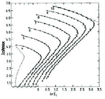
Figure 1: The logarithm of the largest fragment size $A_{max}$ as a function of the logarithm of the corresponding average normalized second moment $\overline{S_{2}}$ for bond percolation on simple cubic lattices of linear size ranging from $L$ = 4 - 10 sites. The dots represent the actual calculation results and the curves drawn are just to guide the eye. The number next to each curve gives the value of the linear size $L$. Note that the ln$\overline{S_{2}}$ scale given corresponds to the $L$ = 10 curve. The other curves are successively shifted to the left with respect to each other by a distance of 0.25. The dashed curve and the dotted-dashed straight line are explained in the text. Figure is taken from Ref. Jaqaman .

Similarly to the analysis for the correlation of $\overline{S_{2}}$ and ln($A_{max}$), finite size effects have been also investigated for $M_{2}$ by Campi Campi-PLB88 . This is shown in Fig. 2, where $M_{2}(n)$ is plotted for various system sizes ($50^{3},9^{3},5^{3}$ and $3^{3}$) in a percolation model. We see clearly the critical behavior for the largest system, namely a well defined peak, and how this peak is smoothed when decreasing the size Campi-PLB88 .

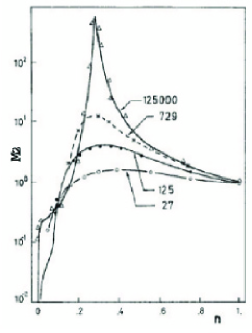
Figure 2: The conditional moments $M_{2}(n)$ for percolation in a cubic lattice of linear size $L$ = 3, 5, 9 and 50 (the corresponding cubic lattice is $L^{3}$ which is shown as the number in the insert). The figure is taken from Ref. Campi-PLB88 .

4 Application of the Moment analysis method

4.1 EOS data

4.1.1 Experimental description

The reverse kinematic EOS experiment was performed with 1 A GeV ¹⁹⁷Au, ¹³⁹La, and ⁸⁴Kr beams on carbon targets. The experiment was done with the EOS Time Project Chamber (TPC) and multiple sampling ionization chamber (MUSIC II). The excellent charge resolution of this detector permitted identification of all detected fragments. The fully reconstructed multifragmentation events for which the total charge of the system was taken as $79\leq Z\leq 83$, $54\leq Z\leq 60$, $33\leq Z\leq 39$ for Au, La, and Kr, respectively SrivastavaPRC65 ; Scharenberg ; HaugerPRC57 ; HaugerPRC62 were analyzed. The remnant refers to the equilibrated nucleus formed after the emission of prompt particles. The charge and mass of the remnant were obtained by removing for each event the total charge of the prompt particles. The excitation energy of the remnant $E^{*}$ was based on an energy balance between the excited remnant and the final stage of the fragments for each event Cussol . The thermal excitation energy $E_{th}^{*}$ of the remnant was obtained as the difference between $E^{*}$ and $E_{x}$ which is a nonthermal component, namely an expansion energy SrivastavaPRC65 ; Scharenberg ; HaugerPRC57 ; HaugerPRC62 ; LauretPRC57 .

4.1.2 Determination of Critical Point and Exponent in Terms of Moment Analysis

The determination of the critical point and the associated exponents in the multifragmentation of gold nuclei was first attempted by the EOS collaboration Gilk . In their early publication Gilk , they use the multiplicity $m$, as a control variable for the collision violence and assume that $m$ is a linear measure of the distance from the critical point. Then the critical exponents $\beta$, $\gamma$ and $\tau$, can be determined according to Eqs. (7,8) above. They find that these exponents are close to the nominal liquid-gas universality class values. However, this method is very delicate. In particular, due to the small size of the system, an important rounding of the transition is expected which may distort considerably the determined critical exponents. For a review of this debate, see the arguments between Bauer Bauer2 and Gilkes Gilk2 .

A different analysis was also proposed by the EOS collaboration Elliott_PRC03 . In this work, thermal excitation energy has been taken as a control variable, which is believed to be more suitable to characterize the collision violence.

The $\gamma_{2}$ analysis is shown in Fig. 3 for all three systems. The position of the maximum $\gamma_{2}$ value defines the critical excitation energy $E^{*}_{c}$, which corresponds to the largest fluctuation point in the fragment size distribution. The peak in $\gamma_{2}$ is well defined for La and Au. For Kr, the peak is very broad and the value $\gamma_{2}$ is less than 2.

Fig. 3 also shows a $\gamma_{2}$ calculation using the statistical multifragmentation model (SMM). The fission contribution to $\gamma_{2}$ has been removed both from the data and SMM. In the case of Au, the $\gamma_{2}$ value remains above two for most of the excitation energy range both in data and SMM. The $E_{th}^{*}$ width over which $\gamma_{2}>2$ is smaller for La and disappears for Kr. The decrease in $\gamma_{2}$ with decreasing system size is also seen in 3D percolation studies and these differences have been attributed to finite size effects Elliott_PRC03 ; Campi92a ; Campi92b .

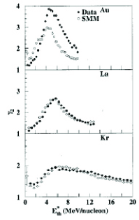
Figure 3: $\gamma_{2}$ as a function of $E_{th}^{*}$ for all three systems of 1 A GeV Au, La, and Kr collisions with C target and SMM calculations. Figure is taken from Ref. SrivastavaPRC65 .

The exponent $\tau$ can be obtained if the second moment $M_{2}$ and the third moment $M_{3}$ of the fragment mass distributions are known. A plot of ln($M_{3}$) vs ln($M_{2}$) should give a straight line with a slope given by

$$S=\frac{\Delta ln(M_{3})}{\Delta ln(M_{2})}=\frac{\tau-4}{\tau-3}.$$ (9)

Fig. 4 shows a scatter-plot of ln($M_{3}$) vs ln($M_{2}$) for the three systems constructed with data above the critical excitation energy $E_{c}^{*}$ (see Fig. 3) and with SMM simulations. A linear fit to ln($M_{3}$) vs ln($M_{2}$) gives the value of $\tau$. The fitted $\tau$ values are $2.16\pm 0.08$, $2.10\pm 0.06$ and $1.88\pm 0.08$, respectively. The former two are very close to the critical exponents $\tau\sim 2.3$ of the liquid-gas universal class.

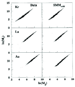
Figure 4: ln($M_{3}$) vs ln($M_{2}$) for Au, La, and Kr above the critical energy. Figure is taken from Ref. SrivastavaPRC65 .

The exponent $\beta$ can be obtained for the multifragmentation data by the relation

$$A_{max}\sim|\epsilon|^{\beta},$$ (10)

where $\epsilon=p-p_{c}$ and $\epsilon>0$. In the multifragmentation case of this work $p$ and $p_{c}$ have been replaced by $E^{*}_{th}$ and $E_{c}^{*}$. In an infinite system, the finite cluster exists only on the liquid side of $p_{c}$. In a finite system a largest cluster is present on both sides of the critical point, but the above equation holds only on the liquid side. Fig. 5 shows a plot of ln$(A_{max})$ vs ln$|E^{*}_{th}-E_{c}^{*}|$ for Au, La, and Kr. The values of $\beta$ extracted for Au and La are 0.32$\pm$0.02 and 0.34$\pm$0.02, respectively, which are close to the value of 0.33 predicted for a liquid-gas phase transition. On the other hand, the value of $\beta$ = 0.53 $\pm$ 0.05 for Kr is much higher than that of Au and La.

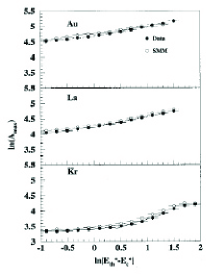
Figure 5: ln($A_{max}$) vs ln$|E^{*}_{th}-E_{C}^{*}|$ for Au, La, and Kr below the critical energy for exponent $\beta$ determination. Figure is taken from Ref. SrivastavaPRC65 .

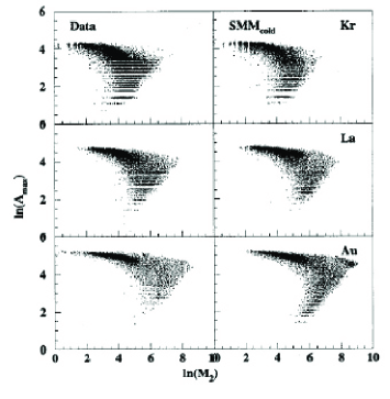
Figure 6: Scatter-plots of ln($A_{max}$) vs ln($M_{2}$) from the data for Au, La, and Kr. Left panel: EOS data; Right panel: SMM simulation. The figure is taken from Ref. SrivastavaPRC65 .

As shown in Sec. 2, Campi also suggested that the correlation between the size of the biggest fragment $A_{max}$ and the moments in each event, i.e. the scatter-plot, can measure the critical behavior in nuclei. Fig. 6 depicts a scatter- plot with logarithmic scale for Au, La, and Kr of EOS data. The two branches corresponding to the sub-critical (upper branch) and overcritical (lower branch) events are clearly seen for Au and La. The scatter-plot is very broad for Kr and fills most of the available space. The sub- and over-critical branches seem to overlap and are not well separated. Studies on SMM show a similar behavior. If one knows the location of the critical point from some other methods, then the scatter-plot can be used to calculate the ratio of critical exponents $\beta/\gamma$ from the slope of the sub-critical branch. In EOS data, the position of the largest $\gamma_{2}$ was used to define the critical point, which corresponds to the largest fluctuation of the fragment distribution. In this context, $\beta/\gamma$ values for Au, La and Kr can be extracted from the linear fit to the upper branch; they are 0.22 $\pm$ 0.03, 0.25 $\pm$ 0.01 and 0.50 $\pm$ 0.01, respectively. $\beta/\gamma$ values of Au and La are close to the value 0.26 expected for the liquid-gas universality class.

To summarize the critical exponent analysis of the EOS data, the experimental results in conjunction with SMM provide some indications on the order of the phase transition in Au, La and Kr. The values of the critical exponents $\tau$, $\beta$, and $\gamma$, which are close to the values of a liquid-gas system, along with nearly zero latent heat (this subject is beyond the discussion topics in this review, but the interested reader is reported to Refs. SrivastavaPRC65 ; Scharenberg ) have been interpreted by the authors as a continuous phase transition in Au and La. However, the analysis of Kr leads to very different critical exponents. A recent analysis based on the shape of SMM microcanonical caloric curve indicates a first order phase transition for the multifragmentation of Kr SrivastavaPRC65 ; Scharenberg .

4.2 NIMROD data

4.2.1 Experimental set-up and Analysis Details

Using the TAMU NIMROD (Neutron Ion Multidetector for Reaction Oriented Dynamics) and beams from the TAMU K500 super-conducting cyclotron, we have probed the properties of excited projectile-like fragments produced in the reactions of 47 MeV/nucleon ⁴⁰Ar + ²⁷Al, ⁴⁸Ti and ⁵⁸Ni. The charged particle detector array of NIMROD, which is set inside a neutron ball, includes 166 individual CsI detectors arranged in 12 rings in polar angles from $\sim$ $3^{\circ}$ to $\sim$ $170^{\circ}$. The detailed description for the experiment can be found in Ma2005 . The correlation of the charged particle multiplicity ($M_{cp}$) and the neutron multiplicity ($M_{n}$) was used to sort the event violence. After the reconstruction of the quasi-projectile (QP) particle source, the excitation energy was deduced event-by-event using the energy balance equation Cussol .

4.2.2 Critical Point Determination via Moment Analysis

In Fig. 7 we present Campi scatter-plots for the nine selected excitation energy bins. In the low excitation energy bins of $E^{*}/A$ $\leq$ 3.7 MeV/u, the upper (liquid phase) branch is strongly dominant while at $E^{*}/A$ $\geq$ 7.5 MeV/u, the lower $Z_{max}$ (gas phase) branch is strongly dominant. In the region of intermediate $E^{*}/A$ of 4.6- 6.5 MeV/u, the transition from the liquid dominated branch to the vapor branch occurs, indicating that the region of maximal fluctuations is to be found in that range.

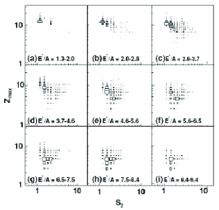
Figure 7: Campi plots for nine intervals of excitation energy for the QP formed in ⁴⁰Ar + ⁵⁸Ni. Figure is taken from Ref. Ma2005 .

The excitation energy dependence of the average values of $\gamma_{2}$ obtained in an event-by-event analysis of our data are shown in Fig. 8. $\gamma_{2}$ reaches its maximum in the 5-6 MeV excitation energy range. In contrast to observations for heavier systems of Au and La SrivastavaPRC65 ; Elliott_PRC03 , there is no well defined peak in $\gamma_{2}$ for our very light system and $\gamma_{2}$ is relatively constant at higher excitation energies. This is similar to the case of Kr of EOS data. We note also that the peak value of $\gamma_{2}$ is lower than 2 which is the expected smallest value for critical behavior in large systems. However, 3D percolation studies indicate that finite size effects can lead to a decrease of $\gamma_{2}$ with system size Campi92a ; Campi92b . For a percolation system with 64 sites, peaks in $\gamma_{2}$ under two are observed. Therefore, the criterion $\gamma_{2}>2$ alone is not sufficient to discriminate whether or not the critical point is reached.

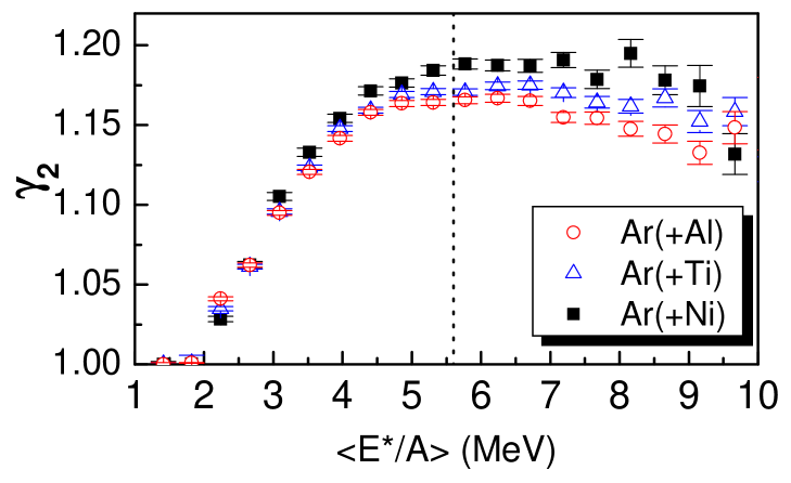
Figure 8: $\gamma_{2}$ of the QP systems formed in Ar + Al (open circles), Ti (open triangles) and Ni (solid squares) as a function of excitation energy.

In the Fisher droplet model, the critical exponent $\tau$ can be deduced from the cluster distribution near the critical point. To quantitatively pin down the possible phase transition point, we use a power law fit to the QP charge distribution in the range of $Z$ = 2 - 7 (Fig. 9) to extract the effective Fisher-law parameter $\tau_{eff}$ by

$$dN/dZ\sim Z^{-\tau_{eff}}.$$ (11)

Fig. 10(a) shows the effective Fisher-law parameter $\tau_{eff}$ as a function of excitation energy. A minimum with $\tau_{eff}$ $\sim$ 2.3 is seen to occur in the $E^{*}/A$ range of 5 to 6 MeV/u Ma_NPA2005 . This value is close to the critical exponent of the liquid-gas phase transition universality class Fisher .

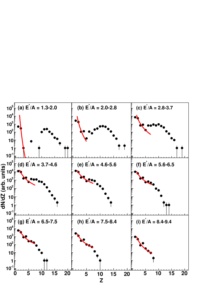
Figure 9: Charge distribution of QP in different $E^{*}/A$ window for the reaction ⁴⁰Ar + ⁵⁸Ni. Lines represent fits. Figure is taken from Ref. Ma2005 .

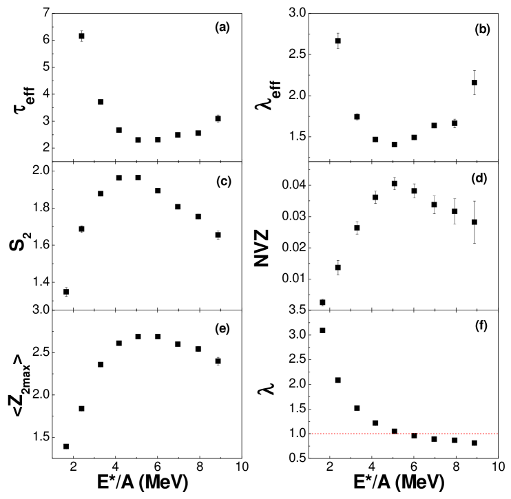
Figure 10: The effective Fisher-law parameter ($\tau_{eff}$) (a), the effective exponential law parameter ($\lambda_{eff}$) (b), $\langle S_{2}\rangle$ (c), NVZ fluctuation (d), the mean charge number of the second largest fragment $\langle Z_{2max}\rangle$ (e), the Zipf-law parameter $\lambda$ (f). See details in text. Figure is taken from Ref. Ma_NPA2005 .

Assuming that the heaviest cluster in each event represents the liquid phase, we have attempted to isolate the gas phase by event-by-event removal of the heaviest cluster from the charge distributions. We find that the resultant distributions are better described with an exponential form $exp^{-\lambda_{eff}Z}$. The fitting parameter $\lambda_{eff}$ was derived and is plotted against excitation energy in Fig. 10(b). A minimum is seen in the same region where $\tau_{eff}$ shows a minimum. To further explore this region we have investigated other proposed observables commonly related to fluctuations and critical behavior. Fig. 10(c) shows the mean normalized second moment, $\langle S_{2}\rangle$ as a function of excitation energy. A peak is seen around 5.6 MeV/u, it indicates that the fluctuation of the fragment distribution is the largest in this excitation energy region. Similarly, the normalized variance in $Z_{max}/Z_{QP}$ distribution (i.e. NVZ = $\frac{\sigma^{2}_{Z_{max}/Z_{QP}}}{\langle Z_{max}/Z_{QP}\rangle}$) Dorso shows a maximum in the same excitation energy region (Fig. 10(d)), which illustrates the maximal fluctuation for the largest fragment is reached around $E^{*}/A$ = 5.6 MeV. The second largest fragment shows a behavior similar to the one of the largest fragment. Fig. 10(e) shows a broad peak of $\langle Z_{2max}\rangle$ - the average atomic number of the second largest fragment - also occurring in the same excitation energy range around 5.6 MeV/u.

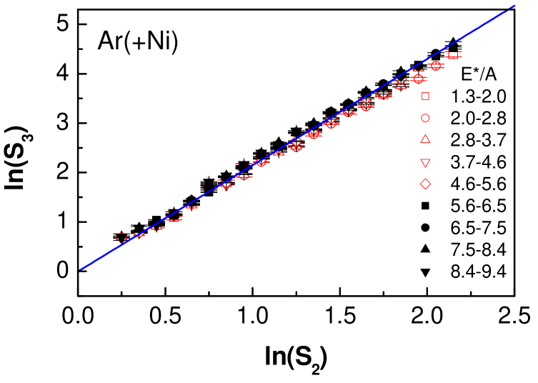
Figure 11: The correlation between ln($S_{3}$) vs ln($S_{2}$) and a linear fit.

More variables have been collected to support the determination of the critical point around 5.6 MeV/u of excitation energy for our system Ma2005 , such as $\Delta$-scaling Botet or energy fluctuations Gul-WCI . In addition, the measurement of the caloric curve Ma2005 gives a temperature, $T_{c}\sim$ 8.3 MeV around $E^{*}/A$ = 5.6 MeV. The value of the critical temperature is needed for the determination of the critical exponents, as explained in the following subsection.

4.2.3 Determination of Critical Exponents Based on Moment Analysis

In terms of the scaling theory, $\tau$ can also be deduced from Eq. (9). Since the value of $T_{c}$ = 8.3 MeV has been determined from our caloric curve measurements Ma2005 , we can explore the correlation of $S_{2}$ and $S_{3}$ in two ranges of excitation energy (see Figure 11). The moments were calculated by excluding the species with $Z_{max}$ for the ”liquid” phase but including it in the ”vapor” phase. The slopes were determined from linear fits to the ”vapor” and ”liquid” regions respectively and then averaged. In this way, we obtained a value of $\tau=2.13\pm 0.1$.

Other critical exponents can also be related to other moments of the cluster distribution, $M_{k}$. Using our caloric curve measurements Ma2005 , we can use temperature as a control parameter for such determinations. Then the critical exponent $\beta$ can be extracted from the relation

$$Z_{max}\propto(1-\frac{T}{T_{c}})^{\beta},$$ (12)

and the critical exponent $\gamma$ can be extracted from the second moment via

$$M_{2}\propto|1-\frac{T}{T_{c}}|^{-\gamma}.$$ (13)

In both equations, $|1-\frac{T}{T_{c}}|$ is the parameter which measures the distance from the critical point.

The upper panel of Fig. 12 explores the dependence of $Z_{max}$ on $(1-\frac{T}{T_{c}})$. A dramatic change of $Z_{max}$ around the critical temperature $T_{c}$ is observed. Lattice-gas model (LGM) calculations also predict that the slope of $Z_{max}$ vs $T$ will change at the liquid-gas phase transition Ma_JPG01 . Using the liquid side points, we can deduce the critical exponent $\beta$ by $ln(Z_{max})$ vs $ln|1-T/T_{c}|$. Fig. 12(a) shows the extraction of $\beta$ using Eq. (12). An excellent fit was obtained in the region away from the critical point, which indicates a critical exponent $\beta$ = 0.33 $\pm$ 0.01. Near the critical point, finite size effects become stronger so that the scaling law is violated. The extracted value of $\beta$ is that expected for a liquid-gas transition (See Table 1) Stauffer .

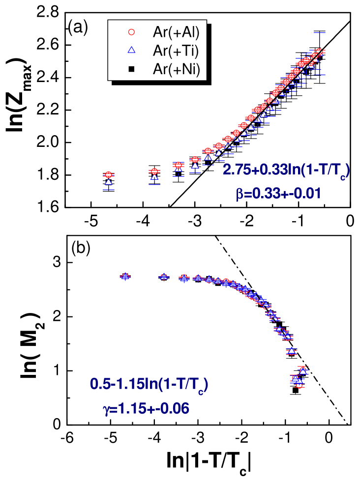
Figure 12: The extraction of the critical exponent $\beta$ (a) and $\gamma$ (b). See texts for details.

To extract the critical exponent $\gamma$, we take $M_{2}$ on the liquid side without $Z_{max}$. Fig. 12(b) shows ln($M_{2}$) as a function of ln($|1-\frac{T}{T_{c}}|$). We center our fit to Eq. (13) about the center of the range of $(1-T/T_{c})$ which leads to the linear fit and extraction of $\beta$ as represented in Figure 12. We obtain a critical exponent $\gamma$ = 1.15 $\pm$ 0.06. This value of $\gamma$ is also close to the value expected for the liquid-gas universality class (see Table 1). It is seen that the selected region has a good power law dependence.

Since we have the critical exponent $\beta$ and $\gamma$, we can use the scaling relation

$$\sigma=\frac{1}{\beta+\gamma},$$ (14)

to derive the critical exponent $\sigma$. In such way, we get the $\sigma$ = 0.68 $\pm$ 0.04, which is also very close to the expected critical exponent of a liquid-gas system.

To summarize the critical exponents extracted from NIMROD data, we present the results in Table 1 as well as the values expected for the 3D percolation and liquid-gas universality classes. It is apparent that our values for this light system with A$\sim$36 are closer to the values of the liquid-gas phase transition universality class rather than to the 3D percolation class.

Table 1: Comparison of the Critical Exponents

Exponents	3D Percolation	Liquid-Gas	NIMROD
$\tau$	2.18	2.21	2.13$\pm$0.10
$\beta$	0.41	0.33	0.33$\pm$0.01
$\gamma$	1.8	1.23	1.15$\pm$0.06
$\sigma$	0.45	0.64	0.68$\pm$0.04

5 Scaled factorial moments and intermittency

Intermittency is related to the existence of large non-statistical fluctuations and is a signal of self-similarity of the fluctuation distribution at all scales. This signal can be deduced from the scaled factorial moments Bialas ,

$$F_{k}(\delta)=\frac{\Sigma_{i=1}^{X_{max}/\delta}\langle n_{i}(n_{i}-1)(n_{i}-2)...(n_{i}-k+1)\rangle}{\Sigma_{i=1}^{X_{max}/\delta}\langle n_{i}\rangle^{k}}$$ (15)

where $X_{max}$ is an upper characteristic value of the system (i.e. total mass or charge, maximum transverse energy or momentum, etc.) and $k$ is the order of the moment. The total interval 0-$X_{max}$ (1-$A_{max}$, $Z_{max}$ in the case of mass or charge distributions) is divided into $X_{max}/\delta$ bins of the size $\delta$, $n_{i}$ is the number of particles in the $i$th bin for an event, and the ensemble average $\langle\rangle$ is performed over all events. The concept of intermittency was originally developed in the field of fluid dynamics to study the fluctuations occurring in turbulent flows Mandelbrot ; Zeldovich . Its presence in the velocity and temperature distributions is established by the existence of large non-statistical fluctuations which exhibit scale invariance. Intermittency in physical systems is studied by examining the scaling properties of the moments of the distributions of relevant variables over a range of scales Paladin . The concept of intermittency was first introduced for the study of dynamical fluctuations in the density distribution of particles produced in high energy collisions by Bialas and Peschanski Bialas . It soon led to the discovery of a characteristic power law dependence of the factorial moments, $F_{k}$, of an order $k$ on the resolution scale, $\delta$: $F_{k}\propto(1/\delta)^{f(k)}$. The specific properties of the intermittency exponent, $f(k)$, can be associated either with a random production process Bialas ; Bialas2 or with a second-order phase transition Bialas2 ; Hwa-int ; Feynman depending on the values obtained. Thus an analysis of the factorial moments may provide important information on the dynamical properties of the system. Ploszajczak and Tucholski were the first to suggest searching for intermittency patterns in the mass and charge distributions of the fragments produced in energetic collisions Plo1 . Since then many studies show that an intermittency pattern of fluctuations in the fragmentation charge distributions has been observed in many data and models. Much effort has been devoted to find the relation between fragmentation, a possible critical behavior, and intermittency Dorso ; Phair ; Elattari ; Barz ; Latora ; Campi .

Intermittency is defined by the relation

$$F_{k}(\delta^{\prime})\equiv F_{k}(a\delta)=a^{-f(k)}F_{k}(\delta),$$ (16)

between factorial moments $F_{k}(\delta^{\prime})$ and $F_{k}(\delta_{s})$ obtained for two different binning parameters $\delta$ and $\delta^{\prime}$ = a$\delta$. Intermittency implies a linear relationship in the double logarithmic plot of $lnF_{k}$ versus $-ln\delta$.

The fractal intermittency exponent, $f(k)$, is related to the factorial dimension $d_{k}$ by

$$f(k)=\frac{d_{k}}{k-1}>0.$$ (17)

Different processes seem to give a different behavior of these anomalous fractal dimension $d_{k}$: (1) $d_{k}$ = constant corresponds to a monofractal, second order phase transition in the Ising model and in the Feynman-Wilson fluid Hwa-int ; Feynman . It has been also demonstrated that in the case of a second order phase transition in the Ginzburg-Landau description one gets $d_{k}=d_{2}(k-1)^{\mu-1}$ with $\mu=1.304$ Hwa-int . (2) $d_{k}\propto k$ correspond to multifractal, cascading processes Bialas . Therefore, a study of the anomalous fractal dimensions can give useful information about the evolution of the system.

Several models have been introduced to study the intermittency signal. One of the simplest models, widely used in the analysis of experimental data and which gives intermittency, is the percolation model. Percolation models predict a phase transition corrected for finite size effects and produce, at the critical point for this phase transition, a mass distribution following a power law and obeying scaling properties.

An intermittency analysis has been performed on many heavy ion collision data as well as emulsion data. Here we give an example of the multifragmentation data of Au + Au collisions at 35 MeV/u which was performed at NSCL by the Multics-Miniball Collaboration Mastinu_PRL . A power-law charge distribution, $A^{-\tau}$ with $\tau\simeq 2.2$ and an intermittency signal has been observed for the events selected in the region of the Campi scatter-plot where ”critical” behavior is expected. As shown in Fig. 13, three cuts have been tested. The upper branch is mostly related to the liquid branch and the lower branch to the gas branch, while the central cut (2) is expected to belong to a region where critical behavior takes place. Actually the resultant charge distribution of cut (2) shows a power-law distribution with $\tau\simeq 2.2$ which is close to the droplet model prediction if the liquid-gas critical point is explored. The scaled factorial moments are shown in Fig. 14 for the different cuts of Figure 13. For cut 3, the logarithm of the scaled factorial moment is always negative and almost independent of -ln$\delta$; there is no intermittency signal. The situation is different for cut 2 (the central part). The logarithm of the scaled factorial moments is positive and almost linearly increasing as a function of -ln$\delta$, and an intermittency has been observed. Cut 1 gives a zero slope, no intermittency signal again.

It has been argued that the interpretation of this experimentally observed intermittency signal may, however, be problematic due to an ensemble average effect Phair . Since cut 2 involves a large range of impact parameters, the observed intermittency signal could be an artifact of ensemble averaging, and can not be seen as a definite evidence of large fluctuation driven by a critical behavior.

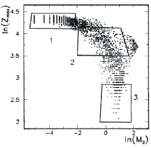
Figure 13: Experimental Campi-scatter-plots from Ref. Mastinu_PRL . Three cuts are employed to selected the upper branch (1), the lower branch (3), and the central region (2).

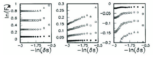
Figure 14: Experimental results from Ref. Mastinu_PRL . Scaled factorial moments ln($F_{k}$) vs -ln($\delta_{s}$) for the three cuts made on Fig. 13: left part cut 1, central part cut 2, and right part cut 3. Solid circles represent the SFM of order k = 2, open circles k = 3, open squares k = 4, and open triangles k = 5. Figure is taken from Ref. Mastinu_PRL .

Actually, several criticisms have been raised about the role of the intermittency signal in nuclear fragmentation. For instance, Elattari et al. showed that an intermittency signal can be obtained even for a simple fragmentation generator model by the random population of mass bins with a power law distribution in which the only non-statistical source of fluctuations is the mass conservation law Elattari . It has also been shown that the intermittency signal is washed out when events of fixed total multiplicity are selected Dorso ; Campi or when the size of the system tends to infinity in the percolation model in which the fluctuations are of nontrivial origin Campi . Moreover, the intermittency signal is not observed in the narrow excitation energy region where the phase transition occurs in the framework of the well-known Copenhagen statistical multi-fragmentation model Barz or in the data of 35-110 MeV/nucleon ${}^{36}Ar+^{197}Au$ when the effects of impact parameter averaging are reduced by some appropriate cuts Phair . However, it is important to notice that there is no reason to expect intermittency if the phase transition is first order.

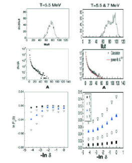
Figure 15: Left panels: the multiplicity distribution (upper panel), the mass distribution (middle panel), the scaled factorial moments (bottom panel) with the multiplicity restriction for ${}^{129}Xe$ in the lattice gas model calculation. Right panel: Same as the left panel but for the events mixed with $T$ = 5.5 MeV and $T$ = 7 MeV. Figure is taken from Ref. Ma_unpub .

As an example, we check the intermittency behavior Ma_unpub in the Lattice Gas model for the disassembly of the system ${}^{129}Xe$ at 0.38$\rho_{0}$ in the framework of LGM (for the details of the model description, please see the following section). At a temperature $T$ = 5.5 MeV, the mass distribution shows a power-law distribution with an effective power-law parameter $\tau$ = 2.43. In a previous work with the same model, it was shown that the liquid-gas phase transition occurs near 5.5 MeV for this system in the LGM Maprc99 ; Ma_PRL . The $lnF_{k}$ shows slight negative values with slightly positive slopes versus $-ln\delta$. However, this kind of the positive slopes with a moment less than unity may be of trivial origin and does not demonstrate the appearance of intermittency which is characteristic of systems exhibiting larger than Poisson fluctuations (i.e. the moment should be larger than unity). In order to check the event mixture effect on the scaled factorial moment, we mixed all the events at $T$ = 4 MeV and $T$ = 7 MeV and also used the multiplicity cuts ($29\leq M\leq 101$) and ($M<29$ or $M>101$) to see if an intermittency behavior can be found in such mixed events. Figure 15 shows these results. Even though all the $lnF_{k}$ values are positive, they are flat, i.e. there is no intermittency signal. In these cases, the fluctuation is large enough but the mass distribution shows no power-law distribution. Hence, intermittency is absent. However, intermittency emerges when the moments were calculated from the mixed events of $T$ = 5.5 MeV and $T$ = 7 MeV (Fig. 15). In this case, the mass distribution shows a quite good power-law distribution and fluctuations are also large enough to induce intermittency.

From the above discussions, the apparent signals of intermittency which emerge in many experimental data are not easy to understand since many experimental conditions bring some complexities to the pure signal of intermittency, such as event mixing. More precise experimental measurements in the future are needed to probe the intermittency signal, which then may be taken as a signal of true critical behavior.

6 Phenomenological Basis of Nuclear Zipf Law and Model Simulation

In the above sections, we have focussed on the moment analysis, namely the behavior of the moments of the fragment size distribution, or of the scaled factorial moments. Both are related to the fluctuations of some physical observables. In this section, we would like to emphasize the topological structure of the fragment size distribution, i.e. how the fragments distribute from the largest to the smallest in nuclear fragmentation. To this end, we introduce the Zipf-type plot, i.e. rank-ordering plot, in the fragment size distribution as well as Zipf’s law which will be illustrated in the following Ma_PRL ; Ma_EPJ .

The original Zipf’s law Crystal has been used for the diagnosis of nuclear liquid-gas phase transition and as such we have called it the nuclear Zipf’s law. Zipf’s law has been known as a statistical phenomenon concerning the relation between English words and their frequency in literature in the field of linguistics Crystal . The law states that, when we list the words in the order of decreasing population, the frequency of a word is inversely proportional to its rank Crystal . This relation was found not only in linguistics but also in other fields of sciences. For instance, the law appeared in distributions of populations in cities, distributions of income of corporations, distributions of areas of lakes and cluster-size distribution in percolation processes soc ; Watanabe . The details for the proposal of nuclear Zipf’s law can been found in Ref. Ma_PRL ; Ma_EPJ . In this report, we firstly define the nuclear Zipf plot for the fragment mass (charge) distribution and nuclear Zipf’s law in the simulation with help of the lattice gas model. Then we show some experimental evidences for the nuclear Zipf law as well as some remarks.

The tools we will use here are the isospin dependent lattice gas model (LGM) and molecular dynamical model (MD). The lattice gas model was developed to describe the liquid-gas phase transition for atomic systems by Lee and Yang Yang52 . The same model has already been applied to nuclear physics for isospin symmetrical systems in the grandcanonical ensemble Biro86 with a sampling of the canonical ensemble Maprc99 ; Camp97 ; Jpan96 ; Mull97 ; Jpan95 ; Jpan98 ; Gulm98 , and also for isospin asymmetrical nuclear matter in the mean field approximation Sray97 . In addition, a classical molecular dynamical model is used to compare its results with the results of the lattice gas model.

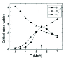
Figure 16: Effective power-law parameter, $\tau$, second moment of the cluster distribution, $S_{2}$, and multiplicity of intermediate mass fragments, $N_{imf}$ as a function of temperature for the disassembly of ${}^{129}Xe$ at $\rho_{f}\sim 0.38\rho_{0}$ in I-LGM. The arrow represents the estimated temperature of the phase transition. Figure is taken from Ma_EPJ .

In the lattice gas model, $A$ (= $N+Z$) nucleons with an occupation number $s$ which is defined $s$ = 1 (-1) for a proton (neutron) or $s$ = 0 for a vacancy, are placed on the $L$ sites of the lattice. Nucleons in the nearest neighboring sites interact with an energy $\epsilon_{s_{i}s_{j}}$. The hamiltonian is written as $E=\sum_{i=1}^{A}\frac{P_{i}^{2}}{2m}-\sum_{i<j}\epsilon_{s_{i}s_{j}}s_{i}s_{j}$. A three-dimension cubic lattice with $L$ sites is used. The freeze-out density of disassembling system is assumed to be $\rho_{f}$ = $\frac{A}{L}\rho_{0}$, where $\rho_{0}$ is the normal nuclear density. The disassembly of the system is to be calculated at $\rho_{f}$, beyond which nucleons are too far apart to interact. Nucleons are put into lattice by Monte Carlo Metropolis sampling. Once the nucleons have been placed we also ascribe to each of them a momentum by Monte Carlo samplings of a Maxwell-Boltzmann distribution. Once this is done the LGM immediately gives the cluster distribution using the rule that two nucleons are part of the same cluster if $P_{r}^{2}/2\mu-\epsilon_{s_{i}s_{j}}s_{i}s_{j}<0$. This method is similar to the Coniglio-Klein prescription Coni80 in condensed matter physics and was shown to be valid in LGM Camp97 ; Jpan96 ; Jpan95 ; Gulm98 . In addition, to calculate clusters using MD we propagate the particles from the initial configuration for a long time under the influence of the chosen force. The form of the force is chosen to compare with the results of LGM. The system evolves with the potential. At asymptotic times the clusters are easily recognized. Observables based on the cluster distribution in both models can now be compared. In the case of proton-proton interactions, the Coulomb interaction can also be added separately and it can be compared with the case without Coulomb effects.

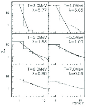
Figure 17: Average charge $Z_{n}$ with rank $n$ as a function of $n$ for ${}^{129}Xe$ $\rho_{f}\sim 0.38\rho_{0}$ in I-LGM. The histograms are the calculation results and the straight lines are their fits with $Z_{n}\propto n^{-\lambda}$. Figure is taken from Ma_EPJ .

In order to check the phase transition behavior in the I-LGM, we will first show the calculations of some physical observables in Fig. 16, namely the effective power-law parameter, $\tau$, the second moment of the cluster distribution, $S_{2}$ Campi , and the multiplicity of intermediate mass fragments, $N_{imf}$, for the disassembly of ¹²⁹Xe at the freeze-out density $\rho_{f}\sim 0.38\rho_{0}$ . These observables have been successfully employed in previous works to probe the liquid- gas phase transition, as shown in Refs. Maprc99 ; Ma_EPJ ; Jpan98 . The valley of $\tau$, the peaks of $N_{imf}$ and $S_{2}$ are located around $T$ $\sim$ 5.5 MeV which is the signature of the onset of the phase transition. Because of the exact mapping between the LGM and the Ising model, we know that at this point the transition is first order.

Now we present the results for testing Zipf’s law in the charge distribution of clusters. The law states that the relation between the sizes and their ranks is described by $Z_{n}=c/n$ (n=1, 2, 3, …), where $c$ is a constant and $Z_{n}$ (or $A_{n}$) is the average charge (or mass) of rank $n$ in a charge (or mass) list when we arrange the clusters in the order of decreasing size. For instance the charge $Z_{2}$ of the second largest cluster with rank $n$ = 2 is one-half of the charge $Z_{1}$ of the largest cluster, the charge $Z_{3}$ of the third largest cluster with rank $n$ = 3 is one-third of the charge $Z_{1}$ of the largest cluster, and so on. In the simulations of this work, we averaged the charges for each rank in charge lists of the events: we averaged the charges for the largest clusters in each event, averaged them for the second largest clusters, averaged them for the third largest clusters, and so on. From the averaged charges, we examined the relation between the charges $Z_{n}$ and their ranks $n$. Figure 17 shows such relations of $Z_{n}$ and $n$ for Xe with different temperatures. The histogram is the simulated results and the straight lines represent the fit with $Z_{n}\propto n^{-\lambda}$ in the range of 1 $\leq$ $n$ $\leq$ 10, where $\lambda$ is the slope parameter. $\lambda$ is 5.77 at $T$ = 3 MeV. Then we increased the temperature and examined the same relation and obtained $\lambda$ = 3.65 and 1.53 at $T$ = 4 and 5 MeV, respectively. Up to $T$ = 5.5 MeV, $\lambda$ = 1.00, i.e., at this temperature the relation is satisfied to the Zipf’s law: $Z_{n}\propto n^{-1}$. When the temperature increases, $\lambda$ decreases; for instance, $\lambda$ = 0.80 at $T$ = 6 MeV and $\lambda$ = 0.56 at $T$ = 7. The temperature at which Zipf’s law emerges is consistent with the phase transition temperature obtained in Fig. 16, illustrating that the Zipf’s law is also an additional signal to determine the location of a phase transition. From a statistical point of view, Zipf’s law could also be related to a critical phenomenon Fisher ; Stauffer . The upper panel of Fig. 18 summarizes the parameter $\lambda$ as a function of temperature.

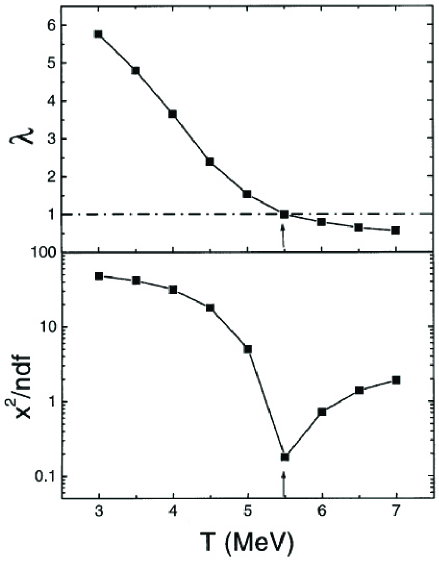
Figure 18: Slope parameter $\lambda$ of $Z_{n}$ to $n$ (top) and $\chi^{2}$ test for Zipf’s law (bottom) as a function of temperature for ${}^{129}Xe$ at $\rho_{f}\sim 0.38\rho_{0}$. The arrow represents the estimated temperature of the phase transition. Figure is taken from Ma_EPJ .

In order to further illustrate that Zipf’s law is most probably fulfilled in phase transition points, we directly reproduce the histograms with Zipf’s law: $Z_{n}=c/n$. In this case, $c$ is the only parameter, but what we are interested in is to check the hypothesis of Zipf’s law through a $\chi^{2}$ test. The bottom panel of Fig. 18 shows the $\chi^{2}/ndf$ for the $Z_{n}$ - $n$ relations at different $T$. As expected, the minimum $\chi^{2}/ndf$ is observed around the phase transition temperature, which further indicates that Zipf’s law of the fragment distribution occurs around the liquid-gas phase transition point.

7 Experimental Evidences of Nuclear Zipf Law

7.1 NIMROD results

In Sec. 4.2, we gave some information on critical behaviors for the Texas A&M NIRMOD data based on the moment analysis technique . Different signals of critical behavior coherently pointing to the same excitation energy interval have been shown. In this section, we will further show the significance of the 5-6 MeV region in NIMROD data using a Zipf’s law analysis. In Fig. 19 we present Zipf plots for rank ordered average $Z$ in six different energy bins. The lines in the figure are fits to the power law expression $\langle Z_{n}\rangle\propto n^{-\lambda}$. Figure 10(f) shows the fitted Zipf exponent, $\lambda$ parameter, as a function of excitation energy. As shown in Fig. 19, this rank ordering of the observation probability of fragments of a given atomic number, from the largest to the smallest, does indeed lead to a Zipf’s power law parameter $\lambda$ = 1 in the 5-6 MeV/nucleon range. Around this excitation energy, the mean size of the second largest fragment is 1/2 of that of the largest fragment; that of the third largest fragment is 1/3 of the largest one, etc. This is a special kind of size topology of fragment distributions, which is very different from the equal-size fragment distribution expected if fragments are formed through a spinodal instability inside the phase coexistence region Borderie-WCI ; Ber ; spin1 ; spin2 ; Colo ; Bord . This shows the relevance of using Zipf-plots to explore the fragment size topology.

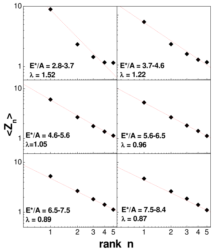
Figure 19: Zipf plots in six different excitation energy bins for the QP formed in ⁴⁰Ar + ⁵⁸Ni. The dots are data and the lines are Zipf-law fits. The statistical error is smaller than the size of the symbols.

7.2 CERN Emulsion Experiment

The nuclear Zipf-type plot has been also applied in the analysis of CERN emulsion or Plastic data of Pb + Pb or Plastic at 158 AGeV following Ma’s proposal on Zipf law, and it was found that the nuclear Zipf law is satisfied in coincidence with other proposed signals of phase transition Poland1 ; Poland2 .

Dabrowska et al. have extended these studies to the multifragmentation of lead projectiles at an energy of 158 AGeV Poland1 . The analyzed data were obtained from the CERN EMU13 experiment in which emulsion chambers, composed of nuclear target foils and thin emulsion plates interleaved with spacers, allow for precise measurements of emission angles and charges of all projectile fragments emitted from Pb-Nucleus interactions. The results on fragment multiplicities, charge distributions and angular correlations are analyzed for multifragmentation of the Pb projectile after an interaction with heavy (Pb) and light (Plastic - $C_{5}H_{4}O_{2}$) targets. A detailed description of the emulsion experiment can be found in Ref. Poland1 .

Figure 20 shows the Zipf-type plot for charged fragments heavier than helium emitted in multifragmentation events of Au or Pb projectile at different beam energies. The values of $\lambda$ exponents from fits $\langle Z_{n}\rangle\sim n^{-\lambda}$ are 0.92 $\pm$ 0.03, 0.90 $\pm$ 0.02 and 0.96 $\pm$ 0.04 for beam energies of 158, 10.6 and 0.64 AGeV, respectively. Within the statistical errors, the values of the $\lambda$ coefficient are the same in the studied energy interval ( $<$ 1-158) AGeV and do not differ significantly from unity Poland1 .

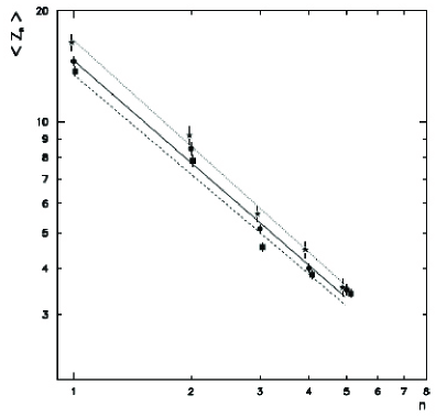
Figure 20: Zipf law fit to the dependences of the mean charge of the fragment on its rank. The different symbols represent the multifragmentation data of different beams with an emulsion target. Circles and solid line represent Pb beam at 158 AGeV, squares and dashed line represent Au beam at 10.6 AGeV, star and dotted line represent Au beam at 0.64 AGeV. Data are taken from Ref. Poland1 .

Dabrowska et al. also studied the dependence of the power law exponent $\lambda$ on the control parameter $m$, the normalized multiplicity with respect to the total charge of spectator particles Poland2 . In Fig. 21(a) are shown the mean multiplicity $\langle N_{f}\rangle$ of fragments with $Z\geq 3$ and the mean number $\langle N_{IMF}\rangle$ of the intermediate fragments. The latter are usually defined as fragments with 3 $\leq Z\leq 30$. In Fig. 21(b) the dependence of the exponent $\tau$ of the power fits to the charge distribution of fragments, performed at different ranges of $m$, is also given. In this analysis, the fits are restricted to fragment charges smaller than $Z=16$. At small values of $m$, a system has few light fragments and the power law is steep; at large values of $m$ there are basically only many light fragments leading again to a steep power law. At the moderate excitation energies where heavier fragments appear and where we expect the phase transition, the exponent $\tau$ has its lowest value. As it can be seen from Fig. 21(b), the minimum $\tau$ occurs for $m$ values between 0.35 and 0.55. In Fig. 21(c) the dependence of $\lambda$ obtained from the fits $\langle Z_{n}\rangle\sim n^{-\lambda}$, as a function of $m$ is depicted. The exponent $\lambda$ decreases with increasing $m$. Between $m\approx 0.3$ and $m\approx 0.5$ the value of $\lambda$ is close to unity and Zipf’s law is satisfied. This suggests that at this value of $m$ the liquid-gas phase transition might occur. It has been checked that $\lambda\sim 1$ occurs in the same region of $m$ irrespectively of the mass of the target Poland2 . This means that the liquid-gas phase transition occurs when a given amount of energy is deposited into the nucleus and does not depend on the mass of the target. As expected, in the case of a liquid-gas phase transition, the previously shown maxima in frequency distributions of multiply charged fragments (Fig. 21(a) ) as well as a minimum of the power law parameter $\tau$ (Fig. 21(b) ), all occur at the same values of $m$, where Zipf’s law emerges.

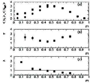
Figure 21: (a) Mean number, $\langle N_{f}\rangle$, of fragments (squares) and mean number, $\langle N_{IMF}\rangle$, of intermediate mass fragments (circles) as a function of the normalized multiplicity m. Error bars are smaller than the size of the squares and circles. (b) Power law exponent, $\tau$, of the charge distribution of fragments in different intervals of m. (c) Power law exponent, $\lambda$, in the Zipf’s law (see text) in different intervals of m. Error bars are smaller then data points. The data is taken from Ref. Poland2 .

7.3 Some Remarks on Zipf Law

Campi et al. pointed out that for an infinite system, Zipf’s law is a mathematical consequence of a power law cluster size distribution with exponent $\tau\simeq 2$ Campi-Zipf . More precisely, both Zipf law exponent $\lambda$ and Fisher scaling power-law exponent $\tau$ are connected through the formula $\lambda=1/(\tau-1$) in an infinite system assuming that the cluster size distribution is a power-law distribution. They argued that such distributions appear at the critical point with $\tau\simeq 2$ of many theories, eg. various theories of cluster formation but also in the super-critical region of the lattice-gas and realistic Lennard-Jones fluids Sator . However, the experimental fragment size distribution is mostly neither power law distribution nor exponential distribution except for some special situations. Also, the nuclear system is always a finite system, which means that the relationship between $\lambda$ and $\tau$ mentioned above is not strictly valid. To account for finite size effects, Bauer et al. Bauer_Zipf have evaluated the fragment probabilities as a function of their rank at the critical point for a finite system with fragment distributions obeying to a finite size scaling ansatz. From this analytical evaluation, where however the assumption is made that all fragments including the largest are much smaller than the source, they suggest to extend the simple Zipf’s law to a more general Zipf-Mandelbrot distribution mandel1 ; mandel2 , $\langle A_{r}\rangle=c(r+k)^{-\lambda}$, where the offset $k$ is an additional constant that one has to introduce, and $\lambda$ is asymptotically approximated as a function of the critical exponent $\tau$, $\lambda=1/(\tau-1)$ of the infinite system.

In any case, the Zipf-type plot is a direct observable allowing to characterize the fragment hierarchy in nuclear disassembly, and as such it is a useful signal of phase transition or critical behavior.

8 Summary and Outlook

In summary, the moment analysis method has been introduced and some applications to nuclear multifragmentation have been presented. Since we are dealing with a finite nucleus rather than infinite nuclear matter, finite size effects must always be discussed in the model calculations and data analysis. Experimentally, the critical behavior of nuclear disassembly can be investigated with the help of moment analysis. The occurrence of a fluctuation peak which can be extracted from the moment analysis method can be interpreted as a signal of critical behavior. Using the same analysis method as for the percolation model, the liquid-gas universality class exponents are approximately obtained in nuclear multifragmentation, such as in EOS data and NIMROD data. This would point to the observation of the liquid-gas critical point or second order phase transition. However, when we think about the system size dependence of critical exponents and we consider some results using Lattice Gas Model simulations and other related different analysis methods, it appears that some open questions still remain concerning the order of the phase transition. For instance, EOS Collaboration claimed that there are continuous phase transitions for heavier systems, namely Au and La and first order phase transitions for lighter system, namely Kr. On the other hand, NIMROD data show critical behavior, corresponding to a continuous phase transition, for the light system Quasi-Ar. Different conclusions are then reached for similar light systems. Recent systematic analyses of caloric curves JBN0 ; Ma2005 ; JBN-WCI and configurational energy fluctuations Gul-WCI , indicate that heavier systems may undergo a first order phase transition while lighter systems can probably sustain a higher temperature, possibly even above the critical point, which would make the first order phase transition observed in heavy nuclei become a cross-over in lighter systems. Concerning configurational energy fluctuations, a well pronounced peak at an excitation energy around 5 MeV was shown in Multics, Indra, Isis and Nimrod data Gul-WCI . However, this fluctuation appears monotonically decreasing in EOS data SrivastavaPRC65 . Thus it deserves further investigations.

Scaled factorial moments and intermittency have also been reviewed and some examples given to show the apparent intermittency in nuclear fragmentation. However, some complex ingredients in experimental measurements, such as mixtures of event multiplicities or temperature fluctuations in the data can induce spurious intermittency-like behavior which implies that the apparent ”intermittency” can not be taken as a unique signal of the critical behavior. Without 4$\pi$ detector upgrades allowing better data sorting, it remains difficult to take apparent ”intermittency” behaviors as a signal of critical behavior in nuclear multifragmentation.

Finally, nuclear Zipf-type plots are introduced and Zipf’s law is proposed to be related to a phase transition or a critical behavior of nuclei. Around the transition point, the cluster mass (charge) shows inversely to its rank, i.e. Zipf’s law appears. Even though the criterion is phenomenological, it is a simple and practicable tool to characterize the fragment hierarchy in nuclear disassembly. The 4$\pi$ multifragmentation data of heavy ion collision at Texas A$\&$M University and the CERN emulsion/plastic data exhibit the Zipf law around the same excitation energy deposit. The satisfaction of the Zipf law for the cluster distributions illustrates that the clusters obey at this point a particular rank ordering distribution very different from the equal-size fragment distribution which may occur due to spinodal instability inside the liquid-gas coexistence region. To conclude, we should mention that all these transition signals, such as the fluctuation peak, critical exponents, Fisher scaling as well as Zipf’s law etc may not be very robust individually since we are facing a transient finite charged nuclear system. A unique signal can not give any definite information as to whether the system is in a critical point or is undergoing a phase transition. Only many coherent signals emerging together can corroborate the observation of a phase transition or a critical behavior in finite nuclei.

This work was supported in part by the Shanghai Development Foundation for Science and Technology under Grant Number 05XD14021, the National Natural Science Foundation of China under Grant Nos. 19725521, 10328259, 10135030, 10535010 and the Major State Basic Research Development Program under Contract No G200077404.

References

- (1) C.A. Ogilvie et al., Phys. Rev. Lett. 67, 1214 (1991); M.B. Tsang et al., Phys. Rev. Lett. 71, 1502 (1993); Y.G. Ma and W.Q. Shen, Phys. Rev. C 51, 710 (1995).
- (2) M.E. Fisher, Physics (N.Y.) 3, 255 (1967).
- (3) S. Albergo, S. Costa, E. Costanzo, A. Rubbino, Nuovo Cimento 89A, 1 (1985).
- (4) J. Pochodzalla et al., Phys. Rev. Lett. 75, 1040 (1995).
- (5) Y.G. Ma et al., Phys. Lett. B 390, 41 (1997).
- (6) J.B. Natowitz et al., Phys. Rev. C 65, 034618 (2002).
- (7) J.B. Natowitz, K. Hagel, Y.G. Ma, M. Murray, L. Qin, R. Wada, and J. Wang, Phys. Rev. Lett. 89, 212701 (2002).
- (8) W. Bauer, Phys. Rev. C 38, 1297 (1988).
- (9) M.L. Gilkes et al., Phys. Rev. Lett. 73, 1590 (1994).
- (10) M. D’Agostino et al., Nucl. Phys. A 650, 329 (1999).
- (11) J.B. Elliott et al., Phys. Rev. C 55, 1319 (1997).
- (12) J.B. Elliott et al., Phys. Rev. C 49, 3185 (1994).
- (13) M. Kleine Berkenbusch, W. Bauer, K. Dillman, S. Pratt, L. Beaulieu, K. Kwiatkowski, T. Lefort, W.C. Hsi, V.E. Viola, S.J. Yennello, R.G. Korteling, and H. Breuer, Phys. Rev. Lett. 88, 022701 (2002).
- (14) Y.G. Ma et al. (NIMROD Collaboration), Phys. Rev. C 69, 031604(R) (2004); Phys. Rev. C 71, 054606 (2005).
- (15) J. Richert and P. Wagner, Phys. Rep. 350, 1 (2001).
- (16) S. Das Gupta, A.Z. Mekjian, M.B. Tsang, Adv. Nucl. Phys. 26 , 89 (2001).
- (17) A. Bonasera, M. Bruno, C.O. Dorso, P.F. Mastinu, Riv. Del Nuovo. Cim. 23, 1 (2000).
- (18) Ph. Chomaz, Proc. of the Int. Nucl. Phys. Conf. INPC2001, Berkeley CA, USA, 2001, ed. by E. Norman, L. Schroeder, G. Wozniak, AIP Conference Proceedings V. 610 (Melville, New York 2002), p. 167.
- (19) L.G. Moretto, J.B. Elliott, L. Phair, G.J. Wozniak, C.M. Mader, and A. Chappars, ibid. p. 182.
- (20) A. Kelic, J.B. Natowitz, K.-H. Schmidt, Contribution to this volume.
- (21) V.E. Viola, R. Bougault, Contribution to this volume.
- (22) B. Borderie, P. Désesquelles, Contribution to this volume.
- (23) F. Gulminelli, M. D’Agostino, Contribution to this volume.
- (24) O. Lopez, M.F. Rivet, Contribution to this volume.
- (25) X. Campi, J. Phys. A 19, L 917 (1986).
- (26) X. Campi, Phys. Lett. B208, 351 (1988).
- (27) W. Bauer et al., Phys. Lett. 150 B, 53 (1985).
- (28) W. Bauer et al., Nucl. Phys. A 452, 699 (1986).
- (29) D. Stauffer, Introduction to Percolation Theory, (Taylor and Francis, London 1985).
- (30) K. Binder, Monte Carlo Methods in Statistical Mechan- ics, 2nd ed. (Springer-Verlag, Berlin 1986).
- (31) H.R. Jaqaman and D.H.E. Gross, Nucl. Phys. A 524, 321 (1991).
- (32) N. Tan et al., Phys. Rev. B 29, 6354 (1984).
- (33) B.K. Srivastava et al., Phys. Rev. C 64, 041605 (2001); Phys. Rev. C 65, 054617 (2002).
- (34) R.P. Scharenberg et al., Phys. Rev. C 64, 054602 (2001).
- (35) J.A. Hauger et al., Phys. Rev. C 57, 764 (1998).
- (36) J.A. Hauger et al., Phys. Rev. C 62, 024616 (2000).
- (37) D. Cussol et al., Nucl. Phys. A 561, 298 (1993).
- (38) J. Lauret et al., Phys. Rev. C 62, R1051 (1998).
- (39) W. Bauer and W.A. Friedman, Phys. Rev. Lett. 77, 767c (1995).
- (40) M.L. Gilkes et al., Phys. Rev. Lett. 77, 768c (1995).
- (41) J.B. Elliott et al., Phys. Rev. C 67, 024609 (2003).
- (42) X. Campi and H. Krivine, Nucl. Phys. A 545, 161c (1992).
- (43) X. Campi and H. Krivine, Z. Phys. A 344, 81 (1992).
- (44) Y.G. Ma et al., Nucl. Phys. A 749, 106c (2005) .
- (45) C.O. Dorso, V.C. Latora, and A. Bonasera, Phys. Rev. C 60, 034606 (1999).
- (46) R. Botet, M. Ploszajczak, A. Chbihi, B. Borderie, D. Durand, and J. Frankland, Phys. Rev. Lett. 86, 3514 (2001).
- (47) Y.G. Ma, J. Phys. G 27, 2455 (2001).
- (48) A. Bialas, R. Peschanski, Nucl. Phys. B 273, 703 (1986).
- (49) B. Mandelbrot, J. Fluid Mech. 62, 331 (1974); U. Frisch, P. Sulem, and M. Nelkin, J. Fluid Mech. 87, 719 (1978).
- (50) Ya. B. Zeldovich et al., Sov. Phys. Usp. 30, 353 (1987).
- (51) G. Paladin and V. Vulpiani, Phys. Rep. 156, 147 (1987).
- (52) A. Bialias and R.C. Hwa, Phys. Lett. B 207, 59 (1988).
- (53) R.C. Hwa and M.T. Nazirov, Phys. Rev. Lett. 69, 741 (1992).
- (54) H. Satz, Nucl. Phys. B326, 613 (1989).
- (55) M. Ploszajczak and A. Tucholski, Phys. Rev. Lett. 65, 1539 (1999).
- (56) L. Phair et al., Phys. Rev. Lett. 79, 3538 (1996); Phys. Lett. B 291, 7 (1992).
- (57) B. Elattari, J. Richert, P. Wagner, Phys. Rev. Lett. 69, 45 (1992); ibid, Nucl. Phys. A 560, 603 (1993).
- (58) H. W. Barz et al., Phys. Rev. C 45, R2541 (1992).
- (59) V. Latora, M. Belkacem, A. Bonesera, Phys. Rev. Lett. 73, 1765 (1994); M. Belkacem, V. Latora, A. Bonasera, Phys. Rev. C 52, 271 (1995).
- (60) X. Campi and H. Krivine, Nucl. Phys. A 589, 505 (1995).
- (61) P.F. Mastinu et al., Phys. Rev. Lett. 76, 2646 (1996).
- (62) Y.G. Ma, unpublished.
- (63) Y.G. Ma et al., Phys. Rev. C60, 024607 (1999).
- (64) Y.G. Ma, Phys. Rev. Lett. 83, 3617 (1999).
- (65) Y.G. Ma, Eur. Phys. J. A 6, 367 (1999).
- (66) G.K. Zipf, Human Behavior and the Principle of Least Effort, Addisson-Wesley Press, Cambridge, MA, 1949.
- (67) D.L. Turcotte, Rep. Prog. Phys. 62, 1377 (1999).
- (68) M. Watanabe, Phys. Rev. E 53, 4187 (1996).
- (69) T.D. Lee and C.N. Yang, Phys. Rev. 87, 410 (1952).
- (70) T.S. Biro et al., Nucl. Phys. A 459, 692 (1986); S.K. Samaddar and J. Richert, Phys. Lett. B 218, 381 (1989); Z. Phys. A 332, 443 (1989); J.M. Carmona et al., Nucl. Phys. A 643, 115 (1998).
- (71) X. Campi and H. Krivine, Nucl. Phys. A 620, 46 (1997).
- (72) J. Pan and S. Das Gupta, Phys. Rev. C 53, 1319 (1996).
- (73) W.F.J. Müller, Phys. Rev. C 56, 2873 (1997).
- (74) J. Pan and S. Das Gupta, Phys. Lett. B 344, 29 (1995); Phys. Rev. C 51, 1384 (1995); Phys. Rev. Lett. 80, 1182 (1998); S. Das Gupta et al., Nucl. Phys. A 621, 897 (1997).
- (75) J. Pan and S. Das Gupta, Phys. Rev. C 57, 1839 (1998).
- (76) F. Gulminelli and Ph. Chomaz, Phys. Rev. Lett. 82, 1402 (1999).
- (77) S. Ray et al., Phys. Lett. B 392, 7 (1997).
- (78) A. Coniglio and E. Klein, J. Phys. A 13, 2775 (1980).
- (79) G. F. Bertsch and P.J. Siemens, Phys. Lett. 126B, 9 (1983).
- (80) L.G. Moretto et al., Phys. Rev. Lett. 77, 2634 (1996).
- (81) L. Beaulieu et al., Phys. Rev. Lett. 84, 5971 (2000).
- (82) M. Colonna et al., Phys. Rev. Lett. 88, 122701 (2002).
- (83) B. Borderie et al., Phys. Rev. Lett. 86, 003252 (2001).
- (84) A. Dabrowska, M. Szarska, A. Trzupek, W. Wolter, B. Bosiek, Acta Phys. Pol. B 32, 3099 (2001).
- (85) A. Dabrowska, M. Szarska, A. Trzupek, W. Wolter, B. Bosiek, Acta Phys. Pol. B 35, 2109 (2004).
- (86) X. Campi and H. Krivine, Phys. Rev. C 72, 057602 (2005).
- (87) N. Sator, Phys. Rep. 376, 1 (2003).
- (88) W. Bauer, B. Alleman, S. Pratt, nucl-th/0512101.
- (89) B. Mandelbrot, An informational theory of the statistical structure of language, in Communication Theory, ed. W. Jackson (Betterworths, 1953).
- (90) B. Mandelbrot, The Fractal Geometry of Nature (Freeman, 1982).