Systematics of pion emission in heavy ion collisions in the $1A$ GeV regime.

Abstract

Using the large acceptance apparatus FOPI, we study pion emission in the reactions (energies in $A$ GeV are given in parentheses): ⁴⁰Ca+⁴⁰Ca (0.4, 0.6, 0.8, 1.0, 1.5, 1.93), ⁹⁶Ru+⁹⁶Ru (0.4, 1.0, 1.5), ⁹⁶Zr+⁹⁶Zr (0.4, 1.0, 1.5), ¹⁹⁷Au+¹⁹⁷Au (0.4, 0.6, 0.8, 1.0, 1.2, 1.5). The observables include longitudinal and transverse rapidity distributions and stopping, polar anisotropies, pion multiplicities, transverse momentum spectra, ratios $(\pi^{+}/\pi^{-})$ of average transverse momenta and of yields, directed flow, elliptic flow. The data are compared to earlier data where possible and to transport model simulations.

, , , , , , , , , , , , , , , , , , , , , , , , , , , , , , , , , , , , , , , , , , , , , , , , ,

(FOPI Collaboration)

1 Introduction

The quest to use energetic heavy ion collisions to infer properties of infinite nuclear matter, such as the equation of state (EOS) under conditions of density (or pressure) and temperature significantly different from the ground state conditions has proven to be a difficult task, although an impressive amount of data has been obtained using experimental setups of increasing sophistication. At incident energies per nucleon on the order or smaller than the rest masses, systems consisting of two originally separated nuclei are small in the sense that surface effects cannot be neglected even if some kind of transient equilibrium situation were achieved.

In particular, the mean free paths of pions [1], [2], the most abundantly created particles, with momenta below 1 GeV/c are neither large nor small compared to typical nuclear sizes. Therefore methods of analysis resting on the validity of either of these two extremes in the hope to simplify the theoretical description are bound to lead only to qualitative success at best. As a result, event simulation codes based on microscopic transport theory were soon developed [3] that allowed for multiple elementary collisions as the heavy ion reaction proceeds, without however requiring a priori full equilibration.

An important lesson that was learned in the last two decades was that definite conclusions on nuclear matter properties based on a single observable had proven to be premature and/or of limited accuracy, aside from not being sufficiently convincing. As an example, original hopes [4],[5] to use deficits in pion production relative to expectations based on compression-free scenarios were not supported by transport theoretical simulations [6], [7], [8].

On the other hand transport calculations [9] showed that pion azimuthal correlations, ’flow’, qualify as an observable that could contribute significant constraints on the EOS. However, as pion production in the 1A GeV regime (at SIS) is not as copious as it is in higher energy regimes and as pion azimuthal correlations turn out to be rather small (an effect of a few percent), it was concluded [9] that ’very high statistics and high-precision impact parameter classification are necessary’ to exploit the sensitivity of pion flow to the EOS.

This requires the need for large acceptance detection systems capable of registering under exclusive conditions a much larger number of events than had been possible with the Berkeley Streamer Chamber that was operated in the 80’s to obtain pion data at the BEVALAC accelerator [10], [11], [12], [4]. The first electronic $4\pi$-detector capable of measuring pions was DIOGENE [13] installed at the Saturne synchrotron in Saclay. The pion emission data presented in this work were obtained with a large acceptance, high granularity device, FOPI [14, 15] installed at the SIS accelerator in Darmstadt. Particle identification is based on time-of-flight, energy loss and magnetic rigidity measurements with use of large volume drift chambers and scintillator arrays. A second large acceptance device [16], based on the use of a time projection chamber, was also operated in the nineties at the BEVALAC accelerator in Berkeley. In addition, more specialized devices were build and used at the SIS accelerator in Darmstadt: KaoS [17], a high resolution magnetic spectrometer and TAPS [18], based on arrays of BaF₂ detectors allowing to identify neutral pions and $\eta$ particles via their two-photon decay branches.

The experimental situation concerning the pion observable before the advent of these newer devices was reviewed in ref. [5], some of the more recent particle production data obtained in the nineties at the SIS accelerator and also at other accelerators (AGS and SPS) covering higher energies have been summarized in ref. [19].

Our Collaboration has published pion data before [20], [21], [22], [23], [24], but these were more limited in scope and, in particular, did not treat pion flow and isospin dependences. Also, we call attention to the fact that the data of ref. [20] (for Au on Au at $1.06A$ GeV) have been revised and should be superseded by the present data (see section 6.1 for details). The aim of the present work is to present a more complete systematics of highly differential pion emission in heavy ion reactions obtained with the FOPI device, varying the incident energy (from 0.4 to $1.9A$ GeV), the system’s size (from $A_{p}+A_{t}=40+40$ to $197+197$, where $A_{p}$ and $A_{t}$, are the projectile and target mass number, respectively) and the system’s isospin, and, of course, the event selection method i.e. the centrality.

After describing the experimental methods we report on the following observables for charged pions of both polarities:

• longitudinal and transverse rapidity distributions and stopping;

• polar anisotropies;

• pion multiplicities;

• transverse momentum spectra;

• ratios $(\pi^{+}/\pi^{-})$ of average transverse momenta and of yields;

• directed flow;

• elliptic flow.

While discussing each of these subjects, we shall refer more explicitly to relevant earlier work and compare data where possible. All along we shall also present the results of simulations with a transport code showing the degree to which our data can be understood on a microscopic level and assessing conditions for equilibration (stopping), sensitivities to assumptions on the EOS and the propagation of pions in the medium and searching for signals that might give information on the isospin dependence of the EOS. While pions present a probe of hot and compressed matter of high interest in its own right, it is also important to have this observable under firm theoretical control as it is a link to understanding the production of strangeness under subthreshold conditions where the pion emitting baryonic resonances are thought to play an essential role in the collision sequences leading to outgoing strange particles, such as kaons. We will end with a summary.

2 Experimental method

The experiments were performed at the heavy ion accelerator SIS of GSI/Darmstadt using the large acceptance FOPI detector [14, 15]. A total of 18 system-energies are analysed for this work (energies in $A$ GeV are given in parentheses): ⁴⁰Ca+⁴⁰Ca (0.4, 0.6, 0.8, 1.0, 1.5, 1.93), ⁹⁶Ru+⁹⁶Ru (0.4, 1.0, 1.5), ⁹⁶Zr+⁹⁶Zr (0.4, 1.0, 1.5), ¹⁹⁷Au+¹⁹⁷Au (0.4, 0.6, 0.8, 1.0, 1.2, 1.5). Particle tracking and energy loss determination are done using two drift chambers, the CDC (covering polar angles between $35^{\circ}$ and $135^{\circ}$) and the Helitron ($9^{\circ}-26^{\circ}$), both located inside a superconducting solenoid operated at a magnetic field of 0.6T. A set of scintillator arrays, Plastic Wall $(7^{\circ}-30^{\circ})$, Zero Degree Detector $(1.2^{\circ}-7^{\circ})$, and Barrel $(42^{\circ}-120^{\circ})$, allow us to measure the time of flight and, below $30^{\circ}$, also the energy loss. The velocity resolution below $30^{\circ}$ was $(0.5-1.5)\%$, the momentum resolution in the CDC was $(4-12)\%$ for momenta of 0.5 to 2 GeV/c, respectively. Use of CDC and Helitron allows the identification of pions, as well as good isotope separation for hydrogen and helium clusters in a large part of momentum space. Heavier clusters are separated by nuclear charge. More features of the experimental method, some of them specific to pions, have been described in Ref. [20].

2.1 Pions: reconstructing $4\pi$ from FOPI

The pion data presented in this work are limited to the CDC. In one of two independent analyses methods, particle tracking was based on the Hough transform method, HT. Track quality cuts were varied systematically and the results extrapolated to zero cuts to achieve estimates of the tracking efficiency. The relative efficiency of positively and negatively charged pions was inferred from studies of the isospin symmetric system ⁴⁰Ca+⁴⁰Ca. An alternative method of data analysis with a local tracker, LT, has also been used allowing extensive cross checking. This method is documented in ref. [25] and we shall briefly come back to it in section 3.

The measured momentum space distributions of pions do not cover the complete $4\pi$ phase space and must be complemented by interpolations and extrapolations. In the HT method, we filter the data to eliminate regions of distorted measurements (such as edge effects) and correct for efficiency where necessary. Since this study is limited to symmetric systems, we require reflection symmetry in the center of momentum ($c.o.m.$). Choosing the $c.o.m.$ as reference frame, orienting the z-axis in the beam direction, and ignoring for the moment deviations from axial symmetry (see section 9) the two remaining dimensions are characterized by the longitudinal rapidity $y\equiv y_{z}$, given by $exp(2y)=(1+\beta_{z})/(1-\beta_{z})$ and the transverse (spatial) component $t$ of the four-velocity $u$, given by $u_{t}=\beta_{t}\gamma$. The 3-vector $\vec{\beta}$ is the velocity in units of the light velocity and $\gamma=1/\sqrt{1-\beta^{2}}$. In order to be able to compare longitudinal and transversal degrees of freedom on a common basis, we shall also use the transverse rapidity, $y_{x}$, which is defined by replacing $\beta_{z}$ by $\beta_{x}$ in the expression for the longitudinal rapidity. The $x$-axis is laboratory fixed and hence randomly oriented relative to the reaction plane, i.e. we average over deviations from axial symmetry. The transverse rapidities $y_{x}$ (or $y_{y}$) should not be confused with $y_{t}$ which is defined by replacing $\beta_{z}$ by $\beta_{t}\equiv\sqrt{\beta_{x}^{2}+\beta_{y}^{2}}$.

For thermally equilibrated systems $\beta_{t}=\sqrt{2}\beta_{x}$ and the local rapidity distributions $dN/dy_{x}$ and $dN/dy_{y}$ (rather than $dN/dy_{t}$) should have the same shape and height than the usual longitudinal rapidity distribution $dN/dy_{z}$, where we will omit the subscript $z$ when no confusion is likely. Throughout we use scaled units $y_{0}=y/y_{p}$ and $u_{t0}=u_{t}/u_{p}$, with $u_{p}=\beta_{p}\gamma_{p}$, the index p referring to the incident projectile in the $c.o.m.$. In these units the initial target-projectile rapidity gap always extends from $y_{0}=-1$ to $y_{0}=1$. It is useful to recall that in non-viscous one-fluid hydrodynamics many observables scale when the system’s size and energy, but not the shape or impact parameter, are varied.

Choosing central collisions of Au on Au at $0.8A$ GeV as a typical example, we show in the upper left panel of Fig. 1 the original $\pi^{-}$ (CDC) data in the $(y_{0}$-$u_{t0})$ plane. Proceeding from the upper left to the lower right panel of the figure, the next two panels show the data after application of a sharp filter and the use of reflection symmetry.

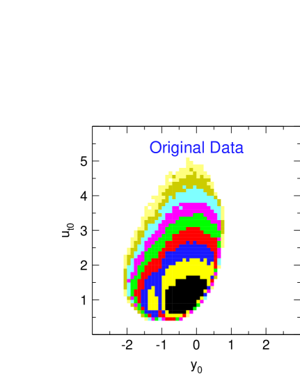
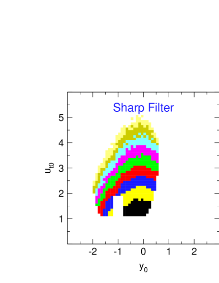
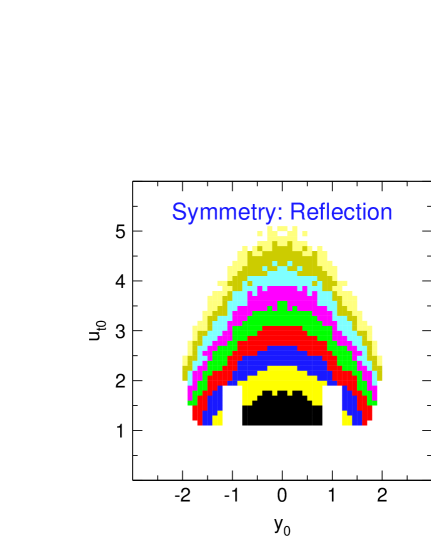
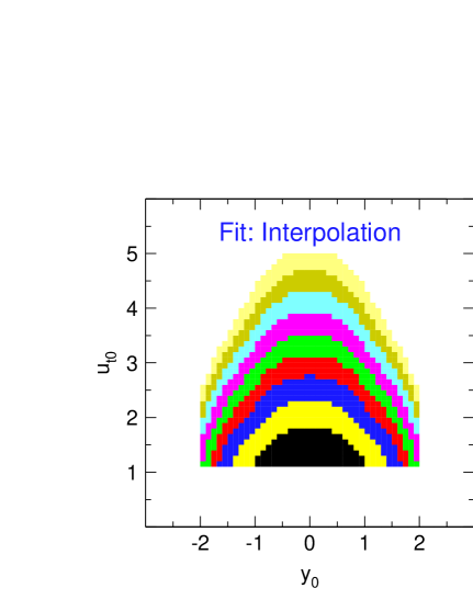
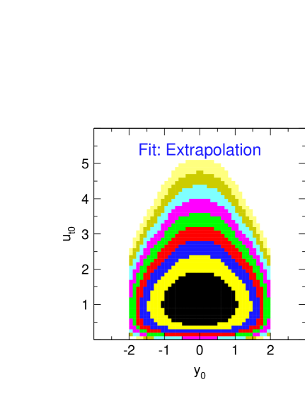
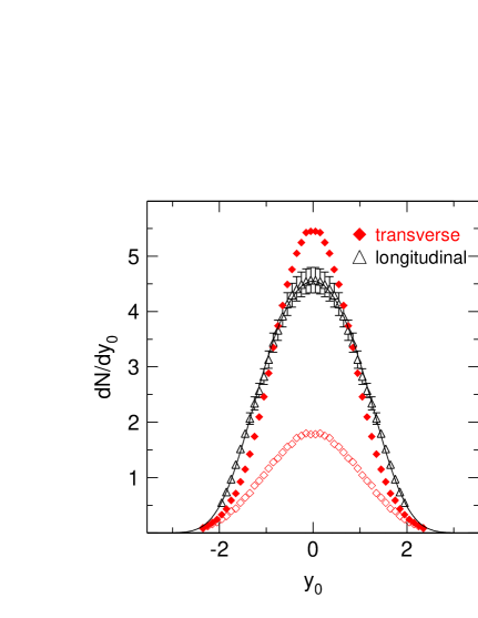
Figure 1: Distributions $dN/du_{t0}dy_{0}$ of pions ($\pi^{-}$) emitted in central collisions of Au on Au at $0.8A$ GeV. The various color tones correspond to cuts differing by factors 1.5. Five panels show the evolution of the data treatment (see text), while the sixth panel (lower right) shows deduced longitudinal and transverse rapidity distributions. The transverse rapidity distribution with a cut on longitudinal rapidity $(|y_{0}|<0.1)$, is also shown.

In the following step each measured phase-space cell $dy_{0}*du_{t0}$ and its local surrounding $N_{yu}$ cells, with $N_{yu}=(2n_{y}+1)(2n_{u}+1)$, is least squares fitted using the ansatz

$$\frac{1}{u_{t0}}\frac{d^{2}N}{du_{t0}dy_{0}}=\exp\,[f(y_{0},u_{t0})]$$

where $f(x,y)=a_{2}x^{2}+b_{2}y^{2}+d|x|y+a_{1}|x|+b_{1}y+c_{0}$ is a five parameter function.

This procedure smoothens out statistical errors and allows subsequently a well defined iterative extension to gaps in the data. Within errors the smoothened representation of the data follows the topology of the original data: typical deviations are $5\%$ i.e. of a magnitude that exceeds statistical errors in most cases and is caused by local distortions of the apparatus response, thus revealing typical systematic uncertainties.

The technical parameters of the procedure were chosen to be $dy_{0}=0.1$, $du_{t0}=0.1$, $n_{y}=4$, $n_{u}=6$ (except for the data at 0.4A GeV where $n_{y}=6$ and $n_{u}=8$). These choices are governed by the available statistics and the need to follow the measured topology within statistical and systematics errors. Variations of these parameters were investigated and found to be uncritical within reasonable limits.

The smoothened data (middle right panel) are well suited for the final step: the extrapolation to zero transverse momenta also shown in the figure (bottom left panel).

The low $p_{t}$ extrapolation procedure was guided by microscopic event simulations (to be described in more detail in section 3) that take into account the influence of Coulomb effects, which differ for the two kinds of charged pions.

Figure 2: Transverse momentum spectrum of negative pions in the reaction Au+Au at $0.8A$GeV. The symbols represent data from a simulation with IQMD SM. The solid line is a least squares fit (see text) using the data in the momentum range (marked ’adjust’) from 0.1 to 0.25 GeV/c.

Figure 3: The power parameter used to reproduce the simulated data for positive and negative pions as a function of the size (total charge) of the system.

Fig. 3 shows a simulated transverse momentum spectrum for $\pi^{-}$ emitted in central Au on Au collisions at 0.8A GeV. It is integrated over all longitudinal rapidities. The range to be extrapolated for the experimental data ($p_{t}<0.1$ GeV/c) is indicated. The simulated data were fitted in the indicated adjustment range (0.1-0.25 GeV/c) with the function

$$N\exp(-p_{t}^{x}/c)$$

the power $x$ and the constant $c$ being two shape parameters, and $N$ a normalization parameter (in the non-relativistic, no-Coulomb regime a ’thermal’ fit would mean $x=2.0$ and $c=2mT$ in terms of a temperature $T$). The fit function was accepted when it also gave a good reproduction of the theoretical data in the low-$p_{t}$ range (even though it was not included in the fitting procedure). The best powers $x$, shown in Fig. 3, turned out to be somewhat lower than 2, depending on the system size and the pion charge polarity. The dependence on the incident energy was very weak and therefore was ignored.

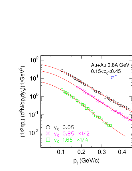
Figure 4: Measured transverse momentum spectra of $\pi^{-}$ in the reaction Au+Au at $0.8A$ GeV in various scaled rapidity bins of widths 0.1. Centroids and data scaling factors are given in the figure. The data are given by symbols, the solid lines represent a smoothened version of the data plus extrapolations.

The experimental data were then extrapolated using the same (available) adjustment range and $x$-values suggested by the simulation but varying $N$ and one shape parameter only, $c$. The typical outcome is shown in Fig. 4 for three indicated scaled rapidity intervals.

2.2 Centrality selection

Collision centrality selection was obtained by binning distributions of the ratio, $ERAT$ [26], of total transverse and longitudinal kinetic energies. In terms of the scaled impact parameter, $b_{0}=b/b_{max}$, we choose the same centralities for all the systems: $b_{0}<0.15$ (i.e. $2.25\%$ in terms of total cross sections), $b_{0}<0.25$, $0.25<b_{0}<0.45$, $0.45<b_{0}<0.55$. We take $b_{max}=1.15(A_{P}^{1/3}+A_{T}^{1/3})$ fm as effective sharp radius and estimate $b$ from the measured differential cross sections for the $ERAT$ distribution using a geometrical sharp-cut approximation. $ERAT$ selections do not imply a priori a chemical bias. Autocorrelations in high transverse momentum population, that are caused by the selection of high $ERAT$ values, are avoided by not including identified pions in the selection criterion.

3 Simulation using the IQMD transport code.

In the present work we are making extensive use of the code IQMD [27] which is based on Quantum Molecular Dynamics [28]. Many interesting predictions and revealing interpretations of the mechanisms involving pions have been made [29]-[34], [9] with this model before our data were available making it almost mandatory to confront it now with the present measured data.

One of the motivations for numerical simulations of heavy ion reactions with transport codes is the possibility to investigate the effect of the underlying equation of state, EOS, on the experimental observables without relying on the restrictive assumption of local (and a fortiori global) equilibrium followed by ’sudden’ freeze-out of all elementary hadronic collisions. In between collisions, nucleons are propagating in mean fields, the nuclear parts of which correspond in the limit of infinite matter to well defined zero temperature EOS. These EOS can be chosen to be ’stiff’ or ’soft’, as characterized in terms of incompressibilities $K=380$ MeV, respectively 200 MeV, where $K=9\rho^{2}\partial^{2}(E/A)/\partial\rho^{2}$ near $\rho=\rho_{0}$, the saturation density. We shall henceforth label these two options, HM, respectively SM. The M in HM and SM stands for the momentum dependence of the nucleon-nucleon interaction. IQMD incorporates a phenomenological Ansatz fitted to experimental data on the real part of the nucleon-nucleus optical potential. In the IQMD code pions are produced by the decay of the 1232 MeV $\Delta$ baryon resonance and may be reabsorbed exclusively by forming a $\Delta$ again. The dominance of the lowest nucleonic excitation in the $1A$ GeV energy regime has been directly demonstrated in proton-pion correlation studies [35], [36], [37].

While in between collisions, the $\Delta$ baryons are propagating in the same nuclear and Coulomb fields as the nucleons, pions are feeling only the Coulomb potential. For simplicity, and in order to limit the number of input variables we ’shut off’ the poorly known (isospin) symmetry potential in these exploratory calculations. Thus ’isospin effects’, if any, would have to result either from the isospin dependent NN cross sections (implemented in the code), e.g. a ’cascade’ effect, and/or the Coulomb fields. As in the model pion production and absorption is strongly connected with $\Delta$ baryon production and absorption, the physics of $\Delta$ propagation in the medium becomes important both for the observed final number of pions and the flow pion ’daughters’ inherit from their ’parents’. If not otherwise stated we have used in our calculations the scheme of ref. [8] for the $\Delta$ baryon mass distribution and width.

Some recent implementations of transport theoretical codes for heavy ion collisions in the $1A$ GeV regime contain more advanced features than those just described. Without attempting to be complete, we mention the works of Bao An Li and coworkers [38] and of the Catania group [39] which implement various isospin dependences of the mean field. Other codes have made progress implementing non-equilibrium aspects of the local densities [40], better accounting for off-shell effects when particle (resonance) lifetimes are short and/or the collision rate is high [41], reassessing the in-medium cross sections for the $NN\rightarrow N\Delta$ reaction [42], etc. . The code of Danielewicz [43] includes nucleonic clusters up to mass three and has been used in our context here to clarify the role of expansion on the pion observables. Very recently, the relativistic code UrQmd has also been used [44] to study SIS energy reactions, although its original design [45] was directed towards much higher energies. Most of these codes include the influence of many higher baryonic resonances.

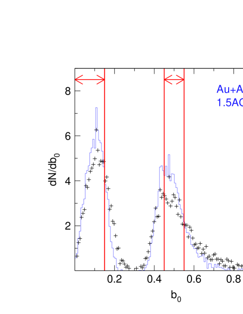
Figure 5: Simulated reduced impact parameter distributions for Au+Au collisions at $1.5A$ GeV using the global observable $ERAT$ for event selection. The two peaks correspond to nominal centralities $b_{0}<0.15$ and $0.45<b_{0}<0.55$, respectively, as indicated by the vertical lines and the double arrows. Histograms (crosses) correspond to unfiltered (filtered) data.

One of the advantages of a QMD type code over BUU (Boltzmann-Uehling-Uhlenbeck) implementations might be its capability to induce finite (nucleon) number fluctuations without resorting to additional assumptions or recipes. For the simulation of the experimental situation it is of paramount importance that there is an accurate ’centrality matching’. i.e. the centrality criterion of the experiment (here the observable $ERAT$) and its realistic fluctuations should be simulated. We vary $b_{0}$ uniformly between 0 and 1 and add the events (about 50000 per system-energy) weighed by $b_{0}$. Fig. 5 shows $b_{0}$ distributions resulting from $ERAT$ selection in two of our standard centrality intervals. The nominal $b_{0}$ intervals are also shown, as well as the effect of applying a filter that takes into account the geometrical and the threshold limits of the apparatus. As can be seen this filter does not have a dramatic influence on the distributions, and hence its details are not critical. However, the effect of using $ERAT$, rather than the experimentally elusive $b_{0}$, is not negligible, even with a perfect detector. For the energy range of interest here, we find that the alternative selection method, binning charged particle multiplicities, yields less sharp $b_{0}$ distributions as long as $b_{0}<0.40$, but is competitive for more peripheral collisions. In particular, multiplicity binning avoids the high $b_{0}$ tails beyond $b_{0}=0.6$ visible in the figure. Multiplicity selected data are available, but will not be shown here. $ERAT$ has the advantage that it does not require the simulation to reproduce the degree of nucleonic clusterization, a difficult (still) task for transport codes (see ref. [46]). Finite number effects deteriorate the $b_{0}$ ’resolution’ when lighter systems, such as Ca+Ca, are studied, an additional reason to try to be realistic when simulating the experiment.

We have also used the IQMD code with a more technical aim: we have introduced it [25] as an event generator for a GEANT based [47] Monte Carlo simulation of our apparatus response to better assess tracking efficiencies and losses due to geometrical limitations. This alternative independent data analysis [25] using a local tracking method, LT, instead of the Hough-transform based tracker, HT, was found to yield $4\pi$ pion multiplicities in good agreement ($10\%$ or better) with the method outlined above (e.g. see Figs. 17 and 20 in section 6).

4 Rapidity distributions and stopping

Before looking at special projections in momentum space it is useful to display the full (2-dimensional) distributions $dN/du_{t0}dy_{0}$. One such distribution was already shown in Fig. 1 for Au+Au at $0.8A$ GeV. To see the evolution of the topology with incident energy - i.e. from $0.4A$ to $1.5A$ GeV - two more such distributions are shown in the upper panels of Fig. 6.

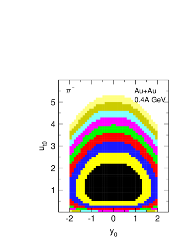
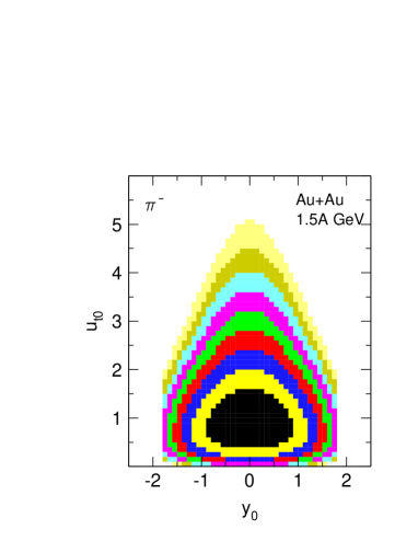
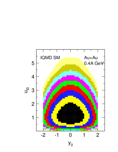
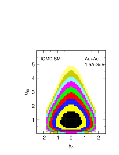
Figure 6: $dN/du_{t0}dy_{0}$ distributions for pions $(\pi^{-})$ emitted in $b_{0}<0.15$ collisions of Au+Au at $0.4A$ GeV (left) and $1.5A$ GeV (right). Top panels: data, bottom panels: simulation. The grey (color) tones differ by factors 1.5.

The pion (here $\pi^{-}$) sources are centered at midrapidity with no readily evident memory of the initial conditions (i.e. around $|y_{0}|=1$). Comparing the contours at $0.4A$ GeV with those at $1.5A$ GeV, one notices that in the scaled units chosen for these plots, the distributions are significantly wider in both dimensions at the lower energy. The data at $0.4A$ GeV span more than twice the full rapidity gap. At least two properties involved in pion production are not expected to scale: a) the nucleonic Fermi motion which should be relatively more important at the lower energy and b) the decay kinematics of the parent $\Delta$ (and other) baryonic resonances.

The simulation with IQMD (see the lower panels) qualitatively reproduces the higher ’compactness’ at $1.5A$ GeV, but is less expanded in the longitudinal direction, especially at the lower energy.

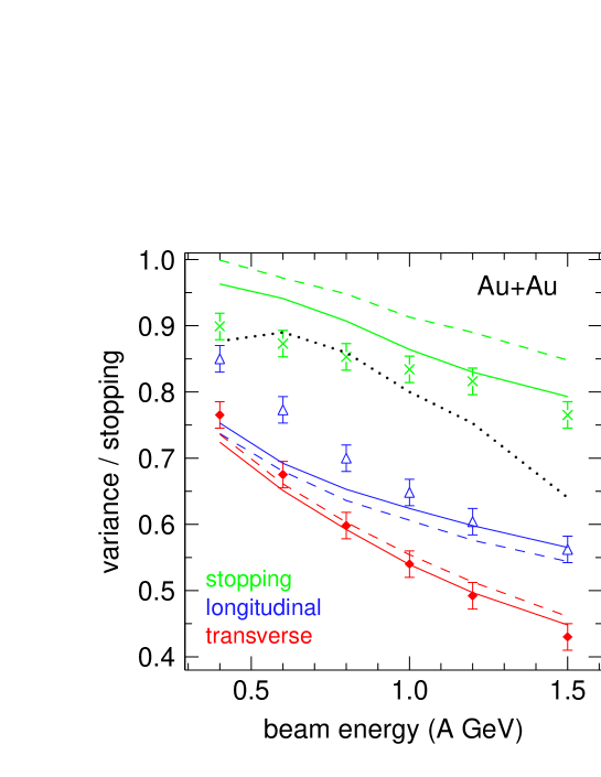
Figure 7: Various excitation functions for $b_{0}<0.15$ collisions of Au+Au. The symbols represent from top to bottom the stopping observable vartl, the variance of the longitudinal rapidity, the variance of the transverse rapidity. The corresponding observables from the IQMD simulation are represented by solid (dashed) lines for SM (HM). The dotted curve is the measured [48] stopping for nucleons.

A more quantitative assessment of these features can be made in terms of longitudinal, $dN/dy_{0z}$, and transverse, $dN/dy_{0x}$, rapidity distributions deduced from the reconstructed $4\pi$ data. Due to apparatus limitations, and in order to keep the technical definition of the scaled variances of these distributions strictly constant over the full range of system-energies and centralities, we define the variances $\sigma^{2}(y_{0z})$, resp. $\sigma^{2}(y_{0x})$, of these distributions in the finite interval $|y_{0}|<1.8$ for pions. Further we define the ratio $vartl=\sigma^{2}(y_{0x})/\sigma^{2}(y_{0z})$ which we shall loosely call ’degree of stopping’ or just ’stopping’. In a non-relativistic purely ’thermal’ interpretation this ratio would represent the ratio of transverse to longitudinal ’temperatures’, which, if different from one, would then imply non-equilibrium. In Fig. 7 we show measured excitation functions for $\sigma^{2}(y_{0z})$, $\sigma^{2}(y_{y0x})$ and of $vartl$ (symbols indicated in the figure).

The scaled variances are seen to decrease significantly and steadily with incident energy, as expected from the qualitative discussion of Fig. 6. The ’pionic stopping’ is consistently below one, but decreases less rapidly with energy. We also include from our earlier work [48] the ’nucleonic stopping’ (dotted) for comparison: it decreases faster with energy than its pionic counterpart. Some of the difference between pions and nucleons results from the fact that the observed pionic momenta result from a convolution of the excited nucleon momenta with the decay kinematics, a convolution that is expected to lead to a more homogeneous (isotropic) final momentum distribution. A more subtle effect would be that different hadrons witness on the average different collision histories in a non-equilibrium situation.

These effects should be taken care of in a microscopic simulation. The solid lines in Fig. 7 are the prediction of IQMD SM which follow the measured transverse variances amazingly well, but show a flatter trend for the longitudinal variances coming closer to the data at the highest energy and underestimating the measured values at the low energy end, confirming again trends seen qualitatively in Fig. 6. As a consequence the ’stopping’ is also overestimated especially at the low energy end. The mean field (SM versus HM) has a modest, but not negligible, influence: the stiffer EOS leads to a general increase of the stopping (uppermost dashed line) by roughly $5\%$ caused by the correlated decrease/increase of the longitudinal/transverse variance.

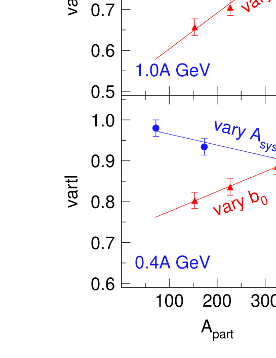
Figure 8: Pion stopping, vartl, as function of the number of participant nucleons, $A_{part}$ for collisions at $1.5A$, $1.0A$ and $0.4A$ GeV (top to bottom). Left panels: data, right panels: IQMD simulation. The two branches correspond to two modes of varying $A_{part}$: 1) central ($b_{0}<0.15$) collisions varying the total system size, marked ’vary $A_{sys}$’, and 2) collisions of Au+Au varying centrality, marked ’vary $b_{0}$’.

Naively, if stopping is incomplete, the degree of stopping is expected to depend on the system’s size characterized by the total number of nucleons, $A_{sys}$. Our data comprise the systems Ca+Ca ($A_{sys}=80$), Ru+Ru ($A_{sys}=192$) and Au+Au ($A_{sys}=394$) where we roughly double the nucleonic size from one system to the next. In order to compare, we keep the centrality in scaled impact parameters constant ($b_{0}<0.15$). In terms of ’participants’ one can also vary the (participant) system size $A_{part}$, by changing the impact parameter $b_{0}$, keeping $A_{sys}$ constant. (In order not to interrupt the flow of arguments here, we refer the reader to section 6 for a definition and discussion of $A_{part}$.) With the concept of participant size, we are then in a position to establish with our data a summary of the pion stopping systematics, based on the two methods just discussed, see Fig. 8 and its caption. In the figure we have plotted averages for both polarities, $\pi^{+}$ and $\pi^{-}$, as no significant difference was observed.

The main message of this systematics (which is reproduced semiquantitatively by the simulation) is that there is no unique dependence on $A_{part}$, but also a dependence on either the shape of the participant volume (which depends on the collision geometry, hence $b_{0}$), or on the presence of more or less ’spectator’ matter in the early stages of the reaction, an interpretation we favour in the present energy regime. The idea is that pions, being fast moving light hadrons (notice in Fig. 6 some pions are seen to freeze out with 4-5 times the incident nucleon velocities $u_{p}$) are able to penetrate into the spectator matter before the latter has left the neighbourhood of the participant zone. These pions are then rescattered experiencing a partial longitudinal reacceleration. This results in a smaller apparent stopping, an effect that increases with the size of the spectator matter, as suggested by Fig. 7. These pion (or $\Delta$ baryon) rescatterings in spectator matter also influence the anisotropies of azimuthal emissions [29, 30] to be discussed later.

5 Anisotropies

In thermal model analyses of pion data (see for example [49]) it is often assumed that pion emission is isotropic in the c.o.m. in order to extend to $4\pi$ the measured mid-rapidity data. However, already early studies [50, 51, 2] of inclusive reactions have reported deviations from isotropy: usually the polar angle distributions have a minimum near $90^{\circ}$ c.o.m.. More recently, the TAPS collaboration has observed [2, 52, 53] anisotropic $\pi^{0}$ emission in asymmetric heavy ion systems at subthreshold energies and interpreted the inclusive data in terms of a ’primordial’ pion emission followed by final state interactions (rescattering and absorption). The averaging over impact parameters and the presence of asymmetrically distributed spectator matter in the chosen reactions complicate the microscopic interpretation of such data. In the present work, the fact that the stopping observable $vartl$ (see previous section) was found to be less than one, indicates that isotropy is not fulfilled even in the most exclusive central collisions, despite minimal amounts of ’shadowing’ spectator matter.

To quantify anisotropy it is useful to pass from the coordinates $(y_{z},p_{t},\phi)$ to spherical coordinates $(p,\theta,\phi)$, where $\theta$ is the polar and $\phi$ the azimuthal angle. This coordinate change does not introduce new information, of course, but allows to define observables that show deviations from isotropy more directly and more sensitively, especially when $vartl$ is only slightly below 1. The distributions $dN/du_{0t}dy_{0}$ such as those shown in Fig. 6 were transformed to spherical coordinates duly taking into account the Jacobian. Fig. 9 shows the projection onto the polar angle axis for Au+Au at $1A$ GeV for various centralities.

We define as ’anisotropy factor’ $A_{f}$ the ratio

$$A_{f}=\int^{+1}_{-1}f(x)dx/2a_{0}$$

where

$$f(\cos\theta)=a_{0}+a_{2}\cos^{2}\theta+a_{4}\cos^{4}\theta$$

is least squares fitted to the data. $A_{f}$ is the factor with which a measurement restricted to $90^{\circ}$ (c.o.m.) or to mid-rapidity, has to be multiplied to correct the measured yields for deviations from isotropy. For the cases shown in Fig. 9 we find $A_{f}=1.20\pm 0.02$ (for $b_{0}<0.15$) and $A_{f}=1.44\pm 0.04$ (for $b_{0}=0.5\pm 0.05$).

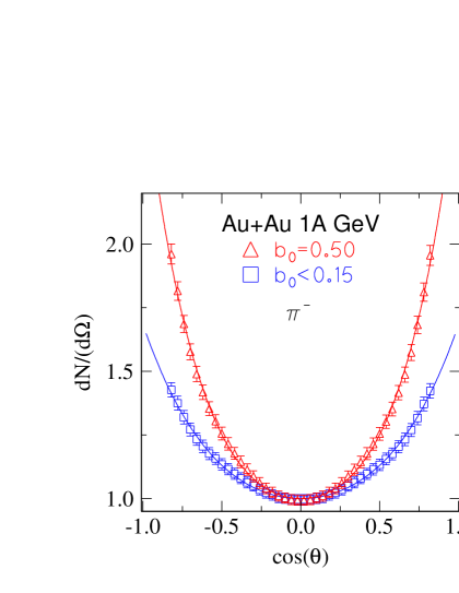
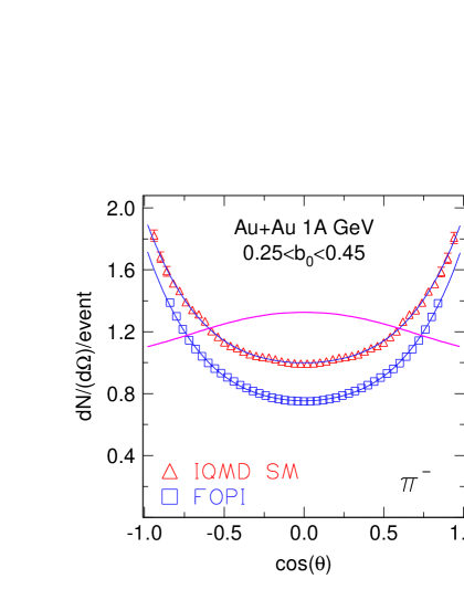
Figure 9: Polar (c.o.m.) angle distributions of $\pi^{-}$ mesons in the reaction Au+Au at $1A$ GeV. The solid lines are least squares fits of the three-parameter function $a_{0}+a_{2}\cos^{2}\theta+a_{4}\cos^{4}\theta$. Left panel: Experimental data. Open squares (blue): $b_{0}<0.15$, triangles (red): $b_{0}=0.50\pm 0.05$. The data have been normalized to 1 at $90^{\circ}$ to emphasize the differences in shape. Right panel: Comparison with IQMD for $0.25<b_{0}<.45$. The ratio IQMD/FOPI is also shown (Thick solid curve).

In terms of our $A_{f}$ the anisotropy measured [54] for central collisions ⁴⁰Ar + KCl at $1.8A$ GeV , $A_{f}=1.19$, compares well with our values of $1.21\pm 0.03$ and $1.22\pm 0.03$ for $6\%$ central collisions of ⁴⁰Ca + ⁴⁰Ca at 1.5 and $1.93A$ GeV, respectively.

The polar angle anisotropies cannot be explained in the framework of thermal models. The simulation with IQMD, however, does a reasonable job for this observable, aside from the absolute normalization to be discussed later (see right panel of Fig. 9). High polar angle anisotropies suggest that a significant fraction of the observed pions must be produced and emitted close to the system’s surface where they can escape without rescattering. One could conjecture that some, potentially more thermalized, pions (or nucleonic resonances) created deeper inside the system did not reach the detectors because of in-medium absorption.

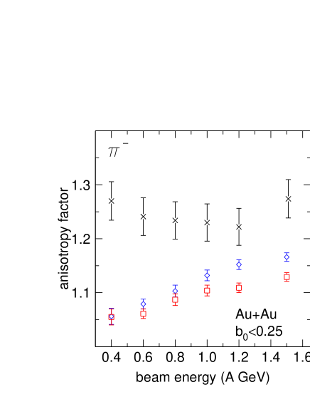
Figure 10: Excitation function of the anisotropy factor for Au+Au collisions with $b_{0}<0.25$. The (black) crosses are the measured data (with systematic errors), (blue) diamonds and (red) squares are predictions from IQMD SM and HM, respectively (with statistical errors).

More systematic details reveal differences between the data and the simulations. While stopping (Fig. 7) shows a weakly decreasing trend with increasing energy, the measured excitation function of $A_{f}$ looks rather flat (within the indicated systematic errors), see Fig. 10, while the IQMD simulations always underestimate $A_{f}$ and predict a rise with beam energy which is slightly more pronounced with the softer EOS.

The observables of anisotropy, $A_{f}$, and of stopping, $vartl$, are not equivalent since they quantify different aspects of momentum space population. However, they are related to the degree that high transparency that would yield $vartl\ll 1$ should be characterized by $A_{f}\gg 1$. The two branches seen in the stopping when varying either the size of the system or the geometry, Fig. 8, are also seen with the anisotropy observable, Fig. 11. IQMD simulations reproduce these features qualitatively. A somewhat puzzling feature is the fact that the measured data seem to suggest that the anisotropy grows slightly with $A_{part}$ when the centrality is kept high ($b_{0}<0.15$).

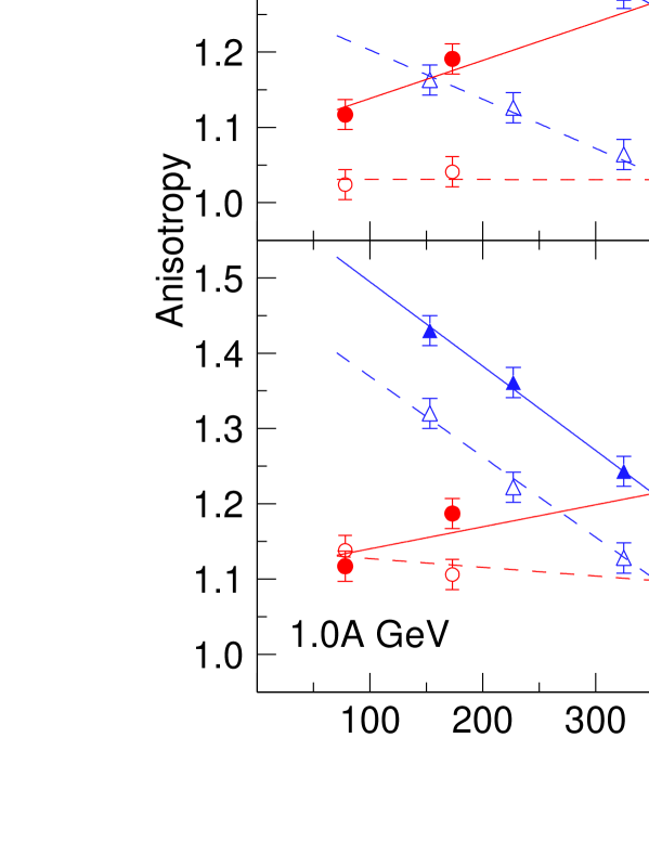
Figure 11: Anisotropy (averaged over $\pi^{-}$ and $\pi^{+}$) at 0.4, 1.0 and $1.5A$ GeV incident energy as a function of $A_{part}$. Full symbols and solid lines represent the data, open symbols and dashed lines represent the simulation IQMD SM. The lines are linear least squares fits added to guide the eye. As in Fig. 8, there are two branches, one varying $A_{part}$ via centrality $(b_{0})$ binning in Au+Au collisions, the other via changes of the system size $(A_{sys})$, keeping the centrality constant $(b_{0}<0.15)$.

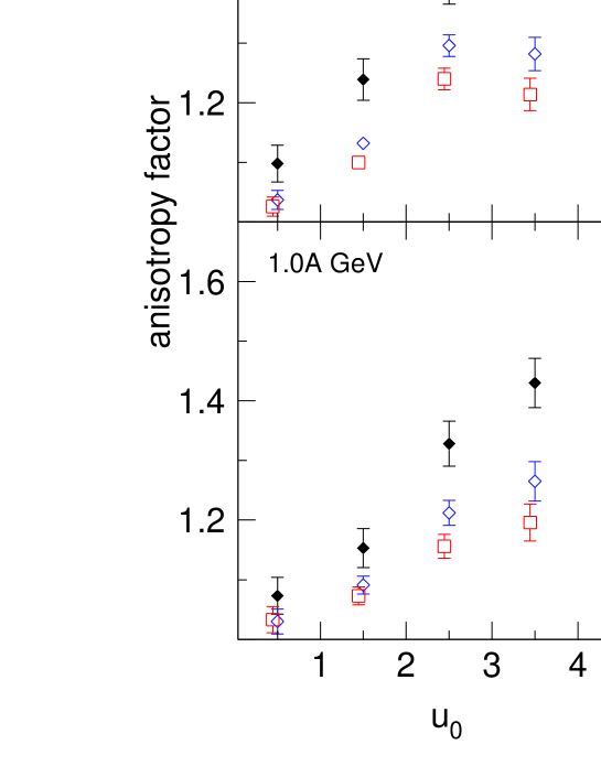
Figure 12: Anisotropy of $\pi^{-}$ in Au+Au collisions $(b_{0}<0.25)$ at 1.5, 1.0 and $0.6A$ GeV as a function of the scaled momentum $u_{0}$. Full (black) diamonds: data, open (blue) diamonds: IQMD SM, open (red) squares: IQMD HM.

In Fig. 12 we take a more differential look at anisotropy displaying for $b_{0}<0.25$ collisions the dependence on the scaled momentum $u_{0}\equiv(p/m_{\pi})_{0}$ ($m_{\pi}$ pion mass) for three different incident energies. The simulations with IQMD SM and HM are also shown. Again, IQMD underestimates $A_{f}$ systematically, shows a weak mean-field sensitivity and some tendency to saturate around $u_{0}\geq 3$. Except maybe at $1.5A$ GeV, the data do not show such saturation: $A_{f}$ rises approximately linearly within the $u_{0}$ range shown and converges to zero at zero momentum. This is expected on general grounds and indicates some consistency in our extrapolation to low $p_{t}$ which affects primarily $A_{f}(u_{0})$ values below $u_{0}=1$.

For inclusive data it appears that the momentum (or kinetic energy $E_{kin}$) dependence of $A_{f}$ shows a maximum near $u_{0}=2.8$ (or $E_{kin}$=150 MeV at $E/A=0.8A$ GeV) as demonstrated in Fig. 13 which reproduces the early data of Nagamiya et al. [51] for Ar+KCl at $0.8A$ GeV. It is interesting to note that the authors concluded (in 1981) ’these features cannot be explained by any conventional theoretical model’. In the figure we have included a calculation with IQMD for a similar system-energy, Ca+Ca at $1A$ GeV, which is seen to reproduce fairly well the observed features. Inclusive data are generally more difficult to interprete in a definite way. Due to trigger biases used to enhance central collisions and minimize background reactions [20] the present data cannot be directly compared with inclusive data such as those shown in Fig. 13.

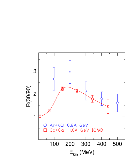
Figure 13: Ratio of pion yields at $30^{\circ}$ to that at $90^{\circ}$ for inclusive reactions. Circles: Ar+KCl at $0.8A$ GeV [51]. Squares joined by a smooth curve: Ca+Ca at $1A$ GeV using IQMD SM.

6 Pion production

6.1 Experimental trends

In this section we present our pion multiplicity data and compare the results with those of earlier work, as well as with those of transport model calculations.

In the earlier literature some authors reported on pion production in terms of pion multiplicity per ’participant’, $M(\pi)/A_{part}$. The motivation for this choice came from the observation, probably first reported in ref. [10], that in relativistic heavy ion reactions this reduced multiplicity did not appear to depend on the size of the system if the incident energy was kept fixed. Like impact parameters, ’participants’ (or ’spectators’) are not direct observables, they are not defined rigorously and are estimated using recipes that may vary with the authors. This limits the level of accuracy with which such ’reduced’ data from different experiments can be compared. In experiments that measure multiplicities eventwise there are two ways to determine the number of participants: first, one defines all nucleons to be participants that have momenta outside the Fermi spheres around target and projectile momenta, and, second, one calculates from the ’impact parameter’ the geometrical size of a straight-trajectory, sharp-geometry overlap zone [55] where the ’impact parameter’ is estimated from some global event observable ($ERAT$, charged particle multiplicity, etc) as described earlier. In the present work, using the second method and the observable $ERAT$, we estimate a $(90\pm 5\%)$ ’participation’ for our most central, $b_{0}<0.15$, sample.

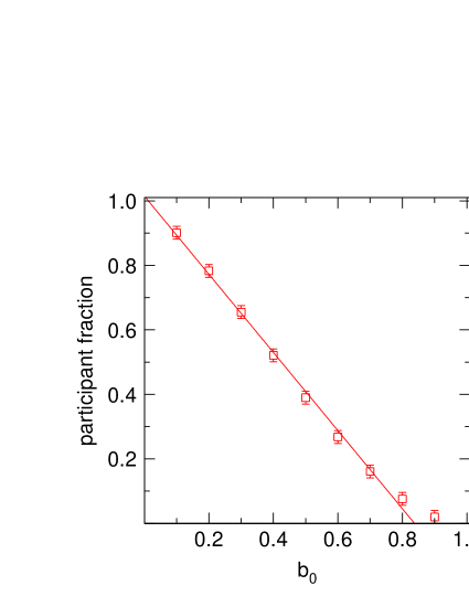
Figure 14: Dependence of the participant fraction on the scaled impact parameter $b_{0}$ in the sharp-cut geometrical model.

Although the calculation of $A_{part}$ with the sharp-cut geometrical model [55] is a simple mathematical exercise, we show the result in Fig. 14 to raise the awareness of an approximate fact: the participant fraction $A_{part}/A_{sys}$ decreases linearly with the reduced impact parameter $b_{0}$ if one confines oneself to $b_{0}<0.8$. Within this limit, it also does not matter much if the geometrical model allows for a diffuse [20], rather than a sharp surface.

For inclusive measurements, i.e. pion multiplicity data taken without a ’centrality bias’, $A_{part}=1/4A_{sys}$ is often assumed.

To our knowledge no single experimental apparatus measures all three isospin components of the pion. Assuming that Coulomb effects on pion production are very small, isospin symmetry implies that $M(\pi^{+})+M(\pi^{o})+M(\pi^{-})=3*M(\pi^{0})=1.5*[M(\pi^{+})+M(\pi^{-})]$. If only $M(\pi^{-})$ has been measured, assumptions must be made to obtain the full pion multiplicity, $M(\pi)=f*M(\pi^{-})$. Using for the following only the data for the most central collisions, our excitation functions for the total reduced pion multiplicity are simply excitation functions of the quantity $[M(\pi^{-})+M(\pi^{+})]*1.5/(0.9A_{sys})$.

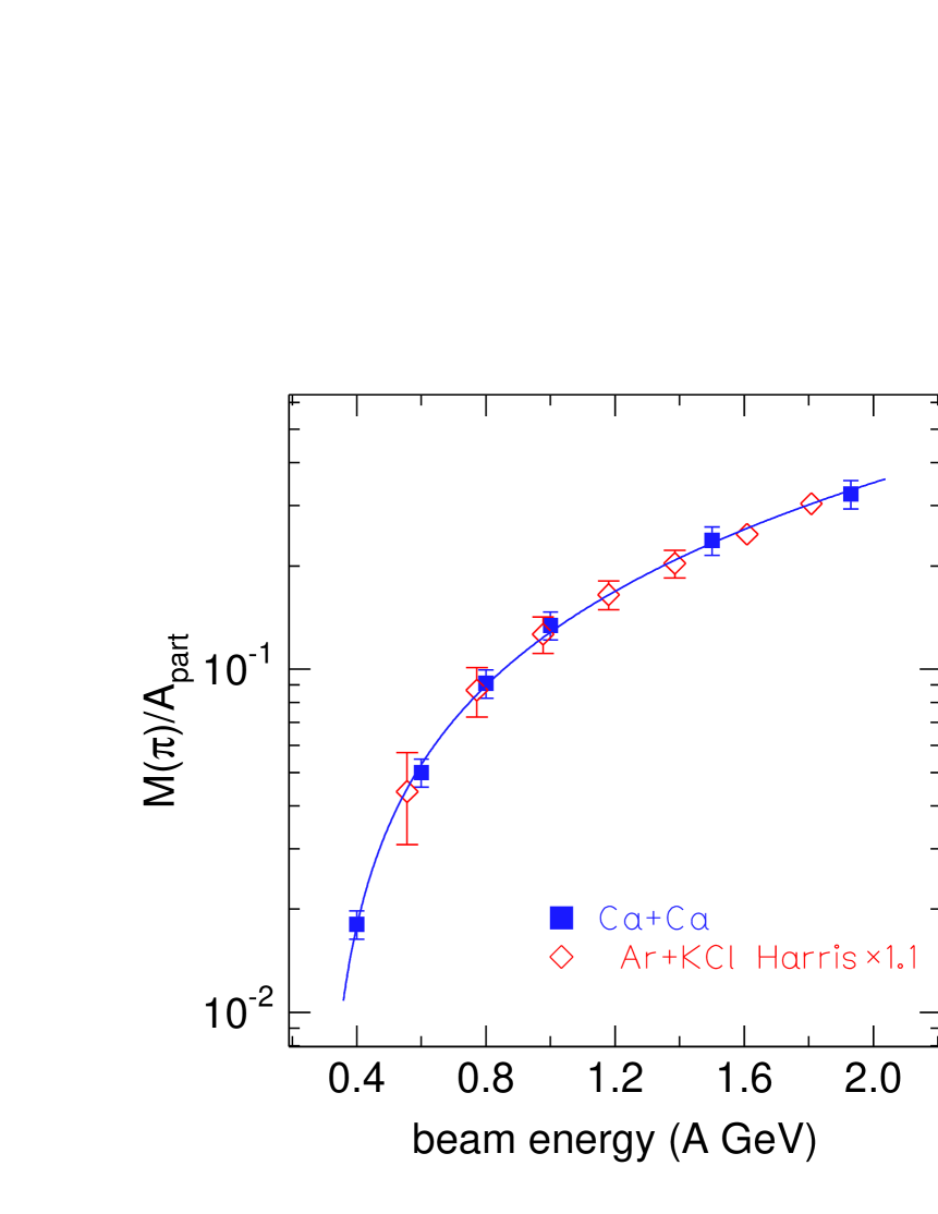
Figure 15: Excitation functions of the reduced pion multiplicity. The left panel compares the present data for Ca+Ca with the data (rescaled by a factor 1.1) of Harris et al. [12] for Ar+KCl. The right panel compares the present data for Au+Au with the La+La data [4].

The two-panel figure shows our measured pion-multiplicity excitation functions for the systems Ca+Ca (left panel) and Au+Au. They are compared with Streamer Chamber data for Ar+KCl [11, 56, 12] and for La+La [4], respectively. The smooth curve (a second order polynomial) has been fitted to the FOPI data only. The agreement between the two sets seems to be excellent.

At this point we have to remark that the present new Au on Au data are in conflict with our earlier publication [20] concerning pion production at $1.06A$ GeV. A reassessment of our older data has lead to the following conclusion: due to a too low setting of the potential voltage of the CDC the Chamber was not fully efficient for low ionizing particles (ref. [20] had reported the very first application of the CDC).

A few further comments on the comparison with the Streamer Chamber data are useful. In the La+La experiment [4] a 384 scintillator hodoscope covering angles $\theta_{lab}<18^{o}$ was added to the Streamer Chamber and the projectile-spectator angle window was defined ’to be the region centered about beam-velocity Z=1,2 fragments containing $90\%$ of the charged particles in minimum bias’. An efficiency factor, estimated from a cascade code simulation, was applied. The authors also mention a correction (approximately $14\%$) to the pion multiplicities to account for track losses and misidentifications. Finally, the negative pion multiplicities were multiplied by a factor f=2.35 to account for $\pi^{+}$ and $\pi^{0}$ emission. From our $\pi^{-}/\pi^{+}$ systematics we know that the factor depends on the incident energy (we estimate f=2.06 at .4A GeV and f=2.43 at 1.5A GeV for La on La).

Concerning Ar+KCl, the number of ’participating protons’ and the $\pi^{-}$ multiplicities are conveniently given in a Table [11]. Fragments with projectile velocity in a $4^{o}$ forward cone and positive tracks (around target rapidity) with laboratory momenta $p_{lab}<200$ MeV/c were counted as ’spectators’. All ’participant’ tracks were assumed to be singly charged. This is a good approximation at the highest energy. From the geometrical model we estimate a participant total charge of 28 (for a 180mb trigger) in reasonable agreement with the tabulated values [11] for beam energies above 1A GeV. The system Ar+KCl $(A_{sys}=77.25$, $Z_{sys}=36$ and hence $N_{sys}/Z_{sys}=1.146$) is not a strictly isospin-symmetric system. Using the simple-minded ’isobar’ formula [5] one obtains $M(\pi^{-})/M(\pi^{+})=1.255$, i.e. a number significantly different from 1 and implying f=2.70. Again, using our energy dependent systematics, we get factors f=2.55 at 0.4A GeV and f=2.74 at 1.5A GeV, rather than f=3 mentioned in [12]. From the tabulated ’proton participants’ and $M(\pi^{-})$ in [11] we get $M(\pi)/A_{part}$ values very close to those shown in [12] if we apply the isobar model f factor to the $\pi^{-}$ multiplicities and the factor $A_{sys}/Z_{sys}$ to the proton participant multiplicities. In our figure we show that we get perfect agreement with our data if we boost the Harris data by $10\%$. No correction for the Streamer Chamber response is mentioned in the three publications [11, 56, 12] which appear to pertain to the same experiment.

At the GSI/SIS accelerator site pion data have also been obtained using two other experimental setups. The pion multiplicity data of the TAPS collaboration have been summarized in [49]. Some (unpublished) data (for E/A=1GeV) from the thesis work of Wagner [57] measured with the KaoS setup, are listed in a Table of ref. [19].

A common feature of these experiments is that they are triggering on the particle(s) of interest (charged pions in the KaoS case and two-photon candidates for a $\pi^{0}$ decay in the TAPS case), within an angular range that is substantially limited if compared to the large acceptance devices (but can be varied by moving the apparatus). As a consequence they are not measuring pion multiplicities event by event, but rather differential cross sections in a restricted part of momentum space, preferably ’around mid-rapidity’, under more or less exclusive conditions. To convert the, apparatus-response corrected, data to reduced $4\pi$ pion multiplicities one must divide by a nuclear reaction cross section, $\sigma_{r}$ which in reference [49] was taken to be $\sigma_{r}=\pi r_{0}^{2}(A_{p}^{1/3}+A_{t}^{1/3})^{2}$ with $r_{0}=1.14$fm. Further, an extrapolation to phase-space outside mid-rapidity has to be made and possible biases in the triggering modes have to be corrected for if inclusive data are wanted. One asset of the TAPS method is that momenta are measured all the way down to zero. In Fig. 16 we compare the present Ca+Ca data and some of our earlier data [22], [23] with the inclusive TAPS data for neutral pions (multiplied by f=3) [49] for the systems Ar+Ca, Ca+Ca, recalling that the FOPI data are high centrality data. For completeness we also mention here TAPS data taken at much lower energies (Ar+Ca at $0.18A$ GeV [58]) well outside the range of the figure.

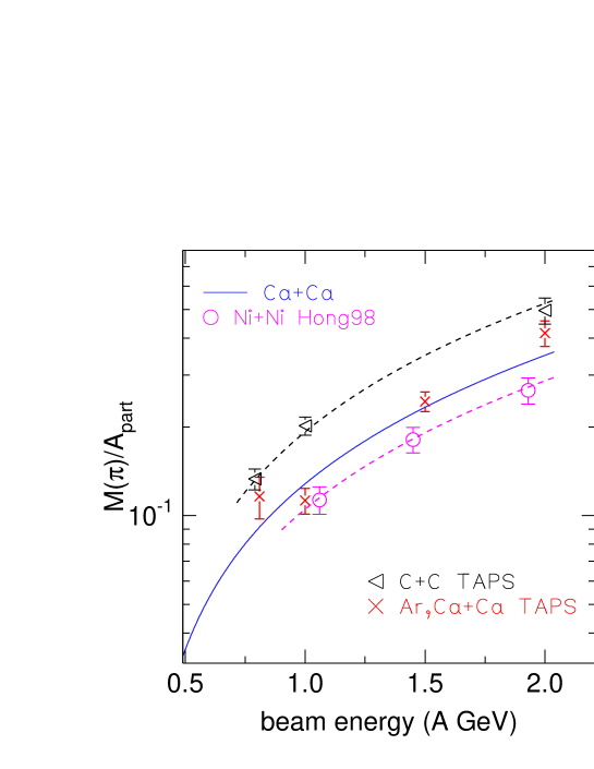
Figure 16: Excitation functions for the reduced pion multiplicities in reactions of Ca+Ca (smooth solid line identical to the one shown in Fig. 15), Ar+Ca and Ca+Ca [49], Ni+Ni [22], and C+C [49]. The respective symbols are indicated in the figure, for further comments see text.

The published mid-rapidity TAPS data have been obtained under the assumption of isotropic emission. Using our anisotropy information (previous section) we have boosted these data by a factor 1.25. If this is done, a satisfactory agreement with the FOPI data (and the old Streamer Chamber data) is obtained, the TAPS data having somewhat more straggling around the smooth trend inferred from our data (solid curve).

The figure also shows inclusive data for C+C, [59], again, corrected for anisotropy, and for central collisions of Ni+Ni [22, 23]. The two dashed curves represent the Ca+Ca curve (solid) rescaled by factors 0.82 and 1.58. Clearly, there is some system size dependence of the reduced pion multiplicity. We note that the C+C system corresponds to $A_{part}=6$ (inclusive data), the Ar+Ca (TAPS) data to $A_{part}=20$ and the FOPI data to $A_{part}=72$ and $100$ for Ca+Ca and Ni+Ni, respectively.

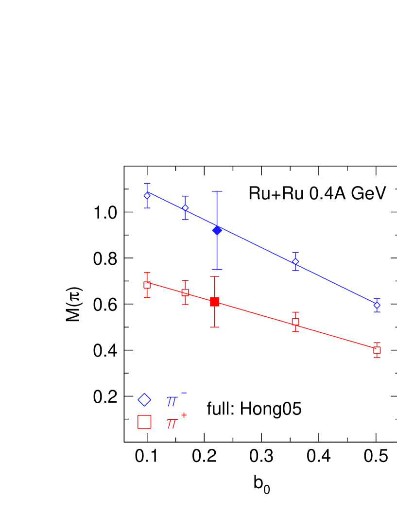
Figure 17: Multiplicities of $\pi^{+}$ and $\pi^{-}$ mesons in ⁹⁶Ru + ⁹⁶Ru reactions at $0.4A$ (left) and $1.5A$ GeV versus the reduced impact parameter $b_{0}$. The data points marked with larger full symbols are from an earlier publication [24].

Participant size dependences can also be shown by varying the collision geometry keeping the system fixed, as demonstrated in Fig. 17. The straight lines are linear least squares fits demonstrating (within error bars) the approximate linear dependence on the (reduced) impact parameter, which implies, as shown in Fig. 14, an approximate linearity also in terms of $A_{part}$. This figure also contains data from an earlier publication [24] of our Collaboration which used the alternate analysis method (’local tracking’) briefly described in subsection 3.

To obtain a quantitative evaluation of the $A_{part}$ dependence we confine ourselves first to the present data, thus avoiding systematic differences between various experiments and hopefully profiting from the smaller point-to-point errors. In the upper left panel of Fig. 18 we show the participant-size dependence of $M_{\pi}/A_{part}$ at an incident beam energy of 1A GeV.

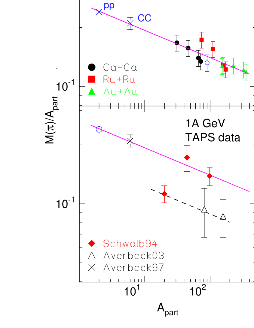
Figure 18: Reduced pion multiplicities and power law fits. The data points marked pp (or p) and CC (or C) are from refs. [60] and [59], respectively. The data in the left lower panel are TAPS data [59, 49, 61]. KaoS data [57, 19] are shown in the right lower panel. See text for further details.

It is of some interest to try to join up such data all the way down to the nucleon-nucleon system $A_{sys}=2$. This raises the question [19] how to define the number of ’participants’ in such a reaction. Specifically for the $pp$ reaction, we follow ref. [19] and use $(\sigma_{in}/\sigma_{tot})[M(\pi^{+})+M(\pi^{-})]*1.5/2$ where the multiplicities are obtained from the compilation (Table 4) of [60] and the ratio of inelastic to total cross section is set at 0.4 (for a 1A GeV incident beam). The resulting data point is marked $pp$ in the figure and plotted at $A_{part}=2$, simply because 2 is the minimum number of ’participants’ for any reaction. The second ’non-FOPI’ point, marked CC, has been determined by the TAPS collaboration [59] for inclusive reactions ($A_{part}=6$) and represents $1.25*3*M(\pi^{0})$, the factor 1.25 accounting conservatively for the (unknown) polar angle anisotropy, as discussed before. All other data are from the present work for various centralities plus a Ni+Ni point after [21] (for $A_{part}=90$, Fig.1). In the Figure the solid line is a power law fit, $M(\pi)/A_{part}=c*A_{par}t^{\tau-1}$, using only the FOPI data (i.e. $A_{part}>20$). We find $\tau=0.86\pm 0.04$, significantly different from one. (If it was one, the plotted reduced multiplicity would be constant.) This fit, somewhat surprisingly, is nicely compatible with both the $pp$ and the $CC$ data. Including all the data in the fit lowers the uncertainty of the $\tau$ parameter by a factor 2.

The power law curve is shown again in the other three panels. In the upper right panel of Fig. 18 we show only the data points for the most central collisions (except for the $pp$ and $CC$ data). The power law fit made to the more extensive set of data in the upper left panel is also optimal for this more limited set of data. The advantage of a limitation to very central collisions is that one is less dependent on the definition of $A_{part}$ since $A_{part}\approx A_{sys}$. At the higher energy, $1.5A$ GeV, the same type of data, also shown in the figure, are again fully compatible with an $A^{\tau}$ dependence, although $\tau=0.90\pm 0.02$ is somewhat closer to a pure ’volume’ dependence. In deriving power law descriptions of system-size dependences one hopes to distinguish between ’volume’ and ’surface’ effects in a way reminiscent of mass formulae, although the relative accuracy of mass measurements is multifold better (and therefore the results more convincing). Fitting the data with $c_{v}A+c_{s}A^{2/3}$ instead of $cA^{\tau}$, i.e. again with a two-parameter Ansatz, one can describe the $1A$ GeV data equally well as shown in the figure (dashed curve). One finds $c_{v}=0.096\pm.011$ and $c_{s}=0.186\pm 0.033$. With this description one can tentatively interprete the size dependence in terms of a decreasing surface to volume ratio: the fitted coefficients suggest a $52\%$ surface effect for C+C decreasing to $21\%$ for Au+Au (both for $b_{0}<0.15$ collisions).

In principle, one could also add an isospin term, again following mass formulae. The only unambiguous information in our data comes from a comparison of ⁹⁶Ru + ⁹⁶Ru with ⁹⁶Zr + ⁹⁶Zr. However, for the total multiplicity of pions (adding both charges) we found no significant difference within errors.

From the smoothened trends described by the power law fits we can deduce that the reduced pion yields in the reaction Au+Au around $1A$ GeV are lower by a factor of about 0.85 with respect to the Ni+Ni system. In Fig. 2 and Table 3 of ref. [21] we had concluded that this factor was about 0.53. As mentioned earlier, the partially inadequate operation of the CDC in the experiment leading to the results published in ref. [20] forces us to retract this number and most of the quantitative aspects of the conclusions in this early publication.

The TAPS data for 1A GeV [61, 59, 49] are shown in the lower left panel together with the $pp$ point. We have applied a factor 1.25 to these mid-rapidity data to correct them for the polar anisotropies discussed earlier. The data from the earlier publication [61], (red) full diamonds, for the systems Ar+Ca, Kr+Zr and Au+Au, have been later revised [49], black open triangles, to account for a trigger ’bias towards centrality’. However, the Ar+Ca point was not changed. These data were obtained in coincidence with the Forward Wall of FOPI. The C+C point was obtained in a different setup not involving the FOPI apparatus. As can be seen from the figure, after the revisal, the three TAPS points (triangles) appear to be aligned, but are significantly below the solid power law line (the dashed curve is our power law curve down-scaled by a factor 1.58). Note also that if the correction is due to a centrality bias the revisal also leads to a shift along the $A_{part}$ axis. Trying to join up the three revised points to the $CC$ and $pp$ data, one has to introduce two kinks in the overall TAPS curve.

Pion multiplicity data from the KaoS Collaboration are cited in [19] and taken from an unpublished part of the thesis work of Wagner [57]. The two data points for 1A GeV incident beams, cited as being inclusive, for Ni+Ni, resp. Au+Au, are shown in the lower left panel as taken from Table 2 of ref. [19]. Also shown in the right lower panel of Fig. 18 is a reassessment of these data points: first, a reaction cross section in line with our geometrical scaling ($r_{0}=1.15$) and the TAPS procedure ($r_{0}=1.14$) and, second, the application, again, of the anisotropy factor $A_{f}=1.25$. When this is done, the Ni+Ni point completely, and the Au+Au point marginally, agree with our power law fit.

It is of some interest to mention here that $\pi$-nucleus reaction data from the meson factories [1] have also been described in terms of power laws. In particular, ’true’ absorption [62] is characterized by $\tau=0.75\pm 0.05$ for (200-400) MeV/c pion momenta. However, the initial states of the ’inverse’ (absorption) reaction cannot be compared simply with the final states in the heavy ion induced pion emission. Indeed, in the latter case, a ’bulk’ or volume term for a strongly interacting particle like the pion (or its parent $\Delta$ baryon) can only be understood if one invokes a collective expansion mechanism allowing pion absorption to stop or ’freeze out’ globally at some time in the evolution of the reaction. This mechanism, presumably, is absent in $\pi$-nucleus reactions.

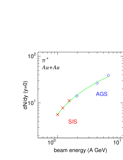
Figure 19: Excitation function for mid-rapidity $\pi^{+}$ mesons in central Au+Au collisions. The three data points at the higher energy are from ref. [63]. The data are for a centrality of $5\%$ (in terms of the reaction cross section) within a rapidity interval $|y_{0}|<0.25$.

The data of our present work for central Au+Au reactions join up smoothly to AGS data [63] if taken under the same exclusive conditions. This is shown in Fig. 19 for $\pi^{+}$ mid-rapidity data. Included in the figure is a least squares fitted second order polynomial, in terms of $\ln(E/A)$, that reproduces the six data points with an average accuracy of $6\%$, close to the point-to-point systematic errors of both collaborations. We conclude that there is no significant ’kink’ in this excitation function, as one might have expected to observe if the gradual passage to ’resonance’ matter (i.e. with a significant degree of nucleonic excitations) were to be associated with a fast increase of entropy.

6.2 Comparison with transport models

The old Ar+KCl and La+La data obtained at the BEVALAC accelerator with a Streamer Chamber [12, 4] seemed to indicate within error bars that the multiplicity per participant was independent on the size of the fireball at a fixed incident energy. The authors [4] concluded that ’pion production is a bulk nuclear-matter probe rather than a surface probe’ and ’is unaffected by the expansion phase’. As a consequence they deduced by comparison with thermal model expectations that the nuclear EOS (’missing energy’) ’is extremely stiff’. Probably the first publication putting into question the sensitivity of pion multiplicities to the EOS was ref. [6] in which a transport code based on the Boltzmann equation and including the mean field and Pauli blocking effects was used. Later, Kruse et al. [7] using a different code confirmed that they could not determine the EOS from the data of Harris et al. [12, 4], since they found only a $10\%$ effect when changing from a stiff to a soft EOS. In 1986 Kitazoe et al. [8] reported that they were actually able to reproduce the Harris data ’without introducing the nuclear compression effect’.

Fig. 20 shows a comparison of $4\pi$ integrated pion multiplicities ($1.5*(\pi^{+}+\pi^{-})$) with the predictions of IQMD for central ($b^{(0)}<0.15$) Au on Au collisions. The ratio theory to experiment is found to be $1.22\pm 0.08$ for the soft EOS (SM), a number that holds independently of the tracker (LT or HT) used. The HM (stiff) version predicts at the highest energy ($1.5A$ GeV) a drop of pion multiplicities by about $10\%$ and even less at lower energies. Danielewicz [43] showed that the ’missing energy’ conjectured to be the compression energy was actually taken up by the collective (radial) flow energy generated during the expansion which has a high degree, but not perfect, adiabaticity (and undergoes the associated cooling and memory loss).

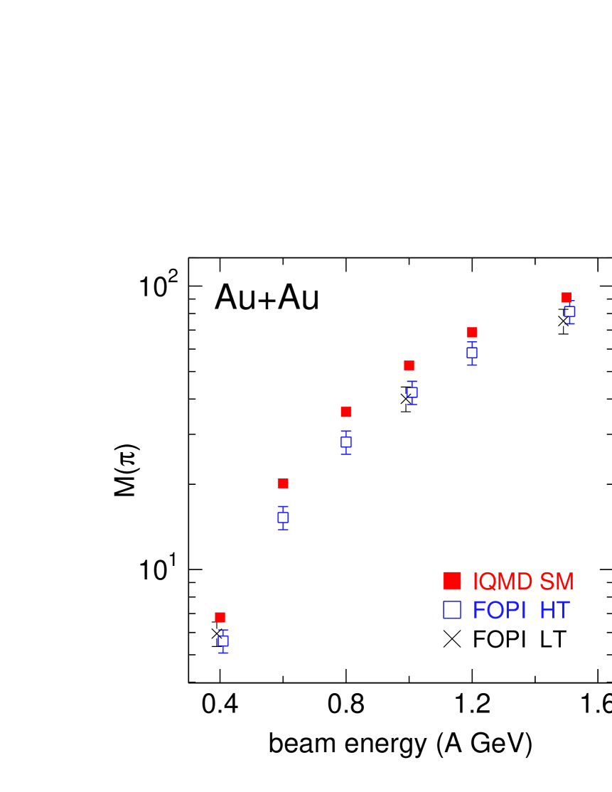
Figure 20: Left panel: excitation function for total pion multiplicity in central Au+Au collisions. For the data at 0.4, 1.0 and $1.5A$ GeV two different trackers have been used, HT and LT. The measured data are compared to a simulation using IQMD SM (full squares). Right panel: ratio theory/experiment (HT). Full squares: IQMD SM with the systematic uncertainties of the data; open triangles: IQMD HM.

In ref. [64] eight different transport codes were compared: the predictions for pion multiplicities in reactions of Au on Au at $1A$ GeV differed by a factor 1.6 if the ’standard’ versions were used. Some of this disturbing finding could be resolved by ’unifying’ the treatment of the $\Delta$ baryon lifetime in the medium which was found to strongly influence pion production. Performing an IQMD simulation with a ’phase shift prescription’ [65, 66, 64] instead of the prescription proposed in ref. [8], we found that the pion multiplicities for central Au+Au collisions were reduced by $(26-30)\%$ to values somewhat lower than the experimental values. As we shall see later, the phase shift prescription also influences the predicted pion flow, although not quite as significantly.

In ref. [42] a realistic estimation of in-medium modifications was performed. Perhaps the most spectacular and interesting effect originates from a significant modification of the ’elementary’ free cross sections for the $NN\rightarrow N\Delta$ reaction caused by the drop of the baryonic Dirac masses in the medium predicted presently by a number of theoretical models (see for example [67]). Within the quasiparticle picture this affects the kinematical phase space factors in front of the square of the transition matrix element determining the cross sections. Although, due to partial thermalisation and hence a setting in of the back reaction via detailed balance, this does not translate linearly to the observed pion multiplicities. The effects predicted [42] are still significantly larger than the experimental uncertainties.

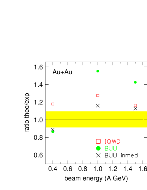
Figure 21: Ratio of theoretical and experimental pion multiplicities for central Au on Au collisions versus beam energy. Crosses and full circles are calculations from ref. [42] with and without in-medium corrected cross sections, respectively. The open squares are IQMD calculations with free cross sections. The shaded band reflects the uncertainty of the experimental data.

Medium effects are of special interest in this context since $\Delta$ baryon resonances decay in the medium due to their very short lifetime and undergo a cycle of several regenerations [33]. At present it seems that the theoretical situation regarding these matters is not settled. This is illustrated in Fig. 21 where we plot the ratio of calculated pion multiplicities to experimental data for Au on Au at various incident energies. The ratios were evaluated using BUU results from ref. [42] for the so-called NL2-set2 combination of parameters (see the original paper for details) which seemed to come closest to a preliminary version of our data. Compared to the experimental uncertainty band indicated in the figure the difference between the calculation fully accounting for in-medium modifications and the ’standard’ calculation with free cross sections is significant at the two higher beam energies. For comparison we also plotted the ’standard’ (in the present work) IQMD predictions. The standard versions of IQMD and BUU make different predictions. At $1.5A$ GeV the standard IQMD value is close to the in-medium corrected value of the BUU code.

7 Transverse momentum spectra

The main characteristics of pion emission transverse to the beam axis have been described in section 4 in terms of the variance of the transverse rapidity distribution which was compared with the variance of the longitudinal distribution. In this section we briefly compare transverse momentum spectra in more detail with, first, data from the KaoS Collaboration [68] and, second, with the output of IQMD calculations.

7.1 Comparison with KaoS

To convince ourselves that the filtered part of our data (upper right panel in Fig. 1) that we choose to analyse is not affected by $p_{t}$ dependent distortions in the $p_{t}$ range that we are interested in (i.e. excluding both very low $p_{t}$ which we cannot measure, as well as very high $p_{t}$ which are rare), we have made a comparison with KaoS data [68] for the reaction Au+Au at $1.5A$ GeV which is shown in Fig. 22. Notice the comparison is shown on a linear ordinate scale. To avoid the influence of assumptions and possible problems of aligning the centralities, we have chosen a relatively large sample (the 1200mb innermost centrality) at fixed laboratory angles indicated in the figure. The agreement is good as far as the shape of the spectra is concerned (the KaoS data have been rescaled to agree with the FOPI data on an integral basis). Below 0.1 GeV/c the FOPI data are affected by apparatus response.

7.2 Comparison with IQMD

Attempts to describe transverse momentum spectra in terms of thermal model parameters are generally successful, see for instance [22, 23, 24]. Here we shall not go through the thermal exercise, but are rather interested how well microscopic calculations that are free of ad hoc adjustable parameters are reproducing our data. In Fig. 7 we have shown that the variances of the transverse rapidities were rather well reproduced in Au+Au collisions. We normalize the calculations to the experimental data, since we have already discussed (see Fig. 20) the integrated pion multiplicities and are now interested in the shapes of the spectra. The outcome of the comparison is shown in Fig. 23 for the reaction Au+Au at $1.5A$ GeV and $b_{0}<0.15$. The, somewhat different, shapes of both the $\pi^{+}$ and $\pi^{-}$ mesons are well reproduced in the $p_{t}$ range shown. The level of accuracy on which the comparison is meaningful in the figure is determined by the systematic errors in the data and corresponds approximately to the size of the symbols. We recall that IQMD takes into account the effect of the Coulomb fields on the pion trajectories, but does not include (yet) higher resonances which might influence the spectra at higher momenta. With this partial success in hand, we can go back to the details of the collision history that a microscopic code is able to furnish. Rather than being a spectrum resulting from the decay of resonances moving locally around with a single temperature, the model tells us [31] that the measured spectrum is a superposition of pions from various $\Delta$ baryon generations representing different stages of the collision with spectra varying in ’hardness’ as time proceeds. This is a key to memorize some effect of the early compression stage in contrast to a completely equilibrated freeze out scenario and is probably the reason why an, albeit small, effect of the mean field on both the yields and the stopping can be seen. As we shall find out later, the mean field effect also influences the small azimuthal anisotropies.

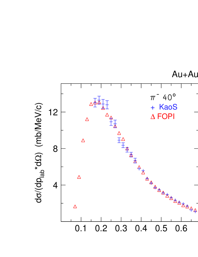
Figure 22: Laboratory momentum spectra, $d\sigma/(dp_{lab}d\Omega)$, of emitted pions at $40^{\circ}$ (left) and $60^{\circ}$ (right) for Au+Au at $1.5A$ GeV. The KaoS and the FOPI (triangles) spectra are compared for the same centrality selection.

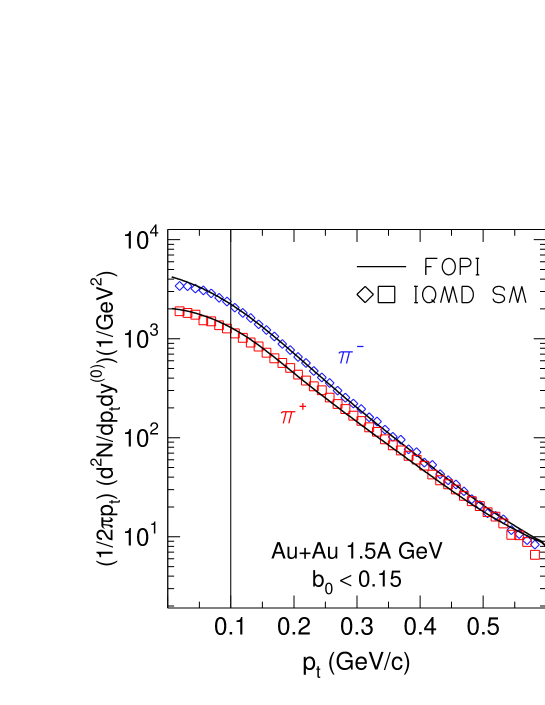
Figure 23: Transverse momentum spectra of $\pi^{-}$ and $\pi^{+}$ mesons in central collisions ($b_{0}<0.15$) of Au+Au at $1.5A$ GeV. The symbols represent IQMD simulations, the solid lines are generated from the smoothened representation of the measured data. The part to the left of the line at $p_{t}=0.1$ GeV/c is extrapolated. The spectra are integrated over the longitudinal rapidity $|y_{0}|<1.8$.

8 Pion isospin dependences

The $\pi^{-}$ and the $\pi^{+}$ mesons are members of an isospin triplet. A comparison of observables connected with differences between the $\pi^{-}$ and the $\pi^{+}$ mesons offers therefore, in principle, the possibility to explore isospin effects on the reaction dynamics and perhaps also on the more fundamental issue, the isospin dependence of the EOS.

In this section we show our results for the ratio of average transverse momenta and the ratio of yields. Another important observable, isospin differences in the pion flow, will be treated separately in section 9.

8.1 Average transverse momenta

In the simulation with IQMD, pions are assumed to propagate in Coulomb fields. As these change sign with the charge of the meson, higher average transverse momenta, $<p_{t}>$, are predicted for $\pi^{+}$ relative to $\pi^{-}$ mesons. This is shown in Fig. 24 for central collisions of the systems ⁴⁰Ca+⁴⁰Ca, ⁹⁶Ru+⁹⁶Ru, and Au+Au as a function of beam energy. The calculations predict an increase of the ratio $<p_{t}>^{+}/<p_{t}>^{-}$ with the total charge of the system, as one would expect, and an approximately linear decrease with the beam energy. The experimental data follow these trends, confirming, for this observable, the dominant influence of Coulomb fields, presumably after the strong interactions have frozen out. In principle this effect can be used to infer the size of the freeze-out volume. For an application of this idea using analytical formulae we refer to [69, 24]. Alternatively, since the microscopic simulation describes the transverse momentum data well, one could derive the freeze out conditions from the detailed intermediate output of the code. Here we rather invert the argument and conclude that the code is realistic as far as freeze out densities are concerned.

A closer look into Fig. 24 suggests that the decrease with beam energy is somewhat faster at the lower energy end and has a tendency to saturate at the higher energies. This effect is marginal however, in view of the experimental uncertainties, which are primarily caused by the necessity to extrapolate the measured data to zero $p_{t}$.

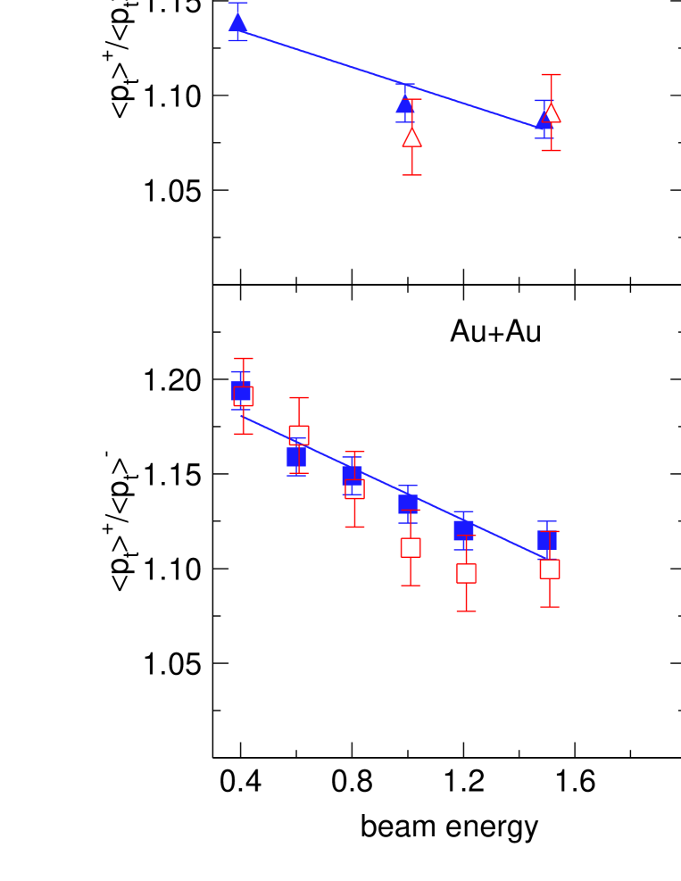
Figure 24: Ratio of the average transverse momenta of $\pi^{+}$ and $\pi^{-}$ mesons. Shown are the excitation functions for the systems Ru+Ru (top panel), Au+Au and Ca+Ca (lower right). The IQMD SM predictions (full symbols) are joined by linear least squares fits to guide the eye, the open symbols represent values inferred from our $4\pi$ extrapolated data.

8.2 Ratio $\pi^{-}/\pi^{+}$

The usefulness of the $\pi^{-}/\pi^{+}$ yield ratio for investigating the isospin dependence of the EOS has been advocated recently [70, 71]. The lessons learned in connection with total pion multiplicities (see section 6) leave room only for a cautious optimism.

It is argued [70] that both extremes of modelling, first chance collisions dominated by the $\Delta$-resonance mechanism (the $\pi^{-}/\pi^{+}$ ratio is then $\approx(N/Z)^{2}$ [5]), as well as equilibrium statistical models, via the difference $\mu_{n}-\mu_{p}$ in the neutron and proton chemical potentials, all depend on the isospin asymmetry densities quantified by $\rho_{n}/\rho_{p}$ or $\rho_{n}-\rho_{p}$ ($\rho_{n}$, $\rho_{p}$ are the neutron, resp. proton densities). Under the influence of the heavy ion dynamics changes in local asymmetries may be induced that in turn create different $\pi^{-}/\pi^{+}$ generations. In particular, if the EOS is stiff against isospin asymmetry at high densities, the local energy density will tend to minimize by pushing the neutrons out of high density areas (in neutron rich systems) leading to a local lowering of the $\pi^{-}$ production mechanism.

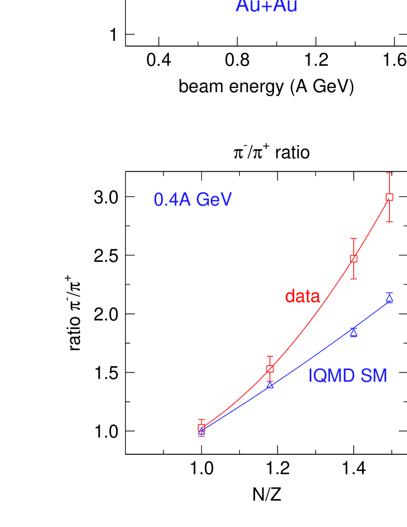
Figure 25: Upper left panel: Excitation function of the $4\pi$-integrated ratio of $\pi^{-}/\pi^{+}$ yields in central Au+Au collisions. The experimental data are joined by a least squares fit of the function $c_{0}+c_{-1}(E/A)^{-1}$ excluding the lowest energy point. The IQMD SM prediction (triangles) is also given. Upper right and lower left panels: the $N/Z$ dependence at $1.5A$, respectively $0.4A$ GeV of the $\pi^{-}/\pi^{+}$ ratio. The solid lines are least squares fits of linear or quadratic $(N/Z)$ dependence. Lower right panel: same as lower left panel,but for filtered data.

In the various panels of Fig. 25 we show a summary of our measured $\pi^{-}/\pi^{+}$ ratios and compare with IQMD predictions. Briefly, one observes a decrease of the $\pi^{-}/\pi^{+}$ ratio with incident energy (upper left panel) which is qualitatively also predicted by IQMD. However, in this panel, and more so in the other three panels, it is seen that while IQMD is doing a perfect job at $1.5A$ GeV, also when $(N/Z)$ is varied, it clearly underestimates the pion ratio for large $(N/Z)$ at $0.4A$ GeV. The right lower panel repeats the comparison at $0.4A$ GeV, but for the filtered data, leading to the same conclusion and thus showing that the extrapolations to $4\pi$ are not responsible for the discrepancy.

The linear $(N/Z)$ dependence at the higher energy instead of the expected $(N/Z)^{2}$ dependence of the $\Delta$-resonance model (the model used in IQMD) can be partially understood when realizing that the copious pion production will move the system towards chemical equilibrium by lowering the $(N/Z)$ of the daughter system constrained by total charge conservation [72]. However, the linear behaviour of IQMD at $0.4A$ GeV, where pion emission is a modest perturbation, is less trivial, all the more as it disagrees with the non-linear behaviour of the data.

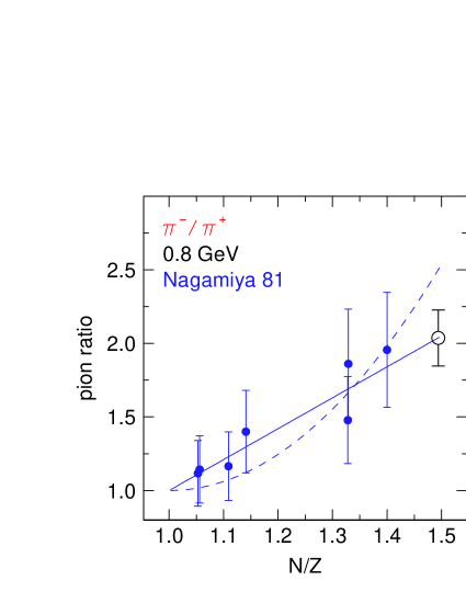
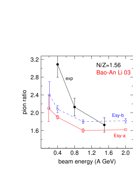
Figure 26: Left panel: $\pi^{-}/\pi^{+}$ ratio versus $N/Z$ of the ’fireball’ measured [51] in various inclusive heavy ion reactions at $0.8A$ GeV (full circles). The solid (dashed) curve is a linear (quadratic) least squares fit to the data constrained to be one at $N/Z=1$. The data point (open circle) from the present work holds for Au+Au and was not included in the fit. Right panel: $\pi^{-}/\pi^{+}$ ratios versus beam energy obtained in transport calculations [70] for the system ¹³²Sn+¹²⁴Sn ($N/Z=1.56$), using two options for the symmetry energy, Esy-b, dashed, and Esy-a. The ratios obtained from the present Au+Au data (solid circles) by linear extrapolation (from $N/Z=1.494$) are shown for comparison.

A systematics of $\pi^{-}/\pi^{+}$ ratios was first established for inclusive reactions [51] at $0.8A$ GeV beam energy using various, also asymmetric systems. In Fig. 26 we reproduce these older data which were plotted as a function of an estimated [51] ’fireball’ $(N/Z)$ composition. Due to the limited accuracy, both linear and quadratic $(N/Z)$ dependences are compatible with these inclusive data. Our data point for Au+Au at the same energy, but for a central collision selection, is also shown in the figure and is perfectly compatible with the linear extrapolation.

In ref. [70] Bao An Li has performed more advanced calculations for ¹³²Sn+¹²⁴Sn at $0.4A$ GeV using two different options for the asymmetry energy, Esy-a, a version that increases linearly with the density, and Esy-b, an exotic variant that after an increase at lower density bends back down to cross zero again at $\rho=3\rho_{0}$. The changes in the $\pi^{-}/\pi^{+}$ ratio that these very different alternatives induce are shown in Fig. 26 which reproduces results from Fig.2 of ref. [70].

The $N/Z$ ratio of the rare isotope beam combination, $N/Z=1.56$ is not very different from that of ²⁰⁸Pb+²⁰⁸Pb, $N/Z=1.536$ (which would be a more readily available bigger system). For the reaction ¹⁹⁷Au+¹⁹⁷Au studied here, $N/Z=1.494$, we anticipate, by linear extrapolation to $N/Z=1.56$, $\pi^{-}/\pi^{+}$ ratios that have been added to the figure. With this addition the problematics already known from the total pion multiplicity studies show up. First, the difference predicted from the calculation [70] between two rather extreme options is on the $10\%$ level and hence on the order of the present experimental accuracy, and, second, none of the two predictions follows the data. Similar conclusions follow if we take the calculations in ref. [71].

9 Azimuthal correlations (’flow’) of pions

Owing to collective flow phenomena, discovered experimentally in 1984 [73, 74], it is possible to reconstruct the reaction plane event-by-event and hence to study azimuthal correlations relative to that plane. We have used the transverse momentum method [75] including all particles identified outside the midrapidity interval $|y_{0}|<0.3$ and excluding identified pions to avoid autocorrelation effects.

We use the well established parameterization

$$u=(\gamma,\vec{\beta}\gamma)\ ;\ \ u_{t}=\beta_{t}\gamma$$

$$\frac{dN}{u_{t}du_{t}dyd\phi}=v_{0}[1+2v_{1}\cos(\phi)+2v_{2}\cos(2\phi)]$$

$$v_{0}=v_{0}(y,u_{t})\ ;\ \ v_{1}=v_{1}(y,u_{t})\ ;\ \ v_{2}=v_{2}(y,u_{t})$$

$$v_{1}=\left<\frac{p_{x}}{p_{t}}\right>=<cos(\phi)>\ ;\ \ v_{2}=\left<\left({\frac{p_{x}}{p_{t}}}\right)^{2}-{\left(\frac{p_{y}}{p_{t}}\right)}^{2}\right>=<cos(2\phi)>$$

where $\phi$ is the azimuth with respect to the reaction plane and where angle brackets indicate averaging over events (of a specific class). The Fourier expansion is truncated , so that only three parameters, $v_{0},v_{1}$ and $v_{2}$, are used to describe the ’third dimension’ for fixed intervals of rapidity and transverse momentum. Due to finite-number fluctuations the apparent reaction plane determined experimentally does not coincide event-wise with the true reaction plane, causing an underestimation of the deduced coefficients $v_{1}$ and $v_{2}$ which, however, can be corrected by studying sub-events: we have used the method of Ollitrault [76] to achieve this. The finite resolution of the azimuth determination is also the prime reason why the measured higher Fourier components turn out to be rather small.

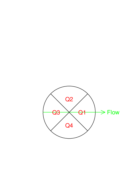
Figure 27: The four quadrants in a plane, $xy$, transverse to the beam direction, $z$. The flow direction, $x$, is indicated.

Alternatively to the three Fourier coefficients, one can introduce the yields $Q_{1}$, $Q_{2}$, $Q_{3}$, $Q_{4}$ in the four azimuthal quadrants, see Fig. 27, of which only three are independent (on the average over many events) due to symmetry requirements

$$Q_{2} = Q_{4}$$

$$Q_{0} = Q_{1}+Q_{2}+Q_{3}+Q_{4}$$

$$Q_{24} = Q_{2}+Q_{4}$$

The two equivalent triplets

$v_{0}$, $v_{1}$, $v_{2}$ $\longleftrightarrow$ $Q_{0}$, $Q_{1}$, $Q_{24}$

are related by

$$2\pi\ v_{0} =Q_{0}$$

$$\frac{2\sqrt{2}}{\pi}\ v_{1} =0.900v_{1} =\frac{Q_{1}-Q_{3}}{Q_{0}}$$

$$-\frac{2}{\pi}\ v_{2} =-0.637v_{2} =\frac{Q_{24}}{Q_{0}}-\frac{1}{2}$$

These relations show that $v_{1}$ is a dipole, while $v_{2}$ is a quadrupole strength. Statistical (count rate) errors can be deduced with use of elementary algebra. The quadrant formulation also has some advantage in assessing small apparatus distortions leading to systematic errors, as we shall see. The fact that $v_{1}$, as well as $v_{2}$, are found to be non-zero, is generally called ’flow’ in the literature and in particular the first Fourier coefficient is taken to be a measure of ’directed flow’, while the second Fourier coefficient has been dubbed ’elliptic flow’.

Recently more general methods based on Lee-Yang zeros have been proposed [77] and used [78] to isolate ’true’ collective flow from other effects that might influence azimuthal anisotropies. An analysis of some of our pion data with this method will be published elsewhere [78]. Here we take the point of view that the most likely ’non-flow’ correlation, the $\Delta$-correlation between nucleons and pions is part of the physics relating the pion flow to the nucleon flow, a physics that is implemented in the IQMD code that we use to try to understand the ’flow’ observables. Removing this correlation from the data would require removing it from the simulation as well when comparing. In view of the high statistics required to do this with sufficient accuracy we prefer in this survey to stick to the simpler ’standard’ method. This allows us also to compare with older data where possible.

Azimuthal anisotropies of pion emission in heavy ion reactions were first reported in the refereed literature by Gosset et al. [79] using the DIOGENE setup in the reaction Ne+Pb at $0.8A$ GeV. The authors attributed their observations to a target (Pb) shadowing effect. This study concerned primarily what is now termed the $v_{1}$ component. This $v_{1}$ component was studied in more detail in ref. [80] for the reaction of Au+Au at $1.15A$ GeV. The fact that in sufficiently non-central geometries the $\pi^{+}$ mesons had the opposite directed flow than the protons (termed ’antiflow’) was reported supporting earlier theoretical predictions [81, 33]. It was also observed that $\pi^{-}$ mesons had a different flow and it was concluded [80] that ’the differences between the behavior of the $\pi^{+}$ and the $\pi^{-}$ suggest that further consideration of this phenomenon is needed’.

The observation of a $v_{2}$ component was reported by the KaoS [82] and the TAPS [83] collaborations in 1993. A first shot at a $v_{2}$ systematics (Bi+Bi at 0.4, 0.7 and $1.5A$ GeV) was made in ref. [84]. A qualitative interpretation of the anisotropies making use of the transient vicinity of spectator matter close to the participant fireball as a ’clock’ was presented in ref. [85]. In terms of the azimuthal quadrants just introduced, the authors considered the ratios $Q_{1}/Q_{2}$, $Q_{3}/Q_{2}$ and $Q_{1}/Q_{3}$ which mix the two Fourier components $v_{1}$ and $v_{2}$.

A direct quantitative comparison of our present data and simulations with all these earlier observations is not straight-forward, as we shall see.

For completeness we mention here that pion flow has also been studied at much higher beam energies, $11A$ GeV (AGS [86]) and $40A$ GeV, as well as $158A$ GeV (SPS [87]). These incident energies are rather far apart, making it difficult to assess at present the gradual evolution of the pion flow observable and the associated physics changes.

As pion ’flow’ turns out to be small, when compared to nucleonic flow, its observation requires a high degree of systematic and statistical accuracy. Presently the latter is difficult to achieve in transport code simulations if one has the ambition to predict $v_{1}(y,u_{t})$ and $v_{2}(y,u_{t})$ in their full two-dimensional glory. Despite our computational efforts the simulations are still plagued with statistical errors that are a factor 3-5 larger than the experimental ones. Therefore, in the sequel we shall use several flow characterizers, $<v_{1}>$, $<v_{1}u_{t0}>\equiv<u_{x0}>$, $<v_{2}>$ and $<-v_{2}u_{t0}^{2}>\equiv<u_{yx}^{2}>\equiv<u_{y0}^{2}-u_{x0}^{2}>$ averaged ($<>$) over more or less large regions of phase space (besides the averaging over events of a specific centrality class). Although we present dipole and quadrupole flow in two separate subsections, they should be considered as two sides of the same (rather complex) phenomenon. In the sequel averaging brackets will be omitted, but will be implied.

9.1 Directed flow $v_{1}$

First, a few technical points will be mentioned. The near-equivalence of using the ’$\cos(\phi)$’ method, eq. , or alternatively the ’quadrant’ method, as well as the effect of the resolution correction are shown in Fig. 28.

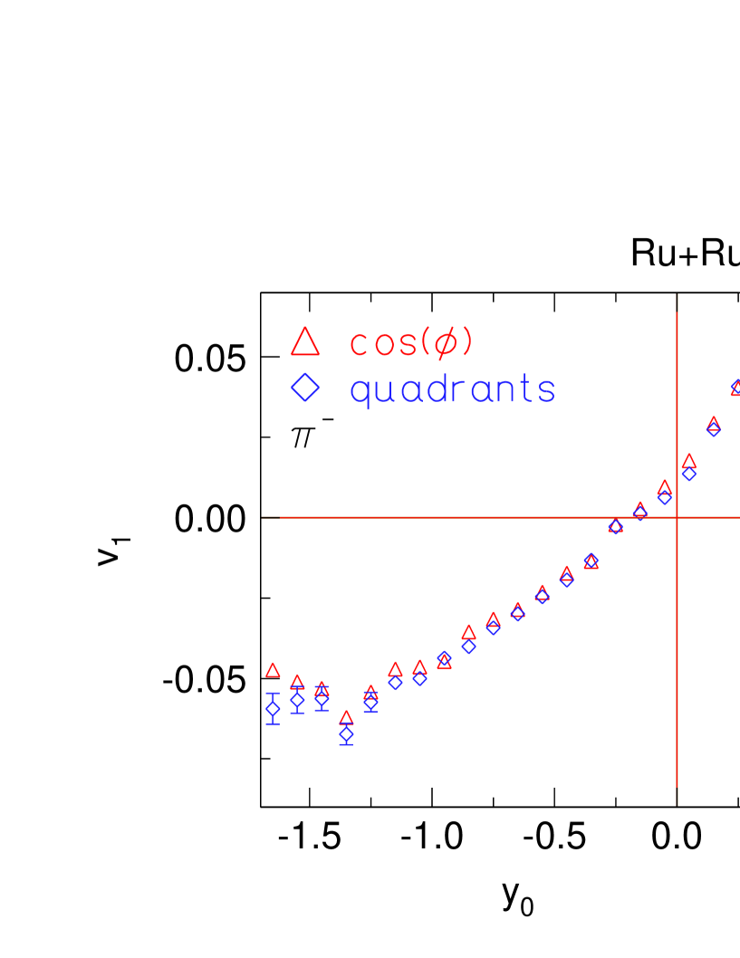
Figure 28: Rapidity dependence of the directed $\pi^{-}$ flow in the reaction ⁹⁶Ru + ⁹⁶Ru at $1.5A$ GeV. The centrality is $0.25<b_{0}<0.45$. Left panel: Comparison of the ’$\cos(\phi)$’ and the ’quadrants’ methods. Right panel: Comparison of the resolution corrected data with the uncorrected data.

Following [76] the correction factor is given by

$$v_{n}=v^{\prime}_{n}/<\cos(n\Delta\Phi)>$$

where $v^{\prime}_{n}$ is the (uncorrected) measured value and $\Delta\Phi=\Phi_{R}-\Phi_{R}^{\prime}$ is the azimuthal angle between the true and the measured reaction planes, $\Phi_{R}$ and $\Phi_{R}^{\prime}$, respectively. Due to the large acceptance of FOPI the correction factors are essentially given by the ’natural’ finite number fluctuations rather than by apparatus limitations. Typical values for different average centralities at an incident beam energy of $1A$ GeV are shown in Table 1. The effect of the correction is smallest when nucleonic flow is large, i.e. in the third centrality bin of the heaviest system. Small inhomogeneities in the laboratory azimuthal acceptances were found to have negligible influence on the flow results.

Table 1: Reaction plane resolution correction factors for $E/A=1A$ GeV.

$<b_{0}>$	Au+Au	Ru+Ru	Ca+Ca	Au+Au	Ru+Ru	Ca+Ca
		$\cos(\Delta\Phi)$			$\cos(2\Delta\Phi)$
0.100	0.852	0.707	0.561	0.583	0.365	0.216
0.167	0.910	0.786	0.609	0.708	0.471	0.259
0.360	0.963	0.892	0.698	0.860	0.663	0.353
0.502	0.958	0.894	0.699	0.845	0.670	0.354

————————————————————————-

For the symmetric systems that we study here, $v_{1}(y)$ should be asymmetric with respect to midrapidity ($y_{0}=0$), in particular $v_{1}(0)$ should be zero. As can be seen in Fig. 28, $v_{1}(y)$ does not cross the origin of the axes. A systematic study of this mid-rapidity offset showed that it depended on particle type, centrality and system size in a way suggesting that it was correlated with the track density difference in the ’flow’ quadrant $Q_{1}$ and the ’antiflow’ quadrant $Q_{3}$. While this could be simulated using our GEANT based implementation of the apparatus response, a sufficiently accurate quantitative reproduction of the offset at mid-rapidity was not achieved. We therefore opted for an empirical method to correct for the distortion, using the very sensitive requirement of antisymmetry with respect to midrapidity.

One can show that a good first order correction simply consists in shifting $v_{1}(y)$ down by a rapidity independent correction $\Delta v_{1}$ until it crosses zero exactly at mid-rapidity. Essentially $v_{1}\sim(Q_{1}-Q_{3})/Q_{0}$ ; assume we correct $Q_{1}$ by replacing it by $Q_{1}+cQ_{1}$ where $c$ is a constant not depending on transverse momentum or rapidity (some global loss in the flow quadrant). The correction to $v_{1}$ then is $\Delta v_{1}\sim cQ_{1}/Q_{0}\sim c/4$ where we use the approximation $Q_{1}\sim 1/4Q_{0}$. After trying different Ansatzes for the correction $c=c(y,u_{t})$ which could be in principle a 2-dimensional function, we ended up using the rapidity independent Ansatz $c=v_{0c}+v_{1c}*u_{t}$ which grows linearly with ut (or pt); $v_{0c}$ and$v_{1c}$ are parameters. The track density distortions are assumed to grow linearly with the density. The quadrant $Q_{3}$ is left unchanged (only relative corrections matter), $Q_{1}$ is replaced by $Q_{1}(1+c)$ and $Q_{24}$ by $Q_{24}*(1+0.55c)$ implying that in first approximation it is sufficient to use $Q_{2}\approx 0.55*(Q_{1}+Q_{3})$. Using the factor 0.55, ($\pm 0.05$), in the $Q_{24}$ correction, rather than 0.50, the value for isotropic emission, allows roughly for globally enhanced out-of-plane emission in the present energy regime. The values of $v_{0c}$ and $v_{1c}$ are fixed from the two mid-rapidity conditions $v_{1}(y_{0}=0)=0$ and $u_{x}(y_{0}=0)=0$. This is done separately for each particle,centrality and beam energy. The systematic error of $v_{1}$ after the distortion correction is assessed to be 0.007 or $7\%$ (whichever is larger) from the uncertainty of the mid-rapidity offset determination. The systematic error of $v_{2}$ (and $u^{2}_{yx})$) is $(7-10\%$) and was estimated by varying the coefficient for the $Q_{24}$ correction between 0.5 and 0.6. These systematic errors should be kept in mind when inspecting the figures presenting our flow data, as these contain only the statistical errors. In comparative cases, such as assessing isospin differences between the systems Zr+Zr and Ru+Ru the systematic errors are expected to cancel to some degree.

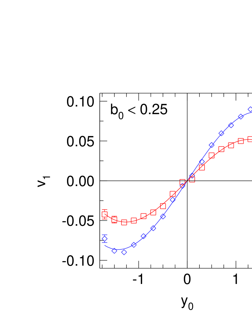
Figure 29: Rapidity dependence of the directed flow, $v_{1}(y_{0})$, for Au+Au collisions at $1.5A$ GeV with centralities $b_{0}<0.25$, $0.25<b_{0}<0.45$, $0.45<b_{0}<0.55$ (from left to right). The data are taken in the interval $1.0<u_{t0}<4.2$. (Red) squares: $\pi^{+}$, (blue) diamonds: $\pi^{-}$. The solid curves are least-squares fits, see text.

We are now in a position to review a representative sample of the rich flow data that we obtained in the present work. We start with the well known ’S-shaped’ curves for the rapidity dependence of flow, $v_{1}(y_{0})$. Fig. 29 shows the data for Au+Au at $1.5A$ GeV and for three of our ’standard’ centrality intervals. Several remarks can be made. Only the data for $y_{0}<0$ were actually measured, (anti)symmetry was used to infer the $y_{0}>0$ behaviour. As $b_{0}$ is increased, the diagrams ’rotate’ clockwise, the $\pi^{+}$ data always ’preceding’ the $\pi^{-}$ data. In the interval around $b_{0}=0.5$ this ’rotation’ has moved into a new ’quadrant’, the antiflow side, for the $\pi^{+}$. It is clear from this observation that pion flow cannot be simply derived from a ’parent’ $\Delta$ baryon flow assuming the latter to be equal to that of single protons, as was attempted in ref. [84] (for the elliptic part of the flow). A key question of theoretical analysis will be whether the $\pi^{+}/\pi^{-}$ difference (’isospin differential flow’) is just a Coulomb effect or rather necessitates a (nuclear) isospin effect in order to be reproduced.

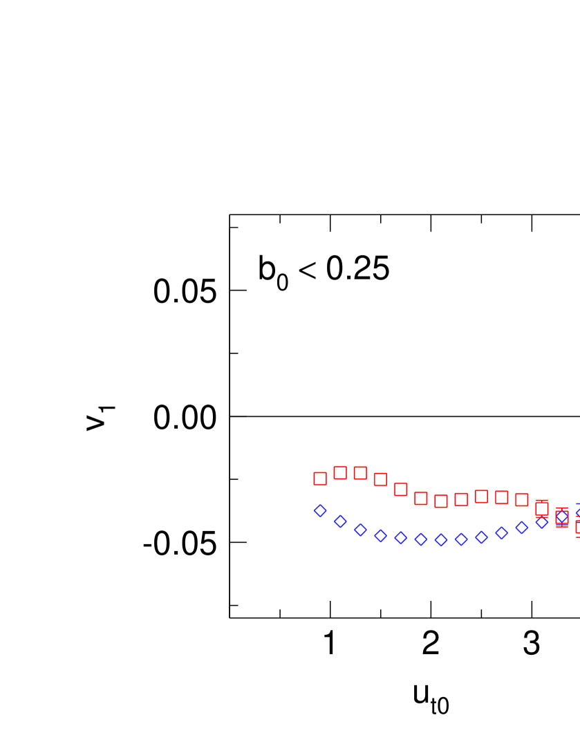
Figure 30: Transverse momentum dependence of the directed flow, $v_{1}(u_{t0})$, for Au+Au collisions at $1.5A$ GeV with centralities $b_{0}<0.25$, $0.25<b_{0}<0.45$, $0.45<b_{0}<0.55$ (from left to right). The data are taken in the rapidity bin $-1.8<y_{0}<0.0$. (Red) squares: $\pi^{+}$, (blue) diamonds: $\pi^{-}$.

In Fig. 30 we present the transverse momentum dependence, $v_{1}(u_{t0})$, for data integrated over the backward hemisphere. The switch of sign for $\pi^{+}$ near $b_{0}=0.5$ is again visible. There is a puzzling weak wavy aspect, especially in the $\pi^{+}$ data that is at the limit of apparatus distortions that we cannot completely exclude. However, a simulation with IQMD, not shown here, predicts qualitatively similar, even more pronounced, structures.

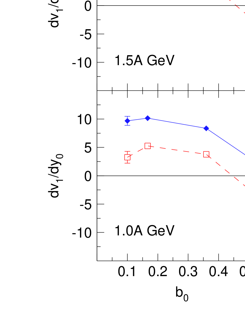
Figure 31: Centrality dependence of the midrapidity slope $dv_{1}/dy_{0}$ at various indicated beam energies in the reaction Au+Au. Open squares joined by dashed lines: $\pi^{+}$, full diamonds: $\pi^{-}$.

Although the detailed shapes of the flow data are seen to be complex, it is of some interest to try to characterize flow with just one parameter, thus easing the task of obtaining a survey of many system-energy-centralities. One such parameter, the midrapidity slope $dv_{1}(y_{0})/dy_{0}|_{y0=0}$, stresses more the midrapidity region, while the alternative parameter, which we term ’large acceptance’ flow is $v_{1}$ (or $u_{x0}$) averaged over a large region of momentum space and stresses more the regions closer to target (or projectile) rapidity since $v_{1}$ is zero at $y_{0}=0$.

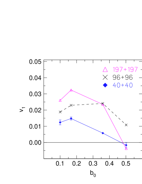
Figure 32: Centrality dependence of directed flow, $v_{1}$, for various indicated system masses and incident beam energy $1.5A$ GeV. The flow is averaged over $\pi^{+}$ and $\pi^{-}$. The values for $A_{p}+A_{t}=96+96$ are an average between Zr+Zr and Ru+Ru.

A survey of midrapidity slopes in Au+Au reactions as a function of centrality is shown for various indicated beam energies in Fig. 31. The slopes were determined by least squares fitting with the polynomial $v_{10}+v_{11}y_{0}+v_{13}y_{0}^{3}$ in the rapidity range $-1.8<y_{0}<0$ (the data are averaged over the interval $1<u_{to}<4.2$). The quality of the fits can be visualized in Fig. 29 (smooth curves). The constant $v_{10}$, which should be zero, accounts for remaining uncertainties of the offset correction described earlier, $v_{13}$ is necessary because, obviously, $v_{1}(y_{0})$ is not linear over the extended rapidity range and, finally, $v_{11}$ is identical to the slope $dv_{1}(y_{0})/dy_{0}$ at $y_{0}=0$. The $\pi^{+}$ slope data are seen to vary moderately with energy, the gap to the $\pi^{-}$ slopes widens at the lower energies.

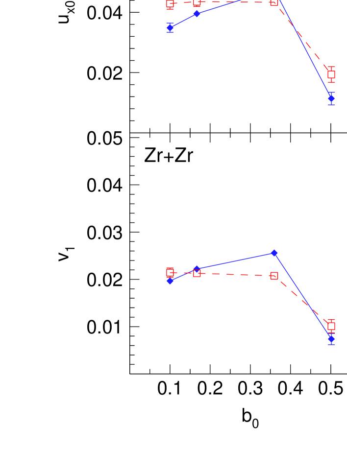
Figure 33: Comparison of the centrality dependence of directed flow ($v_{1}$ bottom and $u_{x0}$ top) in the systems ⁹⁶Zr+⁹⁶Zr (left) and ⁹⁶Ru+⁹⁶Ru (right). Open squares joined by dashed lines: $\pi^{+}$, full diamonds: $\pi^{-}$.

System size dependences and the system isospin dependences are shown in terms of the large acceptance flow in Figs. 32 and 33. For the averaging we choose the intervals $-1.8<y_{0}<0$ and $0.8<u_{t0}<4.2$ which are well covered by our setup for all measured system-energies. Although the data were obtained in the backward hemisphere we give the values in the forward hemisphere (which are opposite in sign) so that positive (negative) values mean ’flow’ (’antiflow’) analogue to the midrapidity slopes. For the size dependence study we have removed the isospin difference by averaging over $\pi^{-}$ and $\pi^{+}$ data and also, for mass $96+96$, by averaging over the two systems ⁹⁶Zr + ⁹⁶Zr and ⁹⁶Ru + ⁹⁶Ru. The system size dependence of directed flow is seen to be complex, in contrast to elliptic flow (see next subsection).

The last two mentioned systems were also the basis for an isospin dependence study, see Fig. 33. We find for $v_{1}$, as well as for $u_{x0}$ (both in large acceptance), an indication that the $\pi^{-}-\pi^{+}$ difference is slightly larger for Ru+Ru than for Zr+Zr. The Coulomb potential difference between the two systems is expected to be close to $10\%$, a difference that does not seem to account quantitatively for the observations. Since $N/Z$ is larger for the Zr+Zr system, this can only be understood if there is a nuclear isospin effect opposite in sign to the Coulomb effect. This seems to be also suggested by the theoretical investigations of Qingfeng Li et al. [44]. We shall come back to this when adding later also information on isospin differential elliptic flow (Fig. 40) which is easier to parameterize.

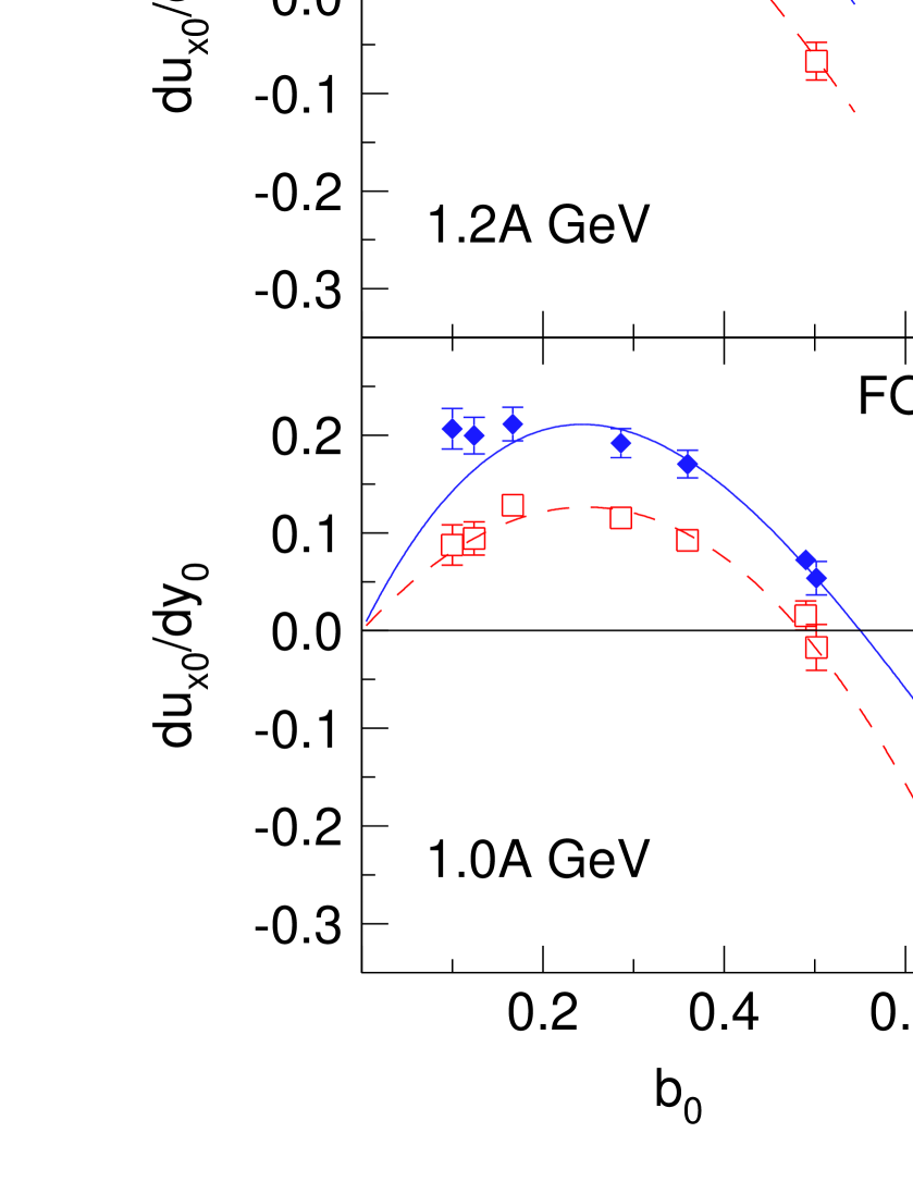
Figure 34: Centrality dependence of the midrapidity slope $du_{x0}/dy_{0}$ in the reaction Au+Au (squares and dashed lines: $\pi^{+}$, full diamonds: $\pi^{-}$). The left panels represent the data of the present work (’FOPI’) for $1.0A$ and $1.2A$ GeV beam energy with polynomial fits and a cut $1.0<u_{t0}<4.2$. The right panel is adapted from ref. [80] for $1.15A$ GeV.

Before trying to assess the sensitivities of pion flow data to theoretical input, we shall compare our data with those of ref. [80] which were taken at 1.15A GeV for the system Au+Au. Such comparisons are not trivial, as the system-energy, the centrality, the chosen specific flow-describing observable, and, last but not least, the phase space covered, must be ’aligned’. Fig. 34 presents in three panels the data relevant for this comparison in terms of the centrality $(b_{0})$ dependence of the mid-rapidity slope $du_{x0}/dy_{0}$. As we have no measurement at $1.15A$ GeV, we show in two of the panels our data at $1.0A$ and $1.2A$ GeV. The analysis of the $1A$ GeV data has been extended to higher $b_{0}$ to allow for a more complete comparison, but one can say that there is no dramatic difference between the two energies. The Kintner data have been converted to the same, scaled, axes using the information from Fig. 3 of ref. [80]. Similar to the slopes of $v_{1}(y_{0})$, our mid-rapidity slopes were determined from a least squares fit of $u_{x0}(y_{0})$ to the polynomial $u_{x00}+u_{x01}y_{0}+u_{x03}y_{0}^{3}$ in the backward hemisphere $-1.8<y_{0}<0$. At midrapidity $du_{x0}/dy_{0}=u_{x01}$, while the constants $u_{x00}$ and $u_{x03}$ take care of the uncertainty of the offset correction and of non-linearities in the rapidity dependence, respectively. The quality of these fits is generally excellent and similar to those shown in Fig. 29 for $v_{1}(y_{0})$.

Interpolating our data at $1A$ GeV, we find compatibility with the data of Kintner et al. at $b_{0}=0.6$, but for lower $b_{0}$ the evolution is different. The crossing point to ’antiflow’ of the earlier data is seen to occur roughly around $b_{0}=0.2$ for $\pi^{+}$, whereas our data suggest this to happen for $b_{0}=0.45-0.55$. This difference exceeds the uncertainty of the centrality determination in both experiments. For $\pi^{-}$ the data of ref. [80] are very close to the no-flow axis (given the error bars) preventing a reliable determination of the crossing point, which appears in our data to be shifted by about 0.1 units relative to the $\pi^{+}$ curve. Also, our data show more $\pi^{-}$ flow in the maximum near $b_{0}=0.25$. The midrapidity observable $du_{x0}/dy_{0}$ depends on the transverse momentum range covered: in our case sharp cuts were applied ($1.0<u_{t0}<4.2$, or $0.10<p_{t}<0.43$ GeV/c at $E/A=1A$ GeV). The low $p_{t}$ limitations of the data were not discussed in ref. [80].

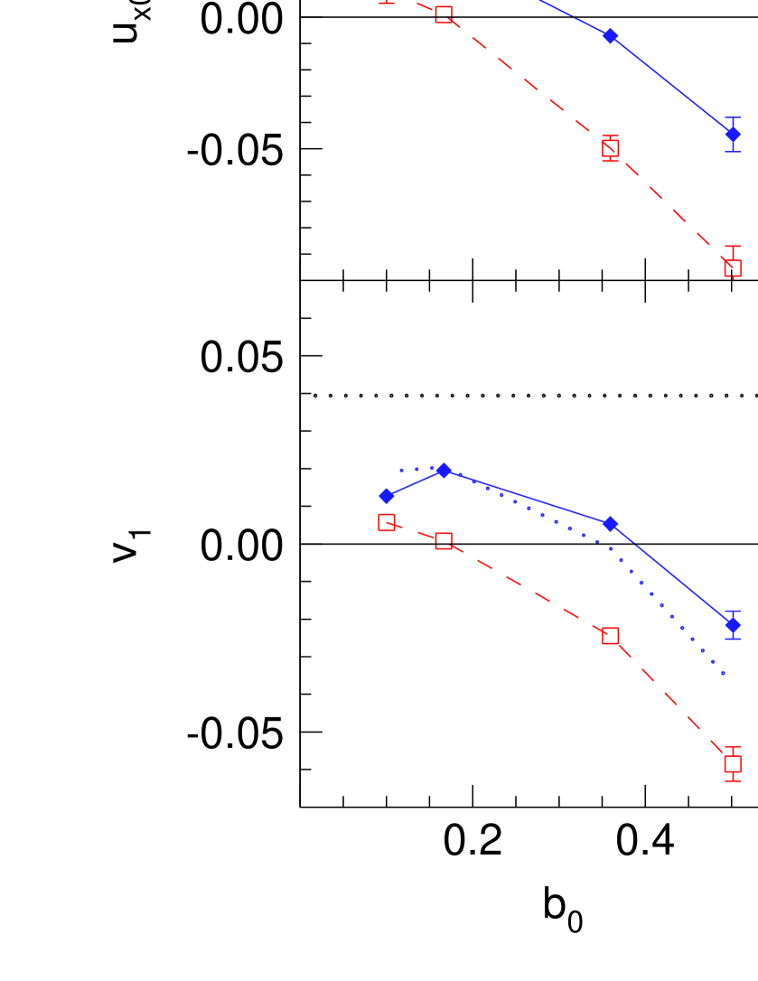
Figure 35: Centrality dependence of large acceptance (see text) directed flow in the reaction Au+Au at $1.5A$ GeV (squares and dashed lines: $\pi^{+}$, full diamonds: $\pi^{-}$). Going from left to right, the middle panels (’FOPI’) represent the measured data for $v_{1}$, $u_{x0}$ and the isospin differential flow $Du_{x0}$. The left (right) hand panels are the simulated data using a soft (stiff) equation of state. The dotted horizontal lines are merely references to guide the eye. The result of a linear least squares fit to the experimental isospin-differential flow (top middle row) is repeated in the adjacent upper panels. The dotted curve in the lower left panel results from a calculation (for $\pi^{-}$) with the phase shift prescription.

Moving now to a comparison with simulations, we have chosen the large acceptance flow, $|y_{0}|<1.8$ and $0.8<u_{t0}<4.2$, for this purpose as it requires less events for a given statistical accuracy. The comparison is presented in Fig. 35 for the reaction Au + Au at $1.5A$ GeV where the experimental data for $v_{1}(b_{0})$ and $u_{x0}(b_{0})$ and the isospin differential flow $Du_{x0}=u_{x0}(\pi^{-})-u_{x0}(\pi^{+})$ are framed by calculations with a soft EOS (left panel) and a stiff EOS (right panels). The stiff EOS predicts statistically significantly higher values of both $v_{1}$ and $u_{x0}$ and a transition to antiflow in more peripheral collisions. This sensitivity was noted earlier [9]. In the ’standard’ version of IQMD we use, the stiff EOS is closer to the data, especially for central ($b_{0}<0.2$) collisions. However, even the stiff EOS predicts a transition to antiflow at smaller $b_{0}$ than our data. This conclusion is not changed if we shift to the phase shift prescription for the $\Delta$ baryon lifetime although this option changed the pion multiplicities significantly (section 6.2). In the lower left panel of Fig. 35 we show also a calculation (dotted curve) with the phase shift prescription for $\pi^{-}$. The statistical errors (not shown) are similar to those of the standard calculation.

The systematic difference between $\pi^{-}$ and $\pi^{+}$ flow is reproduced and seems to be unaffected by the EOS. Since we have not used an isospin dependent EOS, any isospin effect in the calculation, besides Coulomb fields, would have to result from the ’cascade’ (i.e. collision) part of the model. Past experience has shown that cascade effects influence directed flow only moderately. The upper middle panel shows that $Du_{x0}(b_{0})$ varies linearly: the fit to the difference data is also plotted in the panels showing $Du_{x0}$ from the calculations. The calculated $Du_{0}$ are similar to to the experimental values but, despite the statistical limitations, seem to indicate a small surplus at intermediate $b_{0}$, possibly a consequence of the missing nuclear isospin mean field in the simulation. The effects are small and hence difficult to assess quantitatively in a convincing way.

9.2 Elliptic flow $v_{2}$

The presentation of our elliptic flow data follows in many ways the scheme of the previous subsection on directed flow. We start with aspects of rapidity and transverse momentum differential flow in the reaction Au+Au at $1.5A$ GeV, then switch to a systematics of beam energy, system size and system isospin dependences. Then we compare our data to earlier measurements where possible and finally compare a subset of the data to theoretical simulations.

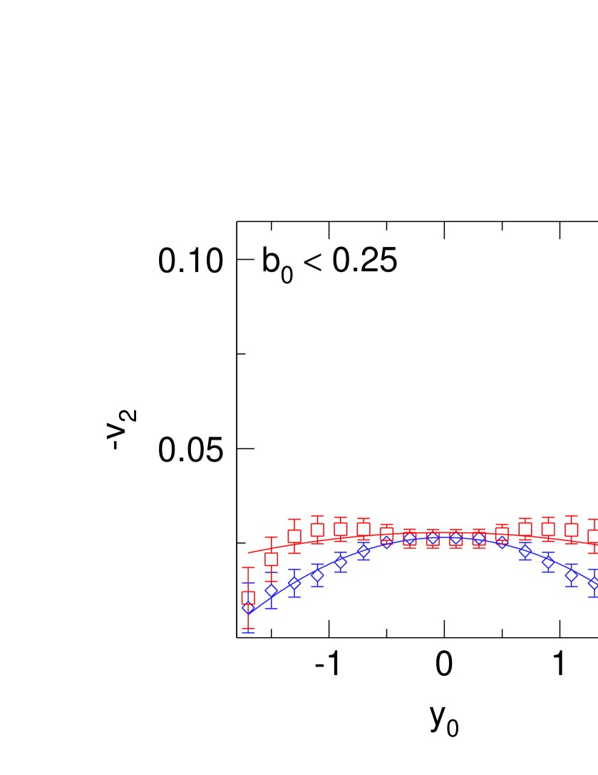
Figure 36: Rapidity dependence of the elliptic flow, $v_{2}(y_{0})$, for Au+Au collisions at $1.5A$ GeV with the indicated centralities. The data are taken in the interval $1.0<u_{t0}<4.2$. The solid curves are least squares fits of the two-parameter function $c_{0}+c_{2}y_{0}^{2}$. (Red) squares: $\pi^{+}$, (blue) diamonds: $\pi^{-}$.

In Fig. 36 we show the rapidity dependence of elliptic flow, $v_{2}(y_{0})$, for Au+Au collisions at 1.5A GeV for various centralities. Again, the flow of $\pi^{+}$ is different from that of the $\pi^{-}$, the difference increasing with impact parameter. The rapidity dependence is relatively flat: elliptic pion flow is not limited to a narrow mid-rapidity interval. There seem to be some weak structures (we remind however that only the backward hemisphere was covered by our analysis). These marginal structures can be evened out by the two-parameter polynomial fits (see the caption) on a level that is close to the statistical freedom and therefore will not be discussed further. The transverse momentum range is again sharply cut in the limits $1<u_{t0}<4.2$. Note that we always plot $(-v_{2})$, rather than $(+v_{2})$. The sign of $v_{2}$ tells us that there is a surplus of emitted pions in the direction ($y$) perpendicular to the reaction plane (zx).

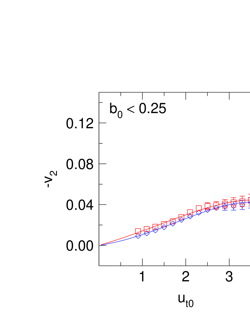
Figure 37: Transverse momentum dependence of the elliptic flow, $v_{2}(u_{t0})$, for Au+Au collisions with indicated centralities. The rapidity interval is $-1.8<y_{0}<0$. The solid curves are least squares fits of the polynomial $c_{1}u_{t0}+c_{2}u_{t0}^{2}+c_{4}u_{t0}^{4}$ to guide the eye. (Red) squares: $\pi^{+}$, (blue) diamonds: $\pi^{-}$.

The transverse momentum dependence of elliptic flow, $v_{2}(u_{t0})$, integrated over the backward hemisphere, is shown in Fig. 37. It rises with transverse momentum but seems to saturate beyond $u_{t0}=3$ (or $p_{t}=0.375$ GeV/c at $1.5A$ GeV). The difference between $\pi^{+}$ and $\pi^{-}$ flow is small but statistically significant for intermediate centralities and momenta.

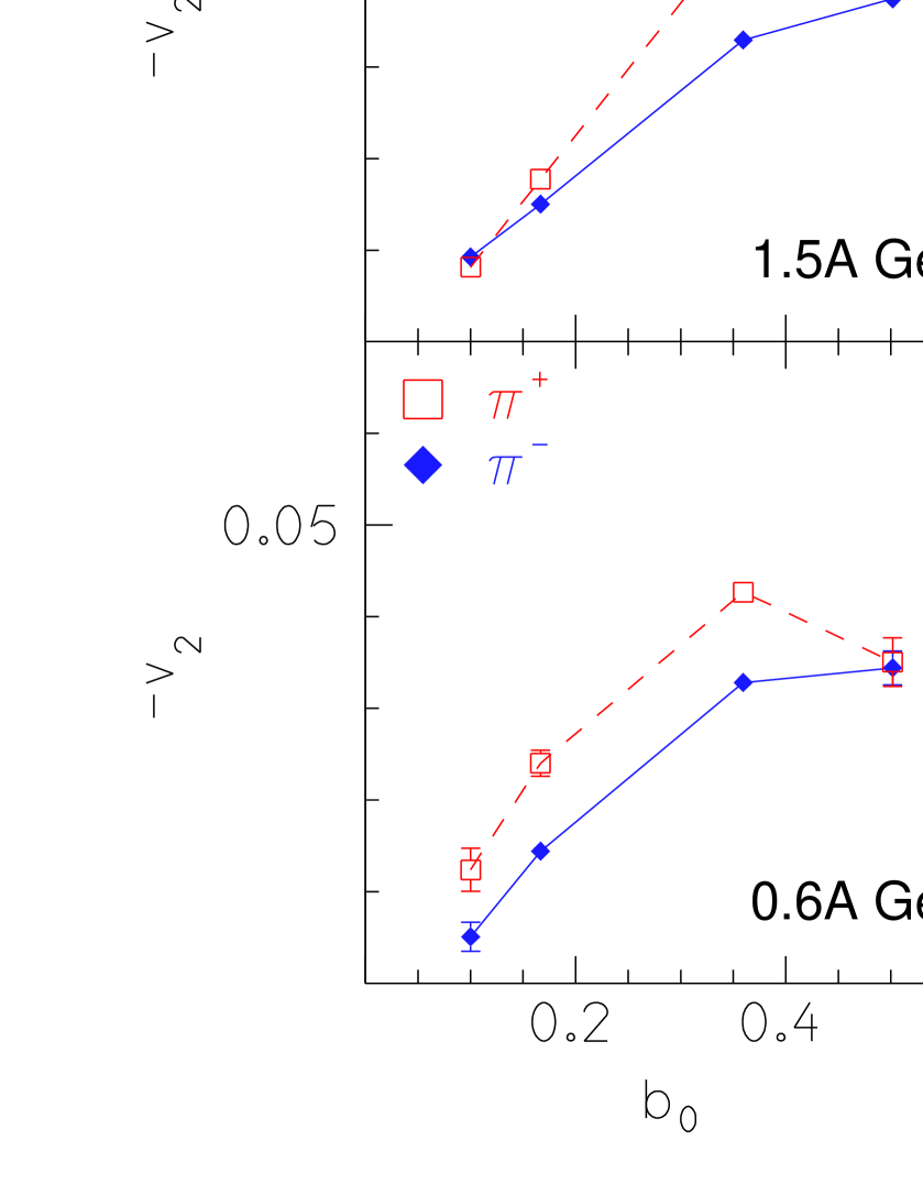
Figure 38: Centrality dependence of large acceptance elliptic flow $v_{2}$ ($-1.8<y_{0}<0$ and $1<u_{t0}<4.2$) at various indicated beam energies in the reaction Au+Au. Open squares joined by dashed lines: $\pi^{+}$, full diamonds: $\pi^{-}$.

Beam energy dependences, system size and system isospin dependences are established again in terms of large acceptance flow. The outcome is summarized in Figs. 38, 39, 40. Like $v_{1}$, $v_{2}$ evolves only slowly with energy (Fig. 38), $\pi^{+}$ elliptic flow always being somewhat larger then $\pi^{-}$ flow. The size dependence of $v_{2}$ is rather pronounced (Fig. 39) and regular in contrast to $v_{1}$ (Fig. 32). Comparing the systems ⁹⁶Ru+⁹⁶Ru and ⁹⁶Zr+⁹⁶Zr, Fig. 40, one can make the same comments as for $v_{1}$, Fig. 33. The $\pi^{+}-\pi^{-}$ difference is larger for the system with the smaller $N/Z$. If we parameterize the $b_{0}$ dependence by (one-parameter) straight lines constrained to pass the origin, we see already by eye inspection (see Fig. 40) that the difference between the two systems in terms of isospin differential flow is larger than expected naively on account of the $10\%$ Coulomb potential difference. Using the slopes of these least squares fitted lines, we can put this in a quantitative form. For $v_{2}$ the slope difference ($\pi^{+}-\pi^{-}$) is $0.0127\pm 0.0033$ (Zr+Zr) versus $0.0221\pm 0.0029$ (Ru+Ru), and for $u_{y}^{2}-u_{x}^{2}$ it is $0.054\pm 0.020$ (Zr+Zr) versus $0.106\pm 0.010$ (Ru+Ru). These observations suggest that a more extensive theoretical analysis of such data could help establishing constraints on isospin dependences of high density mean fields.

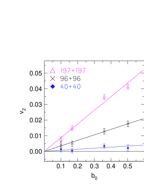
Figure 39: Centrality dependence of elliptic flow, $v_{2}$, ($-1.8<y_{0}<0$ and $0.8<u_{t0}<4.2$) for various indicated system masses. The flow is averaged over $\pi^{+}$ and $\pi^{-}$. The values for $A_{p}+A_{t}=96+96$ are an average between Zr+Zr and Ru+Ru. The straight lines are linear least square fits constrained to $v_{2}=0$ for $b_{0}=0$.

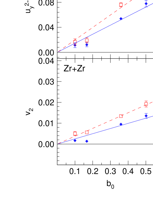
Figure 40: Comparison of the centrality dependence of elliptic flow ($v_{2}$ bottom and $u_{y}^{2}-u_{x}^{2}$ top) in the systems ⁹⁶Zr+⁹⁶Zr (left) and ⁹⁶Ru+⁹⁶Ru ($-1.8<y_{0}<0$ and $0.8<u_{t0}<4.2$). Open squares joined by dashed lines: $\pi^{+}$, full diamonds: $\pi^{-}$. The straight lines are linear least square fits constrained to $v_{2}=0$ for $b_{0}=0$.

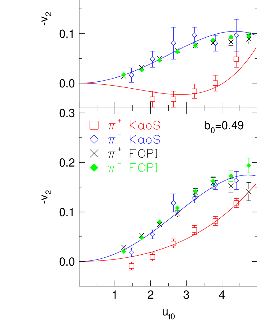
Figure 41: Transverse momentum dependence of elliptic pion flow, $v_{2}(u_{t0})$, for incident beam energies of $1A$ GeV and various indicated centralities $b_{0}$. The FOPI data for Au+Au are compared to the KaoS data [84] for Bi+Bi. The smooth curves are least squares fits of the two-parameter polynomial $v_{22}u_{t0}^{2}+v_{24}u_{t0}^{4}$ to the KaoS data guiding the eye. The data are taken in the rapidity interval $|y_{0}|<0.5$.

We close this subsection by comparing our data first to KaoS data [84] and then to IQMD simulations. KaoS published elliptic flow data for Bi+Bi at 0.4, 0.7 and $1A$ GeV. As we do not have data at $0.7A$ GeV, and since the statistical significance of our measurements at $0.4A$ GeV is rather modest, we limit ourselves to a comparison at $1A$ GeV ignoring the difference between the systems Bi+Bi and Au+Au. The comparison is shown in Fig. 41 for three centralities which were dubbed MUL2 ($b_{0}=0.66$), MUL3 ($b_{0}=0.49$) and MUL4 ($b_{0}=0.29$) in ref. [84]. (The centrality selection of KaoS is based on charged particle multiplicities registered in a 96-units hodoscope at polar angles between $12^{\circ}$ and $48^{\circ}$.) Again, we try to align the experimental conditions as much as possible, choosing similar nominal centralities and rapidity cuts for our analysis. The plotted KaoS data were inferred from Tables 1 and 2 of ref. [84] which tabulate $P_{2}=2v_{2}$ values uncorrected for resolution and then corrected using correction factors from Table 4 of ref. [88]. The average $b_{0}$ were inferred from Table 2 [88] using $b_{0}=b/R$ with $R=13.468$ fm for Bi+Bi. The shown KaoS data can be smoothened by a polynomial fit (see caption Fig. 41).

We find an excellent agreement of the data for $\pi^{-}$ flow, but not for $\pi^{+}$ flow at $b_{0}=0.29$ and $0.49$. This is somewhat puzzling as the authors of ref. [84] stress that their data show no significant difference in the azimuthal emission pattern of positively and negatively charged pions. Under the conditions chosen to generate Fig. 41 (i.e. limiting the rapidity range to $|y_{0}|<0.5$) we indeed find that $\pi^{+}$ and $\pi^{-}$ flow are very similar, although integration over a larger $y_{0}$ interval reveals a small enhancement of $\pi^{+}$ flow as we saw above. We also note that another statement in ref. [84] that ’the pion data indicate little dependence on the impact parameter’ is not properly characterizing our data for $b_{0}\leq 0.5$.

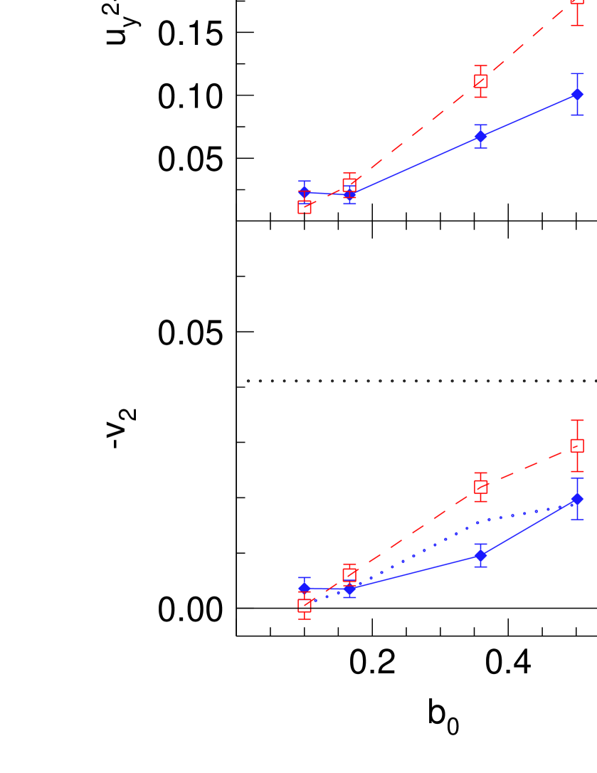
Figure 42: Centrality dependence of elliptic flow in the reaction Au+Au at $1.5A$ GeV (squares and dashed lines: $\pi^{+}$, full diamonds: $\pi^{-}$). Going from left to right, the middle panels (’FOPI’) represent the measured data for $v_{2}$, $u_{y}^{2}-u_{x}^{2}$ and the isospin differential flow $D(u_{y}^{2}-u_{x}^{2})$. The left (right) hand panels are the simulated data using a soft (stiff) equation of state. The dotted horizontal lines are references to guide the eye. The result of a linear least squares fit to the experimental isospin-differential flow (top middle flow) is repeated in the adjacent upper panels. The dotted curve in the lower left panel results from a calculation (for $\pi^{-}$) with the phase shift prescription.

In Fig. 42 we present a comparison of measured elliptic flow with results from simulations. Following a similar line as for directed flow (Fig. 35) we present large acceptance data for $(-v_{2})$, $(u^{2}_{y0}-u^{2}_{x0})$ and isospin differential $(\pi^{+}-\pi^{-})$ flow, $D(u^{2}_{y0}-u^{2}_{x0})$, in Au on Au collisions at $1.5A$ GeV framed by simulations using a soft (left panels) and stiff (right panels) EOS. Qualitatively, the trends of the simulations are similar to those of the data, the stiff EOS again being somewhat closer to the data, although still a little on the short side. The systematic $\pi^{+}-\pi^{-}$ difference is well reproduced, see the upper row of panels in Fig. 42. As already noticed for directed flow (Fig. 35), the phase shift prescription for the $\Delta$ baryon lifetime leads to a moderate (and statistically marginal) modification of the predicted elliptic flow (dotted curve in the lower left panel for $\pi^{-}$).

10 Summary

This work presents for the SIS energy regime of heavy ion collisions the most encompassing pion systematics available today. While some of the presented data are just a (needed) confirmation of earlier pioneering work, a significant number of observations are new.

Among the data which urgently needed a confirmation, are pion multiplicities. One important conclusion from our present study is that two pion detection systems that were able to measure and publish pion multiplicities in heavy ion reactions in the $1A$ GeV regime with acceptances close to $4\pi$, the BEVALAC Streamer Chamber and FOPI at SIS/Darmstadt, now offer highly consistent results (Fig. 15). In the larger framework of using heavy ion collision data to infer properties of nuclear matter far off the ground state, this should encourage future theoretical efforts to understand pion production in the $1A$ GeV regime on a level of $10\%$, the experimental uncertainty that is, presently still, typical for most absolute pion observables, and in particular the multiplicities. Extending the truly pioneering Streamer Chamber data, our present data give information on two pion charges, $\pi^{+}$ and $\pi^{-}$, and hence do not require non-trivial assumptions on the isospin dependences in order to deduce the multiplicity of all pions.

Also, our systematics in terms of system sizes and system isospin is now enlarged. As a result of this improvement, we can now say that pion multiplicities per participant are not strictly a constant for a given incident energy, but show a measurable trend towards smaller values as the participant number is increased, an effect that on the $10\%$ level does not depend on how the system size is varied, be it by varying the overlap zone changing the centrality, or by modifying target and projectile (Fig. 18).

Most of the progress since the eighties, however, rests on the detailed, centrality selected truly three-dimensional momentum space populations that have now become available. In contrast with just integrated $4\pi$ multiplicities which require large (and well understood) acceptances rather than a multitude of registered events, many subtle and relatively small effects, such as asymmetries in pion emission, required electronic devices such as FOPI to be able to handle the wealth of information connected with the variation of energy, centrality, system size and system isospin. Complemented with the studies of the TAPS and the KaoS Collaborations there now exists a rather complete set of informations on pion emission.

In two (scaled) dimensions, longitudinal rapidity, $y_{0}$, and transverse four-velocity, $u_{t0}$, the pions peak at mid-rapidity populating, especially at low energy, a rather broad phase space extending over at least twice the original rapidity gap. In these scaled units the distributions become significantly more compact at the higher end of the studied energy range (Fig. 6).

Rather than presenting the longitudinal (beam) direction in terms of a rapidity distribution on a linear scale, and then switch to a logarithmic ordinate scale to present the transverse direction in terms of a transverse mass or momentum distribution, as is commonly done in the literature, we have compared the two orthogonal directions more directly introducing the (one-dimensional) transverse rapidity distributions. The scaled variances of the transverse and the longitudinal rapidity distributions decrease significantly with increasing beam energy (Fig. 7), the transverse variance always being the smaller of the two. We have dubbed the ratio of the transverse to the longitudinal variance ’stopping’ and find that this observable decreases steadily with increasing incident energy, although more slowly than the individual variances, which in a naive thermal model (equilibrium, no flow, no decay distortions) would relate directly to (kinetic) temperatures and would have to be independent of the direction.

This ’pion stopping’ qualitatively follows the ’nucleon stopping’ [48], the latter decreasing however faster with energy, probably a reflection, on average, of a less violent collision history, due in part to a less perfect separation of spectator type influences. However, we also found evidence for spectator influence on the pions, although created particles originate in this energy regime from the overlap zone. When studying the size dependence of pion stopping, we found a remarkable phenomenon of two stopping branches: while stopping in the most central collisions is almost independent of the system size, very much in contrast to nucleon stopping [48], and even seems to increase slightly as the size decreases, an effect that is highly non-trivial, we find that stopping decreases when significant spectator matter is present (i.e. in half-overlap, $b_{0}=0.5$, collisions). We associate this observation (Fig. 8) tentatively to a reacceleration of pions penetrating and rescattering in the fast spectator (in the c.o.m. system). Since there was no significant indication of two corresponding branches in pion production, one is tempted to conclude that pions are rescattered, rather than absorbed by spectator matter.

Isospin dependence of pion stopping was not observed on a detectable level when comparing ⁹⁶Ru + ⁹⁶Ru with ⁹⁶Zr + ⁹⁶Zr.

The partial transparency that is suggested by the observation that the ’stopping’ observable is always less than one, is also evidenced by a marked polar anisotropy of pion emission (Fig. 9) which again shows the two branches depending on the presence or absence of spectators (Fig. 11). Anisotropies imply that extrapolations of midrapidity data to $4\pi$ that assume isotropic emission underestimate pion yields typically by a factor 1.2 to 1.4. When we apply this correction factor to TAPS or KaoS midrapidity data, we find fair agreement with the data from large acceptance devices, however some problem cases remain (Figs. 16, 18).

Our transverse momentum spectra, that agree in shape with KaoS (Fig. 22), and also with the IQMD simulation (Fig. 23), are characterized, besides the variance (or apparent transverse temperature) by a marked difference between $\pi^{+}$ and $\pi^{-}$ that is suggested by the simulation to originate almost exclusively from the Coulomb fields (Fig. 23). The latter also account for the main features of the systematics of ratios of average momenta (Fig. 24).

Whether the symmetry part of the ground state EOS influences the yield ratios of $\pi^{-}$ to $\pi^{+}$ in neutron rich nuclei is not clear. The naive expectation from the first chance isobar model that this ratio should grow quadratically with $N/Z$ is generally not fulfilled, as the ratio tends to vary linearly with $N/Z$ due to a partial thermalization effect, except at the lowest energy ($0.4A$ GeV). Simulations seem to miss this low energy trend, however (Figs. 25, 26).

This work also provides a significant extension of data on pion azimuthal correlations, especially for the directed flow which is of special interest due to its apparent sensitivity to the EOS (Fig. 35) [9].

The rapidity dependence $v_{1}(y_{0})$ has the S-shape familiar from the early days of flow measurements [89] and is well described in terms of an odd polynomial in $y_{0}$ including just a linear and a cubic term (Fig. 29). In contrast to the ultrarelativistic regime [87] where the flow of pions appears to be mostly opposite to proton flow (’antiflow’), we find in the $1A$ GeV regime a more complex behaviour. First, for high centralities, $b_{0}<0.4$, the flow of the pions follows the nucleon flow although it is considerably smaller in terms of $v_{1}$, roughly by the ratio of pion to nucleon mass. For larger impact parameters there is a switch to antiflow (Figs. 29 and 34). Second, the flow of positively charged pions differs from that of negatively charged pions, in particular the switch to antiflow occurs at smaller centrality (Fig. 34).

Although these features confirm qualitatively what was found in an earlier study by the EOS Collaboration [80], the quantitative agreement is not satisfactory (Fig. 34): whether the difference is due to different detector acceptances is not clear.

The transverse velocity dependence $v_{1}(u_{t0})$ (integrated over a large rapidity interval) is relatively flat with weak structures (Fig. 30).

Despite theses detailed features which show that pion flow is a complex phenomenon, it is useful for systematics purposes to try to characterize flow by just one parameter. One alternative is the midrapidity slope $dv_{1}/dy_{0}(y_{0}=0)$, for which we have established a systematics varying the incident energy (Fig. 31): this parameterization puts more weight on the midrapidity region. Another alternative, stressing higher rapidities, consists of the large-acceptance value of $v_{1}$, for which we have established size (Fig. 32) and isospin (Fig. 33) dependences. The isospin differential flow of pions is a systematic effect which is largest for Au + Au at the lower incident energies (Fig. 31). It seems to be dominated by Coulomb effects since it is quantitatively reproduced by our simulation for Au+Au at $1.5A$ GeV (Fig. 35) which did not include isospin dependent mean fields except for the Coulomb field. However, surprisingly, the isospin differential pion flow was found to be significantly smaller for ⁹⁶Zr + ⁹⁶Zr ($N/Z=1.40$) than for ⁹⁶Ru + ⁹⁶Ru ($N/Z=1.18$), Fig. 33. Quantitatively, it seems necessary to introduce a nuclear isospin field of opposite sign to the Coulomb part of the field in order to explain this feature. The simulation at $1.5A$ GeV (Fig. 35) showed that the EOS influences pion directed flow in a measurable way, favouring the stiffer EOS in the IQMD version that we used.

In the $1A$ GeV energy range pion elliptic flow like nucleonic flow is negative, i.e. preferentially out-of plane . The presence of spectator matter in the expansion phase of the fireball is probably the most important ’geometrical’ difference to the ultrarelativistic regime [87], our stopping studies indicating that pion rescattering in spectator matter plays a role, as was already suggested in ref. [33]. We find that $v_{2}(y_{0})$ is rather flat over a very large range of rapidities (Fig. 36). In contrast to directed flow, $|v_{2}|$ increases nearly linearly with decreasing centrality in the range covered by our data ($b_{0}<0.55$). The transverse four-velocity dependence $v_{2}(u_{t0})$ (Fig. 37) is quadratic ($\pi^{-}$) or linear ($\pi^{+}$) for smaller momenta, flattening out at higher momenta. We confirm the tabulated KaoS data [84] for $\pi^{-}$ (Fig. 41), but not for $\pi^{+}$. While the dependence on incident energy is relatively weak, Fig. 38, the system-size dependence is rather strong for all centralities, Fig. 39. As for directed flow, the system ⁹⁶Ru + ⁹⁶Ru shows a larger difference between $\pi^{+}$ and $\pi^{-}$ elliptic flow than the system ⁹⁶Zr + ⁹⁶Zr, so the same comments apply. In comparing with the IQMD simulations we find experimentally a somewhat larger elliptic flow, even when using the stiff EOS (Fig. 42). The isospin differential flow in the heavy system Au+Au is again well reproduced (Fig. 40).

At this time, however we do not wish to draw firm conclusions on the issue of the stiffness of the EOS from the pion flow, as we expect other features of the simulation, namely the treatment of the $\Delta$ baryon propagation in the medium, to influence the predicted flow. Shorter effective $\Delta$ baryon lifetimes in the model are expected to decrease the efficiency of the assumed dominant pion absorption mechanism via $N\Delta\rightarrow NN$ and hence the pion yields at freeze out, as well as the influence of the mean field in the time between elementary collisions, and hence the observed flow. This is an interesting aspect of in-medium physics in its own right and deserves theoretical investigations with the aim of reaching a consensus on how this problem should be treated properly in transport codes.

Much work still needs to be done, to coordinate the transport theoretical efforts with the aim of achieving code independent conclusions. Such efforts were started in ref. [27] and continued on a larger scale in ref. [64] which also contains further literature citations (and transport codes) for the interested reader

The request for reproduction of finer details, such as the full 3D features of the momentum space population under exclusive conditions, subtle system size and isospin effects, is premature at this time as long as global features, such as production, stopping and integrated flow are not under sufficient control. This is a task for future theoretical work beyond the scope of the present experimental work. From the richness of our observations it follows that this represents a challenge and hopefully will eventually contribute to a better understanding of nuclear medium properties, which cannot simply be inferred from incoherently superimposing experimental information on so-called ’elementary’ hadron-hadron reactions.

References

- [1] T.-S. Lee, R. P. Redwine, Annu. Rev. Nucl. Part. Sci. 52 (2002) 23.
- [2] R. S. Mayer, et al., Phys. Rev. Lett. 78 (1997) 4165).
- [3] G. F. Bertsch, S. Das Gupta, Phys. Rep. 160 (1988) 189.
- [4] J. W. Harris, et al., Phys. Rev. Lett. 58 (1987) 463.
- [5] R. Stock, Phys. Rep. 135 (1986) 259.
- [6] G. F. Bertsch, H. Kruse, S. Das Gupta, Phys. Rev. C 29 (1984) 673.
- [7] H. Kruse, B. V. Jacak, H. Stöcker, Phys. Rev. Lett. 54 (1985) 289.
- [8] Y. Kitazoe, M. Sano, H. Toki, S. Nagamiya, Phys. Lett. B 166 (1986) 35.
- [9] S. A. Bass, C. Hartnack, H. Stöcker, W.Greiner, Phys. Rev. C 51 (1995) R12.
- [10] S. Y. Fung, et al., Phys. Rev. Lett. 52 (1978) 292.
- [11] A. Sandoval, et al., Phys. Rev. Lett. 45 (1980) 874.
- [12] J. W. Harris, et al., Phys. Lett. B 153 (1985) 377.
- [13] J. P. Alard, et al., Nucl. Instr. Meth. A 261 (1987) 379.
- [14] A. Gobbi, et al., Nucl. Instr. Meth. A 324 (1993) 156.
- [15] J. Ritman, Nucl. Phys. B 44 (1995) 708.
- [16] H. Wieman, et al., Nucl. Phys. A 525 (1991) 617c.
- [17] P. Senger, et al., Nucl. Instr. Meth. A 327 (1993) 393.
- [18] R. Novotny, IEEE Trans. Nucl. Sci. 38 (1991) 379.
- [19] P. Senger, H. Ströbele, J. Phys. G 25 (1999) R59.
- [20] D.Pelte, et al., Z. Phys. A 357 (1997) 215.
- [21] D.Pelte, et al., Z. Phys. A 359 (1997) 55.
- [22] B. Hong, et al., Phys. Lett. B 407 (1997) 115.
- [23] B. Hong, et al., Phys. Rev. C 57 (1998) 244.
- [24] B. Hong, et al., Phys. Rev. C 71 (2005) 034902.
- [25] Marc R. Stockmeier, Ph.D thesis, University of Heidelberg (2002), Germany.
- [26] W. Reisdorf, et al., Nucl. Phys. A 612 (1997) 493.
- [27] C. Hartnack, et al., Eur. Phys. J. A 1 (1998) 151.
- [28] J. Aichelin, Phys. Rep. 202 (1991) 233.
- [29] S. A. Bass, C. Hartnack, R. Mattiello, H. Stöcker, W.Greiner, Phys. Lett. B 302 (1993) 381.
- [30] S. A. Bass, C. Hartnack, H. Stöcker, W.Greiner, Phys. Rev. Lett. 71 (1993) 1144.
- [31] S. A. Bass, C. Hartnack, H. Stöcker, W.Greiner, Phys. Rev. C 50 (1994) 2167.
- [32] S. A. Bass, M. Hofmann, C. Hartnack, H. Stöcker, W.Greiner, Phys. Lett. B 335 (1994) 289.
- [33] S. A. Bass, C. Hartnack, H. Stöcker, W.Greiner, Phys. Rev. C 51 (1995) 3343.
- [34] S. A. Bass, C. Hartnack, H. Stöcker, W.Greiner, Z. Phys. A 351 (1995) 359.
- [35] E. L. Hjort, et al., Phys. Rev. Lett. 79 (1997) 4345.
- [36] M. Eskef, et al., Eu. Phys. J A 3 (1998) 335.
- [37] T. Matulewicz, et al., Eur. Phys. J. 9 (2000) 69.
- [38] Bao-An Li, C. B. Das, S. Das Gupta and C. Gale, Phys. Rev. C 69 (2004) 011603(R); Nucl. Phys. A 735 (2004) 563.
- [39] V. Baran, M. Colonna, V. Greco, and M. Di Toro, Phys. Rep. 410 (2005) 335.
- [40] T. Gaitanos, et al., Nucl. Phys. A 650 (1999) 97; C. Fuchs, T. Gaitanos, Nucl. Phys. A 714 (2003) 643.
- [41] W. Cassing, S. Juchem, Nucl. Phys. A 665 (2000) 377; Nucl. Phys. A 672 (2000) 417; Nucl. Phys. A 677 (2000) 445.
- [42] A. B. Larionov, U. Mosel, Nucl. Phys. A 728 (2003) 135.
- [43] P. Danielewicz, Phys. Rev. C 51 (1995) 716.
- [44] Qingfeng Li, Zhuxia Li, Sven Soff, Marcus Bleicher, Horst Stöcker, J. Phys. G. 32 (2006)151.
- [45] S. A. Bass, et al., Prog. Part. Nucl. Phys. 41 (1998) 255.
- [46] W. Reisdorf, et al., Phys. Lett. B 595 (2004) 118.
- [47] GEANT-Detector description and Simulation Tool, CERN program library Long Writeup W5013 (CN Division, CERN, 1993).
- [48] W. Reisdorf, et al., Phys. Rev. Lett. 92 (2004) 232301.
- [49] R. Averbeck, R. Holzmann, V. Metag, R. S. Simon, Phys. Rev. C 67 (2003) 024903.
- [50] K. L. Wolf, et al., Phys. Rev. Lett. 42 (1979) 1448.
- [51] S. Nagamiya, et al., Phys. Rev. C 24 (1981) 971; J. Chiba, et al., Phys. Rev. C 20 (1979) 1332; K. Nakai, et al., Phys. Rev. C 20 (1979) 2210.
- [52] R. Holzmann, et al. (TAPS Collaboration), Phys. Lett. B 366 (1996) 63.
- [53] K. Tymińska, T. Matulewicz, K. Piasecki (TAPS Collaboration), Acta Phys. Polonica B 37 (2006) 161.
- [54] R. Brockmann, et al., Phys. Rev. Lett. 53 (1984) 2012.
- [55] J. Gosset, et al., Phys. Rev. C 16 (1977) 629.
- [56] R. Stock, et al., Phys. Rev. Lett. 49 (1982) 1236.
- [57] A. Wagner, Phd thesis, University of Darmstadt (1996) (in German).
- [58] G. Martinez, et al., Phys. Rev. Lett. 83 (1999) 1538.
- [59] R. Averbeck, et al., Z. Phys. A 359 (1997) 65.
- [60] M. Gazdzicki, D. Röhrich, Z. Phys. C 65 (1995) 215.
- [61] O. Schwalb, et al., Phys. Lett. B 321 (1994) 20.
- [62] D. Ashery, I. Navon, G. Azuelos, H. K. Walter, H. J. Pfeiffer, F. W. Schlepütz, Phys. Rev. C 23 (1981) 2173.
- [63] L. Ahle, et al., Phys. Lett. B 476 (2000) 1.
- [64] E. E. Kolomeitsev, et al., J. Phys. G 31 (2005) S741.
- [65] E. P. Wigner, Phys. Rev. 98 (1955) 145.
- [66] P. Danielewicz, S. Pratt, Phys. Rev. C 53 (1996) 249.
- [67] E. N. E. van Dalen, C. Fuchs, A. Faessler, Phys. Rev. Lett. 95 (2005) 022302.
- [68] F. Uhlig (KaoS Collaboration), private communication.
- [69] A. Wagner, et al., Phys. Lett. B 420 (1998) 20.
- [70] Bao-An Li, Phys. Rev. C 67 (2003) 017601.
- [71] T. Gaitanos, M. Di Toro, S. Typel, V. Baran, C. Fuchs, V. Greco, H. H. Wolter, Nucl. Phys. A 732 (2004) 24.
- [72] J. J. Kapusta, Phys. Rev. C 16 (1977) 1493.
- [73] H. A. Gustafsson, et al., Phys. Rev. Lett. 52 (1984) 1590.
- [74] R. E. Renfordt, et al., Phys. Rev. Lett. 53 (1984) 763.
- [75] P. Danielewicz, G. Odyniec, Phys. Lett. B 157 (1985) 168.
- [76] J.-Y. Ollitrault, Nucl. Phys. A 638 (1998) 195c.
- [77] R. S. Bhalerao, N. Borghini, J.Y. Ollitrault, Nucl. Phys. A 727 (2003) 373; Phys. Lett. B 580 (2004) 157.
- [78] N. Bastid et al., Phys. Rev. C 72 (2005) 011901 and to be published.
- [79] J. Gosset, et al., Phys. Rev. Lett. 62 (1989) 1251.
- [80] J. C. Kintner et al., Phys. Rev. Lett. 78 (1997) 4165.
- [81] Bao-An Li, Nucl. Phys. A 570 (1994) 797.
- [82] D. Brill, et al., Phys. Rev. Lett. 71 (1993) 336.
- [83] L. B. Venema, et al., Phys. Rev. Lett. 71 (1993) 835.
- [84] D. Brill, et al., Z. Phys. A 357 (1997) 207.
- [85] A. Wagner, et al., Phys. Rev. Lett. 85 (2000) 18.
- [86] J. Barrette, et al. (E877 Collaboration), Phys. Rev. C 55 (1997) 1420.
- [87] C. Alt, et al. (NA49 Collaboration), Phys. Rev. C 68 (2003) 034903.
- [88] D. Brill, et al., Z. Phys. A 355 (1996) 61.
- [89] W. Reisdorf, H. G. Ritter, Annu. Rev. Nucl. Part. Sci. 47 (1997) 663; N. Herrmann, J. P. Wessels, T. Wienold, ib. 49 (1999) 581.