Measurement of the $\nu_{e}$ and Total ⁸B Solar Neutrino Fluxes with the Sudbury Neutrino Observatory Phase I Data Set

Abstract

This article provides the complete description of results from the Phase I data set of the Sudbury Neutrino Observatory (SNO). The Phase I data set is based on a 0.65 kt-year exposure of heavy water to the solar ⁸B neutrino flux. Included here are details of the SNO physics and detector model, evaluations of systematic uncertainties, and estimates of backgrounds. Also discussed are SNO’s approach to statistical extraction of the signals from the three neutrino reactions (charged current, neutral current, and elastic scattering) and the results of a search for a day-night asymmetry in the $\nu_{e}$ flux. Under the assumption that the ⁸B spectrum is undistorted, the measurements from this phase yield a solar $\nu_{e}$ flux of $\phi(\nu_{e})=1.76^{+0.05}_{-0.05}\mbox{(stat.)}^{+0.09}_{-0.09}~{}\mbox{(syst.)}\times 10^{6}$ cm^-2 s^-1, and a non-$\nu_{e}$ component $\phi(\nu_{\mu\tau})=3.41^{+0.45}_{-0.45}\mbox{(stat.)}^{+0.48}_{-0.45}~{}\mbox{(syst.)}\times 10^{6}$ cm^-2 s^-1. The sum of these components provides a total flux in excellent agreement with the predictions of Standard Solar Models. The day-night asymmetry in the $\nu_{e}$ flux is found to be $A_{e}=7.0\pm 4.9~{}\mathrm{(stat.)^{+1.3}_{-1.2}}\%~{}\mathrm{(sys.)}$, when the asymmetry in the total flux is constrained to be zero.

I Introduction

More than thirty years of solar neutrino experiments cl ; kam ; sage ; gallex ; SK ; gno indicated that the total flux of neutrinos from the Sun was significantly smaller than predicted by models of the Sun’s energy generating mechanisms BP01 ; TC . The deficit was not only universally observed but had an energy dependence which was difficult to attribute to astrophysical sources. The data were consistent with a negligible flux of neutrinos from solar ⁷Be hata ; hamish , though neutrinos from ⁸B (a product of solar ⁷Be reactions) were observed. A natural explanation for the observations was that neutrinos born as $\nu_{e}$s change flavor on their way to the Earth, thus producing an apparent deficit in experiments detecting primarily $\nu_{e}$s. Neutrino oscillations—either in vacuum pontecorvo ; mns or matter wolf ; ms —provide a mechanism both for the flavor change and the observed energy variations.

While these deficits argued strongly for neutrino flavor change through oscillation, it was clear that a far more compelling demonstration would not resort to model predictions but look directly for neutrino flavors other than the $\nu_{e}$ emitted by the Sun. The Sudbury Neutrino Observatory (SNO) was designed to do just that: provide direct evidence of solar neutrino flavor change through observation of non-electron neutrino flavors by making a flavor-independent measurement of the total ⁸B neutrino flux from the Sun hhchen . As a real-time detector, SNO was also designed to look for specific signatures of the oscillation mechanism, such as energy- or time-dependent survival probabilities. For example, depending upon the values of the mixing parameters, the matter (MSW) effect leads to different $\nu_{e}$ fluxes during the day and the night and to a distortion in the expected energy spectrum of ⁸B solar neutrinos.

We present in this article the details of the analyses presented in previous SNO publications SNO Collaboration (2001, 2002a, 2002a), including the exclusive $\nu_{e}$ and inclusive active neutrino fluxes, a measurement of the $\nu_{e}$ spectrum, the difference in the neutrino fluxes between day and night, and determination of the neutrino mixing parameters. We will concentrate here on the low-energy threshold measurements of Refs. SNO Collaboration (2002a, a) which included the first measurements of the total ⁸B flux, but will describe the differences between these analyses and the high-threshold measurement presented in Ref. SNO Collaboration (2001).

We begin in Section II with an overview of the SNO detector and data analysis. In Section III we describe the data set used for the measurements made in the initial phase (hereafter Phase I) of SNO using pure D₂O as the target-detector. Section IV describes the detector model which is ultimately used both to calibrate the neutrino data and to provide distributions used to fit our data. Section V describes the processing of the data, including all cuts applied, reconstruction of position and direction, and estimations of effective kinetic energy for each event. Section VI details the systematic uncertainties in the model, which translate into uncertainties in the neutrino fluxes. Section VII describes the measurement of backgrounds remaining in the data set, including neutrons from photodisintegration, the tails of low energy radioactivity, and cosmogenic sources. Section VIII details the methods used to fit for the neutrino rates, and Section IX the ingredients which go into normalization of the rates. Sections X and XI present the flux results and results of a search for an asymmetry in the day and night fluxes. Appendix XIV describes the methods used to calculate mixing parameters from these data, and Appendix XV gives details of the cuts we used to remove instrumental backgrounds.

We will refer in this article to Ref. SNO Collaboration (2001) as the ‘ES-CC paper’, Ref. SNO Collaboration (2002a) as the ‘NC paper’, Ref. SNO Collaboration (2002a) as the ‘Day-Night paper’, and collectively we call them the ‘Phase I publications’.

II Overview of SNO

II.1 The SNO Detector

SNO is an imaging Cherenkov detector using heavy water (D₂O) as both the interaction and detection medium NIM . SNO is located in Inco’s Creighton Mine, at $46^{\circ}28^{{}^{\prime}}30^{{}^{\prime\prime}}$ N latitude, $81^{\circ}12^{{}^{\prime}}04^{{}^{\prime\prime}}$ W longitude. The detector resides 1730 m below sea level with an overburden of 6020 meters water equivalent, deep enough that the rate of cosmic ray muons passing through the entire active volume is just 3 per hour.

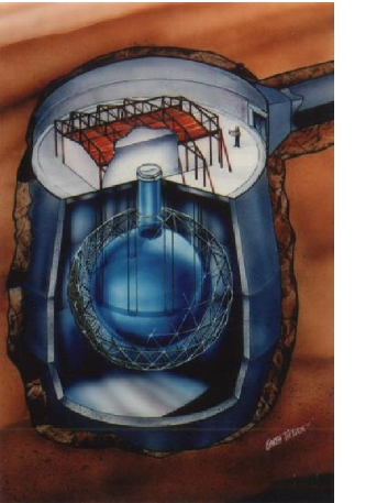
Figure 1: Schematic of SNO Detector.

Figure 1 is a schematic of the detector. One thousand metric tons of heavy water are contained in a 12-m diameter transparent acrylic vessel (AV). Cherenkov light produced by neutrino interactions and radioactive backgrounds is detected by an array of 9456 Hammamatsu model R1408 8-inch photomultiplier tubes (PMTs), supported by a stainless steel geodesic sphere (the PMT support sphere or PSUP). Each PMT is surrounded by a light concentrator (‘reflector’), which increases the photocathode coverage to nearly $55$%. The channel discriminator thresholds are set to fire on 1/4 of a photoelectron of charge. Over seven kilotons of light water shield the heavy water from external radioactive backgrounds: 1.7 kT between the acrylic vessel and the PMT support sphere, and 5.7 kT between the PMT support sphere and the surrounding rock. The 5.7 kT of light water outside the PMT support sphere is viewed by 91 outward-facing 8-inch PMTs that are used for identification of cosmic-ray muons. An additional 23 PMTs, arranged in a rectangular array, are suspended in the outer light water region. These 23 PMTs view the neck of the acrylic vessel and are used primarily in the rejection of instrumentally generated light.

The detector is equipped with a versatile calibration deployment system which can place radioactive and optical sources over a large range of the $x$-$z$ and $y$-$z$ planes in the AV. Sources that can be deployed include a diffuse multi-wavelength laser for measurements of PMT timing and optical parameters laserball , a ¹⁶N source which provides a triggered sample of 6.13 MeV $\gamma$s n16 , and a ⁸Li source that delivers tagged $\beta$s with an endpoint near 14 MeV li8 . In addition, high energy (19.8 MeV) $\gamma$s are provided by a ${}^{3}{\rm H}(p,\gamma)^{4}{\rm He}$ (‘pT’) source poon and neutrons by a ²⁵²Cf source. Some of the sources can also be deployed on vertical axes within the light water volume between the acrylic vessel and PMT support sphere.

II.2 Physics Processes in SNO

SNO was designed to provide direct evidence of solar neutrino flavor change through comparisons of the interaction rates of three different processes:

$\nu_{x}+e^{-}\rightarrow\nu_{x}+e^{-}$	(ES)
$\nu_{e}+d\rightarrow p+p+e^{-}$	(CC)
$\nu_{x}+d\rightarrow p+n+\nu_{x}$	(NC)

The first reaction, elastic scattering (ES) of electrons, has been used to detect solar neutrinos in other water Cherenkov experiments. It has the great advantage that the recoil electron direction is strongly correlated with the direction of the incident neutrino, and hence the direction to the Sun $(\cos\theta_{\odot})$. This ES reaction is sensitive to all neutrino flavors. For $\nu_{e}$s, the elastic scattering reaction has both charged and neutral current components, making the cross section for $\nu_{e}$s $\sim$ 6.5 times larger than that for $\nu_{\mu}$s or $\nu_{\tau}$s.

Deuterium in the heavy water provides loosely bound neutron targets for an exclusively charged current (CC) reaction which, at solar neutrino energies, occurs only for $\nu_{e}$s. In addition to providing exclusive sensitivity to $\nu_{e}$s, this reaction has the advantage that the recoil electron energy is strongly correlated with the incident neutrino energy, and thus can provide a precise measurement of the ⁸B neutrino energy spectrum. The CC reaction also has an angular correlation with the Sun which falls as $(1-0.340\cos\theta_{\odot})$ vogel , and has a cross section roughly ten times larger than the ES reaction for neutrinos within SNO’s energy acceptance window.

The third reaction, also unique to heavy water, is a purely neutral current (NC) process. This has the advantage that it is equally sensitive to all neutrino flavors, and thus provides a direct measurement of the total active flux of ⁸B neutrinos from the Sun. Like the CC reaction, the NC reaction has a cross section nearly ten times as large as the ES reaction.

For both the ES and CC reactions, the recoil electrons are detected directly through their production of Cherenkov light. For the NC reaction, the neutrons are not seen directly, but are detected in a multi-step process. When a neutrino liberates a neutron from a deuteron, the neutron thermalizes in the D₂O and may eventually be captured by another deuteron, releasing a 6.25 MeV $\gamma$ ray. The $\gamma$ ray either Compton scatters an electron or produces an $e^{+}e^{-}$ pair, and the Cherenkov radiation of these secondaries is detected.

To determine whether neutrinos that start out as $\nu_{e}$s in the solar core convert to another flavor before detection on Earth, we have two methods: comparison of the CC reaction rate to the NC reaction rate, or comparison of the CC rate to the ES rate. The NC-CC comparison has the advantage of high sensitivity. When we compare the total flux to the $\nu_{e}$ flux, we expect the former to be roughly three times the latter if both solar neutrino experiments and standard solar models are correct. In addition, many uncertainties in the cross sections for the two processes will largely cancel.

The comparison of CC to ES has the advantage that recoil electrons from both reactions provide neutrino spectral information. The spectral information can ultimately be used to show that any excess in the ES reaction over the CC reaction is not caused by a difference in the effective neutrino energy thresholds used to analyze the two reactions fogli01 ; Villante et al. (1999). The CC-ES comparison also has the advantage that the strong angular correlation of the ES electrons with the direction to the Sun demonstrates that any excess seen is not due to some unexpected non-solar background. Lastly, the CC-ES comparison can be made using both SNO’s ES measurement and the high precision ES measurement made by the Super-Kamiokande collaboration SK . This provides a high sensitivity cross check for the CC-NC comparison with different backgrounds and systematic uncertainties.

The goal of the SNO experiment is to determine the relative sizes of the three signals (CC, ES, and NC) and to compare their rates. We cannot separate the signals on an event-by-event basis; instead, we ‘extract’ the signals statistically by using the fact that they are distributed distinctly in the following three derived quantities: the effective kinetic energy $T_{\rm eff}$ of the $\gamma$ ray resulting from the capture of a neutron produced by the NC reaction or the recoil electron from the CC or ES reactions, the reconstructed radial position of the interaction ($R^{3}$) and the reconstructed direction of the event relative to the expected direction of a neutrino arriving from the Sun ($\cos\theta_{\odot}$). We measure the radial positions in units of AV radii, so that $R^{3}\equiv(R_{\rm fit}/R_{AV})^{3}=1.0$ when an event reconstructs at the edge of the heavy-water volume.

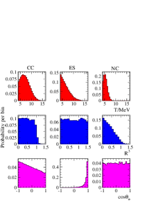
Figure 2: The energy (top row), radial (middle row), and directional (bottom row) distributions used to build pdfs to fit the SNO signal data. $T_{\rm eff}$ is the effective kinetic energy of the $\gamma$ from neutron capture or the electron from the ES or CC reactions, and $R$ is the reconstructed event radius, normalized to the 600 cm radius of the acrylic vessel.

Figure 2 shows simulated distributions for each of the signals. The top row shows the energy distributions for each of the three signals. The strong correlation between the electron energy and the incident neutrino energy for the CC interaction produces a spectrum which resembles the initial ⁸B neutrino spectrum, while the recoil spectrum for the ES reaction is much softer. The NC reaction is, within the smearing of the Compton scattering process and the resolution of the detector, essentially a line spectrum, because the $\gamma$ produced by the neutron capture on deuterium always has an energy of 6.25 MeV.

The distributions of reconstructed event positions $R^{3}$, normalized to the radius of the acrylic vessel $R_{AV}$, are shown in the middle row of Fig. 2. We see here that the CC reaction, which occurs only on deuterons, produces events distributed uniformly within the heavy water, while the ES reaction, which can occur on any electron, produces events distributed uniformly well beyond the heavy-water volume. The small leakage of events just outside the heavy-water volume (just outside $R^{3}=1$) for the CC reaction is due to the resolution tail of the reconstruction algorithm.

The NC signal, however, does not have a uniform distribution inside the heavy water, but instead decreases monotonically from the central region to the edge of the acrylic vessel. The reason for this is the long ($\sim$ 120 cm) thermal diffusion length for neutrons in D₂O. Neutrons produced near the edge of the heavy-water volume have a high probability of wandering outside it, at which point they can be captured on hydrogen either in the acrylic vessel or the H₂O surrounding the vessel. The capture cross section on hydrogen is nearly 600 times larger than on deuterium, and therefore these hydrogen captures occur almost immediately, leaving no opportunity for the neutrons to diffuse back into the fiducial volume. Further, such hydrogen captures produce a 2.2 MeV $\gamma$ ray which is well below the analysis threshold, and therefore events from these captures do not appear in the NC $R^{3}$ pdf shown in Figure 2.

The bottom row of Fig. 2 shows the reconstructed direction distribution of the events. In the middle of that row we see the peaking of the ES reaction, pointing away from the Sun. The $\sim$ $1-1/3\cos\theta_{\odot}$ distribution of the CC reaction is also clear in the left-most plot. The NC reaction shows no correlation with the solar direction—the $\gamma$ ray from the captured neutron carries no directional information about the incident neutrino.

One last point needs to be made regarding the distributions labelled ‘NC’ in Fig. 2: they represent equally well the detector response to any neutrons, not just those produced by neutral current interactions, as long as the neutrons are distributed uniformly in the detector. For example, neutrons produced through photodisintegration by $\gamma$ rays emitted by radioactivity inside the D₂O will have the same distributions of energy, radial position, and direction as those produced by solar neutrinos. These neutrons are an irreducible background in the data analysis, and must be kept small through purification of detector materials.

II.3 Analysis Strategy

To determine the sizes of the CC, ES, and NC signals we use the nine distributions of Fig. 2 to create probability density functions (pdfs) and perform a generalized maximum likelihood fit of the data to the same distributions. There are, however, three principal prerequisites before we can begin this ‘signal extraction’ process: we must process the data so that we can create distributions of event energies, positions, and directions; we need to build a model of the detector so that we can create the pdfs like those in Fig. 2; and we need to provide measurements of any residual backgrounds.

Data processing begins with the calibration of the raw data, converting ADC values into PMT charges and times. The calibrated charges and times allow us to reconstruct each event’s position and direction, as well as estimate event energy. We also apply cuts to the data set during processing to remove as many background events as possible without sacrificing a substantial number of neutrino signal events.

The signal extraction process described above implicitly assumes that the pdfs used in the fit are built from a complete and accurate representation of the detector’s true response. The model we use to create the pdfs must therefore describe everything from the physics of neutrino interactions, to the propagation of particles and optical photons through the detector media, to the behavior of the data acquisition system. The model needs to reproduce the response to signal events at all places in the detector, for all neutrino directions, for all neutrino energies, and for all times. It must also track changes in the detector over time, such as failed PMTs or electronics channels.

Although our suite of cuts is very efficient at removing background events, we nevertheless must demonstrate that the residual background levels are negligible or we must produce measurements of their size. The latter is particularly important for the photodisintegration neutrons—because they look identical to the NC signal, they cannot be removed, and must be measured and subtracted from the total neutron count resulting from the maximum likelihood fit.

Signal extraction estimates the numbers of CC, NC, and ES events; conversion to fluxes requires acceptance corrections for each of the signals and, for the NC signal, adjustments for the capture efficiency of neutrons on deuterons. The final normalization also includes neutrino interaction cross sections, detector livetime, and the number of available targets.

For our first publications we performed three independent analyses of the data presented in this article the:mgb ; the:kh ; the:msn . Prior to final processing, we chose from these three analyses two independent approaches for each major analysis component (cut sets, reconstruction algorithms, energy calibration, etc.). Comparisons of the results of the independent approaches were used to validate every component of the analysis—one approach was designated ‘primary’ and used for the Phase I published results, and one was designated ‘secondary’ and used as the verification check. Table 26 lists the approaches for each of the analysis components. In this article, we describe both the primary and secondary approaches used.

III Data Set

The data set used in the analysis we describe here was acquired between November 2, 1999 and May 31, 2001, and represents a total of 306.4 live days. Although the SNO detector is live to neutrinos during nearly all calibrations, data taken during the calibration periods—roughly 10% of the time the detector is running—is not used for solar neutrino analysis. Other losses of livetime result from mine power outages, detector maintenance periods and the loss of underground laboratory communication or environmental systems.

The SNO data set is divided into ‘runs’, a new run being started either at a change in detector conditions (such as the insertion of a calibration source) or after a maximum duration has been exceeded (in Phase I, no more than four days). The runs used for the final analysis were selected based upon criteria external to the data themselves. Selected runs were those for which calibration sources were not present in the detector, no major electronics systems were off-line, no maintenance was being performed, and no circulation of the D₂O that caused light to be produced inside the detector was being undertaken.

The SNO detector responds to several triggers, the primary one being a coincidence of 18 or more PMTs firing within a period of $\sim$ 93 ns (the threshold was lowered to 16 or more PMTs after December 20, 2000). The rate of such triggers averaged roughly 5 Hz. The detector also triggered if the total charge collected in all PMTs exceeded 150 photoelectrons. A ‘random’ trigger pulsed the detector at 5 Hz throughout the data set, and a pre-scaled trigger fired after every thousandth 11-PMT threshold crossing. Information about which condition caused the trigger for a given event was saved as part of the primary data stream. The overall trigger rate was between 15 and 20 Hz.

Although the overall detector configuration was kept stable during the data taking period, we performed two fixes worthy of comment. The first was a change to the charge- and time-digitizing analog-to-digital converters (ADCs). Soon after the start of production running, it was discovered that the ADCs were developing non-linearities well beyond their specification. During most of the data taking period, bad ADCs were periodically replaced or repaired, but on August 18, 2000, a permanent fix was implemented. In addition, roughly halfway through the data taking period, we discovered a small rate dependence to the PMT timing measurements. Although small, the rate dependence did affect our position reconstruction. We developed a hardware solution to mitigate the effect, and also created an off-line calibration to remove it. The hardware change was completed in December, 2000, and the off-line calibration was applied to the entire data set.

Other minor changes—failure of individual PMTs (at an average rate of about 1% per year), alteration of front-end discriminator thresholds, or repair of broken electronics channels—were tracked and the status of every channel was stored in the SNO database at the beginning of each run for use in the offline data analysis. In addition, the front-end electronics timing and charge responses were calibrated twice each week, much more frequently than the observed variations of pedestals or slopes. Calibration of phototube gain, timing, and risetime response was done roughly monthly.

To provide a final check against statistical bias, the data set was divided in two, an ‘open’ data set to which all analysis procedures and methods were applied, and a ‘blind’ data set upon which no analysis within the signal region (between 40 and 200 hit phototubes) was performed until the full analysis program had been finalized. The blind data set began at the end of June 2000, at which point we began analyzing just 10% of the data set, leaving the remaining 90% blind. The total size of the blind data set thus corresponded to roughly 30% of the total livetime.

IV Physics and Detector Model

Both reconstruction of event kinetic energy and construction of the distributions shown in Fig. 2 require a model of the detector’s response to Cherenkov light created by neutrino interactions. For energy reconstruction, the model we use for the response is analytical, and for the creation of the pdfs in Fig. 2 the model is a Monte Carlo simulation. Most of the required inputs are the same for both models: the physics of the passage of electrons and $\gamma$-rays through the various detector media and the associated production of Cherenkov light, the optical properties of the detector, and the state and response of the detector PMTs, electronics, and trigger. In addition, for the Monte Carlo simulation to correctly predict the energy spectra and direction distributions, it must include the total and differential cross sections for the CC, ES, and NC neutrino interactions, as well as the incident ⁸B neutrino spectrum. Lastly, to produce the correct radial distributions for the neutrons from the NC reaction, the Monte Carlo model also simulates the transport and capture of low energy ($<$20 MeV) neutrons.

In the following section, we describe the details of each component of the models and the calibrations applied. As will be seen here and in subsequent sections of this article, the Monte Carlo simulation reproduced nearly all the distributions of interest we measured with our calibration sources to a high degree of accuracy.

IV.1 Neutrino Spectrum and Interactions

In the Monte Carlo model, neutrino energies are picked by weighting the ⁸B neutrino energy spectrum by the neutrino interaction cross sections, $\sigma(E_{\nu})$, for each of the three reactions (ES,CC, and NC). The energies and directions of the secondary electrons and neutrons are generated through a convolution of the ⁸B spectrum measured by Ortiz et al. ortiz with the corresponding normalized double differential cross sections $d^{2}N/dEd\Omega$. For the ES reaction, the simulation used the cross sections as presented by Bahcall jnb_na , which do not include radiative corrections (a roughly 2% correction that was later applied to the extracted ES rate—see Section X). For the CC and NC reactions we used the calculations by Butler, Chen and Kong (BCK) BCK , with an $L_{1,A}$ scale factor of 5.6 fm³, but then rescaled the overall cross-sections to the values found by Nakamura et al. nsa and applied correction factors to account for the radiative corrections as determined by Kurylov et al. kmv . As a general verification check, we also ran the simulation with several other cross section calculations KN ; NSGK , which show agreement at the 1-2% level. In addition, the simulation did not include variation in the fluxes due to the eccentricity of the Earth’s orbit—this variation (and its uncertainty) were included at a later stage in the analysis (see Section X).

IV.2 Background Processes

Radioactive backgrounds are also modeled through Monte Carlo simulation. The simulation includes the branching fractions into $\beta$s and $\gamma$s of each nuclide known to be present in the detector, and includes angular correlations between decay $\gamma$-rays if appropriate. The background events can be generated within any of the media represented in the Monte Carlo simulation, including the D₂O, H₂O, acrylic, Vectran support ropes, PMT glass and related components, PMT support structure, etc.

IV.3 Cherenkov Light from Electrons and $\gamma$-ray Interactions

The Monte Carlo simulation of the neutrino interactions and backgrounds produces electrons and $\gamma$-rays whose initial energy and angular distributions depend only upon neutrino and nuclear physics. We have compared the output of the simulation at this stage to analytic calculations of these distributions and find excellent agreement.

To go from the initial energy and angular distributions to the photons seen by the photomultiplier tubes, the Monte Carlo model simulates both the propagation and interaction of electrons, neutrons, and $\gamma$-rays within the detector media, and the consequent production of Cherenkov light.

We used the EGS4 egs (Electron Gamma Shower) code to simulate the interactions of electrons and $\gamma$-rays. EGS4 provides some critical pieces of physics: conversion of $\gamma$-rays into electrons through Compton scattering, pair production, and the photoelectric effect; and energy loss and multiple scattering of electrons egsnote . At solar neutrino energies, multiple scattering of the electrons as they propagate severely distorts the Cherenkov cone, and we therefore simulate the production of Cherenkov light by adding Cherenkov photons along each electron’s entire trajectory.

The EGS4 code simulates individual tracks by a series of straight segments, with a small fractional change in the kinetic energy in each step arising from energy loss in the medium. At the end of each step an angular deflection is generated, drawn from the Molière distribution, to simulate multiple scattering. If all Cherenkov photons from a given step are produced at the Cherenkov angle $\theta_{c}$ relative to the direction of the straight track segment, the final pattern will be a series of cones. If the step size is doubled the number of cones is halved; the angular distribution of the Cherenkov light is thus sensitive to the step size. This artifact is removed by linearly interpolating, for each photon generated, the local direction cosines of the track between successive steps.

To choose the optimal EGS4 step size, we compared the output of our implementation of the EGS4 code to data on electron scattering, and found that energy step sizes in the range of 0.001 MeV to 0.05 MeV reproduced the data best the:lay . We verified the EGS4 treatment of multiple scattering by comparing output Cherenkov distributions averaged over many electron trajectories with those from an independent Goudsmit-Sanderson treatment of multiple scattering. With a step size of 1% in energy loss, we found very good agreement when the interpolation of direction cosines is included, even at energies as low as 1 MeV.

For generating Cherenkov light on each segment of an electron’s path, we use the asymptotic formula for light yield:

$$\frac{dI}{d\omega}=\frac{\omega e^{2}Lsin^{2}\theta_{c}}{c^{2}}$$ (1)

In Eqn. 1, the yield I (with dimensions of energy per unit frequency interval), is given as a function of angular frequency, $\omega$, and is proportional to path length L. We have verified the use of this asymptotic formula by calculating the interference between two unaligned segments, and have found that the interference does not produce significant lowering of light yield.

The number of photons produced is then sampled from a Poisson distribution and the creation points of these photons are positioned randomly along the segment. Photons are emitted at an angle $\theta_{c}$ to the electron track direction, which is interpolated as described above, and is kept fixed within each step of the track.

IV.4 Neutron Transport

In addition to electrons and $\gamma$-rays, the Monte Carlo model must account for the propagation and capture of neutrons throughout the detector media. The most important of these neutrons are those which result from disintegration of deuterons through neutrino neutral current interactions, and those produced through photodisintegration of the deuterons by $\gamma$-rays.

For neutron propagation, we use the MCNP mcnp neutron transport code developed at Los Alamos National Laboratory, but restrict its use to the propagation of neutrons, ignoring additional particles (e.g. $\alpha$s) which may be created by neutron interactions. The creation of additional particles is recorded, but the particles are not propagated, with the exception of $\gamma$-rays and electrons which are handled by EGS4. MCNP was chosen because of its widespread verification and usage, and because of its sophisticated handling of thermal neutron transport in general and molecular effects in H₂O and D₂O in particular, without which accurate simulation of neutron transport in the SNO detector could not be carried out.

MCNP is primarily intended as a non-analog code, which uses weighted sampling techniques to study rare processes. It has a set of physics-related routines that form the core of its simulated neutron transport, and it is these that are used in the Monte Carlo simulation. The MCNP code uses extensive data tables to provide partial and total interaction cross sections as a function of neutron energy, the energy-angle spectrum of the emergent neutrons, and other interaction data.

To verify our implementation of MCNP, we compared many of the low-level simulation parameters in several different media, such as the neutron step length, the emitted neutron energy, and the directions of initial and final trajectories for each interaction. We performed these tests for neutron energies from $10^{-3}$ eV to 10 MeV, and in over a thousand comparisons of distributions between MCNP and our simulation, none were found to be anomalous.

We also checked that our simulation could reproduce representative cross sections at thermal energies, and match the diffusion equation closely in the limit $\Sigma\ll\Sigma_{a}$, where $\Sigma$ and $\Sigma_{a}$ are the macroscopic interaction and absorption cross sections, respectively. MCNP (and hence our simulation) has been shown by Wang et al. wang to predict the absolute number of neutrons captured in an experiment involving neutron thermalization with an accuracy of at worst 3%. At the same time, Wang et al. have shown that the ratio of the numbers of captured neutrons predicted by MCNP in related experimental setups is accurate to within 0.3%. Based on our studies, we believe these numbers apply to the SNO detector as well.

IV.5 High Energy Processes

To simulate muon events and any other lepton above 2 GeV, the SNO Monte Carlo simulation relies on the CERN package LEPTO 6.3 pkgs ; lepto . The lower-energy electromagnetic components of the resultant muon showers are then passed to the EGS4 code and the rest of the SNO simulation, as described above. Hadrons produced by the interaction of these muons are handled by the FLUKA and GCALOR packages.

IV.6 Detector Geometry

The Monte Carlo simulation includes a detailed model of the detector geometry, including the position and orientation of the PMT support sphere and its resident PMTs, the position and thickness of the acrylic vessel including support plates and ropes, the size and position of the acrylic vessel ‘neck’, and a full model of the structure of the PMTs and their associated light concentrators. The values were based primarily upon surveys and measurements taken before the elements were installed in the detector. The positions of the acrylic sphere and PMT support sphere were updated after the detector was filled with water, to account for the effects of buoyancy. For the work we describe in this article, all simulations assumed that the acrylic vessel and PMT support sphere were concentric, though small adjustments to this were made at a later stage in the analysis (see Section VIII).

The orientation of the PMT array with respect to true North was determined on the cavity deck after the detector was constructed and filled with water, by surveying chords between the PMT array suspension points with a commercial marine gyrocompass. Multiple chords were surveyed and averaged and coupled to detailed deck surveys, PMT array construction drawings, and field tests of the geodesic sphere’s rigidity. The absolute orientation of the array was determined to  0.5 degrees. This survey was in reasonable agreement ($2.5^{\circ}$) with the original Inco mine surveys. The coordinate system used for the Monte Carlo model and for data analysis put $z$ along the detector’s vertical axis, and $x$ along true North.

IV.7 Detector and PMT Optics

By far the most important parts of the detector model are the optical properties of the detector media and the photomultiplier tubes. SNO is optically more complex than previous water Cherenkov detectors: photons traverse multiple optical media from the fiducial volume to the PMTs, and the light concentrators surrounding the PMTs have their own optical properties. Therefore the energy response of the SNO detector varies significantly with radial position and event direction—an event near the edge of the volume and pointing outward produces a very different ($\sim$ 5%) number of hits than an event pointing inward, which is yet different from an event near the center. For more detailed descriptions of the optical measurements, see Refs. the:moffat ; the:ford .

Although we extensively calibrated the detector with Cherenkov sources of different energies and characteristics that were deployed at many different positions, the optical model provides a way of predicting the response at positions, energies, directions, and times (of year) not sampled by the sources. The model is used both in a Monte Carlo simulation of the detector’s response to neutrino and background events, and in an analytic form to estimate the energy of each event (see Section V.5).

In principle, there are many optical parameters which must be measured: attenuation and scattering lengths of D₂O, acrylic, and H₂O, the reflection coefficients at the D₂O-acrylic interface, the acrylic-H₂O interface, and of the PMTs, light concentrators, and PMT support sphere. For the optical measurements we describe in this article, we considered only light in a narrow ($\pm 4$ ns) timing window, called the ‘prompt time window’. The prompt time window allows us to characterize scattering as an additional attenuation, and allows us to accurately calculate a response without requiring detailed knowledge of the geometry and parameters of reflections.

We measured the optical parameters using a pulsed nitrogen laser source (the ‘laserball’) whose light was transmitted into the detector through an optical fiber and diffused in a small sphere containing 50 $\mu$m diameter glass beads suspended in a silicon gel. In addition to the primary wavelength of 337.1 nm, a series of dyes provided additional wavelengths of 365, 386, 420, 500, and 620 nm. These values were chosen to provide good coverage over the range of detectable Cherenkov wavelengths. The top panel of Figure 3 illustrates the various optical paths taken by the light for the source at the center of the detector, and the bottom panel the measured distribution of the differences between PMT hit times and the laserball trigger time, corrected for photon time-of-flight (the ‘time-residual distribution’). As the figure shows, the prompt window of the time-residuals is centered on the peak at $t=0$, and several other peaks including the reflections off the acrylic and the PMT array are indicated.

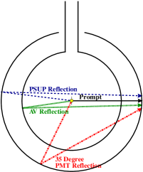
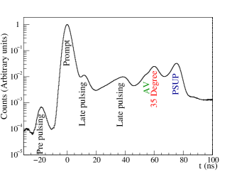
Figure 3: Top: Optical light paths within the detector. Bottom: PMT time residual distribution for laser data.

As with nearly all SNO calibration sources, the laserball can be deployed almost anywhere in two orthogonal planes within the acrylic vessel, as well as outside the vessel along a few vertical axes. For the data scans used to determine the optical parameters, we collected data four times with the laserball at the center and 18 times off-center at radii between 100 cm and 500 cm. Each of the central-position data collections was done with four different azimuthal orientations of the laserball, to help understand anisotropies in its light output. We kept the laser intensity relatively low (typically only about 5% of the PMTs registered hits for each laser pulse) so that the corrections that we applied to account for multiple photons hitting a single tube were small.

The optical model used to predict the number of prompt counts $N_{ij}$ observed in PMT $j$ in a given run $i$, within the $\pm 4$ ns window, is parameterized as follows:

$$N_{ij}=N_{i}\Omega_{ij}R_{ij}T_{ij}L_{ij}\varepsilon_{j}e^{-\left(d_{d}\alpha_{d}+d_{a}\alpha_{a}+d_{h}\alpha_{h}\right)}.$$ (2)

$N_{i}$ is a normalization parameter, proportional to the number of photons emitted by the laserball in run $i$ that can be detected within the prompt time window at each PMT. $\Omega_{ij}$ is the solid angle subtended by PMT $j$ with respect to the source position for run $i$. $R_{ij}$ is the PMT and concentrator assembly response aside from solid angle considerations, parameterized as function of the incidence angle on the PMT. $T_{ij}$ is the product of the Fresnel transmission coefficients for the heavy-water/acrylic/light-water interfaces. $L_{ij}$ is the laserball light intensity distribution, parameterized as a function of the polar and azimuthal angles of the light ray relative to the laserball center. The $\varepsilon_{j}$ are the relative PMT efficiencies for normally incident light, combining concentrator, PMT and electronics effects. $d_{d}$, $d_{a}$ and $d_{h}$ are the distances of the light paths through the D₂O, acrylic, and H₂O respectively. The $\alpha$s are the attenuation coefficients of the respective media, including the effects of both bulk absorption and Rayleigh scattering.

The parameters $\Omega_{ij}$, $T_{ij}$, $d_{a}$, $d_{d}$ and $d_{h}$ can be calculated from the source position and detector geometry, but the normalization $N_{i}$ and laserball intensity distribution $L_{ij}$ must be determined from the source data, together with the parameters required for the optical response model, $R_{ij}$, $\alpha_{d}$, and $\alpha_{h}$. The acrylic attenuation coefficient, $\alpha_{a}$, is fixed to ex-situ measurements performed as described in av . To take into account the probability of multiple photoelectron (MPE) hits, the number of prompt counts $N_{ij}$ is corrected by inverting the expected Poisson distribution of the hit counts,

$$N_{ij}^{MPE}=-N_{pulses}\ln(1-N_{ij}/N_{pulses}),$$ (3)

where $N_{pulses}$ is the total number of laser pulses in the run.

To remove the dependence on the imprecisely known PMT efficiencies $\varepsilon_{j}$, instead of $N_{ij}^{MPE}$ for each PMT we use an ‘occupancy ratio’ $O_{ij}$ of the MPE-corrected number of counts in PMT $j$ for run $i$ to the MPE-corrected number of counts for a run with the laserball in the center of the detector, $O_{0j}$.

The terms that can be calculated purely from source-PMT geometry are the solid angle $\Omega_{ij}$ and the product $T_{ij}$ of the Fresnel transmission coefficients. These two terms are used to correct the occupancy ratios measured with calibration data:

$$O^{data}_{ij}=\frac{N_{ij}^{MPE}}{N_{0j}^{MPE}}(\frac{\Omega_{0j}T_{0j}}{\Omega_{ij}T_{ij}})$$ (4)

The occupancy ratio calculated from the optical model is:

$$O^{model}_{ij}=\left(\frac{N_{i}^{MPE}}{N_{0}^{MPE}}\right)\frac{R_{ij}L_{ij}}{R_{0j}L_{0j}}e^{\delta d_{d}\alpha_{d}+\delta d_{a}\alpha_{a}+\delta d_{h}\alpha_{h}}$$ (5)

Here $\delta d_{x}=d_{ij}-d_{i0}$ is the difference in path length between run $i$ and a run with the laserball in the center for light traveling from the laserball to the $j$th PMT through each of the three modeled media (heavy water, acrylic, and light water) . We then derive the optical parameters by minimization of the $\chi^{2}$ between the data and the model:

$$\chi^{2}=\sum^{N_{runs}}_{i}\sum^{N_{PMT}}_{j}\frac{(O^{data}_{ij}-O^{model}_{ij})^{2}}{(\Delta O_{ij})^{2}+\sigma^{2}_{PMTij}}$$ (6)

The parameters over which $\chi^{2}$ is minimized are the attenuation coefficients, the average angular response $R_{ij}$ (assumed to be the same for every PMT) as a function of the incident angle of the light, the normalization constant $N_{i}$, and the laserball anisotropy $L$ as a function of solid angle. In Equation 6, $\Delta O_{ij}$ is the statistical uncertainty in the occupancy ratio due to counting statistics and $\sigma^{2}_{PMTij}$ is an additional uncertainty introduced to account for tube-by-tube variations in the PMT angular response as a function of the incidence angle of the light.

Figure 4 shows the D₂O attenuation lengths measured in SNO for two different data sets, compared to previous measurements and the Rayleigh scattering limit. We see that the SNO heavy water is the clearest large sample ever measured. Figure 5 shows the attenuation lengths for the light water surrounding the heavy water volume.

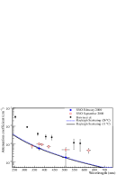
Figure 4: Measured D₂O attenuation lengths, compared to the data of Boivin et al. boivin .

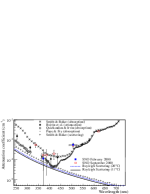
Figure 5: Measured H₂O attenuation lengths compared to the data of Smith and Baker smbaker , Boivin et al. boivin , Quickenden and Irvin quick , and Pope and Fry pope .

In addition to the attenuation lengths, minimization of the $\chi^{2}$ shown in Equation 6 also returns the response of the photomultiplier tubes and light concentrators as a function of incidence angle. The form of this response is one of the biggest sources of the position-dependence to the overall detector response.

Within the fit to the optical model, we parameterize the angular dependence as a simple binned response function, with 40 bins ranging from normal incidence to the highest angle possible from sources inside the heavy water volume (roughly $40^{\circ}$). Here, normal incidence is defined as normal to the front plane of the PMT and concentrator assembly (the face of the concentrator ‘bucket’), or, in other words, parallel to the PMT axis of symmetry. For the detector response used in the energy calibration (see Section V.5.2), it is this binned form which is used.

Within the Monte Carlo simulation, however, the Cherenkov photons are tracked through a complete three dimensional model of the PMT geometry. The model was based entirely on ex-situ measurements of the photocathode and concentrator assembly the:lay . By including the full geometry, the Monte Carlo model has the advantage that it correctly reproduces the timing of reflected photons, in particular the important ‘$35^{\circ}$ reflections’ shown in Fig. 3 that occur when a photon bounces off the photocathode and then the PMT concentrator the:moffat . These reflected photons ultimately affect the accuracy of event position reconstruction, which depends upon the timing of the PMT hits. Rather than using the optical fit of Equation 6 to extract all the microscopic parameters associated with the three dimensional PMT model, we created a hybrid model in which a small number of the three dimensional parameters were tuned in order to reproduce the binned angular response derived from the optical fit. These parameters altered the ex-situ-measured PMT photocathode efficiency as a function of radial distance from the PMT central axis. Light that strikes the concentrators at normal incidence (defined the same way as above) is reflected to the edge of the photocathode, and thus with the tuned photocathode efficiency the overall hit probability for these photons was reduced. Figure 6 shows the comparison between the resultant modeled response and the measurement. With the hybrid model, we correctly reproduce both the PMT timing and angular response, at the cost of a somewhat phenomenological (rather than an entirely physical) basis for the Monte Carlo model.

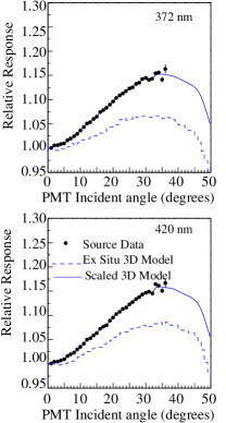
Figure 6: PMT angular response model compared to laser source data and to the hybrid model that adjusts the ex-situ measurements to agree with the data, for two wavelengths. Note that the zero has been suppressed.

We have studied the sensitivity of our optical measurements to laserball position uncertainties, data selection criteria, laserball isotropy and acrylic vessel position. The dominant systematic uncertainties associated with the optical parameters arise from uncertainties in the position of the laser source relative to the PMTs, and enter primarily through calculation of the PMT solid angle used in Equation 2. We estimated these uncertainties in several different ways, including making independent measurements of the positioning of the sources by touching the walls of the acrylic vessel, and timing the reflections of the laser light off the PMT array.

IV.8 Energy Scale

The calibrated optical parameters are used as input to the Monte Carlo model. The model accounts for photon scattering and absorption, tracking through the region of the PMT concentrators, to the PMT face, and ending with absorption in the photocathode and photoelectron emission. Electron optics in the PMT and subsequent charge collection and discrimination are not modeled, but an overall efficiency for these processes is included as a probability for a given photo-electron to produce a PMT hit. This probability is defined as

$$P_{hit}=\epsilon_{c}\epsilon_{t}$$ (7)

where $\epsilon_{c}$ is the efficiency for collecting photoelectrons produced at the photocathode onto the first PMT dynode ($\sim$ 70 %), and $\epsilon_{t}$ is the fraction of PMT pulses which generate a hit after passing through the electronics chain and discriminator (approximately 80% for 1/4 p.e. threshold), so that $P_{\rm hit}\approx 0.56$. $P_{\rm hit}$ thus sets the detector’s ‘energy scale’, and allows the model to correctly predict the number of detected PMT hits per MeV given an event’s location and direction. Phenomenologically, the determination of $P_{\rm hit}$ corresponds to determining the average quantum and detection efficiency of the PMT array, though in practice it includes other effects such as incompletely modeled optical responses and the efficiencies of the instrumentation.

As is described later in Section V.5, we used two estimators of an event’s energy: an estimation based on the raw number of total hits in the event (the ‘$N_{\rm hit}$’ estimator), and an estimation based on hits in a narrow $\pm 10$ ns time window, corrected for position- and direction-dependent effects (the energy ‘reconstructor’). The energy reconstructor was used to produce the initial Phase I results SNO Collaboration (2001, 2002a, 2002a), and the $N_{\rm hit}$ estimator, which has different sensitivities to systematic effects, was used as a verification check. The energy reconstructor’s $\pm 10$ ns window was chosen to be wider than the $\pm 4$ ns optical calibration prompt-time window to maximize the number of hits available for reconstruction, without needing to include significant corrections for scattered or reflected photons.

To determine the absolute energy scale for both estimators, we compared Cherenkov events from the ¹⁶N calibration source to Monte Carlo predictions of the detector’s response to the source. The code used to make the predictions simulated the production and emission of $\gamma$-rays, and included a model of the source geometry and optics. The state of the detector (for example, the average PMT noise rate and off-line or inoperative PMTs and electronics channels) at the time of the calibration run was taken into account.

$P_{\rm hit}$ is determined using ¹⁶N data with the source deployed at the detector center. For the energy reconstructor, we found the peak of the in-time hit distribution occured at 36.06 hits, for ¹⁶N runs taken mid-way through the D₂O phase. Based on this number, the value of $P_{\rm hit}$ which correctly scaled the Monte-Carlo was 0.566, a correction of approximately $5\%$ to the value of $P_{\rm hit}$ determined from ex-situ estimates of the PMT collection efficiency and hardware thresholds. The energy scale was sampled by many ¹⁶N calibration runs made throughout the running period. As shown in Fig. 14, we found a small energy scale drift which appeared to be caused by small changes in detector optics or PMT characteristics to which the optical calibration was not sensitive, such as the global PMT quantum efficiency. To correctly model the response as a function of time, we therefore applied a correction to event energy using a piecewise linear fit to Fig. 14 (described further in Section V.5). In the Monte Carlo model, we used a fixed energy scale for all simulations, set to reproduce data taken during the middle of the data acquisition period. Note that the absolute calibration of $P_{\rm hit}$ and the drift correction function are the only corrections applied to the simulation, after the inputs from the optical model.

IV.9 Electronics and Trigger

The Monte Carlo model includes many of the details of the detector instrumentation. We tracked the detector state run-by-run, saving in the SNO database information such as the number of electronics channels online, number of working PMTs, and number of working trigger signals. This information was fed into the Monte Carlo simulation, so that each data run was simulated with the correct detector configuration. Although the thresholds and gains of the individual PMTs were also tracked, we did not use this information to simulate individual PMT responses, but set all PMTs to the average (see Section IV.8).

The PMT noise rate was also tracked in every run using the pulsed trigger described in Section III. The average noise rate for each run is used in a simple Poisson model to add noise hits to the simulated events.

The PMT hit timing was simulated using test-bench timing measurements, and included a nearly Gaussian prompt peak whose width was 1.6 ns, as well as the pre-pulsing and latepulsing structure seen in Fig. 3. We simulated the PMT single photoelectron charge spectrum also using distributions drawn from test-bench measurements, with each PMT assumed to have the same gain. We did not simulate tube-by-tube efficiencies due to different PMT thresholds and gains.

An ‘event’ within the simulation is subject to the same trigger criterion as events in the SNO detector, using a model of the analog trigger signals themselves the:msn ; elec . Although the model can include the measured trigger efficiencies, the SNO trigger threshold is set so low and the trigger efficiency is so high that the difference between using a ‘perfect’ trigger and the true trigger efficiencies in the model was negligible. We therefore simulated events with perfect efficiency.

After an event is triggered in the simulation, the PMT times are calculated relative to the trigger time and stored along with the simulated PMT charges. We did not digitize the PMT times and charges in the simulation because studies of the effects of the digitization showed only negligible effects on the analysis. The final simulated data thus looked like calibrated PMT times and charges.

V Data Processing

In this section we describe the data processing used to calibrate, filter, and reconstruct the data set. As discussed in Section II and shown in Table 26, we created multiple distinct methods for all major analysis components. In the following we discuss the multiple methods used for identification and removal of instrumental backgrounds, position and direction reconstruction, and energy estimation. We leave the estimation of the numbers of residual background events to Section VII.

V.1 Raw Data

Each event recorded by the SNO detector contains several items of ‘header’ information: the trigger ID number, a word specifying which trigger or triggers fired in the event, the master clock time, and an absolute clock time synchronized to the GPS system. The GPS system provides time with resolution of 100 ns and an accuracy of $\sim 300$ ns. For each hit channel three digitized charges (a high gain, short integration-time charge; a high gain, long integration-time charge; and a low gain, long integration-time charge) and one time are recorded. All hit times are relative to the time-of-arrival of the global trigger.

V.2 Charge and Timing Calibrations

To convert the digitized charges and times to values that can be used in reconstruction and energy calibration, we subtracted pedestal values and converted the times from ADC counts to nanoseconds. The time conversion was done by linearly interpolating between 10 precisely measured pulser calibration times. The digital resolution for the times was approximately 0.1 ns, more than 10 times smaller than the intrinsic PMT time resolution. The charges were not converted into picocoulombs or photoelectrons, but left as pedestal-subtracted ADC count values.

The pedestals and timing slopes were measured twice weekly, and during data processing we applied the most recently measured set of calibrations. The pedestals were extremely stable—the variations from calibration to calibration were typically as small as could be measured (below one ADC count). The output of the pedestal and time calibration included quality control flags that we used to reject channels which were noticeably bad, or came from boards that had been replaced but not yet calibrated.

In addition to the pedestals and slopes applied to the digitized times, we also measured and subtracted the global channel-to-channel timing offsets (caused by differences in PMT transit times and small variations in signal path lengths) using data from the laserball source described in Section IV.7. The laserball data also provided us with a charge-dependent correction to the measured PMT times, necessary to account for the variation due to the risetime of the PMT pulses.

As was discussed in Section III, during the data acquisition period we discovered two problems with the charge and timing calibrations. The first problem was the slow development of non-linearities in the time- and charge-digitizing ADCs. Although we ultimately developed a hardware fix for the ADCs, for data taken before the fix was implemented we applied the quality control flags discussed above to reject affected channels.

The second problem was the small rate dependence of the time and charge pedestal values—the pedestal calibrations were typically taken at high rate while the actual neutrino data was low rate, and therefore the ‘true’ pedestal needed for the neutrino data could be a few counts different from the calibrated pedestal value. We developed a hardware solution to mitigate this problem, too, but also adjusted the time pedestal of each channel offline based upon the time since it last recorded a hit. This adjustment removed most of the problem, but for nearly all important calibrations (such as energy scale or the reconstruction of event position) we used radioactive source data taken at both high and low rates to ensure there were no residual effects. The rate dependence of the charge measurement was not corrected, but, as described later in Section V.5.2, the overall analysis was designed to depend only weakly on the charge measurement.

Figure 7 shows the width of the ‘prompt’ peak of the time residuals for the ¹⁶N calibration source deployed at the center of the detector. The 1.5 ns width is slightly better than what we had anticipated based on benchtop measurements.

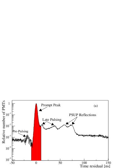
Figure 7: Time residual histograms from ¹⁶N calibration data at (a) center of the detector and (b) $r=500$ cm. The pre-pulsing and late pulsing peaks are properties of the PMTs and do not depend on the source position, while the reflection peaks from the PMT support sphere vary with source position. The shape and fraction of light in the main peak used for energy calibration (shaded) is reasonably insensitive to source position.

V.3 Instrumental Background Cuts

In addition to neutrino interactions, cosmic rays, and radioactive decays, the SNO detector also collects and records many background events produced by the detector instrumentation itself. They have several sources and span the energy range of interest for solar neutrino analysis. Although these events are relatively easy to distinguish from neutrino events, because of their much higher frequency a high rejection fraction is needed to ensure they do not contaminate the final data sample. More information on the instrumental backgrounds and the cuts used to remove them can be found in Appendix XV and Refs. the:mccauley ; fistdoc .

There are four distinct classes of instrumental background sources:

• Photomultiplier Tubes

  Small discharges within a PMT can produce detectable light. Although for a single PMT this occurs rarely (roughly once each week), integrated over the entire array we see roughly one such ‘flasher’ event each minute. Further, seismic activity within the mine—either natural or mining-related—can cause thousands of PMTs to flash within several tens of milliseconds.

  The PMTs can also produce light due to high voltage breakdown in their connectors or bases. Such events light up nearly the entire PMT array, and are accompanied by electronic pickup in neighboring electronic channels and crates.

• External Light

  Light outside the PMT array can generate detectable hits by entering through the neck region of the acrylic vessel or through the backs of the photomultiplier PMTs. For example, static discharges in the neck of the acrylic vessel, and at the boundary of the acrylic, nitrogen cover gas, and the water surface, can produce hits at the bottom of the PMT array.

• Electronic Pickup

  Activity near the electronics racks causing electronic noise can produce radiative pickup in many channels at once. Readout of a crate can occasionally produce hits confined to a single card in an electronics crate.

• Acrylic Backgrounds.

  The acrylic vessel itself sometimes emits isotropically distributed light at several locations; this light does not appear to be associated with any radioactivity.

To remove the vast majority of these events efficiently, we developed a suite of ‘low-level’ cuts which are applied to the data set before reconstruction (see Appendix XV). The cuts are based on information such as the distribution of PMT charge measurements, the total integrated charge, the time distribution of PMT hits, the inter-event timing, the spatial distribution of PMT hits, and the firing of veto PMTs installed in the neck region and outside the PMT support sphere. ‘Flasher’ events, for example, are characterized by a high charge in the offending PMT; electronic pickup events have many channels whose integrated charge is near the pedestal level. The cuts were designed individually as coarse filters to remove the most obvious background events, but the combination of the cuts removed nearly all the instrumental backgrounds (see Section VII.1) before the more sophisticated stages of the analysis. Figure 8 illustrates the removal of instrumental backgrounds from the raw PMT data as successive groups of cuts are applied. Each group of cuts primarily targets a different source of instrumental background. The figure also shows the effects of the high level (‘Cherenkov Box’) cuts described in Section V.6 and the fiducial volume cut which restricts events in the final signal sample to have a reconstructed radial position $R_{\rm fit}<550$ cm. We see that in the region of interest for solar neutrinos (40–120 hit PMTs) the cuts reduce the number of events in the data set by several orders of magnitude.

Figure 8: The reduction in the total number of events, as a function of the number of hit PMTs, for successive applications of the instrumental background cuts. In the figure, 1 MeV corresponds to roughly 8.5 hit PMTs.

Each of the cuts returns a simple binary decision. The results are saved as tags for each event, and the actual elimination of events based on the tags is done at the end of the analysis.

With such a large reduction in the number of events, we were particularly cautious in developing the cuts and measuring their signal acceptance. Nearly all the cuts were developed on a small subset of the total data set, primarily data taken during detector commissioning and the collection of radioactive source calibration data. Unbiased data sets containing instrumental backgrounds (such as bursts of flasher events caused by seismic activity) were also used in the creation of the cuts. We developed two separate sets of cuts, created by groups working independently, and performed extensive comparisons between them. Figure 9 compares the energy spectra (as measured by the number of hit PMTs) for a set of neutrino data that has been been subjected to both sets of cuts. As can be seen in the plot, the differences between the numbers of accepted events is extremely small, and our measurements showed that this difference is consistent with the difference in the signal acceptances of the two sets of cuts.

Figure 9: Comparison of the number of events remaining after application of the two separate sets of instrumental background cuts, as a function of the number of hit PMTs. As can be seen, the differences between the data sets are very minor.

As described in Section IX.3.1, the acceptance of signal events for the final suite of low-level cuts was measured to be greater than 99.5%.

V.4 Position and Direction Reconstruction

We use reconstructed position and direction both to produce the pdfs shown in Fig. 2 as well as to reject background events originating in the light water and PMTs. Further, as described in Section V.5, estimation of an event’s energy requires knowledge of its position and direction. We used two different position reconstruction algorithms. For the final analysis presented here and in our initial Phase I publications, we used one to provide the starting position and direction (the ‘seed’) for the other, thus ultimately obtaining a more accurate fit than either algorithm would have produced alone.

Both reconstruction algorithms use time-of-arrival of photons at the PMTs as the primary basis for determining event position. The algorithms treat photons as being created at a point at a single instant, and then calculate the arrival times using straight-path trajectories from the point source to a hit PMT. A likelihood is then calculated through comparison of the actual hit times to the hypothesized distribution of times. The second of the two algorithms also uses the angular distribution of PMT hits relative to an hypothesized electron direction. A likelihood is calculated by comparing the measured angular distribution of hits to the hypothesis that the event begins as a single 5 MeV Cherenkov electron.

The first step in the fitting procedure of the first algorithm is to search a coarse three-dimensional grid of 1.5 meter spacing across the entire detector volume. At each grid point a likelihood function is maximized with respect to time, the only remaining free parameter. The 20 grid points with the highest likelihoods are used as starting points for maximizing the same likelihood function, but this time in four parameters, $x,y,z,$ and $t$. The highest likelihood value found determines the best fit vertex gridfit .

The probability density function (pdf) used to calculate the likelihood in this stage of reconstruction depends solely on the PMT time-of-flight residuals $t^{\rm res}_{i}$ relative to the hypothesized fit vertex position. For the $i$th PMT, $t^{\rm res}_{i}$ is defined as

$$t^{\rm res}_{i}=t_{i}-t_{\rm e}-|\vec{r}_{\rm e}-\vec{r}_{i}|{n^{*}}/c$$ (8)

where $t_{i}$ is the hit time of the $i$th PMT, $t_{\rm e}$ is the time being fit, $\vec{r}_{\rm e}$ is the event position being fit and $\vec{r}_{i}$ is the PMT position. The photons are assumed to travel at a group velocity $c/{n^{*}}$ with ${n^{*}}$ an effective index of refraction averaged over the media in the detector. For this stage of the fitting, the pdf $P(t^{\rm res})$ was generated by Monte Carlo simulation of low energy background events in the light water region. The fit for vertex position and time amounts to shifting $\vec{r}_{\rm e}$ and $t_{\rm e}$ until the largest number of PMT hit times lie underneath the peak of the in-time distribution. The logarithm of the likelihood function used to do the fit at this stage is:

$${\log\cal L}=\Sigma_{i=1}^{\rm N_{\rm hit}}\log(P(t^{\rm res}_{i})).$$ (9)

Once the vertex location has been determined, the direction is fit by a maximum likelihood method based on a pdf of the angular distribution of photons relative to the initial direction of a simulated 5 MeV electron.

The vertex and direction obtained thus far are passed to the second reconstruction algorithm which differs primarily in that it simultaneously fits the event position, time, and direction using both timing and angular information. The log-likelihood function maximized as a function of $\vec{r}_{e}$, $t_{e}$, and $\vec{v}_{e}$ is:

$${\log\cal L}=\sum_{i=1}^{N_{hit}}\log{\cal P}(\vec{r}_{e},\vec{v}_{e},t_{e};t_{i},\vec{r}_{i})$$ (10)

where $t_{i}$ is the measured PMT hit time and $\vec{r}_{i}$ is the PMT position; $\vec{r}_{e}$ is the event vertex, $\vec{v}_{e}$ is the event direction, and $t_{e}$ is the event time. As before, the angular part of the pdf is based on the assumption that the event begins as a single Cherenkov electron.

The probability ${\cal P}$ contains two terms, to allow for the possibilities that the detected photon arrives directly from the event vertex (${\cal P}_{\rm direct}$), or results from reflections, scattering, or random PMT noise (${\cal P}_{\rm other}$). These probabilities are weighted based on data collected in the laserball calibration runs: ${\cal P}=f_{\rm direct}{\cal P}_{\rm direct}+f_{\rm other}{\cal P}_{\rm other}$, with $f_{\rm direct}=0.879$, and $f_{\rm other}=0.121$.

${\cal P_{\rm direct}}$ and ${\cal P_{\rm other}}$ are further broken down into separate time and angle factors:${\cal P_{\rm direct}=P^{\rm TIM}P^{\rm ANG}}$, for example. The time factor was based on the time residual distributions determined from the laserball calibration data with the source at the center of the detector. (The time residual is defined in Equation 8). We characterized the direct light time distribution with a sum of four Gaussians corresponding to prompt, pre-pulse, late-pulse and after-pulse PMT hits. Non-direct light was characterized by a step function with the value for $t^{\rm res}<0$ corresponding to random PMT noise, and for $t^{\rm res}>0$ corresponding to random noise plus an average contribution from reflected and scattered light. Figure 10 displays the PMT time distribution from the laser calibration data along with the functions used to describe the distribution.

The angle factor is the Poisson probability for a single photon hit in a PMT.

$${\cal P}^{\rm ANG}=N_{\gamma}\rho_{i}e^{-N_{\gamma}\rho_{i}}$$ (11)

where $N_{\gamma}=N_{\rm hits}/P_{hit}\equiv N_{\rm hits}/0.55$ is an estimate of the number of photons which strike PMTs (see Equation 7) and

$$\rho_{i}=\frac{1}{2\pi}g(\cos\alpha_{i})\Omega_{i}$$ (12)

where $g(\cos\alpha)$ is the angular distribution of the photons relative to the initial electron direction, $\alpha_{i}$ is the angle of the $i$th PMT relative to the hypothesized electron direction as measured from the vertex, and $\Omega_{i}$ is the solid angle of the $i$th PMT as viewed from the vertex:

$$\Omega_{i}=\frac{\pi r_{c}^{2}}{d_{i}^{2}}\hat{d}_{i}\cdot\hat{r}_{i}.$$ (13)

In Equation 13, $r_{c}$ is the radius of the PMT concentrator ‘bucket’ (see Section IV.7), $\vec{d}_{i}$ is the vector from the event vertex to the center of the face of the concentrator bucket, and $\vec{r}_{i}$ is the position of the front face of the PMT in detector coordinates.

Figure 11 shows the angular distribution assumed for the direct photons. The non-direct photons are assumed to be isotropic relative to the event vertex and hence to have a flat distribution in $\cos\alpha$.

The azimuthal symmetry of Cherenkov light about the event direction dilutes the precision of reconstruction along the event direction. Scattering of photons out of the Cherenkov cone thus systematically tends to drive the reconstructed event vertex downstream of the true event position. To compensate for the systematic drive, after initial estimates of position and direction are obtained, a correction is applied to shift the vertex back along the direction of the event, varying with the distance of the event from the PMT sphere as measured along its direction.

In the final stage of the fit, the hypothesis that the event was a single electron is tested. We do this using two figure-of-merit criteria calculated from the angular distribution of the PMT hits relative to the event vertex and direction. The first of these is a Kolmogorov-Smirnov test of the uniformity of the azimuthal distribution of PMT hits around the event direction. The second is a two-dimensional Kolmogorov-Smirnov test of the distribution of hit PMT directions azimuthally and in $\cos{\alpha}$ relative to the reconstructed event direction.

Figure 10: A plot of the distribution of PMT hit times from a laser calibration run. Overlaid on the data are the pdfs used in the fitter to characterize the direct light (dashed) and the pdf describing the non-direct light (dotted). The summed pdf is also displayed (solid line). As only the relative times of the PMT hits are relevant in the event reconstruction, the offset of the “prompt” peak from zero is unimportant.

Figure 11: Parameterized angular distribution of Cherenkov photons relative to the initial direction of a Monte Carlo 5 MeV electron. This distribution is used as the pdf for the direct PMT hits in reconstruction.

Figure 12 shows the $x$-coordinate resolution of vertex reconstruction for events for a Monte Carlo simulated sample of CC electrons. The performance of the reconstruction algorithm on data and its associated uncertainties will be presented in Section VI.1.

Figure 12: The distribution of the difference between the reconstructed $x$ position ($x_{\rm fit}$) and the true position $x_{\rm true}$ for a sample of Monte Carlo simulated CC electrons.

V.5 Energy Calibration

We used two different estimators of event energy as assurance against unexpected systematic errors. One was simply the total number of hit PMTs (‘$N_{\rm hit}$’), without any adjustment for the position dependence of the energy scale within the detector. For this estimator, the energy spectra in the top row of Fig. 2 were replaced by ‘$N_{\rm hit}$ spectra’. The second estimator, the energy ‘reconstructor’, used the fitted event position and direction and the analytical form of the optical model described in Section IV.7. The energy reconstructor was used to produce the results reported in the intial Phase I publications, and the $N_{\rm hit}$ estimator used for validation of those results. In this section, we briefly discuss the $N_{\rm hit}$ estimator (for more details, see Refs. the:msn ; the:kh ; the:pw ) and give a more complete description of the energy reconstructor.

V.5.1 ‘$N_{\rm hit}$’ Energy Estimator

Using the total number of hit PMTs in an event ($N_{\rm hit}$) as an energy estimator has the advantage that it is simple: it uses no cuts on charge or time to define good and bad hits, it integrates over uncertainties in the time distribution of reflected and scattered light, and it applies no corrections to the data itself. Also, the additional statistics gained by including scattered and reflected light can lead to a narrower energy resolution overall. Although the calibrations of our optical model have explicitly been done only for prompt light (see Section IV.7), as Fig. 7 shows the fraction of late light in an event is only $\sim$12%. We can therefore include reflected and scattered light even if our knowledge of the optical parameters which govern its generation and propagation are somewhat worse than for direct light. Most importantly, the use of total $N_{\rm hit}$ is sensitive to different systematic effects from the prompt-light energy reconstructor described in the next section.

To use total $N_{\rm hit}$ to extract signal fluxes, we employ the Monte Carlo simulation to generate pdfs like those shown in Fig. 2, with the top row replaced by $N_{\rm hit}$ spectra. With the data untouched by any correction or calibration, one must ensure that the Monte Carlo simulation takes into account the variations in detector state over the data collection livetime. For example, the number of working channels as a function of time and the change in PMT noise rates must be tracked and fed either into the Monte Carlo simulation (as described in Section IV.9) or applied as subsequent corrections.

The only calibration necessary here is therefore that described in Section IV.8—the initial calibration of the Monte Carlo model to ensure that the predicted number of hits per event agrees with the measurements using sources. The uncertainty of this calibration will be discussed in Section VI.2. Figure 13 shows a comparison of the Monte Carlo model’s prediction of the distribution of $N_{\rm hit}$ for the ¹⁶N source to an actual source run.

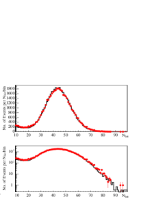
Figure 13: $N_{\rm hit}$ distributions for Data (dots) and Monte Carlo simulation (line) for a ¹⁶N calibration at the detector center, on both linear and logarithmic scales.

V.5.2 Energy Reconstructor

Unlike the ‘$N_{\rm hit}$’ energy estimator, the energy reconstructor corrects for detector optical, temporal, and spatial effects to assign a most probable energy to each event. Given an event’s position, direction, and number of hit PMTs, the energy reconstructor uses the analytic form of the optical model described in Section IV.7 to estimate the number of PMT hits the event would have produced had it been created at the center of the detector. A scale factor is then applied to convert the number of hits to an equivalent electron energy.

This reconstruction has several advantages over the simple ‘$N_{\rm hit}$’ estimation. First, it allows us to produce energy spectra labeled in MeV, rather than the detector-specific $N_{\rm hit}$. Also, by correcting for the detector’s point-to-point variation in response we can choose to use a single analytic function to map true energy to reconstructed energy, rather than relying on the entire Monte Carlo model to provide the detector response. With such an analytic function, we and others wishing to fit our data set can create pdfs in energy which do not require the entire detector simulation.

As described in Section IV.7, measuring the optical parameters that characterize late hits, such as the degree of scattering and various reflection coefficients, can be difficult. In addition, in a particular event, there is no way to uniquely determine the flight paths of such out-of-time photons. The energy reconstructor therefore begins by eliminating out-of-time hits, restricting PMT times to be within $\pm$10 ns of the prompt time peak. The remaining hits are treated as if they came directly from the reconstructed event vertex. The $\pm 10$ ns window is applied to the PMT time residuals defined by:

$$t_{\rm res}=t_{\rm pmt}-t_{\rm fit}-t_{\rm travel}-t_{\rm shift},$$ (14)

where

$$t_{\rm pmt} =$$ calibrated PMT hit time

$$t_{\rm fit} =$$ fitted event time

$$t_{\rm travel} =$$ travel time from vertex to PMT

$$t_{\rm shift} =$$ average risetime correction shift.

$t_{\rm shift}$ is necessary because, as described in Section V.2, we discovered rate dependencies to the charge and time pedestal values. Although the effect was small, it meant that the measured PMT times, which nominally were corrected for PMT pulse risetime based on the integrated event charge, could vary as a function of event rate. By removing the risetime correction from the energy calibration, this variation was no longer an important source of systematic uncertainty, and with the prompt time cut used here, the loss of PMT timing precision is not critical. The value of $t_{\rm shift}$ was picked to center the uncorrected PMT timing residuals at $t_{\rm res}=0$.

Time residual histograms for ¹⁶N source runs at radii of $0.0$ cm and $500$ cm are shown in Fig. 7. One can clearly see the effects of scattering at the higher radius. The PMT reflection peaks, which are more than 50 ns from the prompt peak with the source at the center, move closer as the source is moved toward the PMT array.

With the ‘prompt’ PMTs in an event identified, we define an effective number of PMTs hit as

$$N_{\rm eff}=N_{\rm win}-N_{\rm dark}$$

with

$$N_{\rm win} = \pm 10$$ number of in-time hits ( ns)

and

$$N_{\rm dark} =$$ expected number of in-time noise hits.

The average number of PMT noise hits, measured using the pulsed trigger described in Section I, was found to be 2.1 in the 440 ns event timing window. (This is equivalent to an average dark noise rate for each photomultiplier tube of $\sim$ 593 Hz). Since the dark noise hits are uniformly distributed throughout the 440 ns window, the expected number of noise hits $N_{\rm dark}$ within the energy reconstructor’s 20 ns timing window is just 0.1. This number is small enough (equivalent to roughly 10 keV) that accounting for variations from run-to-run would have had a negligible impact.

We then apply optical and gain corrections to determine the equivalent $N_{\rm eff}$ at the detector center to produce a ‘corrected $N_{\rm hit}$’:

$$N_{\rm cor}=N_{\rm eff}\times\frac{1}{\epsilon_{\rm response}/\epsilon_{0}}\times\frac{1}{\epsilon_{\rm hardware}}\times\frac{1}{\epsilon_{\rm drift}}.$$ (15)

In Equation 15, $\epsilon_{0}$ is the detector’s optical response for an event at the detector center, and $\epsilon_{\rm response}$ represents the detector’s optical response for events at a given position ($\vec{r}$) and direction ($\vec{u}$):

$$\epsilon_{\rm response} =\sum_{\theta^{\prime}}\sum_{\phi^{\prime}}\sum_{\lambda}\frac{\epsilon_{\rm PMT}(\lambda)}{\lambda^{2}}g(\theta^{\prime},\phi^{\prime})$$ (16)

$$\times e^{-\mu_{1}d_{1}-\mu_{2}d_{2}-\mu_{3}d_{3}}R(\theta^{\prime},\phi^{\prime})M(r,\theta^{\prime},\phi^{\prime})$$

In Equation 16, the sums are over 10 polar ($\theta^{\prime}$) and 10 azimuthal ($\phi^{\prime}$) angle bins relative to the reconstructed event vertex and direction ($\theta^{\prime}$=0), and wavelengths $\lambda$ in a range (220-710 nm) that span the wavelengths to which the detector is sensitive. The factor $\epsilon_{\rm PMT}(\lambda)$ represents the efficiency of the PMT as a function of wavelength, and $g(\theta^{\prime},\phi^{\prime})$ is the angular distribution of Cherenkov light about the event direction. The $\mu_{i}$ are the inverse of the wavelength-dependent attenuation lengths for each medium ($i=1,2,3$ corresponding to D₂O, acrylic, and H₂O), and the $d_{i}$ are the distances through each medium that photons travel from the event vertex to the PMT array in each ($\theta^{\prime}$,$\phi^{\prime}$) bin. $R(\theta^{\prime},\phi^{\prime})$ is the PMT angular response, and $M(r,\theta,\theta^{\prime},\phi^{\prime})$ is a correction for the multiple hit probability (which depends on the event position, $r$). The largest variation in $\epsilon_{\rm response}$ within the D₂O as a function of source radius is about 7%, with its largest values occurring near $R=450$ cm.

The efficiency $\epsilon_{\rm hardware}$ is applied to correct for the number of PMTs available in a given event, which is tracked run-by-run and logged in the SNO analysis database. In addition, PMTs which are known to have poor response are flagged during the PMT calibrations described in Section V.2; their effect is then included as a reduction in $\epsilon_{\rm hardware}$.

We apply $\epsilon_{\rm drift}$ only to data (not Monte Carlo events), and we use it to correct for small changes in the overall photon collection efficiency of the detector over time. Figure 14 shows the time-dependent behavior of $N_{\rm eff}^{\prime}$, defined by

$$N_{\rm eff}^{\prime}=N_{\rm eff}\times\frac{1}{\epsilon_{\rm hardware}},$$ (17)

and we can see that, as discussed in Section IV.8, there was a drop in overall detector gain of about $1.8\%$ during the first several months of production running followed by slower drop for the remainder of the running period. The dashed line in Fig. 14 is used as a correction to the energy scale as a function of date, and is given by

$$\epsilon_{\rm drift} = 1.595-[6.315\times 10^{-5}\times{\rm JDY}]$$

for JDY $$<$$ 9356

$$= 1.004-[9.170\times 10^{-6}\times({\rm JDY}-9356)]$$

for JDY $$\geq$$ 9356

where JDY is ‘SNO Julian Date’. SNO Julian Day 9356 corresponds to midnight UTC, on August 12, 2000. As Section IV.8 describes, the Monte Carlo model’s energy scale was left fixed to the level determined in the middle of the data acquisition period, and so no $\epsilon_{\rm drift}$ correction is applied to simulated events.

Figure  15 shows the fractional deviation of the mean $N_{\rm win}$ after applying the drift correction. The mean deviation of this value from zero is about 0.25% which is consistent with statistical variation.

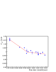
Figure 14: Photon collection efficiency ($P_{\rm hit}$) versus time. Shown is the value of the peak of the $N_{\rm eff}^{\prime}$ distribution from ¹⁶N calibration runs at the detector center, relative to the average over the data set. The dashed line is used as $\epsilon_{\rm drift}$, the correction to the absolute energy scale.

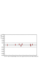
Figure 15: Fractional deviation of mean $N_{\rm win}$ for ¹⁶N source calibration runs after drift correction applied. Only a subset of the data in Fig. 14 is shown.

To map the corrected number of hit PMTs ($N_{\rm cor}$) to electron energy, sets of Monte Carlo calculations are performed for mono-energetic electrons at the detector center, at different electron energies. For each electron energy, we fit a Gaussian to the resultant $N_{\rm eff}$ spectrum to obtain a mean value. This is done for event energies covering our region of interest for solar neutrino analysis, from about 2-30 MeV, resulting in a linear relationship between $N_{\rm eff}$ and energy in MeV.

Using Monte Carlo events we calculate $N_{\rm cor}$ from Eq. 15 and use the generated linear map to produce a calibrated energy spectrum. For reference, Table  1 shows the predicted $E_{\rm eff}=T_{\rm eff}+0.511{~{}\rm MeV}$ peaks for various calibration sources.

Source	Peak $E_{\rm eff}$ [MeV]
16N	$5.486$
pT	$19.2$
n(d,t)$\gamma$	$5.59$

Table 1: Predicted $E_{\rm eff}$ peaks for calibration sources.

Figure  16 shows the $E_{\rm eff}$ spectra for ¹⁶N data and Monte Carlo, showing good agreement between energies in the region of interest for the solar neutrino analysis ($T_{\rm eff}>5$ MeV).

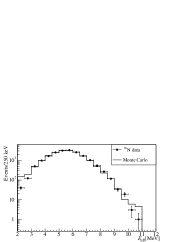
Figure 16: ¹⁶N $E_{\rm eff}$ spectra for calibration data and a Monte Carlo calculation, for a deployment near the center of the detector.

V.6 ‘Cherenkov Box’ Cuts

Although the ‘low-level’ instrumental background cuts described in Section V.3 are very efficient at removing backgrounds with specific characteristics (high charge in one or more PMTs, poor timing distributions, etc.) we still want to ensure that the final data set contains no events which are inconsistent with Cherenkov light. The defining characteristics of Cherenkov light are that it has a very narrow time distribution, and a hit pattern consistent with a Cherenkov cone. We therefore formulated two cuts, one based on timing and the other on hit pattern, which define a ‘Cherenkov box’ in which we expect only neutrino events and background events due to radioactivity to lie. These cuts used derived information—such as the reconstructed position of each event—as opposed to the low-level information used in the cuts described in Section V.3 and Appendix XV. We therefore refer to them as ‘high-level’ cuts.

Our measure of Cherenkov timing is simply the ratio of in-time hits to the total number of hits in an event, where ‘in-time’ is defined using reconstructed time-of-flight residuals like those of Equation 14. Unlike in Eq. 14, however, here we use the risetime-corrected hit times. The in-time window for this ratio is $-2.5\rightarrow+5.0$ ns relative to the prompt timing peak, and we restrict neutrino candidate events to have an in-time ratio (ITR) $>0.55$.

For the hit pattern cut, we reject events for which the mean angle between all pair-wise combinations of hit PMTs ($\theta_{ij}$) is either too large ($>1.45$ radians) or too small ($<0.75$ radians). The PMT pair angles are calculated as viewed from the reconstructed event vertex, and only PMTs within a small time window (within $\sim\pm 9$ ns of the prompt peak) are used. Events with mean pair angles greater than 1.45 radians are ‘too isotropic’ to be Cherenkov light; those with pair angles below 0.75 radians are ‘too narrow’ compared to a Cherenkov ring.

Figure 17 shows events plotted in these two characteristics. In black are events which have been tagged by the low-level instrumental background cuts, in grey are neutrino candidate events, and in blue are events from the ¹⁶N calibration source. As we see, most of the candidate events lie within the same Cherenkov box as do the ¹⁶N calibration source events. In fact, many candidate events which lie outside are mis-reconstructed events rather than instrumental backgrounds, as determined by calibration source data.

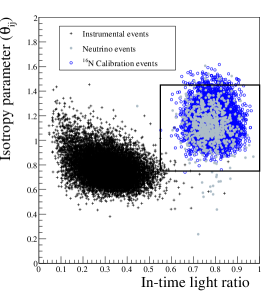
Figure 17: Fraction of in-time light for an event versus its mean PMT pair angle ($\theta_{ij}$). Events which pass the low-level cuts (grey) and those which fail (black) plotted on the high-level cut axes. ¹⁶N calibration source events are plotted in blue.

V.7 Muon and Atmospheric Neutrino Follower Cuts

While the rates in SNO of muons and atmospheric neutrino interactions are just 3 per hour, their products can be a dangerous source of background. Spallation by cosmic ray muons produces neutrons as well as long-lived radioisotopes. Atmospheric neutrino interactions can also produce neutrons, through both neutral current and charged current processes.

We remove cosmic-ray-muon spallation products by cutting all events occurring within 20 s of a muon event. The muon identification criteria require more than five hits in the outward-looking veto PMTs and more than 150 hits in inward-looking PMTs. To avoid large detector deadtime from this cut, we do not impose a deadtime following an event which satisfies these criteria but is also tagged by the low-level cuts as arising from a discharge in the neck of the acrylic vessel.

To remove the products of atmospheric neutrinos and muons missed by the muon tag, we also cut all events within a 250 ms interval following any event that has more than 60 PMT hits. This cut removed 53 events from the final neutrino candidate sample. In Section VII.6.2 we describe our estimate of the number of background events in the final data set passed by these cuts, and in Section IX.1 the associated livetime loss.

V.8 Fiducial Volume and Energy Threshold

The last set of cuts applied to the data set are intended primarily to remove backgrounds associated with low energy radioactivity within the detector. Radioactive decays within the heavy water volume typically produce much lower energy events ($\sim 2$ MeV) than interactions by the ⁸B solar neutrinos (up to 15 MeV), and we therefore remove the vast majority of backgrounds by imposing an energy threshold of $T_{\rm eff}=E_{\rm eff}-0.511~{}{\rm MeV}>5.0$ MeV.

Events originating from radioactivity in the regions outside the heavy water—from the light water shield, the acrylic vessel, the PMTs and associated support structure or the cavity walls—can remain in the final data sample only if they are both above the energy threshold and have misreconstructed positions. Nevertheless, these regions have far higher radioactivity levels than the D₂O (see Sections VII.2 and VII.4.2), and we therefore restrict the fiducial volume of the final sample to avoid these backgrounds. Our requirement that the final events reconstruct within 550 cm of the detector center also has the advantage that backgrounds from misreconstruction of light produced by the acrylic vessel are minimal (see Section V.3). Further, our understanding of the detector optics and response is best within the 550 cm fiducial volume.

Figure 18 shows a $z$ vs. $y$ projection for events above a threshold of $T_{\rm eff}=5.0$ that pass all cuts except the fiducial volume restriction. The fiducial volume used in this analysis indicated by the red line. As can be seen in the figure, there is a region of higher activity, a ‘hot spot’, near $z=450$ cm and $y=400$ cm. Although the origin of this hot spot is unknown, the characteristics of events which reconstruct there are consistent with decays in the natural radioactive chains. We discuss the hot spot as a source of background in Section VII.2.4 and as an in-situ ‘calibration’ source in Section XI.3.2.

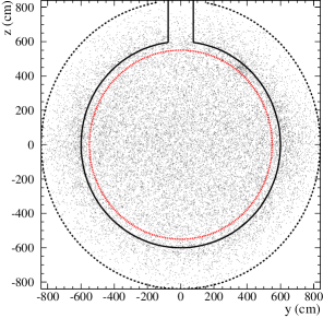
Figure 18: Projection of reconstructed positions of events within the SNO detector onto the $z$-$y$ plane, for an energy threshold of $T_{\rm eff}>5.0$ MeV. The dashed line shows the radius of the PMT support sphere (PSUP), the solid line the acrylic vessel, and the dotted line the fiducial volume cut used by SNO.

V.9 Data Processing Cut Summary

Table 2 details the number of events remaining after each cut applied during data processing.

Table 2: Number of events remaining in data set after each step in the data processing described in Section V.

.

Data Processing Step	Events Remaining
Total event triggers	450188649
Neutrino triggers (hit multiplicity)	191312560
Analysis $N_{\rm hit}$ cut ($N_{\rm hit}>21$)	10088842
Low-level cuts	7805238
‘Cherenkov Box’ cuts	3418439
Fiducial volume cut	67343
Energy threshold ($T_{\rm eff}>5$ MeV)	3440
Muon follower cut	2981
Atmospheric $\nu$ followers	2928
Total $\nu$ candidates	2928

VI Systematic Uncertainties on the Model

The pdfs shown in Fig. 2, created by the model described in Section IV, represent our best estimates of the true distributions of neutrino event energies, directions, and radial positions. Before we fit the processed data set, we need to evaluate the uncertainties on the pdf shapes. We rely on the model to generate the pdfs, rather than on calibration source data, because the sources themselves do not identically reproduce the neutrino signal data. Calibration source events differ from neutrino events in many ways: the source and deployment hardware affect the detected energy; sources like ¹⁶N are $\gamma$ sources but the detected products of the CC and ES reactions are electrons; the calibrations were performed at discrete points in the detector, while the neutrino events occur throughout the volume; and the calibrations were done at particular times while the neutrino data is distributed over the entire data acquisition livetime. As described in Section IV, the only two direct inputs to the model from the calibration source data are the optical properties of the detector and the overall energy scale.

What the calibration source data do give us is a powerful way of determining the systematic uncertainties on the model predictions of detector response. Rather than determining these uncertainties by varying (and covarying) each of the relevant parameters in the model (such as optical attenuation lengths or PMT efficiencies), we made direct comparisons of source data to model predictions of the response for each source. The differences between the model predictions and the source data were then used as estimates of the systematic uncertainty on the model’s ability to reproduce the detector behavior. As explained later in Section VIII, we determine the effects of these uncertainties on the neutrino flux measurements by varying the pdfs of Fig. 2 by amounts consistent with the uncertainties, and then re-fitting for the fluxes.

SNO’s extensive array of calibration sources and the ability to place them at many positions within the detector allowed us to explore the dependence of the uncertainties on nearly every way in which the simulation and the calibration data differed. Different source types allowed checks of the dependence on particle species, particle energies, and calibration-source apparatus; position dependence was provided by scans of sources throughout two orthogonal detector planes; rate dependence was explored by varying calibration source rate; time dependence was determined through periodic deployments of sources throughout the data acquisition period.

In addition to the Monte Carlo model, we also developed a set of analytic pdfs that described the response of the detector and used them to do a similar signal extraction (see Section VIII). The determination of the systematic uncertainties for the analytic pdfs were derived from direct fits to the calibration source data.

We describe below our determination of the uncertainties on the pdf shapes through model-data comparisons. Systematic uncertainties affecting the overall normalization of the fluxes such as those associated with livetime, knowledge of the Earth’s orbital eccentricity, and uncertainties on the acceptance of the cuts applied to the data set, are presented in Section X.

VI.1 Position and Direction Reconstruction

As discussed in Section V.4, we compared the results of two separate reconstruction algorithms to verify their performance. Ultimately, one algorithm, which used PMT timing information alone, was used to provide the ‘seed vertex’ for the second algorithm, which simultaneously fits event position and direction using both the timing and angular distribution of the hit PMTs. As there was not a significant difference in the uncertainties of the two algorithms, we describe below how the uncertainties were estimated for the final hybrid method.

The algorithm characteristics for which we need to determine uncertainties fall into three classes:

• Vertex Accuracy: The average distance between the true interaction position (in $x$, $y$, and $z$) and the reconstructed position. Many effects that can produce a systematic shift (such as a shift along the event direction due to the azimuthal symmetry of Cherenkov light) are already accounted for in the model, and what we are interested in here is the uncertainty on the model’s prediction of these shifts.

• Vertex Resolution: The width of the distribution of reconstructed event positions relative to their true positions. The resolution itself is well-modeled, but we need to determine the uncertainty on the model prediction.

• Angular Resolution: The distribution of reconstructed directions relative to the initial electron direction.

Ultimately, reconstruction uncertainties affect our flux measurement uncertainty in two ways. First, we need to know the uncertainty in our prediction of geometric acceptance—how many events we expect to reconstruct inside our fiducial volume. This acceptance uncertainty depends both on uncertainty in vertex resolution (if, say, the true resolution is broader or narrower than we believe, then we will over- or underestimate the number of events) and upon the possibility of systematic shifts in the mean fit position (outward or inward, upward or downward, etc.).

The second way in which these uncertainties affect our final answer is in the shapes of the pdfs we use for signal extraction. An error in the response function used to model the detector (either through Monte Carlo simulation or with an analytical model) will alter the number of events derived from our fits to the data. For this, reconstruction of both direction and position is important.

VI.1.1 Vertex Accuracy

A systematic shift inward or outward in mean reconstructed position is the most dangerous of the reconstruction-related uncertainties. Such a shift effectively shrinks or grows the fiducial volume. A +1% uncertainty in scaling on the radial coordinate, for example, produces a 3% uncertainty in the number of accepted events within the fiducial volume.

In estimating the uncertainty in vertex accuracy, we examine both $\rm{}^{16}{N}$ and $\rm{}^{8}{Li}$ data. We take our primary estimate of the uncertainty from the $\rm{}^{16}{N}$ data, and check for effects which depend on event energy or source type with the $\rm{}^{8}{Li}$ data. Both sources generate electrons with known position distributions (in the case of the $\rm{}^{16}{N}$ source, the electron position distribution includes the effects of Compton scattering by the $\gamma$ ray). To estimate the shift in the mean reconstructed vertex and the width of the resolution function, we convolve these known position distributions with a hypothetical resolution function, and then fit the resultant convolution to the data by allowing the mean and width of the resolution function to vary the:mgb ; the:msn . That is, a function $\xi(x_{fit};\sigma,\mu)$ is fit to the one-dimensional reconstructed position distribution (here shown in $x$),

$$\xi(x_{fit};\sigma,\mu)=\int\limits_{-\infty}^{\infty}F(x_{fit},\sigma,\mu;x_{src})S(x_{src})dx_{src}$$ (20)

where $S$ is the electron source distribution and $F$ is the reconstruction resolution function for electrons. $F$ includes both the width of the resolution ($\sigma$) and a shift in the mean ($\mu$). The one-dimensional form chosen for $F$ is a simple Gaussian,

$$F(x_{fit},\sigma,\mu;x_{src})=\frac{1}{\sqrt{2\pi}\sigma}e^{-\frac{[(x_{fit}-x_{src})-\mu]^{2}}{2\sigma^{2}}}$$ (21)

motivated by Monte Carlo studies of reconstructed electron position distributions.

Although a better fit to the Monte Carlo distributions is obtained using the sum of a Gaussian and an exponential (the data suggest exponential rather than Gaussian tails the:mgb ), for signal extraction using Monte Carlo signal pdfs we need only the Gaussian, since we are just trying to characterize differences between Monte Carlo distributions and calibration data distributions. As described above, in signal extraction we use these differences to evaluate the systematic uncertainties on the fitted event rates by convolving the Monte Carlo generated pdfs with smearing functions designed to broaden and shift the Monte Carlo simulated position distributions so that they look like those we have obtained with the data. In other words, we fit for the function $F$ for both Monte Carlo simulation and calibration data, and then find the Gaussian which smears the Monte Carlo-derived $F$ to yield the $F$ we measure for the data. This ‘smearing’ Gaussian is then convolved with the Monte Carlo-generated signal position pdfs (the second row of Fig. 2) and the signal extraction procedure repeated. The resultant change in the fiducial volume and the number of extracted neutrino events yields the uncertainty on the neutrino fluxes.

For our secondary signal extraction method (using analytical pdfs), one needs to include the exponential tails. In this case, the goal is to produce pdfs by convolving the expected true position distribution for events inside the detector volume with a resolution function derived primarily from data. To correctly reproduce the event position distributions without using the Monte Carlo model, the more complete distribution is therefore needed.

For $\rm{}^{16}{N}$, the form of $S(x_{src})$ is the one-dimensional projection of the three-dimensional Compton scattering distribution, $S(r)\sim\exp^{\frac{-r}{\lambda}}/r^{2}$, with $\lambda=37$ cm. The $\rm{}^{8}{Li}$ source is approximated as a source of electrons on a shell 10.7 cm in diameter.

The derived values of $\sigma$ and $\mu$ in our resolution function $F$ are in general functions of position, energy, and source type. We look first at position dependence. The comparison between Monte Carlo simulation and source data is done by first deriving the mean fit position as described above and comparing it to the measured source position, based on the information from the source-positioning mechanism. The precision of the source-positioning is the limit to our overall uncertainty, and hence the primary measurements of position-dependent shifts are done using scans along the $z$-axis, where the source position uncertainty is expected to be smallest ($\sim$2 cm). Figure 19 compares the mean reconstructed vertex for an $\rm{}^{16}{N}$ $z$-axis scan taken in October 2000 to results from a Monte Carlo simulation of the same scan.

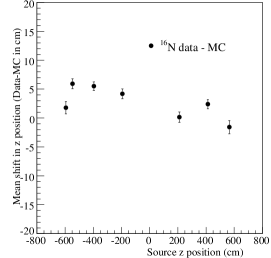
Figure 19: Difference between $\rm{}^{16}{N}$ source data and $\rm{}^{16}{N}$ Monte Carlo simulations of the vertex accuracy, using a precision $z$-axis source scan. Vertex accuracy is defined here as the difference between expected source position (based on the measurements by the source-positioning mechanism for data and the true source position for Monte Carlo simulated events) and reconstructed position. The shift between the Monte Carlo prediction and the data are consistent with a model that scales each event’s reconstructed radial position by $\pm$1%.

One approach to assigning a systematic uncertainty on the vertex accuracy based on measurements like those in Fig. 19 would be to use the maximum difference between the Monte Carlo predicted shift and the measured shift as the ‘worst case’ systematic shift, and treat that as the uncertainty. Such an approach would overestimate the uncertainty, however, because the plot shows that there is a distribution of differences and not a simple overall offset. A second approach would be to use the RMS of the distribution of (data-Monte Carlo simulation) residuals as the uncertainty. This would be appropriate if the residuals were normally distributed about zero, indicating that the remaining differences between the model and the data came from many (small) contributions. It is clear in the figure, however, that there is some indication of a systematic variation of the residuals with source position—the largest residuals occur near the bottom of the AV. With so few calibration points (relative to the volume of the detector) we must therefore create a model for a position-dependent systematic shift in the mean reconstructed position that is consistent with the data.

For this uncertainty, the best we can do is construct a plausible worst-case which is consistent with the data we have. Such a worst-case is actually easy to create: as described above only a systematic shift in reconstructed position inward or outward can have a significant effect on the overall flux measurement. The data shown in Fig. 19, which were taken with the ¹⁶N source on the $z$-axis so that $R\approx z$, can be fit with a roughly linear shift as function of $R$. For the lower half of the AV the slope of such a linear shift is $\sim$ 6 cm/600 cm=0.010, while for the upper half the shift is smaller. We therefore used a $\pm$1% scaling of reconstructed event radial position as our systematic uncertainty on vertex accuracy.

We looked at more than just this one scan, since we need to explore all the ways in which the $\rm{}^{16}{N}$ data used so far is not representative of neutrino events. Among the ways we know it is not representative is in data rate—the $\rm{}^{16}{N}$ source is typically run at $\sim$ 100 Hz or so with events averaging $\sim 40$ hit tubes, while physics data (including all backgrounds) is typically in the regime of $\sim$ 15-20 Hz with an average of 12 hit tubes or so. To understand the differences between this relatively high rate environment and the low rate neutrino data (especially given the known rate dependences discussed in Section III), we also took $\rm{}^{16}{N}$ scans for which the source rate was lower than the typical physics data acquisition rate (below 15 Hz or so). During these scans (and for nearly all other calibration runs), the standard physics triggers remained enabled, and therefore the overall trigger rate rate was very similar to that for a typical neutrino run. The scans were done along the $z$ axis, and the event vertices fit both before and after the rate-dependent correction described in Section III.

The assumption of a systematic shift as a function of $R$, based on the $z$-axis ¹⁶N scans, gives us a conservative estimate of the effects of reconstruction uncertainties on fiducial volume uncertainties. Nevertheless, we also examined off-axis scans to ensure that there was no large axis-dependent uncertainty. In all cases, the uncertainties were consistent with the radius-dependent $\pm$1% shift described above.

Having explored the position dependence of the uncertainty on vertex accuracy, we need to turn now to the source and energy (or $N_{\rm hit}$) dependence. For this we compared the $z$ scan data for $\rm{}^{16}{N}$ with that for $\rm{}^{8}{Li}$. Figure 20 shows the comparison of the difference between the expected and reconstructed vertex positions for these sources compared to the Monte Carlo prediction of the difference. As we can see, there is no major difference in the vertex accuracy of the two sources, despite the fact that the ⁸Li data produces electrons up to 15 MeV and the ¹⁶N source produces monoenergetic 6.13 MeV $\gamma$-rays.

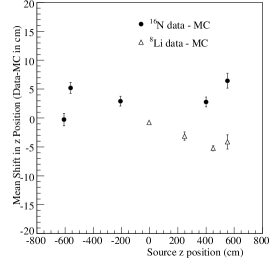
Figure 20: Comparison of vertex accuracy in for $\rm{}^{16}{N}$ and $\rm{}^{8}{Li}$ data for the October 2000 $\rm{}^{16}{N}$ $z$ scan and the December 2000 $\rm{}^{8}{Li}$ scan. Vertex accuracy is defined here as the difference between expected source position (based on the measurements by the source-positioning mechanism for data and the true source position for Monte Carlo simulated events) and reconstructed position. The shifts between the Monte Carlo prediction and the data for both sources are consistent with a model that scales each event’s reconstructed radial position by $\pm$1%.

The $\rm{}^{8}{Li}$ -$\rm{}^{16}{N}$ comparison also serves as a check of the time dependence of the vertex accuracy, since these data were taken at times separated by a few months. We additionally looked at data separated by over a year, using other scans, and this, too, was consistent with the simple $\pm$1% radial scaling model.

VI.1.2 Vertex Resolution

We measured the uncertainty on the vertex resolution in the same way as the vertex accuracy, through comparisons of $\rm{}^{16}{N}$ and $\rm{}^{8}{Li}$ data to Monte Carlo simulation. The resolution is obtained using the Gaussian convolution described in Section VI.1.1 for the different source distributions (Compton scatters for the $\rm{}^{16}{N}$, a spherical shell for the $\rm{}^{8}{Li}$). Figure 21 compares the resolution obtained this way for the October 2000 $z$ scan to the Monte Carlo simulation. Here we see differences in resolution between the data and the Monte Carlo simulation of 1-5 cm, with the data having a systematically broader resolution than the simulation. Such a systematic broadening is not unexpected, as there are many effects in real data which will worsen the resolution relative to the Monte Carlo simulation (shifts in timing calibrations, knowledge of the source position during calibration, knowledge of the true angular distribution of PMT hits around the event direction, etc.) but few if any that will make it better. We nevertheless treat the systematic difference between data and the Monte Carlo simulation as a double-sided uncertainty.

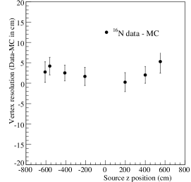
Figure 21: Difference between vertex resolution for October 2000 high rate $z$ scan as a function of $z$ and Monte Carlo prediction.

We also explored the energy ($N_{\rm hit}$) dependence of the resolution, since we expect the resolution to depend on energy ($N_{\rm hit}$) both through the increase in the number of hits available at higher energies as well as the sharper angular distribution of the Cherenkov cone. Figure 22 compares the Monte Carlo prediction of the $N_{\rm hit}$ dependence of the vertex resolution for $\rm{}^{16}{N}$ events to source data and Figure 23 does the same for $\rm{}^{8}{Li}$ data. Both show reasonably good agreement on the magnitude of the resolution (to a few cm) as well as its slope with energy. While the $\rm{}^{8}{Li}$ source data is somewhat suspect because of the blockage of backward light by the source chamber, it is the only data available for testing the Monte Carlo predictions at high energies. While we may be willing to accept the Monte Carlo simulation’s handling of higher energy physics (the scaling of Cherenkov photon production, for example) the effects of more photons (such as crosstalk or a timing bias for multi-photoelectron hits) are not necessarily well-modeled. Figure 23 demonstrates that those uncertainties are not large enough to matter. The fact that the $\rm{}^{8}{Li}$ and the $\rm{}^{16}{N}$ data agree well where they overlap in $N_{\rm hit}$ also suggests that source effects are not significant.

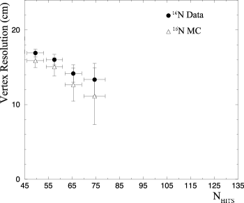
Figure 22: Vertex resolution for high rate $\rm{}^{16}{N}$ data as a function of $N_{\rm hit}$ compared to Monte Carlo prediction.

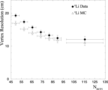
Figure 23: Vertex resolution for $\rm{}^{8}{Li}$ data as a function of $N_{\rm hit}$ compared to Monte Carlo prediction.

Rate-dependent effects were checked using low-rate source data, and we tested time-dependence using source runs taken along different detector axes at times separated by more than a year. In none of these comparisons did we see any effects beyond those shown in the previous figures.

We therefore take as our overall systematic uncertainty on the resolution the rms of the differences between the data and the Monte Carlo simulation shown in Figure 21, which is about 2.5 cm. As mentioned above, we do not shift the resolution in the Monte Carlo simulation to agree with the data, but treat this uncertainty as a double-sided uncertainty (that is, $\pm 2.5$ cm). We estimate the effects of this resolution uncertainty on the neutrino fluxes by convolving the Monte Carlo predicted position pdfs with a Gaussian designed to broaden the Monte Carlo simulation’s resolution function by 2.5 cm. The Monte Carlo prediction for the width of our resolution is 15 cm for $\rm{}^{16}{N}$ events, and we therefore convolved the position pdfs with a Gaussian whose width was 9 cm.

VI.1.3 Summary of Vertex Uncertainties

For the uncertainty in vertex accuracy, we have found that a $\pm$1% radial scaling of the fit position is a reasonable worst-case model for the differences between Monte Carlo simulation and $\rm{}^{16}{N}$ source data. We have further explored the dependence on position, source type, energy, and time and found that in none of these cases is the uncertainty worse than this. For vertex resolution, we have done a similar study, and find that the uncertainty in the resolution is roughly 2.5 cm which is equivalent to convolving a Gaussian of width 9 cm with the Monte Carlo predicted resolution response.

VI.1.4 Angular Resolution

An ideal calibration source for measuring angular resolution would be a directed source of single electrons with tunable energies. The angular resolution function (for a given electron position, direction, and energy) in the detector would then be the distribution of $\theta$, the angle between the reconstructed and the known initial electron directions. While the $\rm{}^{8}{Li}$ source does provide a source of tagged electrons, we do not know the initial directions of individual electrons. Instead, we developed a method for determining the angular resolution and uncertainties using $\gamma$-rays from the ¹⁶N source the:mgb ; the:msn ; the:cj .

The $\rm{}^{16}{N}$ calibration source data can be used to determine angular resolution uncertainty, by relying on the colinearity of Compton scattered electrons with the $\gamma$ direction, when the $\gamma$ loses the majority of its energy. If the scattering vertex, $\vec{r}_{e}$, is known, the $\gamma$-ray direction, $\hat{d}_{\gamma}$, is related to the $\rm{}^{16}{N}$ source position, $\vec{r}_{s}$, by the simple vector relation (See Figure 24)

Figure 24: Diagram showing vectors involved in measurement of angular resolution using the $\rm{}^{16}{N}$ $\gamma$-ray calibration source.

$$\hat{d}_{\gamma}=\frac{\vec{r}_{e}-\vec{r}_{s}}{\mid\vec{r}_{e}-\vec{r}_{s}\mid}$$ (22)

The dot product of this unit vector with the reconstructed event direction gives the cosine of the angle $\theta_{\gamma e}$:

$$\cos\theta_{\gamma e}=\hat{d}_{\gamma}\cdot\hat{d}_{fit}$$ (23)

With the fit vertex $\vec{r_{\rm fit}}$ used as an estimate of the Compton scattering vertex (${\vec{r}_{e}}$) Equation 23 becomes

$$\cos\theta=\frac{\vec{r}_{fit}-\vec{r}_{s}}{\mid\vec{r}_{fit}-\vec{r}_{s}\mid}\cdot\hat{d}_{fit}$$ (24)

Note that this manner of determining the angular resolution depends on vertex reconstruction uncertainties, since the vertex is used to calculate the direction of the Compton scattered electron relative to the incident $\gamma$-ray. In order to minimize the effect of vertex reconstruction errors on the angular resolution measurement, we only used events reconstructing a large distance from the $\rm{}^{16}{N}$ source as compared to the vertex resolution.

Figure 25 shows a comparison of the $\cos{\theta}$ distributions between real and simulated $\rm{}^{16}{N}$ calibration data with the source at the center of the detector. The data plotted are restricted to events that were reconstructed more than 1.5 m from the source position. We see that

Figure 25: The angular resolution tail from $\rm{}^{16}{N}$ is in good agreement with Monte Carlo simulation.

the Monte Carlo model predictions are in good agreement with the measurements for this particular location.

To characterize the angular resolution we define a measure which is the angle between the initial electron direction and the fit direction that contains 68% of the angular distribution. Notice from Figure 26 that this

Figure 26: Angular resolution for Monte Carlo simulated CC electrons. Shown is the distribution of angle between the Monte Carlo predicted initial electron direction and fit direction for $N_{\rm hit}>$65 and $R_{\rm fit}<550$ cm. Roughly 68% of the distribution is contained within 26.7 degrees.

is determined from Monte Carlo simulation to be 26.7^∘ for charged current electrons at energies near that of the ¹⁶N source and within the 550 cm fiducial volume.

The systematic uncertainty on angular resolution is somewhat harder to define than that for the uncertainty on position resolution. The angular resolution is a complicated function as Fig. 26 indicates. As will be discussed later in more detail in Section VIII.5, for our secondary analysis which uses analytic response functions to build pdfs, we fit a parameterized function (Eq. 46) to distributions like that in Figs. 25 and 26. We then created new pdfs with the parameters on the angular response function varied over their $\pm 1\sigma$ uncertainty range, and used the changes measured in the extracted numbers of events as our $\pm 1\sigma$ angular resolution systematic uncertainty. For our primary analysis, in which we used Monte Carlo-generated pdfs, we used a perturbation function to ‘smear’ the pdf. The perturbation function was chosen so that it that reproduced the differences seen in the comparison between data and Monte Carlo simulation like that shown in Fig. 25: a narrowing of the forward peak and the addition of an isotropic component that puts up to 2% of events into the tail. The effects of this smearing are similar to the variations of the analytic angular response function discussed in Section VIII.5.

VI.2 Energy Response

For the integral flux measurements of our initial Phase I results SNO Collaboration (2001, 2002a, 2002a), the dominant uncertainty on our measurements derives from the uncertainty on the detector’s energy scale. The reason is that at the energy threshold used, a small variation in response leads to a large variation in the number of accepted events. The natural covariance between the charged current and neutral current signals—the fact that the differences between the pdfs shown in Fig. 2 are predominantly in the energy distributions—makes the problem significantly worse. We therefore needed to be particularly careful in evaluating these uncertainties.

VI.2.1 Energy Scale

As discussed in Section IV, the energy scale—the number of PMT hits per MeV of electron energy, or the adjustment of reconstructed electron energy to agree with physical electron energy—was determined through deployment of the ¹⁶N source at the detector center. In addition to the center deployment, we also made two extensive scans, covering two orthogonal planes within the detector. The scans were performed in December 1999 and January 2001. The primary estimate of our systematic uncertainty on the energy scale is the volume-weighted average difference between the Monte Carlo model prediction of the detector response to the source at each point and the source data itself. There are many contributors to non-zero differences: the statistics of the calibration source data, small errors in the optical calibrations which are input to the Monte Carlo detector model, and unmodeled or incompletely modeled detector effects such as crosstalk between electronics channels and PMT-to-PMT variations. To account for both the non-zero mean of the volume-weighted difference distribution and its width, we add them linearly and take the sum as our uncertainty on the position-dependence of the energy scale.

Figures  27 and  28 show the fractional differences as a function of the source radial position as well as the volume-weighted distribution of those differences, for one set of position scans. Data taken along the $+z$-axis are excluded from the Figures because the effects of the acrylic vessel neck shift the energy peak substantially. This shift is a small effect on neutrino data because there are so few events which occur in the neck region. The scatter in the points of Fig. 27 that occur for deployments at the same radial position is due to the fact that the source was deployed at different $(x,y,z)$ coordinates for these radii. Based on the December 1999 and January 2001 scans, our $1\sigma$ estimate on the position-dependent energy scale uncertainty for the energy reconstructor is 0.72 %. For the total light ($N_{\rm hit}$) energy estimator, the uncertainty is 1.03%.

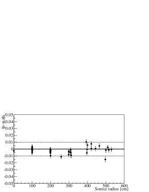
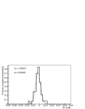
Figure 27: Fractional deviation in effective kinetic energy peak $\mu$ from the Monte Carlo prediction $\mu_{0}$ for December 1999 position scans. Shown in the top frame is the deviation versus source position. The bottom frame shows the distribution of deviations weighted by volume. A conservative $1\sigma$ limit of $0.72\%$ is obtained by adding the mean offset and distribution width linearly. The scatter in the top frame for points at the same radius is due to the fact that these source locations had different $(x,y,z)$ coordinates which gave the same radial positions.

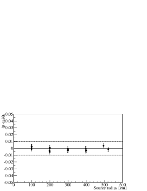
Figure 28: Fractional deviation in effective kinetic energy peak $\mu$ from Monte Carlo prediction $\mu_{0}$ for the January 2001 position scans. Shown in the top frame is the deviation versus source position. The bottom frame shows the distribution of deviations weighted by volume.

We determined the uncertainties associated with source modeling by varying the relevant source description parameters. Details of how this was done can be found in Refs. the:ham ; n16 . The contribution to the uncertainties from source modeling are less than $0.3\%$, and the total source-related uncertainty including uncertainties in the ¹⁶N decay scheme and uncertainty in the tracking of $\gamma$-rays and electrons by EGS4 is $\sim 0.5\%$.

The rate dependence of the calibrated times and charges described in Section V.2 implies that the high rate calibration data ($\sim 200$ Hz) may not correctly characterize the energy scale for neutrino data (typically 20 Hz). Although a rate-dependent correction was applied to the PMT hit times (Section V.2), and the energy calibrator did not use any charge-dependent timing corrections (Section V.5.2), we nevertheless included a small systematic uncertainty to account for residual rate-dependent effects. This uncertainty was determined through comparisons of high and low rate calibration data taken with the ¹⁶N source and the ²⁵²Cf neutron source. These comparisons showed no statistically significant rate-dependent effects, and the resultant uncertainty associated with rate-dependent effects (driven by the statistical sensitivity of the comparisons) was 0.39%.

Variations in channel thresholds can also lead to unexpected changes to the energy scale for neutrino data that are not completely represented by calibration data. The probability of crosstalk between adjacent channels is a very sensitive measure of the channel thresholds, and by monitoring this probability we were able to limit the uncertainty on the energy scale from such variations throughout the neutrino data set to 0.45%. As a verification that the calibration data was not significantly different from the neutrino data, we compared the mean number of noise hits measured with the pulsed trigger (see Section V.5.2) during neutrino data collection to that measured during calibration source runs, and found no significant differences.

In addition to threshold, the gains of the PMTs may also vary and lead to energy scale variations. To measure gain stability, we compared the high edge of the single photoelectron charge peak for neutrino data and ¹⁶N data, and found that the gain was stable to 1.25%. This variation translates into an uncertainty of 0.28% in efficiency, and thus in energy scale.

The complete list of the contributions to the energy scale systematic uncertainties appears in Table 3 where a 0.39% uncertainty is attributed to rate dependence, 0.45% to threshold variations, and 0.28% to gain variations. With the suite of uncertainties added in quadrature, the energy scale uncertainty for the energy calibrator is 1.21%, and for the total light estimator ($N_{\rm hit}$) is 1.39%.

Table 3: Breakdown of systematic uncertainties on energy scale for the total light ($N_{\rm hit}$) energy estimator, and the energy reconstructor.

Contributing factor	$N_{\rm hit}$	$T_{\rm eff}$
		(MeV)
Scale including Time Drift	0.46%	0.25%
Position dependence	1.03%	0.72%
Source	0.46%	0.46%
Rate dependence	0.39%	0.39%
Gain variation	0.28%	0.28%
Threshold variations - XTalk	0.45%	0.45%
Channel accounting	0.1%	negligible
Background noise	0.1%	negligible
Time calibration	negligible	0.5%
Total	1.39%	1.21%

As a cross-check, energy calibration computations have been applied to n(d,t)$\gamma$-ray event data from the ²⁵²Cf source (high and low rate), low rate ¹⁶N data, and pT data.

Figure  29 shows the deviations in the $E_{\rm eff}$ peak for all sources.

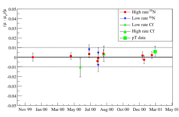
Figure 29: Fractional deviation in kinetic energy peak for all calibration sources including low rate neutron and ¹⁶N data. Here, $\mu$ is the value at the peak for the data, and $\mu_{0}$ is the Monte Carlo simulation’s prediction for the peak.

VI.2.2 Differential Energy Scale Uncertainty

For integral flux measurements, the most important uncertainty on the energy scale is near threshold, where small shifts in the scale can lead to large shifts in the fluxes. Most of SNO’s calibration source data for Phase I (primarily ¹⁶N) have a central value of energy near this threshold. Differential non-linearities in the energy scale can affect the integral measurements, however, because they alter the shapes of the pdfs used for signal extraction. For a spectral measurement, in which each recoil electron energy bin is treated independently, such non-linearities matter more.

The primary sources of potential non-linearity are small errors in the modeling of the PMT hit efficiencies as a function of the number of incident photons (the ‘multiphoton effect’), and detector artifacts that vary with the number of photons such as channel-to-channel crosstalk. For ⁸B solar neutrino events within SNO’s 550 cm fiducial volume the probability of more than one photon hitting a PMT is small, and errors on the modeling of these efficiencies are negligible.

The probability of crosstalk is also small, but it can still lead to one or two additional hits in an event which if ignored could produce a noticeably non-linear scale. The prompt time cut of the energy calibrator removes roughly 2/3 of the crosstalk hits, because their times are delayed slightly. Using 19.8 MeV $\gamma$ rays from the pT source to measure of the shift in energy scale with energy, and interpolating between the ¹⁶N and pT results to the ⁸B spectrum, we limit the additional shift in energy scale from non-linearities to 0.23% at the pT source energy ($T_{\rm eff}=19.1$ MeV), decreasing linearly to zero at the ¹⁶N energy ($T_{\rm eff}=4.98$ MeV).

The functional form for the non-linear piece of the shift in kinetic energy $\delta T_{\rm eff}$ as a function of reconstructed effective energy is

$$\delta T_{\rm eff}=\alpha\times 19.1\times\frac{T_{\rm eff}-4.98}{13.61}$$ (25)

where $\alpha$ is limited to be $\pm 0.0023$. The shift is measured in MeV.

VI.2.3 Energy Resolution

Uncertainties on the detector’s energy resolution have a smaller effect on the measured neutrino fluxes than energy scale uncertainties. Small differences between the true pdfs and the models of those pdfs used for signal extraction do not have a big effect on the overall acceptance. Resolution uncertainties have a much bigger effect on measurements of the backgrounds from low energy radioactivity, as described in Section VII.4.

To measure the uncertainty on energy resolution, we compared the reconstructed energy distributions for calibration data to Monte Carlo simulations of that data, for the 6.13 MeV $\gamma$-ray ¹⁶N source and the 19.8 MeV $\gamma$-ray pT source. For the ¹⁶N source, the measurements were made at many locations throughout the detector volume along the two planes allowed by the calibration system, and for the pT source at several locations along the $z$-axis including positions out to $R\sim 450$ cm.

Figure 16 compares the distribution of reconstructed energy for both data and Monte Carlo simulations of an ¹⁶N deployment near the detector center. To measure the resolution, we fit a Gaussian between 4 and 7 MeV to distributions like those in Fig. 16. We found that on average, the resolution for the data was $\sim$ 2.5% broader than for the Monte Carlo, and that the variations from point to point between the two was also of order 2%. We conservatively added these two measurements linearly, for a combined resolution uncertainty of 4.5%. For the analytic parameterization of the resolution function given in Section VIII.5, there are additional uncertainties associated with the extraction of the parameters from the Monte Carlo simulation. Those uncertainties are given in that section.

For the pT source, we found a much bigger difference between the data and Monte Carlo simulation’s resolutions—roughly 10%, primarily due to the fact that the many neutrons produced by the source affect our ability to measure the resolution in the data, but are not modeled in the Monte Carlo simulation. A linear function was used to interpolate the uncertainties between the ¹⁶N and pT energies:

$$\frac{\Delta\sigma_{T}}{\sigma_{T}}=0.045+0.00401\times(T_{\rm eff}-4.98)$$ (26)

VII Background Measurement

After processing, the events remaining above the analysis threshold and within the 550 cm fiducial volume are primarily recoil electrons and $\gamma$-rays produced in association with neutrino interactions, but may also include instrumental, radioactive, and cosmogenic backgrounds. In this section we describe measurements to determine the residual contamination from each background source.

VII.1 Instrumental Contamination

Although the suite of low-level cuts described in Section V.3 is highly effective at removing instrumental backgrounds, and the subsequent reconstruction and ‘high-level’ cuts reduce residual contamination still further, we must estimate how many events from instrumental sources remain in the final data set.

Instrumental backgrounds are a particularly difficult problem, because it is not possible to model every possible ill-understood non-Cherenkov background source. Instead, we need a method that can determine the background level irrespective of its source.

The method we adopted for this analysis combined the low-level cuts and the high-level cuts in what is sometimes referred to as a ‘bifurcated analysis’ E787 . For more detail than we give here, see Ref. the:vrusu .

In a bifurcated analysis one picks two cuts (or two sets of cuts as we have done) and counts the numbers of events in the data set rejected by either cut, both cuts, or neither cut. We assume that the data set consists of just two classes of events, signal events $\nu$ and background events $\beta$, so that the total number of events in the data set is just $S=\beta+\nu$. The background contamination in the final signal sample is just the fraction of $\beta$ that passes both sets of cuts. If the acceptance for background events by cut set $i$ is $y_{i}$, the final background contamination is $K=y_{1}y_{2}\beta$. If the acceptance for signal events by cut set $i$ is $x_{i}$, the final number of signal events is $x_{1}x_{2}\nu$.

We start with three separate event totals: the number of events that pass both cuts ($a$), the number that fail cut 1 but pass cut 2 ($b$), and the number that pass cut 1 but fail cut 2 ($c$). We then relate all of these with a linear system of equations:

$$a+c=x_{1}\nu+y_{1}\beta$$ (27)

$$a+b=x_{2}\nu+y_{2}\beta$$ (28)

$$a=x_{1}x_{2}\nu+y_{1}y_{2}\beta$$ (29)

$$\beta+\nu=S$$ (30)

which we solve analytically to determine the remaining background contamination $K=y_{1}y_{2}\beta$. The values for the cut acceptances will be discussed later, in Section IX.3.

We illustrate the general approach in Fig. 17, which shows ¹⁶N events events in blue, neutrino candidate events in grey, and instrumental background events in black on a ‘high-level’ cut plot. The in-time ratio (ITR) is on the horizontal axis and the average PMT pair angle $\theta_{ij}$ on the vertical axis. The ¹⁶N data define a ‘Cherenkov box’ (see Section V.6) that contains most of the neutrino event candidates. Most instrumental background events, defined as events which fail the ‘low level’ cuts, lie outside the Cherenkov box. Our bifurcated analysis measures the ratio of the number of events failing the low-level cuts that lie within the Cherenkov box to those that lie outside, and also measures the number of events that pass the low-level cuts but lie outside the Cherenkov box. The number of background events within the Cherenkov box (that is, which pass both the low-level and high-level cuts) is then the product of these two numbers. For the final Phase I data set, we find using this technique that the overall contamination has a $95\%$ confidence level upper limit of $K\leq 3$ events.

The dominant systematic uncertainties in this analysis are the uncertainties on the cut acceptances (see Sections IX.3.1 and IX.3.3) and the possibility of variations in the efficiency of the cuts for removing backgrounds. For the latter, we looked at the stability of each cut as a function of time using calibration source data.

For this analysis to work, the two sets of cuts we use must be orthogonal to one another—we must be sure that the probability of passing the low-level cuts does not increase the probability of passing the high-level cuts. To demonstrate orthogonality, we loosened the cuts (essentially opening the final ‘signal box’ defined by those events which pass both sets of cuts) and measured the increase in the number of background events. With the looser cuts, we found the increase in the number of background events agreed well with what would be expected for orthogonal cuts.

To ensure that there were no instrumental backgrounds missed by this analysis, we also examined many different distributions of events and hits in ‘detector coordinates’—the number of hits as a function of electronics channel (rather than PMT), the distribution of event directions relative to the detector’s zenith (rather than the solar direction), and the general PMT-by-PMT occupancy. We found no evidence of any remaining non-Cherenkov-light background.

In addition, we repeated the bifurcated analysis using different sets of cuts—for example replacing the cut on the mean PMT pair angle with a cut on an event ‘isotropy’ parameter derived from the full two-point PMT-PMT correlation function, or using only a subset of the low-level cut suite. All differences in the results were very small and within our expectations.

VII.2 Photodisintegration Background

By far the most dangerous background to the NC measurement are the neutrons produced through photodisintegration of deuterons by low energy radioactivity. In particular, ²³²Th and ²³⁸U have $\gamma$-rays at the end of their decay chains (2.61 MeV and 2.44 MeV, respectively) that are above the 2.22 MeV deuteron binding energy. Low levels of these nuclei can be found in all the components of the detector: the heavy water, the acrylic vessel, the light water, PMT support structure, as well as the PMT glass and base hardware. The neutrons produced by photodisintegration are indistinguishable from those produced by the NC reaction, and therefore measurements of the background levels inside the detector are crucial for correct normalization of the total ⁸B flux. It is critical to measure the levels of ²³²Th and ²³⁸U separately as the fraction of decays that lead to $\gamma$-rays above 2.2 MeV are very different, 36% and 2%, respectively. Additionally, the photodisintegration cross-section depends strongly on the decay $\gamma$-ray energy.

The first step in dealing with these backgrounds was to build the detector with very stringent radio-purity targets for all components. Table 4 lists the ²³²Th and ²³⁸U target levels for the D₂O, AV, and H₂O. (At these radiopurity levels, the background to the NC signal is approximately 1 neutron produced per day or $\sim$10% of the NC signal). In this section, we describe the techniques developed to measure the ²³²Th and ²³⁸U concentrations in different detector regions, and the resultant numbers of background neutrons which these measurements imply.

Table 4: The target radio-purity levels for different components in the SNO detector.

Component	232Th	238U
	(g/g)	(g/g)
D2O	3.7$\times$10-15	4.5$\times$10-14
H2O	3.7$\times$10-14	4.5$\times$10-13
AV	1.9$\times$10-12	3.6$\times$10-12

As in the rest of the analysis, we used two independent approaches to measuring backgrounds within the H₂O and D₂O. Methods that remove water from the detector and perform direct radioassays to determine the concentration of impurities are called ex-situ techniques, and methods that measure background levels using the Cherenkov light observed within the SNO detector are called in situ.

VII.2.1 Ex-situ Techniques for Determining Water Radioactivity

The ex-situ techniques circulate large samples of water from the detector volumes, extract background isotopes from the samples, and count the number of decays using instrumentation external to the SNO detector. We developed three such ex-situ techniques: extraction of Ra isotopes using manganese oxide (MnO${}_{\mbox{x}}$) beads T. C. Andersen et al. (2003a), extraction of Ra, Th and Pb isotopes using hydrous titanium oxide (HTiO)-loaded membranes T. C. Andersen et al. (2003b), and degassing the ²²²Rn from the ²³⁸U chain (the “Rn assay”, Ref. I. Blevis et al. ).

In the MnO${}_{\mbox{x}}$ technique, D₂O or H₂O is passed through polypropylene columns that contain beads coated with a manganese oxide compound, which extracts Ra from the flowing water. After a large volume of water has passed through the columns, they are removed and dried. The dried columns are then attached to a gas flow loop on an electrostatic counter. The Rn produced from Ra decay is swept from the columns into the electrostatic counter where it decays. The charged Po ions from the decay of Rn are carried by the electric field onto an $\alpha$ counter where the decays of the Po are detected, and their $\alpha$ energy spectra are collected. For the ²³²Th chain, the relevant Po $\alpha$ decays are ²¹⁶Po (6.8 MeV $\alpha$) and ²¹²Po (8.8 MeV $\alpha$), whereas the relevant ones for the U chain are ²¹⁸Po (6.0 MeV $\alpha$) and ²¹⁴Po (7.7 MeV $\alpha$). A number of MnO${}_{\mbox{x}}$ assays were carried out for both the D₂O and H₂O. The ²³²Th value for the MnOx data, averaged over the neutrino livetime, for Phase I of the experiment is

$$\mbox{D${}_{2}$O}: 2.15\,^{+0.90}_{-0.94}\,\times\,10^{-15}\ \mbox{g Th/g D}_{2}\mbox{O}$$

$$\mbox{H${}_{2}$O}: 8.1\,^{+2.7}_{-2.3}\,\times\,10^{-14}\ \mbox{g Th/g H}_{2}\mbox{O}$$

where the statistical and systematic uncertainties have been combined in quadrature. Ref. T. C. Andersen et al. (2003a) provides a more detailed discussion of the evaluation of the systematic uncertainties.

In the HTiO technique T. C. Andersen et al. (2003b), D₂O or H₂O is passed through hydrous titanium oxide (HTiO) trapped on filtration fibers. The HTiO ion-exchanger is first deposited onto a microfiltration membrane. Then columns containing the loaded filters are used to extract ²²⁴Ra (from the Th chain) and ²²⁶Ra (from the U chain) from a large volume of D₂O or H₂O. After extraction, the Ra is eluted with nitric acid, and subsequently concentrated to $\sim$10 m$l$ of eluate. This is then mixed with liquid scintillator and counted using $\beta$-$\alpha$ delayed coincidence counters the:taplin . For the ²³²Th chain, the coincidences of the $\beta$-decay of ²¹²Bi and the $\alpha$-decay of ²¹²Po are counted, whereas the coincidences of the $\beta$-decay of ²¹⁴Bi and the $\alpha$-decay of ²¹⁴Po are counted for the ²³⁸U chain. The HTiO and MnOx measurements were in good agreement, but the MnOx result above was used as the final ex-situ measurement of the ²³²Th concentration because the measurements were made more regularly.

The measurements of ²²⁶Ra concentration in the D₂O and the H₂O by the MnO${}_{\mbox{x}}$ and the HTiO techniques described above are not, however, sufficient to determine the total radioactive background from the ²³⁸U chain. Even a small ingress of underground laboratory air (with its $\sim$3 pCi/$l$ of ²²²Rn) can lead to significant disequilibrium between ²²⁶Ra and ²¹⁴Bi. To tackle this problem, we developed a Rn assay technique I. Blevis et al. . Water drawn from discrete sample points in the detector is flowed through a degasser to liberate Rn. The Rn is purified and collected in a cryogenic collector. The subsequent $\alpha$ decays are counted in a Lucas cell scintillator (ZnS) chamber on a 2.54-cm diameter photomultiplier tube. Since there is a delay of many ²²⁰Rn lifetimes between the preparation of the Lucas cells and their subsequent counting, this method is sensitive only to ²²²Rn decays.

The Rn assay results for different sampling points in the D₂O and the H₂O as a function of time and systematic uncertainties in the results are discussed further in Ref. I. Blevis et al. . It can be seen from the measurements presented there and here in Fig. 30 that during the early phase of the production running, the Rn level in the detector was much higher than our target level. After a few months the levels dropped, and remained better than the target levels, with the exception of some excursions for short intervals.

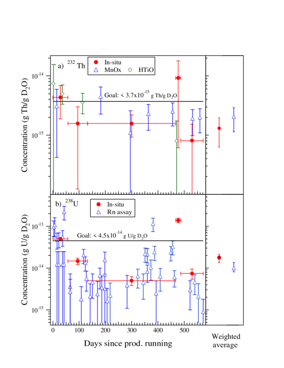
Figure 30: Comparing the ex-situ and in-situ results as a function of time.

VII.2.2 In-situ Technique for Determining Water Radioactivity

The in-situ technique identifies and measures the different radioactive backgrounds using the Cherenkov light produced by the events within the SNO detector itself. The goal of the in-situ analysis is twofold: first to separate decays from the ²³⁸U chain from those of the ²³²Th chain, and second to determine the corresponding radioactivity levels based on the total numbers counted. We applied this analysis to both the D₂O and H₂O. Unlike the ex-situ analysis, the in-situ analysis is integrated over the same livetime as the neutrino data, rather than being sampled at discrete times. Moreover, it measures the amounts of the radionucludies, ²⁰⁸Tl and ²¹⁴Bi (from the ²³²Th and ²³⁸U decays chains, respectively), that give rise to $\gamma$ rays above 2.2 MeV. The in-situ technique measures the isotopes that produce photo-disintegration backgrounds directly and does not assume secular equilibrium in the decay chain. As in the ex-situ analysis described above, we are interested in this analysis in measuring the overall detector radioactivity, and from that measurement calculating the number of neutrons produced in the decays of the associated daughters. We therefore used a lower energy threshold than our nominal signal analysis threshold of $T_{\rm eff}=5.0$ MeV, to ensure that we had enough background statistics to make a meaningful measurement. Although the $Q$ values of many of the radioactive decays we are studying are below even this lower threshold, the broad energy resolution of the detector leads to a substantial number that reconstruct above threshold. For more detail, see Refs. the:chen ; the:mcgregor .

The ²⁰⁸Tl decay has a $Q$ value of $\sim$5.0 MeV, and the ²¹⁴Bi decay a $Q$ value of 3.27 MeV. Almost every ²⁰⁸Tl decay emits a 2.614 MeV $\gamma$, one or more low energy $\gamma$s and a $\beta$ with an endpoint of $\sim$1–1.8 MeV, whereas there is a unique branch in the ²¹⁴Bi decay to the ground state of ²¹⁴Pb that produces a single $\beta$ with an endpoint energy of 3.27 MeV. Above an analysis threshold of $T_{\rm eff}\sim 3.8$ MeV, the detected events from ²¹⁴Bi decays are dominated by the 3.27 MeV endpoint $\beta$-decay electrons, while those from ²⁰⁸Tl decays may have multiple energetic electrons produced by Compton scattering as well as $\beta$-decay. The ²¹⁴Bi decays will therefore have a PMT hit pattern resembling that of a single electron, while ²⁰⁸Tl decays appear more isotropic.

The different hit patterns of ²¹⁴Bi and ²⁰⁸Tl events allowed us to use the distribution of event ‘isotropy’ (characterized by the mean angle between PMT pairs, $\theta_{ij}$) to separate the ²⁰⁸Tl  and ²¹⁴Bi decays statistically. (The energy spectra from these decays are too similar above 3.8 MeV to allow separation using pdfs in event energy). The parameter $\theta_{ij}$ is calculated by taking the average angle relative to the reconstructed event vertex for all hit PMT pairs within a prompt light time window in an event. It is the same variable as was used as one of our ‘Cherenkov box’ cuts, as discussed in Sections V.3 and VII.1.

Figure 31 shows the Monte Carlo model’s prediction of the difference in the distribution of $\theta_{ij}$ between ²⁰⁸Tl and ²¹⁴Bi decays. Statistical separation of the ²⁰⁸Tl and ²¹⁴Bi events is obtained by a maximum likelihood fit to the $\theta_{ij}$ distribution of the Cherenkov events.

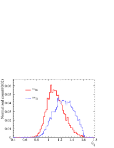
Figure 31: Monte Carlo-predicted event isotropy distributions for ²⁰⁸Tl and ²¹⁴Bi decays. The isotropy parameter shown here on the abscissa, $\theta_{ij}$, is the average opening angle between all fired photomultiplier tube pairs centered at the reconstructed event vertex. More isotropic light distribution in an event results in a higher $\theta_{ij}$ value.

The in-situ analysis of background radioactivity in the D₂O has its own background—events from the H₂O region which misreconstruct into the D₂O volume and therefore look like D₂O radioactivity. To avoid this ‘background to the background’, the in-situ analysis was done using a smaller fiducial volume ($R_{\rm fit}<450$ cm) than the 550 cm fiducial volume used for the neutrino analysis. Ultimately, the concentrations of radioactivity determined from the in-situ analysis are scaled to the full volume. The second background in the in-situ analysis is the neutrino events themselves, and to avoid these a narrow ‘monitoring’ window in energy is chosen, $N_{\rm eff}=33-36$, which corresponds to the energy range $T_{\rm eff}\approx 3.8$ MeV to $T_{\rm eff}\approx 4.2$ MeV (see Section V.5.2 for a discussion of the relationship between $N_{eff}$ and energy).

In the in-situ analysis of the H₂O background, a slightly different energy window was used, from $T_{\rm eff}\sim$4.0 MeV to $T_{\rm eff}\sim 4.5$ MeV. The higher energy window was used because of increased contamination from other background sources (e.g., $\beta-\gamma$ decays from the PMT array). The fiducial volume for the H₂O analysis was chosen to be far from the acrylic vessel and D₂O volume but well within the angular acceptance of the PMTs and light concentrators, 650 cm$<R<$680 cm. Selection of events with an outward-going reconstructed direction further reduced contamination.

From the in-situ analysis the equivalent ²³²Th and ²³⁸U concentrations in the D₂O are:

232Th:	1.34 $\pm$ 0.62 ${}^{+0.33}_{-0.38}$ $\times$ 10-15 g Th/g D2O
238U:	17.8 $\pm$ 1.4 ${}^{+3.2}_{-4.1}$ $\times$ 10-15 g U/g D2O.

where the first uncertainty is statistical and the second systematic.

The dominant systematic uncertainties in the in-situ study of D₂O radioactivity are in the energy scale and in the $\theta_{ij}$ pdfs. As is true for the neutrino pdfs, these $\theta_{ij}$ pdfs were derived from the Monte Carlo simulation. We verified their shapes by comparing them to the distributions obtained during periods of Rn ingress into the target volume.

Temporal variation of the detector energy scale was modeled to study its effect on the extracted ²³²Th and ²³⁸U concentrations. We have included in the systematic uncertainties those due to contamination from other background sources in the monitoring window. In addition, we have included uncertainties due to potential non-uniformities of the spatial distributions, and thus the numbers represent the estimate of the total radioactivity in the D₂O, not just that within $R<450$ cm.

Similarly, the equivalent ²³²Th and ²³⁸U concentrations in the H₂O  determined from the in-situ analysis are:

232Th:	14.2 $\pm$ 0.6 $\pm$ 6.6 $\times$ 10-14 g Th/g H2O
238U:	75.5 $\pm$ 1.2 $\pm$ 32.9 $\times$ 10-14 g U/g H2O.

where again the statistical uncertainty is listed first.

The systematic uncertainties in the H₂O analysis are considerably larger than those in the D₂O analysis, with the largest component in the H₂O analysis being the contribution from the energy scale uncertainty, whose magnitude is 42% of the measured ²³²Th and ²³⁸U concentrations. The large uncertainty is due, in part, to the fact that the optics of the outer regions of the detector are difficult to model (particularly the optics of the PMT and concentrator assembly), and that we calibrated these outer regions less frequently than the inner fiducial region.

VII.2.3 Overall ²³²Th and ²³⁸U Concentration Determined for the Water

The in-situ and ex-situ techniques are independent, and their systematic uncertainties have been independently assessed. Fig. 30 shows good agreement between ex-situ (²³²Th: MnOx, ²³⁸U: Rn assay) and in-situ measurements. For the ²³²Th chain, we have therefore used the weighted mean of the results, including additional uncertainties associated with the ex-situ sampling. The ²³⁸U chain activity is dominated by Rn ingress, which is highly time dependent, and we have therefore used the in-situ determination for this activity as it includes the appropriate weighting of neutrino live time. For the present data set, we find the equivalent equilibrium ²³⁸U and ²³²Th concentrations in the D₂O to be

$${}^{232}\mbox{Th} : 1.61\pm 0.58\times 10^{-15}\mbox{g Th/g D${}_{2}$O}$$

$${}^{238}\mbox{U} : 17.8^{+3.5}_{-4.3}\times 10^{-15}\mbox{ g U/g D${}_{2}$O},$$

where we have added the statistical and systematic uncertainties in quadrature. The concentrations in the H₂O are

$${}^{232}\mbox{Th} : 9.1\pm 2.7\times 10^{-14}\mbox{g Th/g H${}_{2}$O}$$

$${}^{238}\mbox{U} : 75.5\pm 33.0\times 10^{-14}\mbox{ g U/g H${}_{2}$O}.$$

VII.2.4 Acrylic Vessel Radioactivity

To determine the photodisintegration background due to radioactivity in the walls of the acrylic vessel, we first need to establish the vessel’s radioactivity load. It is difficult to apply the in-situ technique, primarily because the vessel is very clean and its Cherenkov signals are masked by the dominant H₂O background. The approach here is therefore to first determine the radioactivity load of the acrylic vessel from radioassay results, and then to use Monte Carlo simulations to deduce the photodisintegration background. We discuss below contributions to the radioactivity from the acrylic vessel panels and bonds, from surface activity caused by mine dust, and from a ‘hot spot’ of unknown origin.

During the production of the AV panels, acrylic samples were analyzed for internal ²³²Th and ²³⁸U radioactivities by neutron activation analysis. The ²³²Th concentration in the thermoformed acrylic panels was found to be 0.25$\pm$0.04 ppt ²³²Th.

Additional radioactivity was presumably introduced during bonding of the acrylic panels, possibly from the glue, environmental dust, or plating of radioactive isotopes. It is difficult to determine this background, as dust might be embedded in the bond during the construction. The surface area and volume of the bonds are much smaller than those of the vessel as a whole, and therefore we estimate an uncertainty of ${}^{+1}_{-0}$ $\mu$g ²³²Th ($\sim$ total amount of Th from dust on the inner surface of the vessel) due to embedded dust in the bonds. Adding this in quadrature to the uncertainty of the Th concentration in the thermoformed panels, we estimate 7.5${}^{+1.7}_{-1.3}$ $\mu$g of ²³²Th for the full vessel. This represents an expected 6.2${}^{+1.4}_{-1.1}$ detected photodisintegration neutrons in the full Phase I data set.

Since the U contribution to the backgrounds is less than ²³²Th for a given concentration and the U-to-Th ratio in materials is normally less than 1, the ²³⁸U concentration in the vessel did not pose as significant a problem as ²³²Th. Neutron activation of virgin acrylic samples gave 2$\sigma$ upper limits ranging from 0.1 ppt to 1 ppt ²³⁸U. We therefore estimate 0.5$\pm$0.5 ppt ²³⁸U as the total contamination, under the assumptions that the thermoforming process introduced the same amount of ²³⁸U into the panels as Th ($\sim$0.2 ppt) and that the embedded dust in the bonds has the same U-to-Th ratio as mine dust. This translates to 15$\pm$15 $\mu$g ²³⁸U in the vessel.

During its construction and after final cleaning, the areal density of ²³²Th deposited on the surface of the acrylic vessel was determined from X-ray fluorescence (XRF) analysis of dust samples lifted off the vessel’s surface by adhesive tapes. The amount of ²³²Th on the acrylic vessel determined from the XRF analysis after its final cleaning was found to be:

Inner AV surface:	0.87 $\pm$ 0.17 $\mu$g 232Th
Outer AV surface:	0.96 $\pm$ 0.19 $\mu$g 232Th.

The ²³⁸U load could not be determined directly from the dust sample because of the limited sensitivity of the XRF. The dust sample was assumed to have the same composition as mine dust—a ²³⁸U/²³²Th ratio of 0.187$\pm$0.024. The amount of ²³⁸U on the acrylic vessel is then:

Inner AV surface:	0.16 $\pm$ 0.04 $\mu$g 238U
Outer AV surface:	0.18 $\pm$ 0.04 $\mu$g 238U.

As discussed in Section V.8 and shown in Fig. 18, an anomalous ‘hot spot’, which appears to be radioactivity embedded in the acrylic vessel, was identified during analysis of Cherenkov events near the edge of the fiducial volume. We derived an estimate of the radioactivity level of the hot spot using data from low energy calibration sources (for example, ²³²Th embedded within acrylic) as well as extensive Monte Carlo simulations that included variations of the optical properties of the vessel. Based on these analyses, we find that under the hypothesis that the radioactivity $m_{hs}$ of the hot spot is all Th (the worst case), its level is:

$$m_{hs}\;=\;10\,\pm\,1\,\mbox{(stat.)}\,^{+8.5}_{-3.5}\,\mbox{(sys.)}\,\mu\,\mbox{g Th equivalent}.$$

We assumed in these analyses that the hot spot was located on the outer surface of the acrylic vessel. The dominant systematic uncertainty was the uncertainty of the energy scale at the acrylic vessel. Because of the complicated light propagation in the acrylic vessel, the systematic uncertainty associated with the energy response was estimated at $\sim$30%. Although we assumed the hot spot was comprised solely of Th-chain radioactivity, our studies indicated that there are compensating effects among Q values, detector efficiencies, neutron propagation, and photo-disintegration rates for $\gamma$s that cause the estimated photodisintegration neutron rate to be relatively constant regardless of the relative ²³⁸U and ²³²Th composition.

VII.3 Determining the Total Photodisintegration Background

Monte Carlo calculations were performed to determine the equivalent ²³²Th and ²³⁸U quantities in different detector regions that would produce one photodisintegration neutron in the D₂O per day. Table 5 summarizes these results.

Table 5: Equivalent ²³²Th and ²³⁸U masses that each produce a photodisintegration neutron in the D₂O target per day. Radioactivities are assumed to be in secular equilibrium and evenly distributed in the respective detector regions. The uncertainties shown here are statistical. Systematic uncertainties are dominated by the uncertainty in the cross section, which is $\sim$1%.

	232Th	238U
	($\mu$g)	($\mu$g)
D2O	3.79$\pm$0.01	29.8$\pm$0.76
AV	10.83$\pm$0.04	82.92$\pm$1.75
H2O	278.3$\pm$5.2	2325$\pm$111

Using the ²³²Th and ²³⁸U concentrations, the equivalent masses in Table 5, and the neutron detection efficiency for $T_{\rm eff}>5$ MeV and a fiducial volume of $R_{\rm fit}<550$ cm, we find the expected total number of detected photodisintegration neutrons arising from internal radioactivities from different detector components to be 71.3${}^{+11.6}_{-11.9}$ counts, which is 12% of the expected neutral-current signal.

Contributions from different regions are summarized in Table 6. Calibrated neutron detection efficiencies (see Section IX.5) were used in these calculations.

Table 6: Summary of the estimated number detected photodisintegration neutrons ($T_{\rm eff}>5$ MeV) in the fiducial volume ($R_{\rm fit}<$550 cm.) for Phase I of the experiment

	232Th	238U	Total
	(counts)	(counts)
D2O	18.4$\pm$6.5	25.9${}^{+5.0}_{-6.3}$	44.3${}^{+8.2}_{-9.1}$
AV	14.2${}^{+5.8}_{-6.6}$	1.6$\pm$1.6	15.8${}^{+6.0}_{-6.8}$
H2O	5.6${}^{+3.6}_{-2.2}$	5.6${}^{+4.2}_{-2.9}$	11.2${}^{+5.5}_{-3.6}$
Total	38.2${}^{+9.4}_{-9.5}$	33.1${}^{+6.7}_{-7.1}$	71.3${}^{+11.6}_{-11.9}$

VII.3.1 Other Possible Sources of Photodisintegration

In the following we briefly discuss other possible sources of photodisintegration.

1. $\beta-\gamma$ from the PMTs and PSUP structure
   For U and Th decays in the PMT/PSUP region to photodisintegrate a deuteron, the $\gamma$s emitted must travel a very long distance ($>$10 attenuation lengths). A Monte Carlo study was performed to estimate the photodisintegration background due to these decays in the PMT/PSUP region. Based upon this study, we estimate an upper limit of 0.009 neutron captures per day in the fiducial volume, corresponding to $<$1.4 neutrons detected for the full Phase I data set.

2. Outer H₂O $\beta-\gamma$
   Radioassay results demonstrate that the H₂O outside the photomultiplier tube support structure has an average ²³⁸U concentration very similar to that in the inner H₂O (i.e. between the acrylic vessel and the PSUP). Because of the large radial attenuation of neutrons produced in the outer region of the detector, we concluded that contributions to the total photodisintegration background from the cavity H₂O are negligible.

3. Sources other than Th/U
   An extensive literature search was made for long-lived isotopes with high energy $\gamma$ decays that could be present in the heavy water. The only possibilities found were those that could have been produced had the water been used in a reactor. As the SNO heavy water was never used this way, there are no isotopes known to us other than ²³²Th and ²³⁸U that are capable of producing photodisintegrating $\gamma$-rays.

VII.4 Low Energy $\beta$-$\gamma$ Backgrounds

The number of events originating within the D₂O volume that appear above threshold is kept small primarily by ensuring that the radioactivity levels in the heavy water are low. In addition to the neutrons produced through photodisintegration, the primary particles from decays of U and Th daughters (low energy $\gamma$s and $\beta$s) can also lead to events in the final data sample. Although nearly all decays in these chains have Q values lower than the $T_{\rm eff}=5.0$ MeV analysis threshold, the broad energy resolution of the detector at low energies allows a small fraction of these decays to appear above threshold. We refer to backgrounds in the D₂O as $\beta$-$\gamma$ backgrounds to distinguish them from the neutron backgrounds described above.

Outside the heavy water volume, however, the acrylic vessel, the light water, and in particular the PMT array and support structure have relatively high levels of radioactivity. The vast majority of these events (as well as of high energy $\gamma$-rays coming from the cavity walls) are removed by the 550 cm fiducial volume cut (see Section V.8).

We therefore have two distinct approaches to these two classes of backgrounds: for events originating within the heavy water the dominant issue is how well we understand the energy response of the detector, while for events originating outside we must know the reconstruction accuracy well.

VII.4.1 Internal to D₂O Volume

As described in Sections IV and VI, the Monte Carlo model is well calibrated within the fiducial volume, reproducing the measured energy spectra of different sources over a range of energies covering nearly the entire solar neutrino energy regime. With the exception of the energy scale itself, the model parameters were derived independently from the calibration sources—thus the successful simulation of the source data is the result of the physical basis of the model itself. We therefore can reasonably expect that the model will accurately simulate the characteristics of other radioactive decays that differ only in the physical particles they produce.

Our approach to estimation of these low energy $\beta$-$\gamma$ backgrounds was to simulate Tl- and Bi- chain decays for each run in the SNO data set, and to apply the analysis chain described in Section V to these simulated data. To minimize uncertainties associated with analysis efficiencies, we do not use the Monte Carlo to make an absolute prediction of the number of events above threshold, but to predict the ratio of the number of detected $\beta$-$\gamma$ events to the number of detected photodisintegration neutrons. This ratio is then normalized by using the predictions for the number of photodisintegration neutrons from the ex-situ radioassay and in-situ Cherenkov analyses described in Sections VII.2.1 and VII.2.2.

Based upon the Monte Carlo simulation, the energy spectra for $\beta$-$\gamma$ events are well represented by simple Gaussians in the energy range $4.5<E<6.5$ MeV. The mean ($\mu$) and width ($\sigma$) from these fits are 2.019 MeV and 0.8773 MeV for ²⁰⁸Tl decays, and 2.588 MeV and 0.7828 MeV for ²¹⁴Bi decays.

To determine the systematic uncertainties on the ratio of the numbers of $\beta$-$\gamma$ events to photodisintegration neutrons, we began with the uncertainties on the Monte Carlo model described in Section VI and on all applied cuts (described later in Sections IX.3.1 and IX.3.3). We then created 10000 ‘hypothetical’ SNO experiments whose energy scale, resolution, vertex accuracy, etc., were slightly different from the baseline Monte Carlo prediction by amounts consistent with the measured uncertainties on each of those quantities. For each hypothetical experiment the ratio of $\beta$-$\gamma$ events to photodisintegration neutrons was calculated for each decay chain, and a 1$\sigma$ confidence interval was determined from the distribution of the ratio over the 10000 trials.

With $T_{\rm eff}>$5.0 MeV and $R_{\rm fit}<$550 cm, the ratios between the numbers of detected $\beta$-$\gamma$ events to detected photodisintegration neutrons are:

208Tl:	0.162 ${}^{+0.092}_{-0.030}$
214Bi:	0.670 ${}^{+0.460}_{-0.125}$.

Given the estimated numbers of detected photodisintegration neutrons (Th: 18.4$\pm$6.5, U: 25.9${}^{+5.0}_{-6.3}$, see Section VII.3), the expected numbers of $\beta$-$\gamma$ events from these decays in the final data set are:

232Th:	3.0 ${}^{+2.0}_{-1.3}$ counts
238U:	17.4 ${}^{+12.4}_{-5.3}$ counts
Total:	20.4 ${}^{+12.6}_{-5.5}$ counts.

As a test of this method, we used data taken during two periods in which the radon levels in the detector were 1-2 orders of magnitude higher than their nominal levels. As can be seen in Fig. 30, the first of these ‘high radon’ periods occurred near the start of data taking, while the initial radon load was decaying away, and the second period occurred roughly 90% through the run, when a pump failed and allowed radon to enter the D₂O volume. Using the method described above, we predicted the excess number of events as a function of energy during these periods and found good agreement with the data.

We also compared the Monte Carlo predictions and uncertainties to data taken with shielded low energy Th sources. The shield was intended to allow only $\gamma$-rays from the source to be seen by the detector, so that uncertainties associated with the optics of $\beta$-originated Cherenkov light within the source itself could be ignored.

Figure 32 shows the final estimate for the number of $\beta$-$\gamma$ decays that make it into the final neutrino data set. The curves shown are not a fit to the data set—they are normalized by the in-situ and ex-situ background estimates and simply overlaid on the data. The widths of the bands indicate the uncertainties on the estimates.

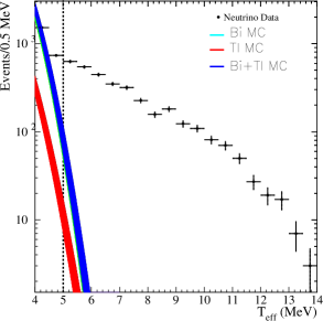
Figure 32: Comparison of Monte Carlo predictions of $\beta$-$\gamma$ background energy spectrum within the D₂O to the total neutrino data set. The curves are not fit to the data, they are normalized by the in-situ and ex-situ estimates and simply overlaid on the neutrino energy spectrum.

VII.4.2 External to D₂O Volume

Radioactive decays within the acrylic vessel itself, the light water region, and the photomultipliers and associated support structure can also produce events above the analysis energy threshold and within the fiducial volume. Events leak into the fiducial volume in two ways: $\gamma$-rays can travel unscattered from their external origin into the fiducial volume, and events occurring outside the volume may be reconstructed incorrectly inside. Although the probability of such leakage is very small, and the probability that such events will be above the analysis energy threshold is also very small, the radioactivity levels outside the heavy water volume are significantly higher than inside, and the leakage can therefore be a non-negligible background to the neutrino signal.

For these backgrounds, neither the Monte Carlo nor analytic models are likely to be good representations of the detector response, for several reasons. First is that the detector is not nearly as well calibrated outside the fiducial volume as inside: the optical and primary energy calibration sources can be deployed in a much more limited number of places outside the heavy water than inside. In addition, there is greater optical complexity in the outer regions of the detector—the PMT angular response at high incidence needs to be understood, the optical shadowing of the photocathodes by the light concentrators becomes important, and the PMT-to-PMT variations in efficiency are amplified as one gets nearer a particular area of the PMT support structure. Lastly, event leakage from this region into the inner volume is caused by highly unusual circumstances, and the leakage fraction may therefore be sensitive to detector artifacts such as electronic crosstalk, miscalibrated PMT timing response, or coincidences between instrumental and radioactive backgrounds.

We therefore based the analysis of these ‘external’ backgrounds primarily on Th and U calibration source data, using the source data to create radial profiles (pdfs in $R^{3}$) of the backgrounds and fitting these profiles to the neutrino data. To determine that the calibration sources’ $R^{3}$ profiles were reasonably insensitive to the specifics of the source type and geometry, we compared the profile obtained using U calibration source data to that obtained using Th calibration source data, and also compared these radial profiles to those obtained with a set of shielded U and Th calibration sources. The shield blocked Cherenkov light created by the $\beta$-decay in the sources’ acrylic encapsulation.

To build the pdfs in $R^{3}$, we used data taken with the acrylic-encapsulated U and Th sources at many discrete locations within the H₂O. To create pdfs appropriate for the uniform distribution of radioactivity expected in the neutrino data, we then weighted the source data by run time, and by volume by taking equal volumes around the source position. Since the sources were untriggered, we subtracted the neutrino (and intrinsic background) signals accumulated during the source run, as well as photodisintegration neutrons (from $\gamma$s entering the heavy water region).

Figure 33 shows the $R^{3}$ pdf derived from U source data compared to a pdf created using neutrino data taken during a period of high radon levels in the light water region. We can see that the two agree well, despite the fact that one is built from calibration data taken at discrete locations and the other from a distributed source of Rn. In Fig. 33 and in other $R^{3}$ distributions, we measure $R^{3}$ in units of cubic AV radii: $R^{3}\equiv(R_{\rm fit}/R_{AV})^{3}$. At the 600 cm AV radius, $R^{3}=1$.

Figure 33: Comparison between the PDF obtained from the high-low radon study and the H₂O pdf derived from acrylic source data. A value of $R^{3}=1$ corresponds to the radius of the AV.

To determine the relative contributions of each of the three sources of background events (acrylic, H₂O, and PSUP), we fit a linear combination of the three $R^{3}$ pdfs to the $R^{3}$ distribution of the data. One problem with this approach is the lack of sufficient statistics in the pdfs at the neutrino analysis threshold of $T_{\rm eff}$=5 MeV—even with very hot calibration sources, it is difficult to get events above the analysis threshold. To overcome this problem, we performed the fit exclusively within the H₂O region, where these backgrounds are highest (the radial range $1.02<R^{3}<2.31$) and with an energy selection of $T_{\rm eff}>$4 MeV. The fit amplitudes for the three background components were then scaled to the intended kinetic energy threshold of 5 MeV. The basic assumptions in this analysis are that there is no correlation between $R^{3}$ and energy, and that the reconstruction does not get worse with higher energy. Several studies were performed to determine how various effects (e.g. pile-up, crosstalk, or high noise rates) can affect reconstruction. None of the studied effects cause a significant effect in the reconstruction—the probability of misreconstruction generally increases rather than decreases as energy is lowered.

Figure 34 shows the results of this $R^{3}$ fit. The band shown in this plot is the range of the systematic uncertainties. For such a plot, we do not necessarily expect the data points to be centered within the band, because the systematic uncertainties are not normally distributed. Some of the sources of systematic uncertainty in this analysis are similar to those for the neutrino analysis described in Section VI, such as vertex accuracy and energy scale. In addition, we evaluated uncertainties associated with the difference between the different radioactive sources (U vs. Th) and the sensitivity of the fit to the radial window chosen. The overall uncertainties for the three sources of external $\beta$-$\gamma$ events are ${}^{+31.7\%}_{-91.3\%}$ for events whose source was the acrylic vessel, ${}^{+29.6\%}_{-9.1\%}$ for events whose source was the light water region, and ${}^{+44.2\%}_{-11.1\%}$ for events from the PMT array.

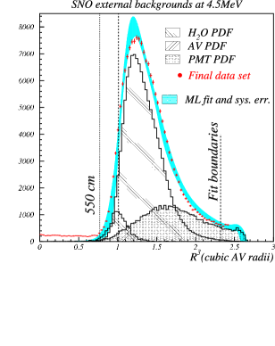
Figure 34: Fit of of $R^{3}$ pdfs created using calibration source data to the neutrino data set, using an energy threshold of $T_{\rm eff}>4.0$ MeV. The extended maximum likelihood method was used in the fit, and the band represents the systematic uncertainties. The $y$-axis is in units of Events/0.03 cubic AV radius.

Although the pdfs which were used in the fits above were binned, analytic forms are used later in the data analysis for the extraction of the CC, ES, and NC neutrino signals (see Section VIII). The analytic form of the $R^{3}$ profile for the PMT $\beta$-$\gamma$ backgrounds is an exponential (with $R^{3}$ in units of cubic AV radii):

$$f(R^{3})\;=\;\exp(-4.538+7.131R^{3})\,+\,1.631.$$

while the energy spectrum ($T_{\rm eff}>$4 MeV) of the PMT $\beta$-$\gamma$ background can be approximated by a Gaussian distribution with $\mu$=1.416 MeV and $\sigma$=0.960 MeV. For the AV $\beta-\gamma$s, the $R^{3}$ distribution can be approximated by a Gaussian with $\mu$=1.056 and $\sigma$=0.1267. The energy spectrum ($T_{\rm eff}>$4 MeV) of the AV $\beta-\gamma$ background can be approximated by a truncated Gaussian distribution with $\mu$=3.441 MeV and $\sigma$=0.4617 MeV.

A number of consistency checks were done to ensure the validity of the results. A separate estimate of the external $\beta$-$\gamma$ tail background was made by calculating the ratio of the count rate within a monitoring window around the acrylic-encapsulated calibration source ($\Omega_{1}$) to that in a window within the fiducial volume ($\Omega_{2}$, $R_{\rm fit}<$550 cm). By counting the number of events in $\Omega_{1}$ during the neutrino runs, the $\beta$-$\gamma$ tail contribution in $\Omega_{2}$ can then be estimated by scaling. The scaled rate was found to be consistent with the results obtained from the $R^{3}$ fit. In addition, one can use the Monte Carlo to predict, based on the radioactivity level of each detector region, the number of tail events above the analysis threshold. These Monte Carlo results were also found to be in agreement with the results described above.

Table 7 is a summary of all estimated $\beta$-$\gamma$ backgrounds with $T_{\rm eff}>$5 MeV which reconstruct within the fiducial volume ($R_{\rm fit}<$550 cm.).

Table 7: Summary of $\beta$-$\gamma$ background ($T_{\rm eff}>5$ MeV) in the fiducial volume ($R_{\rm fit}<550$ cm.) for the Phase I data set.

Source	Background Events
D2O	20.4${}^{+12.6}_{-5.5}$
AV	6.3${}^{+2.9}_{-6.3}$
H2O	2.8${}^{+3.9}_{-2.8}$
PMT	16.0${}^{+10.5}_{-7.2}$
Total	45.5${}^{+17.1}_{-11.4}$

VII.5 High Energy Gammas

In the ES-CC paper SNO Collaboration (2001), the high threshold of $T_{\rm eff}>6.75$ MeV ensured that the number of $\beta$-$\gamma$ background events from U and Th decays was negligibly small. Thus the background estimates discussed above in Sections VII.4 were not used. There are, however, sources of high energy $\gamma$ rays (HEGs) that get well above 2.6 MeV and could in principle wind up inside the fiducial volume and above even the high 6.75 MeV threshold. Thermal neutrons produced in $(\alpha,n)$ reactions from U and Th $\alpha$ emission can be captured on high density materials such as the steel of the PSUP or the cavity rock, and these captures can lead to HEGs. A second possible source is direct $\gamma$ production through $(\alpha,p\gamma)$ reactions on light nuclei such as Al in the PMT glass or concentrators.

To estimate the number of these events above the $T_{\rm eff}=6.75$ MeV threshold and inside 550 cm, we used a deployment of the ¹⁶N source out near the PSUP and counted the number of events that made it into the fiducial volume. The count was normalized by the number of events in a small radial bin just inward of the source location. A count of the number of events in the same radial bin was made for the neutrino data set, and was multiplied by the ratio determined with the ¹⁶N source data. This ‘radial box’ method yielded a background estimate for HEGs inside the fiducial volume and above the analysis energy threshold of $<0.8$%. For more details of this method, see Ref. the:msn .

For the NC SNO Collaboration (2002a) results, we found that the fit in $R^{3}$ for the external $\beta$-$\gamma$ background described above in Section VII.4.2 already accounted for the HEG background through the pdf for the PMT $\beta$-$\gamma$s. We thus did not include an independent estimate of these events for the NC paper, and the third line of Table 7 should be taken to include the contribution from these high energy $\gamma$ rays.

VII.6 Additional Sources of Neutrons

In addition to the photo-disintegration backgrounds discussed in Section VII.2, there are other possible sources of neutrons:

• Spontaneous fission of ²³⁸U or ²⁵²Cf;

• Neutrons from cosmogenic sources;

• Deuteron breakup from alpha reactions;

• Neutron production from ($\alpha$,n) reactions;

• Neutrons produced by terrestrial and reactor antineutrinos;

These will be discussed in the following sections.

VII.6.1 Spontaneous Fission

Neutron backgrounds may arise from spontaneous fission of ²³⁸U or ²⁵²Cf. Such fission events have unique characteristics, such as low energy gamma production and the presence of multiple neutrons. Many of these events are therefore removed through the burst cuts discussed in Section V and Appendix XV, but here we estimate an upper bound on the number remaining in the data set.

The spontaneous fission half-life of ²³⁸U is $8.2\pm 0.1\times 10^{15}$ y Holden , corresponding to a branching ratio of $5.45\times 10^{-7}$. The contribution of the spontaneous fission of ²³⁸U to neutron backgrounds can be based on the measured concentration of ²²⁶Ra, but such an inference relies on the assumption that the uranium decay chain is in equilibrium above radon. Alternatively, we can use ex-situ measurements of ²³⁸U from the HTiO adsorbent technique to determine the contribution from uranium directly. Measurements of ²³⁸U from HTiO radioassays indicate less than $10^{-15}$g²³⁸U/g in the D₂O volume. At such concentrations, the contribution of spontaneous fission to the neutron background is much less than 1 event.

Spontaneous fission of ²⁵²Cf, introduced through the deployment of the encapsulated neutron calibration source, can also occur. Based upon our leach tests of the deployed source, we estimate that it contributed much less than 1 event to the final data set.

VII.6.2 Cosmogenic Sources

SNO’s great depth reduces the number of cosmic rays passing through the detector to an extremely low rate—roughly three through-going muons per hour within the PSUP enclosure. Nevertheless, cosmic rays— which include muons as well as a low rate of atmospheric neutrino interactions within the detector volume—are a potential source of backgrounds. Cosmic ray interactions may produce both radioactive nuclides and neutrons. As Section V.7 describes, we used two cuts to remove these events. The first cut, intended to remove both spallation nuclei and ‘follower neutrons’, eliminated all events that occurred within 20 s of a tagged muon event. The second, intended to remove neutrons produced by untagged muons and atmospheric neutrinos, removed all events in a 250 ms window following any event with more than 60 hit PMTs.

After these cuts, there are still potential sources of residual background events; we address each of these in turn.

• Followers of External Muons

  One potential source of neutrons is muons passing outside the detector volume, through the light water shield between the acrylic vessel and the PSUP, between the PSUP and the rock, or within the rock. These high energy neutrons are typically produced through photonuclear interactions between the muon and nuclei in the H₂O and through secondary neutron production from subsequent interactions of the products of the above reactions. The high energy neutrons can penetrate through the water shield surrounding the detector and contribute to the NC background.

  To determine contamination from neutron events that passed through the light water shield, we looked for follower events inside the fiducial volume subsequent to events triggering the outward-looking (OWL) PMT array. We found that the number of these follower events was consistent with expectations from accidental coincidences alone, and therefore the external muons are not a significant source of background in the final neutrino candidate sample.

  We also estimated the number of neutrons produced from muon interactions in the rock, using both analytical models and explicit Monte Carlo simulations. Our estimate places the total neutron event rate from muon-rock interactions below 0.18 neutrons/year, not including losses due to reconstruction efficiencies.

• Followers of Internal Muons

  Neutrons created by muons passing through the detector’s fiducial volume are removed through the muon follower cuts described above and in Section V.7. The efficiency of the cut is extremely high, as only a small fraction of (the already small number of) muons originating outside the detector and making it to the fiducial volume will be below Cherenkov threshold and thus undetected. Extrapolating from the number of followers we measure for detected muons, we find that the number remaining in the data set after the muon follower cuts is negligible. The one exception are the muons created in association with atmospheric neutrino interactions inside the detector volume, which are discussed next.

• Atmospheric Neutrinos

  The interactions of atmospheric neutrinos can produce primary events within the fiducial volume of the detector, and the products of these events—either neutrons or spallation nuclei—can contaminate the final data set. Only a small subset of atmospheric neutrino interactions can mimic authentic solar neutrino events. Among these are neutral current events that release one or more neutrons, neutral current events where a photon is released from the de-excitation of ¹⁶O, or low energy charged current reactions. These low energy atmospheric neutrino interactions are often associated with a burst of events in the detector, and are thus removed by the time-correlated cuts described in Section V.3 and Appendix XV. To estimate the background from the events that remain after the cuts, we made use of a combination of analytic calculations of the rates of atmospheric neutrino interactions and a full Monte Carlo simulation of the propagation of their secondaries within the SNO detector.

  We estimated the flux of atmospheric neutrinos using the calculations of Agrawal et al. Bartol for North American latitudes during solar maximum, and considered energy ranges from 50 MeV to 10 GeV. We included neutrino oscillations assuming the measured $\nu_{\mu}\rightarrow\nu_{\tau}$ parameters from the Super-Kamiokande Collaboration SKatm ($\Delta m^{2}=3\times 10^{-3}{\rm~{}eV}^{2}$ and $\sin^{2}(2\theta)=1$), and path lengths through the Earth are taken into account in the angular distribution of the flux. For these parameters, approximately 67% of the $\nu_{\mu}$ events remain after oscillation.

  To calculate the interaction rates, we used the formalism of Llewellyn-Smith Smith . Since SNO possesses an isoscalar target and the neutral current process does not distinguish between neutrino flavors, the ratio of neutral current neutron interactions with muon charged current interactions is $\approx 0.54$. By knowing the relative efficiencies of the two types of events, we can normalize to the observed partially contained muons in the detector.

  To estimate these efficiencies, the showers of particles produced in neutrino interactions were propagated through the detector using SNO’s Monte Carlo simulation. We propagate the muons and hadrons through the SNO Monte Carlo using the FLUKA hadron propagation code fluka .

  The systematic uncertainties associated with the atmospheric neutrino event rate in SNO come mainly from uncertainties associated with the primary neutrino flux and from the nuclear final state interactions. Other errors that arise in the calculation include uncertainties in the axial mass associated with the quasi-elastic cross-section Smith , the application of Pauli suppression, uncertainties in the oscillation parameters, and uncertainties in the pion-resonance cross-section. The total uncertainty due to the neutrino flux and cross-section contributions is $\pm 30\%$. Effects of final state interactions are dealt with in the next section.

  After the application of our analysis cuts including fiducial volume and energy threshold (as described in Section V) we find that the combined background from all atmospheric neutrino sources is $4\pm 1$ events for the Phase I data set.

• Cosmogenic Production of ¹⁶N and Other Radioactivity

  When a high-energy muon enters the SNO detector, several processes can produce long-lived radioactive nuclei. The most common process is capture of a stopped muon on ¹⁶O, which produces a ¹⁶N nucleus. Another process is muon-induced spallation, in which a muon splits a nucleus into smaller fragments, which may be radioactive. These radioactive nuclei can produce backgrounds to the neutral current solar neutrino signal if they decay by the production of a neutron, or if they produce a gamma ray with an energy above 2.2 MeV, which can photodisintegrate ²H. They can also form a background to the charged current signal through the Cherenkov light generated via $\beta$- or $\gamma$-decays.

  Cosmic ray muons can also disintegrate ²H nuclei directly, producing prompt neutrons. The majority of these will capture and are removed by the muon follower cut. One must also consider muon capture on other nuclei which might produce longer-lived nuclei, and (n,p), (n,$\alpha$), (p,n), and (p,$\alpha$) reactions that produce long lived nuclei.

  The dominant contribution of cosmogenic radioactivity to the background comes from the production of ¹⁶N, which decays with a half-life of 7.13 s, via either muon capture or $(n,p)$ reactions. An experimental measurement of this and other spallation products is obtainable from the time dependence of muon followers, which has been evaluated in several independent analyses. The presence of initial ¹⁶N is consistent with accidental background activity and makes up a negligible portion of the total background rate.

VII.6.3 Neutrons from ($\alpha$,n) Reactions

Decays in the uranium and thorium chains produce alphas which in turn can produce neutrons:

$${\rm{}^{2}H} +\alpha\rightarrow n+{\rm{}^{1}H~{}-~{}2.223~{}MeV},$$

$${\rm{}^{13}C} +\alpha\rightarrow n+{\rm{}^{16}O~{}+~{}2.251~{}MeV},$$

$${\rm{}^{17}O} +\alpha\rightarrow n+{\rm{}^{20}Ne~{}+~{}5.871~{}MeV},$$

$${\rm{}^{18}O} +\alpha\rightarrow n+{\rm{}^{21}Ne~{}-~{}0.689~{}MeV}.$$

The molecular targets of interest in SNO that could lead to the above reactions are H₂O, D₂O, and acrylic - (C₅H₈O₂)_n. The oxygen isotopes ¹⁷O and ¹⁸O are somewhat enriched in D₂O; natural oxygen is composed of 0.038% ¹⁷O and 0.2% ¹⁸O, while the fractional isotopic abundances in the heavy water are 0.0485(5)% and 0.320(3)%, respectively co2-h2o .

All 14 alpha decays in the uranium and thorium chains are above threshold (6.6 MeV) for the ($\alpha$,n) reactions listed above. The rates are $1.28\times 10^{5}$ and $3.92\times 10^{5}$ decays/year/$\mu$g of ²³²Th and ²³⁸U, respectively. In the heavy water, the main source of ($\alpha$,n) is ²²²Rn. Contamination on the surface of the acrylic by radon daughters, however, could yield more neutrons than expected from the U and Th present in the heavy water. Such neutrons would have a somewhat different radial profile from neutrons generated in the D₂O volume. As will be discussed further in Section X.3, in our Phase I publications we performed a fit to the data using the expected radial profile of external neutrons, allowing their number to float in the fit. We found in this fit that the total number of external neutrons was consistent with our estimates for photodisintegration by external radioactivity alone. In a future publication, we will include updates to the results here that explicitly fit for this potential source of neutrons.

The neutron yields from ²H($\alpha$,$\alpha$n)¹H and from ($\alpha$,n) reactions are summarized in Table 8.

VII.6.4 Neutron Production From Terrestrial and Reactor Antineutrinos

Antineutrino interactions with the light water, acrylic, and heavy water are an additional source of background neutrons. Such antineutrinos can be produced by radioactive decays of uranium and thorium in the Earth’s crust and mantle, as well as by nearby fission reactors A. B. Balantekin and F. Loreti (1992).

Neutrons are produced in three antineutrino induced reactions:

$$\overline{\nu}_{e}+p \rightarrow n+e^{+}-1.804\ {\rm MeV}\ \ (ccp)$$ (31)

$$\overline{\nu}_{e}+d \rightarrow n+n+e^{+}-4.03\ {\rm MeV}\ \ (ccd)$$ (32)

$$\overline{\nu}_{x}+d \rightarrow p+n+\overline{\nu}_{x}-2.223\ {\rm MeV}\ \ (ncd).$$ (33)

The charged current reaction on protons, ccp, has a threshold of 1.804 MeV. There are four beta-decays in the uranium and thorium decay chains that emit antineutrinos above this threshold. The charged current reaction on deuterium, ccd, has a larger threshold of 4.03 MeV, so it need only be considered for reactor antineutrinos. The neutral-current reaction, ncd, has a threshold of 2.223 MeV, and thus must be considered for reactor antineutrinos and for antineutrinos from ²¹⁴Bi in the uranium chain. There are two other decays, from ²¹²Bi in the thorium chain and ²³⁴Pa in the uranium chain, with antineutrino energies of 2.25 and 2.29 MeV, respectively, that are above the ncd reaction threshold. The amount by which they are over threshold, however, is small and their contribution is assumed to be negligible.

In calculating the total contribution of antineutrinos to the background, effects such as vacuum oscillations, reactor livetimes, and reactor efficiencies have been taken into account. Table 8 shows the results. The tabulated numbers for the charged current include the fact that each interaction produces not one but two neutrons per interaction. These numbers are in agreement with the background levels calculated for our limit on solar antineutrinos SNO Collaboration (2001).

VII.6.5 Summary of Other Neutron Backgrounds

The neutron backgrounds from the sources discussed in this section are summarized in Table 8.

Table 8: Neutron and gamma production and detection in the SNO detector D₂O volume ($R<550$ cm). The last column gives the estimated background contribution to the data set for the pure D₂O phase, after all analysis cuts have been applied. Portions of the neutron/gamma contribution errors are anti-correlated.

Source	Expected Number
	of Detected Events
Fission [U,Cf] (neutrons)	$\leq 1$
Fission [U,Cf] ($\gamma$s)	$\leq 1$
Atmospheric $\nu$	$4\pm 1$
2H($\alpha$,$\alpha$n)1H [Th]	$0.40\pm 0.13$
2H($\alpha$,$\alpha$n)1H [222Rn]	$1.59\pm 0.30$
17,18O($\alpha$,n)20,21Ne [Th]	$\ll 1$
17,18O($\alpha$,n)20,21Ne [222Rn]	$\ll 1$
17,18O($\alpha$,n)20,21Ne [238U]	$\ll 1$
16N following muons	$\leq 1$
Other spallation	$\leq 1$
Muons follower neutrons	$\ll 1$
Cosmogenic Rock neutrons	$0.18\pm 0.01$
Terrestrial and reactor $\bar{\nu}$	$1^{+3}_{-1}$
Total Other Neutrons	$7^{+3}_{-1}$

VII.7 Overall Background Summary

Table 9 summarizes all sources of background discussed in this section. As will be discussed in Sections VIII and X, the background numbers are subtraced off of the final, fitted event totals. In the case of the $\beta$-$\gamma$ backgrounds, the numbers are used to fix the amplitudes of energy spectrum pdfs (the analytic form of which were given in Sections VII.4.1 and VII.4.2) during the signal extraction process. For the internally-produced neutron backgrounds, which look identical to neutrons produced by neutrino NC reactions, the numbers are directly subtracted from the final fitted neutron event total. For external neutrons produced by radioactivity in the AV and H₂O, a radial pdf is included in the signal extraction fit with its amplitude fixed to the value given in the table.

Table 9: Summary of estimated numbers of events for each source of background.

Source	Events
Instrumental	$<3$
D2O photodisintegration	$44^{+8}_{-9}$
H2O + AV photodisintegration	$27^{+8}_{-8}$
Atmospheric $\nu$s and
sub-Cherenkov threshold $\mu$s	$4\pm 1$
Fission	$\ll 1$
2H($\alpha,\alpha$)pn	$2\pm 0.4$
17O($\alpha$,n)	$\ll 1$
Terrestrial and reactor $\bar{\nu}$s	$1^{+3}_{-1}$
Cosmogenic neutrons from rock	$\ll 1$
Total neutron background	$78\pm 12$
D2O $\beta$-$\gamma$	$20^{+13}_{\phantom{1}-6}$
H2O $\beta$-$\gamma$	$3^{+4}_{-3}$
AV $\beta$-$\gamma$	$6^{+3}_{-6}$
PMT $\beta$-$\gamma$ (+HEGs)	$16^{+11}_{\phantom{1}-8}$
Total $\beta$-$\gamma$ background	$45^{+18}_{-12}$

VIII Signal Extraction Method

We have described the analysis used to build accurate models of neutrino and background signals in our detector, the processing of the data and the measurement of the backgrounds. After accomplishing those tasks we are in a position to fit the data with the pdfs shown in Fig. 2. The fit itself is an extended maximum likelihood method using binned pdfs. We used multiple sets of pdfs to verify our overall results. For example, we used both pdfs based on the reconstructed kinetic energies as shown in Fig. 2 and described in Section V.5, and pdfs that used only the total number of hits in each event (‘$N_{\rm hit}$’) as a measure of the event energy. These two approaches are identical other than in the choice of energy variable. As a further check, we fit the data using pdfs constructed from an analytic model rather than from Monte Carlo simulation.

There are alternate approaches to fitting the energy spectra of the data set. In one method, we constrain the recoil electron spectra of the CC and ES events to be that resulting from an undistorted ⁸B neutrino spectrum. This ‘constrained’ fit is thus a test of the null hypothesis that solar neutrinos do not oscillate, and is also appropriate for the case of an energy-independent $\nu_{e}$ survival probability, which is nearly correct for the LMA solution in this energy region. An alternate approach is to perform the fit without a constraint on the CC energy spectral shape. This may be done either by excluding the energy variable from the signal extraction and so using a pdf only in $R^{3}$ and $\cos\theta_{\odot}$, as was done in our Phase I NC paper SNO Collaboration (2002a), or else by fitting the CC energy spectrum bin-by-bin while fixing the NC and background energy PDFs to their known shapes, as in the Phase I ES-CC paper SNO Collaboration (2001).

We describe in this section the details of our signal extraction method, and leave the presentation of the flux results to Section X.

VIII.1 Extended Maximum Likelihood Method

The basis of the signal extraction is to express the probability distribution for neutrino events in the variables $E$, $R^{3}$, and $\cos\theta_{\odot}$ with a linear superposition of pdfs corresponding to different signals and backgrounds. The total number of events $\nu$ as a function of $E$, $R^{3}$, and $\cos\theta_{\odot}$ is then

$$\nu(E,R^{3},\cos\theta_{\odot})=\sum_{i}N_{i}~{}f_{i}(E,R^{3},\cos\theta_{\odot}).$$ (34)

where $N_{i}$ is the number of events of type $i$ (eg. CC, ES, or NC), and $f_{i}$ is the probability distribution for events of that type, normalized to unity. The sum is taken over all signal types, and over classes of background events for which pdfs may be constructed. In this section, we use $E$ to mean either $T_{\rm eff}$ or $N_{\rm hit}$; the former for our primary signal extraction which uses the energy reconstructor, and the latter for the verification signal extraction which uses the total light energy estimate.

The extended log likelihood then takes the form

$$\log L=-\sum_{i}N_{i}+\sum_{j}n_{j}\ln~{}(\nu(E_{j},R^{3}_{j},\cos\theta_{\odot j}))$$ (35)

where $j$ is a sum over all three-dimensional bins in the three signal extraction parameters $E$, $R^{3}$, and $\cos\theta_{\odot}$, and $n_{j}$ is the number of detected events in each bin.

In this analysis the numbers of CC, ES, and NC events are treated as free parameters in the fit, while the numbers of background events of each type are fixed, as described in Section VIII.3. The likelihood function is maximized over the free parameters, and the best fit point yields the number of CC, ES, and NC events along with a covariance matrix.

VIII.2 Fitting with Monte Carlo pdfs

Our reported results use the Monte Carlo simulation to generate pdfs for the neutrino signals over the three signal extraction variables: the effective kinetic energy $T_{\rm eff}$ returned by the energy calibrator (see Section V.5), $R^{3}$, and $\cos\theta_{\odot}$. Generation of pdfs using the total number of hit PMTs ($N_{\rm hit}$) was done similarly to what we describe here with the substitution of $N_{\rm hit}$ for $T_{\rm eff}$. (As mentioned in the previous section, here the variable $E$ will denote either $T_{\rm eff}$ or $N_{\rm hit}$).

VIII.2.1 Monte Carlo pdf Generation

The pdfs were constructed by binning simulated events in these three quantities, under the implicit assumption that the full three dimensional pdf factorizes into separate energy, radial, and angular components:

$$F(E,R^{3},\cos\theta_{\odot})=A(E)~{}B(R^{3})~{}C(\cos\theta_{\odot}).$$ (36)

The functions A, B, and C in Equation 36 are shown in Fig. 2.

There are, in fact, modest correlations between energy and $R^{3}$ at the few percent level, as well as a narrowing of the width of the elastic scattering angular peak with increasing energy. By testing the signal extraction procedure on many sample Monte Carlo data sets, we verified that these correlations introduced negligible bias in the extracted fluxes and could therefore be ignored.

The Monte Carlo simulations used to create the pdfs were performed run-by-run, matching the simulation inputs to the state of the detector for each run as described in Section IV.9. The simulation for each run took account of the number of channels online, threshold settings, the average PMT noise rate derived from the 5 Hz pulsed trigger, and the measured livetime of the run. The statistics for the Monte Carlo runs were 50 times the Standard Solar Model prediction for each of the signals.

As described in Section V.5, the mean energy response of the detector varied slowly over the course of the data set. This variation was incorporated into the calculation of the energy for each event as a factor that depended upon the time of the event relative to the start of the data set. Monte Carlo simulations were done at a fixed energy scale.

For the analysis described in the ES-CC paper SNO Collaboration (2001), the energy component of the pdfs was binned in 34 unequal bins between the lower and upper energy limits of the analysis ($T_{\rm eff}=6.75-19.5$ MeV). The first 33 bins were each 0.2574 MeV wide, while the final bin was extended up to $T_{\rm eff}=19.5$ MeV. For the analysis in the Phase I NC paper SNO Collaboration (2002a), the energy component of the pdfs was binned in 42 bins between the lower and upper energy limits of the analysis ($T_{\rm eff}=5.0-19.5$ MeV kinetic energy). Each of these bins was 0.25 MeV wide, except for the last bin, which was extended to the upper energy limit. In both the ES-CC paper and the NC paper, the radial distribution was binned in 30 equal bins in $R^{3}$ inside the 550 cm fiducial volume, and the angular pdfs were binned in 30 unequal bins of $\cos\theta_{\odot}$. Fifteen equal bins spanned the region between $-1\leq\cos\theta_{\odot}<0.5$, and the remaining 15 bins spanned the region between 0.5 and +1. This unequal binning gives extra sensitivity to the rapidly rising elastic scattering peak near $\cos\theta_{\odot}=1$. We binned the data events in the same way.

VIII.2.2 Fitting Procedure

The pdfs for CC, ES, and NC events were generated for a ⁸B spectrum. The background pdfs described in Section VII were used to subtract low energy backgrounds (external neutrons, misreconstructed $\beta$-$\gamma$ events, etc.) by fixing their amplitudes (see Section VIII.3) based on the measurements described in Section VII.

For signal extraction using the ⁸B spectral constraint, all three signal pdfs are used. The ‘high level’ cuts described in Section V.6 were not applied to the Monte Carlo simulated events, but their efficiencies were included in the final flux calculations (see Section IX.3.3). We used the Monte Carlo generated SSM predictions for the expected number of events of each signal type inside the fiducial volume and above the analysis energy threshold to determine the acceptance of the detector. The extended maximum likelihood fit returned the total number of extracted events for each signal, the statistical uncertainty on the number of extracted events, and a full statistical correlation matrix for the extracted fluxes.

The final flux values are determined by dividing the number of extracted events by the predicted number of events from the Monte Carlo simulation, and then correcting the flux for effects not modeled in the Monte Carlo, including deadtime as described in Section IX.1, instrumental background cut acceptance, and high level (Cherenkov box) cut acceptance. Additional cross-section and scaling corrections were applied, as described in detail in Section X. The result in each case is a ‘flux’ for each interaction type in units of neutrinos/cm²/sec. This is the equivalent total flux of $\nu_{e}$s from an undistorted ⁸B energy spectrum that would yield the same number of interactions inside the signal region as was observed for that signal type.

The signal extraction also calculates $\chi^{2}$ goodness of fit parameters for the radial, angular, and energy projections of the data, as compared to Monte Carlo predictions.

VIII.2.3 Signal Extraction without a CC Energy Constraint

To extract a recoil electron energy spectrum, we must use the ‘unconstrained’ approach in which the CC events are not assumed to have been created with a ⁸B neutrino energy spectrum. Two methods were used to implement this approach. In the Phase I ES-CC paper SNO Collaboration (2001), the CC energy pdf was decomposed into a linear sum of 11 components:

$$CC_{\rm pdf}(E)=\sum_{i=1}^{11}N_{CC,i}B_{i}(R^{3})~{}C_{i}(\cos\theta_{\odot})~{}\Delta_{i}(E)$$ (37)

Here, $N_{CC,i}$ is the number of CC events in the $i$th bin of the CC energy spectrum, and the radial and angular pdfs are binned separately in each energy bin. $\Delta_{i}(E)$ is defined to equal 1 if the event energy $E$ lies in the $i$th energy bin, and equals zero otherwise. This superposition corresponds to approximating the energy spectrum in each bin by a step function. The first 10 spectral bins covered the range $T_{\rm eff}=6.75-11.9$ MeV, while the final bin extended from $T_{\rm eff}=11.9$ MeV to $T_{\rm eff}=19.5$ MeV.

The 11 components of CC_pdf can then be treated as 11 independent CC pdfs, along with the ES and NC pdfs. The normalization of each pdf determines the number of extracted CC events in that energy bin. Only the CC spectrum is so decomposed—we have fixed the ES energy pdf to be that created by an undistorted ⁸B neutrino energy spectrum. Although it is technically inconsistent to allow the CC shape to vary while the ES spectrum is kept fixed, the flatness of the differential cross section ($d\sigma(E_{\nu})/dE_{e}$) for the ES reaction, the very low statistics of the ES electrons in SNO, and the fact that the Super-Kamiokande Collaboration SK sees no distortion in the spectrum of their ES electrons make this inconsistency a negligible effect on the analysis. The NC (and background neutron) pdf need not be decomposed, because the ‘energy’ spectrum is simply the response of the detector to the NC reaction’s monoenergetic 6.25 MeV $\gamma$-ray, and holds no information about the incident neutrino energy. The signal extraction proceeds as before with the $11+2$ signal pdfs (11 CC energy pdfs, plus the ES and NC pdfs). The extracted results give the fluxes and uncertainties for each pdf, as well as a full correlation matrix. This 13-parameter fit was used to produce the CC energy spectrum in the Phase I ES-CC paper SNO Collaboration (2001).

For results presented in the Phase I NC paper SNO Collaboration (2002a), a simpler procedure was used. In this case the energy variable was not used in the signal extraction, and instead two-dimensional pdfs in $R^{3}$ and $\cos\theta_{\odot}$ were constructed for each signal. The CC spectrum was not fit bin by bin, but rather the total numbers of CC, ES, and NC events were determined from a 3-parameter fit.

VIII.3 Background Subtraction During Signal Extraction

Because we fit for the three different signals, we cannot simply subtract the estimates of the backgrounds from the total event rate—we need to decide how much each background contributes to each signal. For photodisintegration neutrons produced by radioactivity inside the D₂O volume, this is relatively easy—these neutrons should look identical to the NC signal. For the $\beta$-$\gamma$ backgrounds from radioactivity inside and outside the fiducial volume, we needed to use the energy pdfs described in Sections VII.4.1 and VII.4.2. For some backgrounds, like the residual contamination from spallation products left after the follower cuts, the number of events was too small to make using pdfs practical; they were simply treated as upper limits with one-sided systematic uncertainties, applied conservatively to each signal. In the Phase I ES-CC paper SNO Collaboration (2001), which had a higher analysis threshold, the same treatment was used.

Backgrounds for which we used pdfs could in principle be included as part of an overall fit for both the signals and backgrounds. Nevertheless, because the most important information about these backgrounds comes from events outside the signal region (either lower in energy or outside the fiducial volume) we constrained the amplitudes of the backgrounds based on the measurements described in Section VII. Our signal extraction fit therefore included background pdfs of fixed amplitudes:

$$f(E,R^{3},\cos\theta) = N_{CC}f_{CC}(E,R^{3},\cos\theta)$$

$$+ N_{ES}f_{ES}(E,R^{3},\cos\theta)$$

$$+ N_{NC}f_{NC}(E,R^{3},\cos\theta)$$

$$+ \sum_{i}N_{bkgd,i}f_{bkgd,i}(E,R^{3},\cos\theta_{\odot})$$

Here, $N_{CC}$, $N_{ES}$, and $N_{NC}$ are the fitted amplitudes of the signal fluxes. (As described in Section VIII.2.3, for the spectrally unconstrained fit in the ES-CC paper SNO Collaboration (2001), there is a CC pdf for each CC spectral bin, giving additional free parameters.) In contrast, $N_{bkgd}$ is the fixed amplitude of the background pdf. We include a term in the sum for each source $i$ of background events.

To determine the effect of uncertainty in the amplitude of a background $N_{bkgd,i}$, we vary $N_{bkgd,i}$ by its $\pm 1\sigma$ limits, and repeat the signal extraction to determine the changes in the extracted signal fluxes. (That is, we change the assumed value of $N_{bkgd,i}$ in the fit, but do not allow the value to float.)

The backgrounds for which we included pdfs are the ‘external’ neutrons (those produced through photodisintegration by radioactivity outside the heavy water volume); the radioactivity from the uranium and thorium chains originating inside the D₂O volume as described in Section VII.4.1; and radioactivity from the uranium and thorium chains originating inside the Acrylic Vessel (including the AV ‘hot spot’), in the H₂O region, and in the PMTs as described in Section VII.4.2. As discussed in Section VII.5, we did not include a distinct pdf for high energy ($>4$ MeV) $\gamma$ rays, because their number is included with the PMT $\beta$-$\gamma$ events. But because high energy gammas (HEG) have a different energy spectrum from PMT $\beta$-$\gamma$ events, there is an additional component of systematic uncertainty on the total HEG+PMT $\beta$-$\gamma$ number due to spectral uncertainties. The sizes and uncertainties on the backgrounds were summarized in Table 9 of Section VII.7.

VIII.4 Fitting for the Neutrino Flavor Content

In addition to fitting for the three signal rates (CC, ES, and NC), the SNO data allows us to also directly fit for the neutrino flavor content by a straightforward change of variables:

$$\phi_{CC} = \phi(\nu_{e})$$ (39)

$$\phi_{ES} = \phi(\nu_{e})+0.1559\phi(\nu_{\mu\tau})$$ (40)

$$\phi_{NC} = \phi(\nu_{e})+\phi(\nu_{\mu\tau})$$ (41)

Here the factor of 0.1559 is the ratio of the ES cross sections for $\nu_{\mu\tau}$ and $\nu_{e}$ above $T_{\rm eff}=5.0$ MeV.

Making this change of variables and fitting directly for the flavor content, one reduces the task of doing a null hypothesis test of no flavor transformation to a single variable test of $\phi(\nu_{\mu\tau})=0$. By fitting directly for $\phi(\nu_{\mu\tau})$, we automatically account for statistical and systematic uncertainty covariances in the CC, ES, and NC flux estimates. Note that this change of variables implicitly assumes an energy-independent $\nu_{e}$ survival probability.

VIII.5 Analytic Response Functions

An alternative approach to signal extraction is to construct analytic pdfs by convolving the expected signal distributions with SNO’s measured response functions. In this technique, the same maximum likelihood fit is applied to a linear decomposition of pdfs, but the pdfs in this case are calculated analytically rather than by Monte Carlo simulation. The analytic approach works well because the detector is well-represented by simple response functions in energy, position, and direction. For others wishing to fit our data set, these analytic response functions will be useful for creating pdfs. In the following, we describe the details of the pdf forms and analytic response parameters.

We parameterized the energy response to electrons with a Gaussian functional form:

$$R(T_{\rm eff},T_{e})=\frac{1}{\sqrt{(2\pi)}\sigma_{T}(T_{e})}\exp\left[-\frac{(T_{\rm eff}-T_{e}-\Delta_{T})^{2}}{2\sigma_{T}^{2}(T_{e})}\right]$$ (42)

where $T_{e}$ is the true kinetic energy of the electron, $T_{\rm eff}$ is the measured kinetic energy, $\sigma_{T}(T_{e})$ is the energy resolution, and $\Delta_{T}$ is an energy offset that is zero if the detector is correctly calibrated. Table 10 gives the functional form of $\sigma_{T}(T_{e})$.

The energy spectral shape of the signal pdfs was modeled by a convolution of the solar neutrino spectra and cross sections with the analytic response function. For example, the charged current pdf is:

$$\frac{dN_{CC}}{dT_{\rm eff}}=\int_{0}^{\infty}\int_{0}^{\infty}\frac{d\sigma_{CC}}{dT_{e}}(E_{\nu})\frac{d\Phi_{e}}{dE_{\nu}}R(T_{e},T_{\rm eff})dT_{e}dE_{\nu}.$$ (43)

Here $dN_{CC}/dT_{\rm eff}$ is the number of charged current interactions in the detector per target nucleus per unit MeV of measured electron energy. The CC cross section $d\sigma_{CC}/dT_{e}$ is given per MeV of true electron energy, $d\Phi_{e}/dE_{\nu}$ is the ⁸B electron neutrino energy spectrum, and $R(T_{e},T_{\rm eff})$ is the energy response function given above in Eq. 42.

The NC can be treated much more simply, because it represents the detector’s response to a monoenergetic $\gamma$ ray—we do not need to convolve an analytic response function with an energy spectrum. Instead, we used a Gaussian to describe $dN_{NC}/dT_{\rm eff}$, with a fixed kinetic energy mean of $T_{\gamma}=5.08$ MeV and a width $\sigma_{\gamma}=1.11$ MeV:

$$\frac{dN_{NC}}{dT_{\rm eff}}=\frac{1}{\sqrt{2\pi}\sigma_{\gamma}}\exp\left[\frac{-(T_{\rm eff}-T_{\gamma})^{2}}{2\sigma_{\gamma}^{2}}\right]$$ (44)

The reduction in the effective energy mean $T_{\gamma}$ relative to the 6.25 MeV total energy of the $\gamma$ ray itself is caused by the ‘loss’ of energy to the Cherenkov threshold of each of the Compton-scattered electrons.

For the position resolution of the reconstruction method described in Section V.4, we have a Gaussian distribution with exponential tails. In one dimension (e.g., $x$), the position response is given by:

$$R(x) = \frac{1-\alpha_{e}}{\sqrt{(2\pi)}\sigma_{P}}\exp\left[-\frac{1}{2}\left(\frac{x-\mu_{P}}{\sigma_{P}}\right)^{2}\right]$$ (45)

$$+\frac{\alpha_{e}}{2\tau_{P}}\exp\left[-\frac{|x-\mu_{P}|}{\tau_{P}}\right]$$

where

$$\alpha_{e}$$ is the fractional exponential component

$$\sigma_{P}$$ is the Gaussian width

$$\mu_{P}$$ is the Gaussian shift, and

$$\tau_{P}$$ is the exponential slope.

This analytic response function may be convolved with the true spatial distribution of events to estimate the fraction of events occurring inside the fiducial volume. Note that this expression is not accurate for misreconstructed background events whose true position lies outside of the D₂O target.

For the angular response, we used the following functional form for the resolution function:

$$P(\cos\theta) = \alpha_{M}\frac{\beta_{M}\exp[\beta_{M}(\cos\theta-1)]}{1-\exp(-2\beta_{M})}$$ (46)

$$+(1-\alpha_{M})\frac{\beta_{S}\exp[\beta_{S}(\cos\theta-1)]}{1-\exp(-2\beta_{S})}$$

where $\cos\theta$ represents the angle between the reconstructed (electron) event direction and the electron’s initial direction. The expression has two components: a main peak due to the true angular resolution of the detector, and a broad tail due to multiple scattering of electrons. The resolution function has three parameters: the slopes of the two exponentials describing the main peak ($\beta_{S}$) and multiple scattering component ($\beta_{M}$), and the relative fraction of these ($\alpha_{M}$). This resolution function may be convolved with the true distributions of $\cos\theta_{\odot}$ for CC and ES events to determine the angular pdfs.

Table  10 shows the parameters and uncertainties derived for all of the response functions given above.

Table 10: Analytic response functions for electrons, $\gamma$-rays and neutrons in SNO. These parameters used in equations  42, 45 and 46 can be used to calculate the three solar neutrino signal pdf’s.

Component of pdf	Parameter	Value	Uncertainty
Energy response	$\Delta_{T}$	0	1.21% $\times T_{e}$
(CC, ES)	$\sigma_{T}$	$-0.0684+0.331\sqrt{T_{e}}+0.0425T_{e}$	4.5% for $T_{\rm eff}=5.0$ MeV,
			10% for $T_{\rm eff}=18.7$ MeV (see Eq. 26)
Energy response	${T_{\gamma}}$	5.08 MeV	1.21%
(NC)	$\sigma_{\gamma}$	1.11 MeV	4.5%
Position	$\alpha_{e}$	0.55 (fixed)	0
response	$\sigma_{P}$	13.3 cm	16 %
	$\mu_{P}$	0 cm	$0.01\times R_{\rm fit}$ [cm]
	$\tau_{P}$	10.7 cm, 25 cm for $\gamma^{\prime}s$	16 %
Angular	$\alpha_{M}$	0.6	fixed
response	$\beta_{M}$	0.7495 + 0.5775 $E_{e}$ - 0.006262 $E_{e}^{2}$	5 %
	$\beta_{S}$	4.815 +2.358 $E_{e}$ + 0.01208 $E_{e}^{2}$	14 %

IX Flux Normalization

The absolute normalization of the measured rates, and ultimately the neutrino fluxes, depends upon careful accounting of detector livetime, efficiencies of all cuts applied to the data set, neutrino cross sections, and the effective number of targets. In addition, for the neutral current reaction, we need to know the overall neutron capture and detection efficiency. In this section we discuss our determination of these normalization factors and their uncertainties.

IX.1 Livetime

SNO’s primary clock is a 10 MHz oscillator disciplined to the Global Position System’s clock time, and is accurate to a few hundred nanoseconds. Each event is stamped with the time measured by this clock. The raw livetime for a run is determined from the elapsed counts of the 10 MHz clock between the first and last event in the run. The elapsed time between successive events is always less than 0.2 seconds due to the presence in the data stream of events generated by a 5 Hz pulsed trigger, and so the difference between the “true” livetime for a run and the elapsed time between its first and last events is negligible. An independent 50 MHz clock, which is the master clock for the entire electronics system and defines the 5 Hz pulsed trigger rate, serves as an additional check of the livetime, and we find that the raw livetimes estimated from the 10 MHz and 50 MHz clocks agree to within 0.006%. Finally, the raw livetime as measured by the 10 MHz clock is verified by counting the number of pulsed triggers in the run and dividing by their 0.2 s period.

Time-based event cuts designed to remove “bursts” of instrumental backgrounds and muon-induced spallation events reduce the effective detector livetime. This livetime correction is dominated by the “muon follower short” cut that removes all events occurring within 20 seconds after a through-going muon. Table 11 details the total livetime correction for each burst and spallation cut. The listed deadtime in the table for each cut is independent of the other cuts, but the total includes the overlap between them and is thus smaller than the direct sum of the numbers in the columns.

Table 11: The livetime correction imposed by the various cuts, together with the combined correction, for the entire D₂O data set. The definitions of the cut names can be found in Appendix XV. The listed deadtimes for each cut are independent of the other cuts, but the total includes the correlated overlaps between them and is thus smaller than the direct sum of the columns.

Cut	Correction	Fractional Correction
Retrigger	24.5 s	$9.1\times 10^{-7}$
Burst	24.9 mins	$5.5\times 10^{-5}$
$N_{\rm hit}$ Burst	9.3 hours	0.0012
Muon Follower Short	138.0 hours	0.0184
Missed Muon Follower	21.5 hours	0.0029
Combined Correction	156.9 hours	0.0213

For the day-night asymmetry measurement described in Section XI, we further divide the livetime into ‘day’ and ‘night’ bins, where day livetime is defined as any time when the Sun is above the horizon. In an effort to reduce statistical biases in the analysis, the data set for the day-night asymmetry measurement was partitioned into two sets of approximately equal livetime. Set 1 covered the calendar period November 2, 1999-June 30, 2000, and Set 2 covered July 1, 2000-May 28, 2001. Each set had substantial day and night components. Analysis procedures were refined during the analysis of Set 1 and fixed before Set 2 was analyzed. The latter thus served as an unbiased test. This open/blind separation was done in addition to the data division used in the rest of the solar neutrino analysis and described in Section III.

Table 12 summarizes the final day and night livetimes. The combined data set has a day livetime of 128.5 days, and a night livetime of 177.9 days. The livetime distribution in 480 zenith angle bins for the entire data set is shown in Figure 35, and numerical values for each bin are given in Tables 32 and 33 of Appendix XIV. Also included in the figure is the distribution of livetime that would have resulted if the SNO detector were 100% live during the entire calendar time spanned by the full D₂O data set.

Maintenance work, detector calibrations, and radiochemical assays are generally performed during daylight hours. Because data taken during these activities are not included for solar neutrino analyses, the total day livetime is reduced relative to the night livetime. In addition, seasonal variations in the lengths of day and night, when convolved with the SNO detector’s exposure period, introduce an additional difference in the day and night livetimes.

Table 12: Summary of livetime results

Cut	Day	Night
Raw Livetime	131.4 days	181.6 days
Livetime Correction	68.4 hours	88.6 hours
Corrected Livetime	128.5 days	177.9 days
Open Data	64.4 days	92.9 days
Blind Data	64.1 days	85.0 days

Figure 35: The distribution of livetime and calendar time in 480 zenith angle bins for the D₂O data set. The dotted line labeled ‘Total time’ is the distribution of livetime that would have resulted if the SNO detector were 100% live during the entire calendar time spanned by the full D₂O data set. The asymmetric structure in the figure corresponds to the effects of the Earth’s axial tilt and the latitude of Sudbury. The numerical values for the bin-by-bin livetimes are given in Tables 32 and 33 of Appendix XIV.

IX.2 Trigger Efficiency

We measured the trigger efficiency with the aid of a nearly isotropic diffuse laser source, which was positioned at several places within the detector volume, including the edge of the D₂O region the:msn . The trigger efficiency was measured by comparing an offline count of the number of tubes firing in coincidence with the trigger decision made by the detector hardware. The measurements showed that the efficiency was greater than 99.9% when 23 or more PMTs fired (roughly 3 MeV), and measurements made over a year apart demonstrated the stability of the overall system.

IX.3 Reconstruction and Cut Efficiencies

As described in Section V, we used several cuts to remove backgrounds and to ensure that the fitted vertex and position were consistent with light from a single Cherenkov electron. In addition to removing backgrounds, each cut also removes a small number of neutrino signal events. Given the large reduction in the raw data set, we were particularly concerned that we demonstrate that the loss of acceptance was small, robust, and stable. We describe in this section our determination of the acceptance loss incurred by the cuts.

The cuts described in Section V fall into four broad categories:

• Time-correlated cuts (‘burst cuts’): Removal of events based upon their time coincidence with each other and with certain special events such as muons.

• Instrumental (‘low level’) cuts: Removal of events before any reconstruction is done, based upon information such as PMT times and charges, event topology, or the presence of veto tubes.

• Reconstruction quality cuts: Removal of events in which the reconstruction algorithm either failed to converge or for which the hypothesis of a single Cherenkov electron was not satisfied.

• Cherenkov Box (‘high level’) cuts. Cuts which require an event to have a hit pattern and timing consistent with Cherenkov light.

Cuts in the first category remove signal events through the deadtime they create, as described in Section IX.1.

We examined the correlations between the cuts to understand whether we could treat them separately. Table 13 shows the number of events which were removed by each cut suite using a sample of tagged 6.13 MeV $\gamma$-rays from the ¹⁶N calibration source.

Table 13: Number of events removed by different sets of cuts for ¹⁶N calibration data inside the solar neutrino analysis window. Off-diagonal entries indicate the number of events tagged by both sets of cuts.

	Total Events	Instrumental Cuts	Reconstruction Quality Cuts	High Level Cuts
Total Events	619362	0	0	0
Instrumental Cuts	0	2657	1	63
Reconstruction	0	1	258	258
High Level Cuts	0	63	258	11245

The correlations shown in the table between the instrumental cuts and the reconstruction algorithm cuts, as well as that between the instrumental cuts and the high level cuts, are weak enough that we can safely ignore them. The non-trivial correlation between the high level cuts and the reconstruction cuts occurs because the high level cuts themselves use information from the reconstructed vertex position. We can also ignore this correlation if we restrict the study of signal loss for the high level cuts to events that have a good reconstructed vertex.

IX.3.1 The Acceptance of the Instrumental (‘Low Level’) Cuts

We measure the acceptance of the instrumental cuts using data from different calibration sources taken at different times. The primary sources of data are scans using the tagged ¹⁶N source taken in both the D₂O and H₂O regions. While these scans provide coverage throughout the detector they are limited to the energy range of the ¹⁶N source. We supplemented these data with the ⁸Li source, which provides tagged electrons at higher energy, the diffuse laser source, which provides optical photons of tunable intensity, and the pT source, which provides untagged 19.8 MeV $\gamma$-rays. Each source has its limitations but provides an important cross-check to the primary measurements made with the ¹⁶N source.

The signal loss measured using each of these sources as a function of the number of hit PMTs ($N_{\rm hit}$) is shown in Figure 36.

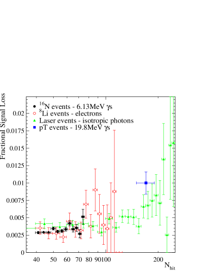
Figure 36: The signal loss measured from various calibrations sources as a function of the number of hit PMTs.

The figure shows that the signal loss inside the range of interest for measurements of events from ⁸B neutrinos (40-120 hits) is consistent with being flat. The same is true as a function of position within the D₂O volume and as a function of direction. The simplicity of these distributions allows the signal loss to be easily calculated for the different classes of events. Figure 36 also shows good agreement between the ¹⁶N and ⁸Li sources. This shows that the acceptance of the instrumental cuts does not depend upon the particle type, and therefore we can use the same acceptance for the electrons from the CC and ES reactions as we do for the neutrons from the NC reaction. We obtain the central value for the signal loss by fitting a flat distribution to the ¹⁶N and ⁸Li data. The best fit is found to be $(0.311\pm 0.007)\%$, where the uncertainty here is the statistical uncertainty in the fit.

The systematic uncertainty in this measurement comes from a number of sources. Uncertainties in calibrations of individual electronics channels were checked by re-running the signal-loss measurement with the calibration quality control flags turned off, leading to a one-sided systematic of $-0.021\%$. Deviations from the assumed flat distribution provide a systematic uncertainty of $\pm 0.028\%$. The biggest contributions to the systematic uncertainty arise from measurements of the stability of the signal loss as a function of time. The increase in signal loss due to faulty ADCs resulting in bad charge measurement on individual channels was measured, resulting in a correction of $(+0.027\pm 0.002)\%$. The performance of the instrumental cuts was monitored using periodic deployments of the ¹⁶N source. A systematic increase in signal loss is observed over time, resulting in a one-sided systematic uncertainty due to instability of $+0.11\%$. Combining these results in quadrature, the signal loss of the instrumental cuts is found to be $(0.34^{+0.11}_{-0.03})\%$.

IX.3.2 The Acceptance of the Reconstruction Algorithm

The reconstruction method described in Section V.4 has three distinct failure modes:

• The event may fail the figure-of-merit cuts, which test how well the event fits the hypothesis of a single Cherenkov electron. The figure-of-merit cuts act like high level cuts, and the acceptances of the two sets of cuts are correlated. For the purpose of cut acceptance, we therefore treat the figure-of-merit cuts together with the high level cuts.

• The reconstruction algorithm may not receive a good seed vertex. As described in Section V.4, the algorithm uses a seed vertex reconstructed using time information only. If the seed vertex lies outside the detector, or no vertex is returned then the reconstruction algorithm fails and the event is discarded.

• The event may fail during (negative-log) likelihood function minimization. This failure mode is relatively rare, being much less frequent than seed failure mode.

It is difficult to know exactly how reconstruction acceptance varies as a function of position and energy, because event location is, of course, not well known when reconstruction fails. Using scans taken with the ¹⁶N and ⁸Li sources, however, we find the signal loss decreases with increasing energy and increases sharply as events approach the acrylic vessel. The data from these scans do not allow us to make a measurement of the signal loss, but do allow us to place an upper limit of 0.3$\%$ for all classes of signal within the fiducial volume.

IX.3.3 The Acceptance of the High Level Cuts

Unlike the instrumental cuts, the high level cuts rely upon timing and hit pattern information only. For signal events these distributions can be reproduced much more reliably by simulation than can distributions such as the PMT charge distribution, and the Monte Carlo simulation can be used to integrate the distributions of cut acceptance for the high level cuts with the expected distributions for the three signals observed in SNO. Unlike the instrumental cuts and the reconstruction algorithm, the high level cuts have different acceptances for each of the three signals (CC, ES and NC).

The Monte Carlo simulation is used to calculate the acceptance for the high level cuts because we have no electron calibration source that is unaffected by its own hardware. The $\theta_{ij}$ cut in particular is sensitive to the amount of backward light. For electrons emitted by the ⁸Li source this backward light is blocked, giving a distorted $\theta_{ij}$ distribution. Furthermore, events initiated by $\gamma$-rays have a different $\theta_{ij}$ distribution from those initiated by electrons, because of the possibility that a second Compton-scattered electron could contribute light and produce a more isotropic hit pattern. Use of the Monte Carlo simulation allows these effects to be included.

Calibration data is not ignored, however. As shown in Figure 37a, the Monte Carlo simulation does not perfectly reproduce the measured signal loss for ¹⁶N data.

Figure 37: The signal loss of the high level cuts for ¹⁶N $\gamma$-rays from data and Monte Carlo simulation (a), and the ratio of the two distributions (b).

We see in the figure that the Monte Carlo simulation consistently overestimates the signal loss, an effect which is mainly due to the non-perfect reproduction of the $\theta_{ij}$ distribution by the simulation. To correct for this effect, a signal loss scale factor is calculated from the ratio of the data and Monte Carlo distributions (Fig. 37b). Above 40 hits the scale factor is independent of the number of hit PMTs. Below 40 hits the dominant contribution to the signal loss changes from the $\theta_{ij}$ cut to the reconstruction figure-of-merit cuts, resulting in a change of the scale factor. Very little of the signal data is below 40 hits, however, and this effect can therefore be ignored. The scale factor derived from a fit to the data above 40 hits is therefore used in the analysis. Using the scale factor, the signal loss of electrons within the analysis region is found to be $\sim$0.94$\%$ compared to 1.79$\%$ for neutrons.

There are three dominant contributions to the uncertainty of the signal loss due to high level cuts. The systematic uncertainty in the scale factor and the statistical uncertainty in the Monte Carlo simulated data sets contribute roughly equally to the uncertainty at the level of 0.05$\%$. There is a much larger contribution to the uncertainty due to the temporal stability of the cuts. Using the same ¹⁶N data set that was used to monitor the instrumental cuts, this contribution to the uncertainty of the signal loss is at the level of ${}^{+0.25}_{-0.11}\%$.

IX.3.4 Overall Cut Acceptance

As all three contributions to the signal loss (instrumental cuts, reconstruction failures, and high level cuts) are small and essentially uncorrelated, the combined signal loss can be found by direct addition of the individual contributions. Calculation of the uncertainty has a complication as the same data set was used to measure many of the uncertainties due to stability. To account for this correlation these uncertainties are added linearly and combined with the remaining uncertainties in quadrature. The signal loss due to reconstruction was not measured; instead an upper limit was placed at 0.3$\%$ and it was included as a contribution of $0.15\pm 0.15\%$ to the overall signal loss uncertainty. The final signal loss measurement for the three signals are therefore:

$${\rm CC} (1.43^{+0.39}_{-0.21})\%$$

$${\rm ES} (1.46^{+0.40}_{-0.21})\%$$

$${\rm Neutrons} (2.28^{+0.41}_{-0.23})\%$$

IX.4 Target

IX.4.1 Numbers of Deuterons

The neutrino interaction rate depends on the number of targets within the fiducial volume selected, which, in turn, depends on the isotopic enrichment and density. The fiducial volume used, a 550-cm radius sphere, is defined by event reconstruction supported by calibration. A second volume is defined by the acrylic vessel (AV) sphere itself, which provides both a geometrically defined fiducial volume against which reconstruction can be checked, and a precisely known volume of D₂O that can be compared to the directly weighed inventory.

We determined the density of the heavy water directly in a surface laboratory at the SNO site at temperatures in the range of $17^{\circ}$ - $21^{\circ}$ C. We corrected to $11^{\circ}$ C using published tabulations, as the actual operating temperature was $11.5^{\circ}$ C, at which temperature the density differs negligibly. Our measured density for the heavy water is 1.10555(10) g cm^-3, and we add a correction for compressibility which raises the value to 1.10563(10), as the mean gauge pressure underground at SNO is 0.15 MPa.

The surveyed dimensions of the vessel, deviations from a spherical shape, corrections for swelling and distortion, temperature, the measured D₂O specific gravity and the compressibility give a calculated mass that may be compared to the weighed inventory. Table 14 summarizes the volumes, densities, and masses of the various components of the detector. The calculated mass of the D₂O has an uncertainty of roughly 0.3%, dominated by geometrical uncertainties. The volumetrically determined mass exceeds the inventory mass by 828 kg, a discrepancy well within the estimated uncertainty.

Table 14: Heavy water inventory.

Quantity
Temperature	$11.5^{\circ}$	C
Density at 1 atm and $11.5^{\circ}$ C	1.10555	g cm-3
Mean gauge pressure in SNO	0.15	MPa
Isothermal Compressibility	4.59 x 10-4	MPa-1
Corrected density	1.10563	g cm-3
Vessel radius as surveyed	600.5(6)	cm
Vessel radius in service	600.54(61)	cm
Calculated mass in sphere	1003049	kg
Calculated mass in neck	8963	kg

The number of target deuterons also depends on the isotopic abundance of the heavy water. Because neutron transport and detection are also sensitive to the abundances, the isotopic mixture determines the characteristic radial profile for capture events as well as the proportions of neutrons capturing on each isotope. The enrichment process also affects the oxygen isotope abundances. The precise abundances of these isotopes are relevant for corrections for the substantial neutron-capture cross section on ¹⁷O and for neutrino charged-current interactions on ¹⁸O.

The hydrogen isotope mass fractions are determined by Fourier Transform Infrared (FTIR) Spectroscopy on samples taken from the detector volume recirculation path. The mean measured isotopic abundance for deuterium between October 1999 and March 2000 was 99.9176% with a standard deviation of 0.0023 based on 29 samples. The corresponding number fraction is 0.999084, which is the value we use in this article. When measurements through November 2001 are included, the resulting deuterium mass fraction is $99.9168\pm 0.0021$%. The corresponding number fraction is $99.9076\pm 0.0021$%. The largest uncertainty in the absolute isotopic measurement comes from the accuracy of the standard, $\pm$0.01%.

The ^16,17,18O isotope number fractions were determined by analytic chemistry measurements made outside the SNO collaboration. Three independent techniques were applied to three separate heavy-water samples. Nuclear magnetic resonance 17nmr as well as infrared laser spectrometry was used to extract direct measurements of the ¹⁷O and ¹⁸O number fractions kerstel . CO₂-water equilibration was used to measure the ¹⁸O abundance co2-h2o . Recommended values are obtained by taking weighted averages over the independent measurements. All values are presented in Table 15.

The values given for the oxygen isotopes are very different from the ones in NIM as a result of the new measurements. A systematic error associated with an ion-mass degeneracy is suspected to have influenced the earlier measurement.

The number of molecules in a heavy water target of mass $M$ is

$$N_{M}=\frac{M}{2m_{D}f_{D}+2m_{H}(1-f_{D})+m_{17}f_{17}+m_{18}f_{18}+m_{16}(1-f_{17}-f_{18})},$$ (47)

where $f_{D}$, $f_{17}$, and $f_{18}$ are the atom-fraction isotopic abundances of deuterium, ¹⁷O, and ¹⁸O, respectively, and $m_{i}$ is the atomic mass of oxygen isotope $i$. There are 2$N_{M}f_{D}$ deuterons in this target of mass $M$, so from Eq. 47 and the isotopic enrichment data there are

$$N_{D}=6.0082(62)\times 10^{31}$$

deuterons in 1000 tonnes of SNO heavy water. The error is from the uncertainty in the deuteron isotopic abundance (0.0023% (stat.), 0.01% (syst.)). For a given fiducial volume the error on the density of SNO heavy water (0.009%) must be included.

The elastic scattering reaction similarly depends on the volume and density. The number of electrons per mass $M$ of heavy water is 10$N_{M}$. There are thus $30.0684\times 10^{31}$ electrons per 1000 tonnes. The dependence on composition is very weak.

Table 15: SNO heavy water oxygen isotope number fractions.

Measurement Technique	18O (%)	17O (%)
IR Laser Spectrometry	0.33$\pm$0.03	0.049$\pm$0.005
CO2-water Equilibration	0.320$\pm$0.006	0.0486$\pm$0.0009
17O NMR	0.311$\pm$0.004	0.0479$\pm$0.0006
Recommended Values	0.320$\pm$0.003	0.0485$\pm$0.0005

Table 16: Allowed nuclear matrix elements $|$M$|^{2}$ = BGT + BF and the resulting cross sections, averaged over an undistorted ⁸B neutrino flux. Here, BGT stands for the Gamow-Teller part of the matrix element, and BF the Fermi part.

Target	$E_{f}$(MeV)	Q(MeV)	BGT	BF	$\sigma(^{8}$B)
					(10-42 cm2)
18O	0.0	-1.655	5.12		4.14
	1.04	-2.695		2.0	1.11
	1.70	-3.355	0.21		0.103
	Total				5.35(5)
17O	0.0	-2.761	1.69	1.0	1.53(1)
2H	0.0	-1.442			1.15(4)

IX.4.2 Other Isotopes

We include the terms for ¹⁷O and ¹⁸O in Equation 47 because these rare isotopes of oxygen play a role similar to deuterium in their CC interactions with ⁸B neutrinos. Most of the cross section is due to a super-allowed transition to the ground state, but, unlike deuterium, the final states are narrow and stable to nucleon emission. The interaction cross sections have been calculated in Haxton and are summarized in Table  16. Substituting the measured ¹⁷O and ¹⁸O abundances gives the correction to the deuterium CC rate as 1.0078(10). The main uncertainty of 0.001 in this small correction factor comes from the variation in Q-value from 1.4 to 3.3 MeV; the uncertainties in the isotopic abundances and the matrix elements contribute very little (for pure Fermi and ground-state Gamow-Teller matrix elements the uncertainties are 1% or less). The angular distribution is slightly influenced. For reactions on ¹⁸O it is essentially flat while for ¹⁷O it is also weak but slightly forward peaked Haxton .

IX.5 Neutron Capture and Detection Efficiency

Several factors prevent the neutron detection efficiency from being unity. First, the finite D₂O volume means that some of the neutrons liberated from deuterium can escape the heavy water and then capture on hydrogen in the acrylic vessel or light water shield. Second, free neutrons in the heavy water also have a non-zero probability of being captured on nuclei other than deuterium, such as hydrogen, ¹⁶O, ¹⁷O, and ¹⁸O. Lastly, our energy threshold and fiducial volume cuts remove a large fraction of the 6.25 MeV capture $\gamma$-rays from the final data set.

We have measured the neutron capture efficiency by deploying a ²⁵²Cf source at various positions throughout the heavy water volume. These “point-source” calibrations have been employed, together with Monte Carlo simulation and an analytic diffusion model, to extract the capture efficiency and its uncertainty relevant to a source of neutrons uniformly distributed throughout the heavy water volume. As discussed in Section IV.4, our Monte Carlo simulation of neutron propagation and capture is based upon Los Alamos National Laboratory’s MCNP code. An analytic model for neutron transport in SNO has been derived that relates the macroscopic quantities of interest such as absorption, diffusion length, and lifetime, to the microscopic quantities such as isotopic abundances and capture cross-sections.

The ²⁵²Cf source created fission $\gamma$s and $\beta$s as well as neutrons. These can contaminate the 6.25 MeV capture-gamma distribution of interest. Since these backgrounds have a mean path length in D₂O that is short in comparison to the mean neutron capture distance of about 120 cm, they were avoided by requiring events to reconstruct more than 80 cm from the source. The loss of efficiency by invoking this cut is determined via Monte Carlo simulation which accurately reproduces the radial profile of neutron captures in the D₂O. An example is shown in Figure 38

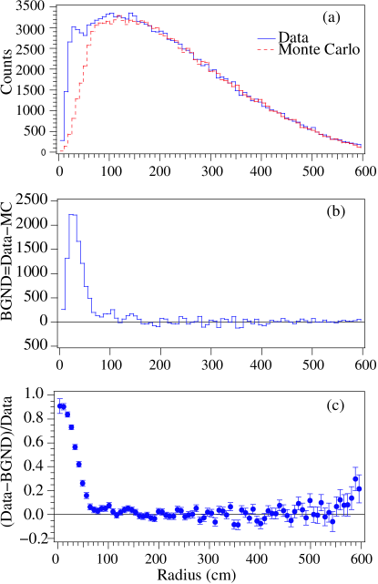
Figure 38: Radial profile of neutron captures for ²⁵²Cf source deployed at the center of the detector, compared to Monte Carlo simulation of the source. In (a) we compare the raw data distribution of events to the Monte Carlo simulation, and we see that the data has an excess due to the associated $\gamma$s and $\beta$s produced by the source. The difference between the two curves is shown in (b), and the ratio of (b) to the data shown in (c). The drop off around 80 cm motivates the cut to remove the non-neutron events in the calculation of the efficiency.

for the radial profile obtained with the ²⁵²Cf source deployed near the center of the heavy water volume. The associated 6.25 MeV gamma energy distribution is shown in Figure 39.

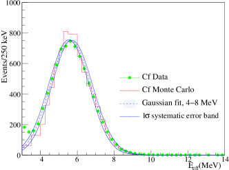
Figure 39: Energy spectrum of $\gamma$-rays from neutron capture for deployment of ²⁵²Cf source at the center of the detector.

As can be seen in Fig. 39, the 6.25 MeV gamma energy distribution is well described by a Gaussian distribution. The number of neutrons is determined from this distribution by fitting the centroid and width to the calibration data above $T_{\rm eff}=5.0$ MeV and extrapolating the fit to zero energy. In this way, correlated uncertainties associated with the absolute energy scale and resolution are avoided. After correcting for the radial cut mentioned above we obtain the total number of neutrons captured on deuterium for the ²⁵²Cf at a given position in the detector. By knowing the livetime for a particular calibration run and the absolute neutron yield of the ²⁵²Cf source we can determine the capture efficiency for a point source deployed at a specific location or radius in the detector. Figure 40 shows the results from this exercise for a set of ²⁵²Cf calibration scans throughout the detector.

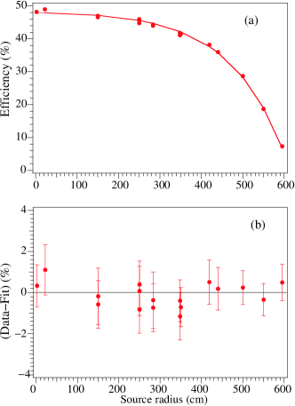
Figure 40: Capture efficiency for neutrons from ²⁵²Cf source at several locations throughout the detector volume. In (a) we compare the measurements (filled dots) to the analytic calculation (solid curve), and in (b) the difference between them.

Fig. 40 yields the absolute capture efficiency for neutrons on deuterium that reconstruct within the D₂O volume when their origin is a ²⁵²Cf source at a specific position in the detector. We need to exploit this information to deduce the capture efficiency of interest, namely the volume-weighted sum of neutrons captured from a source uniformly distributed throughout the heavy water volume. To do so we require a function to interpolate between the discrete calibration points which can then be fed into the volume-weighted integral of interest. We have developed an analytic neutron diffusion model that serves this purpose well. The smooth curve in Fig. 40 arises from a fit to the calibration data using a two-parameter model predicting the radial profile for point-neutron sources in the detector according to:

$$\epsilon(R)=\epsilon_{0}[1-F_{\rm escape}(R)]$$ (48)

where

$$F_{\rm escape}(R) = \frac{R_{AV}}{R}\frac{\sinh(\frac{R}{l})}{\sinh(\frac{R_{e}}{l})}[\cosh(\frac{R_{e}-R_{AV}}{l})$$

$$+ \frac{l}{R_{AV}}\sinh(\frac{R_{e}-R_{AV}}{l})].$$

In Equations 48 and IX.5, $R$ is the position of the point-source calibration data, measured in cm. The leading scale factor ($\epsilon_{0}$) in Eq. 48 describes the capture efficiency for the case where the SNO heavy water volume is infinite in extent. In Eq. IX.5, $R_{AV}$ is the 600 cm radius of the heavy water volume, and $R_{e}$ the radius at which a perfect absorber would need to be placed to represent the effects of the acrylic and light water (roughly 15 cm beyond the inner surface of the acrylic vessel).

The escape of neutrons that arises due to the finite detector radius of $R_{AV}=600$ cm and the non-zero diffusion length ($l$) explains the drop-off in efficiency for a source closer to the AV. A fit to the data yields:

$$\epsilon_{0}=0.499\pm 0.010$$

and

$$l=109.4\pm 4.8~{}{\rm cm}.$$

The same analytic diffusion model can be used to predict the capture efficiency for a source of neutrons uniformly distributed throughout the heavy water volume. It is described using the same two parameters after integrating Eq. IX.5 out to a fiducial volume of radius $R_{f}$:

$$F^{\rm NC}_{\rm escape} = \frac{1}{R_{AV}^{3}}[R_{f}^{3}-3l[R_{f}\cosh(\frac{R_{f}}{l})-l\sinh(\frac{R_{f}}{l})]$$

$$\times\frac{[R\cosh(\frac{R_{e}-R_{AV}}{l})+l\sinh(\frac{R_{e}-R_{AV}}{l})]}{\sinh(\frac{R_{e}}{l})}]$$

Using the parameters constrained in the fit to the point-source data we deduce a NC neutron capture efficiency of: $0.299\pm 0.011$.

This efficiency corresponds to neutrons capturing on deuterium with an effective detector energy threshold of zero and a full fiducial volume of 600 cm. Monte Carlo simulation was used to determine the reduction in efficiency relevant to our analysis threshold of $T_{\rm eff}$=5.0 MeV and 550 cm fiducial volume. In this case, the neutron detection efficiency relevant to our analysis is $0.1438\pm 0.0053$, with the breakdown of statistical and systematic uncertainties outlined in Table 17.

Table 17: Statistical and systematic uncertainties on the neutron capture measurement.

Contribution	Uncertainty (%)
Energy Distribution	1.74
Source Standard	2.20
Source Exclusion	0.86
Source Position	0.95
Total Systematic Uncertainty	3.09
Statistics of 252Cf data	1.97
Total Uncertainty	3.68

For verification of this ‘direct counting’ method, we used a multiplicity analysis that compared the number of neutrons detected per ²⁵²Cf decay to expectations based on knowledge of the primary decay neutron multiplicity and Monte Carlo simulation. The results of the multiplicity analysis were in excellent agreement with the direct counting method described above, albeit with somewhat larger uncertainties.

X Final Flux Measurements

The cuts described in Section V, including the energy threshold of $T_{\rm eff}=5.0$ MeV and the fiducial volume restriction of $R_{\rm fit}<550$ cm, constitute our primary event selection criteria. After application of these cuts to the full data set, 2928 candidate neutrino events remain, and the signal extraction fit is performed on this event sample.

As a consistency check, the signal extraction fit was repeated using the total number of hit tubes ($N_{\rm hit}$) as the estimate of event energy rather than the prompt-time reconstructed energy described in Section V.5. For this $N_{\rm hit}$-based analysis the energy threshold cut was replaced by a cut of $N_{\rm hit}\geq 45$, chosen to give a total number of events in the final data sample that matched the number using the cut on effective energy. We further explored the dependence on fiducial volume by performing fits to data that used both tighter and looser radial cuts, including out into the H₂O volume.

As discussed in Section VIII, in our primary approach to signal extraction, we used pdfs generated by the Monte Carlo. For verification, we also performed an extraction using pdfs generated by analytic parameterizations of the response, as described in Section VIII.5. The analytic approach was also used for our estimation of the neutrino mixing parameters, as discussed in Appendix XIV.

This section will concentrate on the derivation of the flux results from the Phase I NC paper SNO Collaboration (2002a), but in Section X.8 we will comment on the high energy threshold analysis in the ES-CC paper SNO Collaboration (2001). The Day-Night asymmetry measurement will be discussed in Section XI.

X.1 Spectrum-Constrained Fluxes

The primary signal extraction was performed as described in Section VIII, with three signal pdfs (plus background pdfs) in $T_{\rm eff},R^{3}$, and $\cos\theta_{\odot}$, with the CC and ES event energy spectra constrained to follow their expected shapes for an undistorted ⁸B $\nu$ spectrum ortiz . The raw numbers of extracted signal events of each type are given in Table 18. The errors quoted here are symmetric parabolic errors as calculated by MINUIT’s HESSE routine MINUIT , and are very similar to the MINOS asymmetric errors. Table 19 shows the full correlation matrix for the signals obtained in the extraction process.

Table 18: Extracted numbers of CC, ES, and NC events in the full D₂O data set, with a ⁸B spectral constraint on the CC and ES spectra. Errors are statistical only. Note that the backgrounds discussed in Section VII have been subtracted off in the manner discussed in Section VIII.

Signal	Events
CC	$1967.71\pm 61.36$
ES	$263.64\pm 25.68$
NC	$576.53\pm 48.82$

Table 19: Statistical correlation matrix between CC, ES, and NC signals from the signal extraction with a ⁸B shape constraint.

	CC	ES	NC
CC	1.000	-0.162	-0.520
ES	-0.162	1.000	-0.105
NC	-0.520	-0.105	1.000

The raw number of extracted events of each signal type may be converted to a flux through Equation 50, which yields a flux in units of $10^{6}$ neutrinos/cm²/sec:

$$\phi_{i}=\frac{N_{i}}{N_{\rm MC}}\cdot L\cdot\frac{1}{\epsilon_{\rm cuts}}\cdot f_{{\rm O}}\cdot{\cal E}\cdot X$$ (50)

The various quantities are defined as:

$N_{i}$:
Number of extracted events for a given signal type $i$, as given in Table 18

$N_{\rm MC}$:
Number of Monte Carlo events inside the signal region, for a total ⁸B flux of $1\times 10^{6}$/cm²/sec. The number of events we generated was 50 times the BPB2000 SSM prediction of $5.15\times 10^{6}\nu~{}{\rm cm}^{-2}{\rm s}^{-1}$ Bahcall et al. (2001).

L:
Livetime correction factor. This correction accounts for detector deadtime due to the imposition of time-correlated cuts (such as those that remove muon follower events).

$\epsilon_{\rm cuts}$:
Acceptance of low and high level cuts, as described in Sections IX.3.1 and IX.3.3, that are not applied to the Monte Carlo simulation.

$f_{{\rm O}}$:
A correction to the CC flux due to CC neutrino interactions on ¹⁷O and ¹⁸O, as described in Section IX.4.2. These interactions are not modeled in the Monte Carlo simulation. This correction is applicable only to the CC flux.

${\cal E}$:
Correction for eccentricity of the Earth’s orbit, which was not included in the Monte Carlo generation.

$X$: Minor corrections to the neutrino cross sections assumed in the Monte Carlo simulation. For the CC and NC fluxes, this is a combination of the $g_{A}$ correction to the Butler, Chen, and Kong (BCK) cross section BCK , a downward revision of the NSGK cross section NSGK , and radiative corrections of Kurylov et al. kmv . See Section IV.1 for further details.

Table 20 contains the values of the flux correction factors used for each signal.

Table 20: Flux correction factors for converting event totals to fluxes. The final entry (“Total”) is the product of all the corrections which are applied to the ratio $N_{i}/MC$ to convert it into a flux in units of $10^{6}$ neutrino/cm²/sec.

Correction	Symbol	CC	ES	NC
Livetime	Total/Corrected	312.93/306.39	312.93/306.39	312.93/306.39
Cut efficiency	$\epsilon_{\rm cuts}$	$0.986^{+0.004}_{-0.002}$	$0.985^{+0.004}_{-0.002}$	$0.977^{+0.004}_{-0.002}$
17O and 18O correction	$f_{{\rm O}}$	1/1.00793	1	1
Eccentricity correction	${\cal E}$	1/1.0069	1/1.0069	1/1.0069
Cross section correction	X	1/1.0162	1.02	1/1.0112
Total Correction Factor		1.0043	1.0500	1.0267
Number of events	$N$	$1967.71\pm 61.36$	$263.64\pm 25.68$	$576.53\pm 48.82$
MC Prediction (for $10^{6}$ $\nu~{}{\rm cm}^{-2}{\rm s}^{-1}$)	$N_{\rm MC}$	1120.48	115.83	116.23

With all of these corrections applied, the extracted signal fluxes are (statistical errors only):

$\phi_{CC}=1.76^{+0.06}_{-0.05}\times 10^{6}$ cm^-2 s^-1

$\phi_{ES}=2.39^{+0.24}_{-0.23}\times 10^{6}$ cm^-2 s^-1

$\phi_{NC}=5.09^{+0.44}_{-0.43}\times 10^{6}$ cm^-2 s^-1

The physical interpretation of the “flux” for each interaction type is that it is the equivalent flux of ⁸B $\nu_{e}$s produced from an undistorted energy spectrum that would yield the same number of events inside the signal region from that interaction as was seen in the data set.

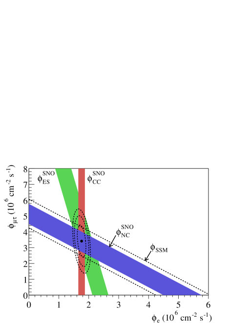
Figure 41: Flux of ⁸B solar neutrinos which are $\mu$ or $\tau$ flavor vs flux of electron neutrinos deduced from the three neutrino reactions in SNO. The diagonal bands show the total ⁸B flux as predicted by the BP2000 SSM Bahcall et al. (2001) (dashed lines) and that measured with the NC reaction in SNO (solid band). The intercepts of these bands with the axes represent the $\pm 1\sigma$ errors. The bands intersect at the fit values for $\phi_{e}$ and $\phi_{\mu\tau}$, indicating that the combined flux results are consistent with neutrino flavor transformation with no distortion in the ⁸B neutrino energy spectrum.

The inequality of the CC, ES, and NC fluxes provides strong evidence for a non-$\nu_{e}$ component to the ⁸B neutrino flux. Figure 41 shows the constraints on the flux of $\nu_{e}$ versus the combined $\nu_{\mu}$ and $\nu_{\tau}$ fluxes derived from the CC, ES, and NC rates. Together the three rates are inconsistent with the hypothesis that the ⁸B flux consists solely of $\nu_{e}$s, but are consistent with an admixture consisting of $\sim 1/3~{}\nu_{e}$ and $2/3~{}\nu_{\mu}$ and/or $\nu_{\tau}$.

X.1.1 Goodness of Fit

The signal extraction is done by a maximum likelihood fit which does not readily yield an absolute goodness-of-fit parameter. One means of investigating the goodness of fit of the signal extraction is to calculate the $\chi^{2}$ of the radial, energy, and angular marginal distributions between the data and the best-fit sum of the weighted pdfs. This $\chi^{2}$ is defined as:

$$\chi^{2}=\sum_{i=1}^{bins}(R_{\rm DATA}(i)-R_{\rm pdfs}(i))^{2}/R_{\rm DATA}$$ (51)

Here, $R_{\rm DATA}(i)$ is the number of counts in the $i$th bin of the data ($R$ may be a histogram in energy, angle, or radius). $R_{\rm pdfs}(i)$ is the predicted number of counts in the $i$th bin, found by weighting each signal pdf by the number of fitted events and summing these renormalized pdfs. This $\chi^{2}$ calculation does not account for systematic uncertainties.

Table 21: $\chi^{2}$ values between data and fit for the energy, radial, and angular distributions, for the fit using the constraint that the effective kinetic energy spectrum results from an undistorted ⁸B shape.

Distribution	Number of Bins	$\chi^{2}$
Energy	42	34.58
Radius	30	39.28
Angle	30	19.85

Table 21 shows the $\chi^{2}$ values for the fits using the constraint that the effective kinetic energy spectrum results from an undistorted ⁸B shape. In each case the $\chi^{2}$ per degree of freedom is close to one. One must be cautious in interpreting these results. Although the signal extraction fit has 3 free parameters, one should not subtract 3 degrees of freedom for each $\chi^{2}$, since the fit is a global fit to all three distributions. Furthermore, the actual signal extraction is a fit to the three-dimensional data distribution, whereas the $\chi^{2}$s are calculated with the marginal distributions. These “$\chi^{2}$” values demonstrate that the weighted sum of the signal pdfs provides a good match to the marginal energy, radial, and angular distributions.

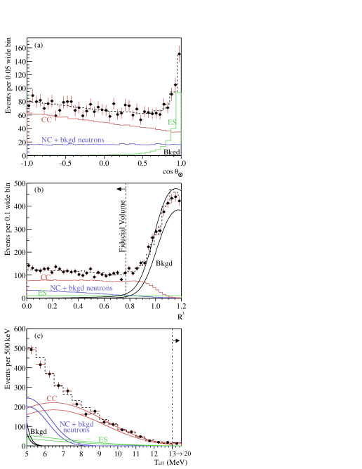
Figure 42: (a) Distribution of $\cos\theta_{\odot}$ for $R_{\rm fit}\leq 550$ cm. (b) Distribution of the radial variable $R^{3}=(R_{\rm fit}/R_{AV})^{3}$. (c) Kinetic energy for $R_{\rm fit}\leq 550$ cm. Also shown are the Monte Carlo predictions for CC, ES and NC + background neutron events scaled to the fit results, and the calculated spectrum of $\beta$-$\gamma$ background (Bkgd) events. The dashed lines represent the summed components, and the bands show $\pm 1\sigma$ statistical uncertainties from the signal extraction fit. All distributions are for events with $T_{\rm eff}$$\geq$5 MeV.

Figure 42 shows the marginal radial, angular, and energy distributions of the data along with Monte Carlo predictions for CC, ES and NC + background neutron events, scaled by the fit results.

X.1.2 Results of Fitting for Flavor Content

An alternative approach to doing a null hypothesis test for neutrino flavor conversion, as discussed in Section VIII.4, is to fit for the fluxes of $\nu_{e}$ and $\nu_{\mu\tau}$ directly. This is a simple change of variables to the standard signal extraction. Fitting for the flavor content instead of the 3 signal fluxes, we find:

$\phi(\nu_{e})=1.76\pm 0.05\times 10^{6}$ cm^-2 s^-1

$\phi(\nu_{\mu\tau})=3.41\pm 0.45\times 10^{6}$ cm^-2 s^-1

The statistical correlation coefficient between these values is $-0.678$. We will discuss the statistical significance of the non-zero $\phi(\nu_{\mu\tau})$ flux in Section X.6 where we include the systematic uncertainties.

X.2 Sensitivity of Results to Choice of Energy Threshold, Fiducial Volume, and Energy Estimator

To verify the stability of the extracted flux results, we repeated the signal extraction and flux calculations with different choices of fiducial volume, energy threshold, and energy estimator. These variations included restricting the fiducial volume to 500 cm and 450 cm, extending the fiducial volume to 620 cm and including external background pdfs, raising the energy threshold to $T_{\rm eff}>5.5$ MeV, and using the $N_{\rm hit}$ variable instead of the calibrated energy in MeV as the energy variable in the signal extraction. All of these variations produced fluxes that agreed with the primary analysis within the expected uncertainties.

X.3 Inclusion of Additional $(\alpha,n)$ Neutrons from the Acrylic

As discussed in Section VII.6, our estimates of the contribution from neutrons produced by radioactivity external to the heavy water volume are based on measurements of the U and Th content of the acrylic and light water, and on expectations for the resultant number of photodisintegration neutrons that pass our energy threshold and fiducial volume cuts. In addition to these neutrons, $(\alpha,n)$ reactions on nuclei in the acrylic vessel are also a source of ‘external’ neutrons, but are not included in our overall background estimates that lead to our neutrino flux measurements.

To determine the effects of the inclusion of this background, subsequent to the publication of the results in the NC paper SNO Collaboration (2002a) we performed a signal extraction fit in which we allowed the amplitude of the external neutron background to float. The results of this fit with a floating external neutron background are consistent with the results with the background level constrained to the value in Table 9 to within uncertainties. Their inclusion would thus lead to a small increase in our overall quoted systematic uncertainty. In a future publication we will include updates to the flux measurements contained in this article that will explicitly incorporate the (minor) effects of this background.

X.4 Spectrum-Unconstrained Flux Results

One can produce an “unconstrained” NC flux result, requiring no assumptions about the CC energy spectrum, by doing an extraction based only upon $R^{3}$ and $\cos\theta_{\odot}$. This can be easily implemented as a binned maximum likelihood fitter by setting the number of energy bins in the pdfs to 1. The resulting fit is equivalent to performing an unconstrained signal extraction with a single CC spectral bin.

Table 22 shows the results of the unconstrained fit on the data set. Table 23 shows the correlation matrix. The anticorrelation between the CC and NC signals is nearly -100%.

Table 22: Extracted numbers of events and fluxes for SNO’s full D₂O data set, derived with no constraint on the shapes of the CC and ES energy spectra.Note that the backgrounds discussed in Section VII have been subtracted off in the manner discussed in Section VIII.

Signal	Events	Flux
CC	$1833.38\pm 173.76$	$1.64\pm 0.16\times 10^{6}$
ES	$253.21\pm 26.64$	$2.30\pm 0.24\times 10^{6}$
NC	$717.71\pm 176.97$	$6.42\pm 1.57\times 10^{6}$

Table 23: Correlation Matrix, Unconstrained Signal Extraction for NC flux, $5<T<19.5$ MeV

	CC	ES	NC
CC	1.000	0.208	-0.950
ES	0.208	1.000	-0.297
NC	-0.950	-0.297	1.000

X.5 Systematic Uncertainties

Three separate classes of systematic uncertainties need to be propagated to the final flux calculation: uncertainties on the background estimates, uncertainties that affect only the flux normalization, and uncertainties on the model used to generate the pdfs. The last of these can affect both the pdf shapes and the overall normalization. The handling of background uncertainties is described in Section VIII.3, and uncertainties on the backgrounds themselves are discussed in Section VII and summarized in Table 9. Uncertainties that affect only the overall flux normalization—uncertainties on acceptance loss of the applied cuts, on neutron capture efficiency, and on the D₂O target—are applied directly to the final flux calculation. Section IX discussed these normalization uncertainties.

Systematic uncertainties that affect both the shapes of the pdfs and the overall normalization are propagated to the final flux measurements by shifting the radius, angle, or energy of the Monte Carlo events used to form the signal pdfs, or, for the extraction using analytic pdfs described in Section VIII.5, by varying the analytic detector response parameters within their uncertainties. These uncertainties are each discussed in detail in Section VI, and include uncertainties on the energy scale, resolution, and non-linearity; vertex accuracy and resolution; and angular resolution.

The effect of the shape-related systematic uncertainties is determined by separately shifting the value of each affected parameter by its $\pm 1\sigma$ uncertainty, and then repeating the signal extraction and flux calculation with the shifted pdfs. For example, to model the $\pm 1.2\%$ systematic uncertainty in the overall energy scale, the energies of all Monte Carlo events are first shifted upward by 1.2%, a set of perturbed pdfs is generated, and these perturbed pdfs are used to perform a signal extraction and flux calculation. Then a similar set of perturbed pdfs with the energies shifted by $-l$1.2% is generated and used. For uncertainties affecting resolutions, the resolution is ‘shifted’ by convolving the pdfs with a Gaussian distribution. The Gaussian convolution smears the pdfs, thus acting like a broadened resolution function.

The perturbations to the pdf shapes are only applied to the signal pdfs, not to background pdfs. As described in Section VIII.3, the amplitudes of the background pdfs are themselves varied between their $\pm 1\sigma$ limits, and these uncertainties are typically so large (30-50%) that they dominate over any shape-related uncertainty. We have studied a number of perturbations on the background pdf shapes themselves, such as varying their radial profiles over wide ranges, from steeply sloped to almost flat, and have seen negligible flux changes. Generally speaking, the background pdfs fall so rapidly in energy, that including them in the fit almost always tends to reduce the number of NC events in the lowest energy bin.

For the constrained fit in which one fits for the CC, ES, and NC fluxes simultaneously, the systematic uncertainties are themselves correlated between the different signals. For the fit to the flavor content ($\phi(\nu_{e})$ and $\phi(\nu_{\mu\tau})$ described in Section VIII.4, these correlations simplified—while there are correlations between the electron and muon or tau neutrino fluxes, the null hypothesis test is a simple one-variable test on $\phi(\nu_{\mu\tau})$.

Table 24: Systematic uncertainties on the fluxes for the shape-constrained signal extraction. The relative ordering of the upper and lower uncertainties on the fluxes indicates that a systematic is correlated between two fluxes (same sign ordering) or anticorrelated (reverse sign ordering). The ‘Experimental uncertainty’ listed in the bottom row refers to the contribution from systematic uncertainties propagated through the signal extraction process, but does not include normalization or efficiency uncertainties, or theoretical uncertainties.

Source	CC Uncertainty.	NC Uncertainty	ES Uncertainty	$\phi_{e}$ Uncertainty	$\phi_{\mu\tau}$ Uncertainty
	(percent)	(percent)	(percent)	(percent)	(percent)
Energy scale	-4.2,+4.3	+6.1,-6.2	-3.1,+3	+10.3,-10.4
Energy resolution	-0.9,+0.0	+4.4,-0.0	-0.4,+0.0	-1.0,+0.0	+6.8, -0.0
Energy non-linearity	-0.1,+0.1	+0.4,-0.4	0.0	-0.1,+0.1	+0.6,-0.6
Vertex resolution	0.0	-0.1,+0.1	0.0	0.0	-0.2,+0.2
Vertex accuracy	-2.8,+2.9	-1.8,+1.8	-2.9,+2.9	-2.8,+2.9	-1.4,+1.4
Angular resolution	-0.2,+0.2	-0.3,+0.3	+2.1,-2.0	-0.1,+0.1	+0.3,-0.3
Internal source pd	0.0	-1.5,+1.6	0.0	0.0	-2.0,+2.2
External source pd	-0.1,+0.1	-1.0,+1.0	-0.1,+0.1	-0.1,+0.1	$\pm 1.4$
D2O $\beta$-$\gamma$	-0.1,+0.2	+1.2,-2.6	+0.5,-0.2	-0.1,+0.3	+1.7,-3.7
H2O $\beta$-$\gamma$	0.0	-0.2,+0.4	-0.1,+0.2	0.0	-0.2,+0.6
AV $\beta$-$\gamma$	0.0	-0.2,+0.2	-0.1,+0.1	0.0	-0.3,+0.3
PMT $\beta$-$\gamma$	-0.1,+0.1	+1.6,-2.1	+0.1,-0.1	-0.1,+0.1	+2.2,-3.0
Neutron capture	0.0	-4.0,+3.6	0.0	-0.1,+0.1	-5.8,+5.2
Cut acceptance	-0.2,+0.4	-0.2,+0.4	-0.2,+0.4	-0.2,+0.4	-0.2,+0.4
Experimental uncertainty	-5.2,+5.2	-8.5,+9.1	-4.8,+5.0	-5.3,+5.4	-13.2,+14.1
Cross section	$\pm 1.8$	$\pm 1.3$	—	—	$\pm 1.4$

Table 24 contains the systematic uncertainties on the three signals and on the flavor-dependent fluxes. Several things should be noted. First, separate positive and negative errors are given for each systematic. The ordering of signs on the systematic uncertainties between columns indicates the sign of the correlation between the signals in each column: same-sign ordering indicates correlations between elements, while opposite sign ordering indicates anti-correlations.

Table 25 gives the systematic errors for the unconstrained analysis (fitting only with $R^{3}$ and $\cos\theta_{\odot}$ between $5<T_{\rm eff}<19.5$ MeV). The systematics must be propagated separately for this fit, since the sensitivity to each systematic has now changed. For example, since the radial profile of the signals is the dominant factor for separating CC from NC events, systematics that affect the radial profiles, such as radial shift or the amplitude of the AV $\beta-\gamma$ background (which has a steeply changing radial profile), will have a much larger effect than they have for the constrained signal extraction.

Table 25: Systematic uncertainties on the fluxes for the shape-unconstrained signal extraction. The relative ordering of the upper and lower uncertainties on the fluxes indicates that a systematic is correlated between two fluxes (same sign ordering) or anticorrelated (reverse sign ordering). The ‘Experimental uncertainty’ listed in the bottom row refers to the contribution from systematic uncertainties propagated through the signal extraction process, but does not include normalization or efficiency uncertainties, or theoretical uncertainties.

Source	CC Uncertainty.	NC Uncertainty	ES Uncertainty
	(percent)	(percent)	(percent)
Energy scale	-1.3,+1.4	-3.7,+4.2	-2.2,+2.3
Energy resolution	-0.0,+0.3	-0.0,+0.2	0.0
Energy non-linearity	0.0	0.0	0.0
Vertex resolution	-0.4,+0.5	+0.9,-0.8	-0.1,+0.1
Vertex accuracy	-0.8,+1.0	-5.9,+5.6	-2.3,+2.3
Angular resolution	-0.2,+0.3	-1.2,+1.1	+2.2,-2.0
Internal source pd	0.0	-1.1,+1.2	0.0
External source pd	-1.0,+1.0	+1.1,-1.1	-0.3,+0.3
D2O $\beta$-$\gamma$	-0.6,+0.3	-0.3,+0.1	-0.2,+0.1
H2O $\beta$-$\gamma$	-0.9,+2.1	+1.6,-3.6	-0.2,+0.7
AV $\beta$-$\gamma$	-1.2,+0.9	+2.1,-1.6	-0.4,+0.3
PMT $\beta$-$\gamma$	-1.0,+0.7	+0.8,-0.6	-0.3,+0.3
Neutron capture	-0.1,+0.1	-3.6,+3.4	0.0
Cut acceptance	-0.2,+0.4	-0.2,+0.4	-0.2,+0.4
Experimental uncertainty	-2.7,+3.2	-9.1,+8.6	-4.0,+4.2
Cross section	$\pm 1.8$	$\pm 1.3$	—

X.6 Final Fluxes

Combining the statistical, systematic, and theoretical uncertainties our final extracted flux values for the constrained fit are:

$\phi_{CC}=1.76^{+0.06}_{-0.05}\mbox{(stat.)}^{+0.09}_{-0.09}~{}\mbox{(syst.)}\times 10^{6}$ cm^-2 s^-1

$\phi_{ES}=2.39^{+0.24}_{-0.23}\mbox{(stat.)}^{+0.12}_{-0.12}~{}\mbox{(syst.)}\times 10^{6}$ cm^-2 s^-1

$\phi_{NC}=5.09^{+0.44}_{-0.43}\mbox{(stat.)}^{+0.46}_{-0.43}~{}\mbox{(syst.)}\times 10^{6}$ cm^-2 s^-1

$\phi(\nu_{e})=1.76^{+0.05}_{-0.05}\mbox{(stat.)}^{+0.09}_{-0.09}~{}\mbox{(syst.)}\times 10^{6}$ cm^-2 s^-1

$\phi(\nu_{\mu\tau})=3.41^{+0.45}_{-0.45}\mbox{(stat.)}^{+0.48}_{-0.45}~{}\mbox{(syst.)}\times 10^{6}$ cm^-2 s^-1

Adding the statistical and systematic errors in quadrature, we find that $\phi(\nu_{\mu\tau})$ is $5.3\sigma$ away from its null hypothesis value of zero.

The ‘unconstrained NC flux’, derived from fitting the data between $5<T_{\rm eff}<19.5$ MeV only in $R^{3}$ and $\cos\theta_{\odot}$, is:

$\phi_{NC}=6.42^{+1.57}_{-1.57}\mbox{(stat.)}^{+0.55}_{-0.58}~{}\mbox{(syst.)}\times 10^{6}$ cm^-2 s^-1.

Both measurements of the total active fluxes $\phi_{NC}$, as well as the sum of $\phi(\nu_{e})+\phi(\nu_{\mu\tau})$, are in good agreement with Standard Solar Models BP01 ; TC .

X.7 Verification with Analytic pdfs

As an independent check on the results of the previous sections, we also fit the signals using pdfs generated with the analytically parameterized detector responses as described in Section VIII.5. The propagation of systematic uncertainties was also done analytically, by directly varying the parameters in the analytical pdfs (rather than perturbing Monte Carlo pdfs through smearing). The analytic pdf method yielded results in close agreement with the flux extraction using Monte Carlo pdfs. Further details of this approach can be found in Ref. the:mgb .

X.8 Results from Analysis with a High Energy Threshold

The SNO collaboration’s first physics publication, the ES-CC paper SNO Collaboration (2001), presented the results of an analysis of the first 240.95 livedays of SNO’s D₂O data using a high kinetic energy threshold of 6.75 MeV. Such a high energy threshold strongly rejects low-energy background events from $\beta$-$\gamma$ decays and reduced the need for a detailed characterization of all backgrounds. The high energy threshold also removes most neutron events from the data set, so no attempt was made to produce a neutral current measurement in that paper. Instead, we chose to concentrate on a CC flux result which, when combined with precise ES rate measurements from Super-Kamiokande, provided the first direct evidence that solar neutrinos change flavor.

The analysis in the ES-CC paper SNO Collaboration (2001) is similar to that presented for the full analysis of the complete D₂O data set described previously in this section. The only significant differences in the earlier analysis, other than the different energy thresholds and the data set, are

• The high threshold analysis used only CC, ES, and neutron pdfs, with no background pdfs. Limits on the number of background events were applied directly to the extracted numbers of CC and ES events.

• No effort was made to determine the absolute neutron capture efficiency or the levels of uranium and thorium in the detector. Although the number of neutron events was extracted in the fit, we did not attempt to subtract neutron backgrounds or to convert this number into an NC flux.

• An unconstrained CC energy spectrum was extracted from the data by fitting bin-by-bin for the number of CC events while constraining the NC and ES energy pdfs to have their nominal shapes, as described in Section VIII.

X.9 Analysis Verification Summary

As described in Section II and discussed throughout this article, for nearly every major analysis component we used one or more alternate methods as a verification. Table 26 lists the multiple methods for each component, as well as which one was used for the final flux numbers listed in this section. In some cases (such as the background estimates) the two methods were combined for the final measurements.

Table 26: Primary and secondary analysis methods used for verification.

Component	Primary approach	Verification approach	Section reference
Instrumental background cuts	Cut Set A	Cut Set B	Section V.3 and
			Appendix XV
High Level (‘Cherenkov Box’) cuts	$\theta_{ij}$ vs. In-time ratio	Two-pt. correlation function	Section V.6
		vs. In-Time ratio
Vertex and direction reconstruction	Time+Angle fit	Time-only fit	Section V.4
Energy estimation	Energy reconstructor	$N_{\rm hit}$	Section V.5
Internal $\beta$-$\gamma$ backgrounds	Monte Carlo pdfs	Rn ‘spike’ data	Section VII.4
External $\beta$-$\gamma$ backgrounds	Calibration source pdfs	Monte Carlo model	Section VII.4.2
Photodisintegration background	In-situ+Ex-situ	Ex-situ+In-situ	Section VII.2.2 and
			Section VII.2.1
Neutron capture efficiency	Direct counting	Multiplicity analysis	Section IX.5
Livetime	10 MHz+50 MHz clocks	Pulsed trigger events	Section IX.1
Fiducial volume cut	550 cm	Multiple volume cuts	Section V.8
Signal Extraction pdfs	Monte Carlo model	Analytic	Section VIII

XI Day-Night Analysis

XI.1 Introduction

The favored explanation of neutrino flavor transformation in terms of MSW-enhanced neutrino oscillations predicts, for some values of the mixing parameters, observable spectral distortions and a measurable dependence on solar zenith angle S. P. Mikheyev and A. Y. Smirnov (1986); Baltz et al. (2001); E. Kh. Akhmedov, M. A. Tórtola, and J. W. F. Valle (2004). The latter might be caused by interaction with matter in the Earth and would depend not only on oscillation parameter values and neutrino energy, but also on the path length and electron density through the Earth. This ‘matter effect’ can result in a difference in the flavor content of the solar neutrino flux between night and day. Observation of a day-night asymmetry would be strong evidence that neutrino oscillations are the correct explanation of the observed flavor transformation, as well as direct evidence for a matter effect.

Day-night rate differences are customarily expressed in terms of an asymmetry ratio, formed from the difference in the night ($N$) and day ($D$) event rates divided by their average:

$$A=\frac{N-D}{(N+D)/2}.$$ (52)

This asymmetry ratio has the advantage that common systematics in $N$ and $D$ cancel, and can be neglected. Although diurnal variations in systematics, and certain other systematics, will not cancel, a day-night measurement is in general limited by statistical and not systematic uncertainties.

SNO’s unique contribution to day-night measurements is its ability to determine both the total neutrino flux and the electron neutrino flux. Neutrino oscillation models with purely active neutrinos predict that while the electron flux asymmetry $A_{e}$ will be in the range $\sim 0-0.15$, the total flux asymmetry $A_{\rm tot}$ should be identically zero. Previous day-night measurements by the Super-Kamiokande Collaboration have been only of the elastic scattering rate asymmetry ($A_{ES}$), which because of its neutral current sensitivity is a linear combination of $A_{e}$ and $A_{\rm tot}$. For SNO’s measured CC/NC ratio of $0.35:1$, one expects $A_{e}\approx 1.5A_{ES}$. Thus SNO has comparable day night sensitivity to the much larger Super-Kamiokande detector, for equal livetimes and thresholds.

The day-night measurement is in principle simple, and builds strongly upon the integral flux analysis. At the most basic level, one subdivides the data set into “night” and “day” portions, according to whether the Sun is below or above the horizon, and then repeat the standard analysis on each individual data portion separately. The bulk of the work is in evaluating diurnal systematic uncertainties in detector response and backgrounds, as well as demonstrating the day-night stability of the detector.

XI.2 Data Set

The day-night analysis is based on the same data set and cuts that were used for the neutral current analysis (November 2, 1999 to May 28, 2001 UTC, with a livetime of 306.4 days.) The data are divided into “day” and “night” portions based upon whether the Sun’s elevation is above or below the horizon. Because the length of day is correlated with the time of year, the eccentricity of the Earth’s orbit introduces a “natural” day-night rate difference due to $1/r^{2}$ variations in the Earth-Sun distance. In the analysis the event rates of the day and night data sets were corrected for the eccentricity. The time-averaged inverse-square distance to the Sun $\langle(\frac{1AU}{R})^{2}\rangle$ was 1.0002 and 1.0117 for the day and night portions, respectively. Both values are greater than 1 because the detector had more livetime during winter than summer for this data period.

As described in Section IX.1, we also divided the day/night data set into two sets of approximately equal livetime. We used one set of data to develop the analysis procedures and used the second as a blind test of statistical bias.

XI.3 Determination Of Day-Night Systematic Uncertainties In Detector Response

In an analysis of day-night differences using a ratio such as Equation  52, many systematic errors will cancel and can be neglected. Differential systematics between day and night, such as a slight difference in energy scale, can, however, produce false day-night asymmetries. Possible sources of diurnal differences in detector response are the dominant systematic uncertainties in SNO’s day-night measurements. Long-term variations in detector response can also lead to day-night asymmetries through an “aliasing” effect. Finally, directional dependencies in detector response, convolved with the directional distributions of neutrino events can also produce false day-night differences, particularly for the elastic scattering (ES) signal.

A set of signals that are continuously present in the detector was used to probe possible diurnal variations in detector response. Further, a number of consistency tests that do not yield better limits on systematics, but that provide additional cross checks on detector stability, have been performed. These checks are described below.

XI.3.1 Long-term Energy Scale Drift

As described in Section V.5.2 and shown in Fig. 14, the SNO detector exhibited a slow long-term decrease in detector gain, as measured by the mean $N_{\rm hit}$ for the ¹⁶N calibration source. The rate of this decrease ($\sim 2\%$/year) is so slow that it does not directly produce a significant diurnal difference in energy scale within a 24 hour period. Nonetheless, because the length of day is longer in summer than winter, such slow drifts in energy scale that are not correctly measured and accounted for can cause a false day-night asymmetry.

The assigned energy of each event was corrected to account for the measured drift, in principle eliminating this effect. However, although ¹⁶N calibration data were generally taken every 2-4 weeks, there were gaps in the calibration schedule, and there is some uncertainty in energy drift between calibration points.

A conservative estimate of the effects of uncertainty in the time dependence of the energy drift can be obtained by using “worst case” drift models, designed to exaggerate the effects of an error. In one extreme model, the energy drift is underestimated between the spring and fall equinoxes, when day is longer than night, and is overestimated between the fall and spring equinoxes. (see Figure 43). A second extreme model has the opposite error, overestimating the true drift in summer and underestimating in the winter. By systematically overestimating the energy scale during one season and underestimating during the other, the difference between the day and night energy scales due to long-term variations in energy drift is maximized. The worst case models are not meant to be realistic, but repeating the analysis with the extreme models should yield bounds on the day-night uncertainty from long-term energy scale drift.

Figure 43: Relative energy scale for ¹⁶N calibration data versus calendar time. The black curve is the measured energy drift. The red and blue curves represent “worst case” energy drift models designed to maximize the relative energy scale difference between day and night data. The energy estimate ‘$N_{\rm win}$’ is discussed in Section V.5.

XI.3.2 Diurnal Energy Scale

Circadian variations in detector response could directly produce diurnal variations in energy scale. Numerous sources of such variations can be imagined—diurnal “sags” in lab power voltages, temperature variations in the lab, etc. Regardless of their source, the existence of such variations can be probed in signals that are constantly present in the detector.

There is a solitary point of high background radioactivity, or ‘hot spot’, on the upper hemisphere of the acrylic vessel (see Fig. 18). The origins of this hot spot are unknown, but it is most likely a uranium or thorium contamination inadvertently introduced during construction. The event rate from the hot spot is stable and sufficient to provide an excellent test of diurnal variations. The hot spot radioactivity has a steeply falling energy spectrum, so that small variations in energy scale translate into large variations in the number of counts above an energy threshold.

Using the ‘hot spot’ to measure diurnal variation in detector response requires that the intrinsic decay rate from the source is constant, and that long-term variations in detector response, such as those described in Section XI.3.1, are corrected for. The goal is to separate true diurnal variations from effects on longer timescales that can “alias” into an apparent day-night difference. This is accomplished by dividing each data run into “day” and “night” portions, and calculating a day-night asymmetry for each run. The vast majority of runs have durations less than 24 hours, and so forming a day-night ratio on a run-by-run basis will cancel detector variations at timescales much longer than a day.

Figure 44: Run-by-run day and night event rates from the acrylic hot spot.

Events from the acrylic hot spot are selected with a geometry cut. The event rate in regions of the same size on the acrylic vessel away from the hot spot is used to estimate a background level. Events are counted in a low energy monitoring window between $27.3<N_{\rm eff}^{\prime}<40$, where $N_{\rm eff}^{\prime}$ is the $N_{\rm hit}$ of the event corrected for long-term gain drifts and working tube checks (the $N_{\rm eff}^{\prime}$ of Eq. 17 but with the drift correction, $\epsilon_{\rm drift}$, included). Figure 44 shows the day and night event rates from the hot spot for each run, as well as their difference. The measured diurnal asymmetry in the hot spot event rate was $A=-1.8\%\pm 3.5\%$, consistent with zero. The slope of the energy spectrum from the hot spot radioactivity is found to be such that a 1% shift in energy scale changes the event rate above threshold by $10.3\pm 2.4\%$. Hence, the measured uncertainty on the hot spot’s rate asymmetry translates into a 0.3% uncertainty in energy scale. Examination of radioactivity event rates in monitoring regions around the PMTs and in the light water also show no diurnal rate variations, and yield comparable limits on diurnal changes in energy scale.

An interesting check on energy scale stability is provided by the ²⁵²Cf neutron source. This source was deployed overnight in the detector, and substantial periods of day and night data were taken. These data allow us to verify the energy scale stability for neutrons during a single 24-hour period with high statistics. Table 27 shows the total $N_{\rm hit}$ and the mean event energy in MeV for these data. No significant variations are seen in the mean or width of the energy distribution between day and night. Because these data cover only a single 24-hour period, they do not probe all possible diurnal variations in response, but do provide a reassuring complementary check on the studies of the hot spot radioactivity.

Table 27: The energy distribution of neutrons from the Cf source, during the day and night.

	$N_{\rm hit}$		Mean Event Energy (MeV)
	Mean	Width	Mean	Width
Day	$46.49\pm 0.27$	$10.08\pm 0.25$	$5.426\pm 0.026$	$1.075\pm 0.024$
Night	$46.65\pm 0.16$	$10.25\pm 0.15$	$5.460\pm 0.015$	$1.083\pm 0.014$
Day-Night	$-0.16\pm 0.31$	$-0.17\pm 0.29$	$-0.034\pm 0.030$	$-0.008\pm 0.028$

Uncertainties associated with detector asymmetries—differences in energy scale between the top and bottom of the detector, for example—were studied by looking at ¹⁶N calibration source events and measuring the scale, resolution, and other uncertainties as a function of direction and position within the detector. The effects on the asymmetries in the fluxes were then determined by convolving the shifts due to these uncertainties with expected position and direction distributions of neutrino events.

XI.4 Day-night Results

XI.4.1 Day-night Integral Fluxes

Table 28: The results of signal extraction, assuming an undistorted ⁸B spectrum. The systematic uncertainties (combined set) include a component that cancels in the formation of the $A$. Except for the dimensionless $A$, the units are $10^{6}$ cm^-2 s^-1. Flux values have been rounded, but the asymmetries were calculated with full precision.

	Set 1		Set 2		Combined		$A(\%)$
signal	$\phi_{D}$	$\phi_{N}$	$\phi_{D}$	$\phi_{N}$	$\phi_{D}$	$\phi_{N}$
CC	$1.53\pm 0.12$	$1.95\pm 0.10$	$1.69\pm 0.12$	$1.77\pm 0.11$	$1.62\pm 0.08\pm 0.08$	$1.87\pm 0.07\pm 0.10$	$+14.0\pm~{}6.3^{+1.5}_{-1.4}$
ES	$2.91\pm 0.52$	$1.59\pm 0.38$	$2.35\pm 0.51$	$2.88\pm 0.47$	$2.64\pm 0.37\pm 0.12$	$2.22\pm 0.30\pm 0.12$	$-17.4\pm 19.5^{+2.4}_{-2.2}$
NC	$7.09\pm 0.97$	$3.95\pm 0.75$	$4.56\pm 0.89$	$5.33\pm 0.84$	$5.69\pm 0.66\pm 0.44$	$4.63\pm 0.57\pm 0.44$	$-20.4\pm 16.9^{+2.4}_{-2.5}$

Table 28 contains extracted integral fluxes for day and night data from the open data set (Set 1) and the blind set (Set 2). The fluxes have been normalized to an Earth-Sun distance of 1 AU. Due to the signal extraction process, the day-night asymmetries for the individual signal rates are statistically correlated. For the combined data, $A_{CC}$ and $A_{NC}$ are strongly anticorrelated, with a statistical correlation coefficient of $\rho=-0.518$. $A_{CC}$ and $A_{ES}$ have a correlation coefficient of $\rho=-0.161$, while the coefficient between $A_{NC}$ and $A_{ES}$ is $\rho=-0.106$. For the combined analysis, $A_{CC}$ is $+2.2\sigma$ from zero, while $A_{ES}$ and $A_{NC}$ are $-0.9\sigma$ and $-1.2\sigma$ from zero, respectively.

XI.4.2 Day-night Energy Spectra

Figure 45: (a) Energy spectra for day and night. All signals and backgrounds contribute. The final bin extends from 13.0 to 20.0 MeV. Numerical values for each bin are given in Table 31 in Appendix XIV. (b) Difference, night - day, between the spectra. The day rate was $9.23\pm 0.27$ events/day, and the night rate was $9.79\pm 0.24$ events/day.

Figure 45 shows the day and night energy spectra for all events (including the small contributions from radioactive background). The integrated excess has a significance of $1.55\sigma$.

XI.4.3 Integral Flux Asymmetries and Interpretation

Table 28 shows the integral flux asymmetries for the CC, ES, and NC signals. Table 29 gives the systematic uncertainties on the asymmetry parameters. All results are derived under the assumption of a standard undistorted ⁸B energy spectrum.

Table 29: Effect of systematic uncertainties on $A~{}(\%)$. For presentation, uncertainties have been symmetrized and rounded.

Systematic	$\delta A_{CC}$	$\delta A_{ES}$	$\delta A_{NC}$
Long-term energy scale drift	0.4	0.5	0.2
Diurnal energy scale variation	1.2	0.7	1.6
Directional energy scale var.	0.2	1.4	0.3
Diurnal energy resolution var.	0.1	0.1	0.3
Directional energy resolution var.	0.0	0.1	0.0
Diurnal vertex shift var.	0.5	0.6	0.7
Directional vertex shift var.	0.0	1.1	0.1
Diurnal vertex resolution var.	0.2	0.7	0.5
Directional angular recon. var.	0.0	0.1	0.1
PMT $\beta$-$\gamma$ background	0.0	0.2	0.5
AV+H2O $\beta$-$\gamma$ bkgd.	0.0	0.6	0.2
D2O $\beta$-$\gamma$, neutrons bkgd.	0.1	0.4	1.2
External neutrons bkgd.	0.0	0.2	0.4
Cut acceptance	0.5	0.5	0.5
Total	1.5	2.4	2.4

Table 30: Measurement of the $\phi_{e}$ and $\phi_{\rm tot}$ asymmetry for various constraints. All analyses assume an undistorted ⁸B spectrum.

Constraints	Asymmetry (%)
a) no additional constraint	$A_{CC}=14.0\pm 6.3^{+1.5}_{-1.4}$
	$A_{NC}=-20.4\pm 16.9^{+2.4}_{-2.5}$
	(see text for correlations)
b) $\phi_{ES}=(1-\epsilon)\phi_{e}+\epsilon\phi_{\rm tot}$	$A_{e}=12.8\pm 6.2^{+1.5}_{-1.4}$
	$A_{\rm tot}=-24.2\pm 16.1^{+2.4}_{-2.5}$
	correlation = -0.602
c) $\phi_{ES}=(1-\epsilon)\phi_{e}+\epsilon\phi_{\rm tot}$
$~{}~{}~{}A_{\rm tot}=0$	$A_{e}=7.0\pm 4.9^{+1.3}_{-1.2}$
d) $\phi_{ES}=(1-\epsilon)\phi_{e}+\epsilon\phi_{\rm tot}$	$A_{e}(SK)=5.3\pm 3.7^{+2.0}_{-1.7}$
$~{}~{}~{}A_{\rm tot}=0$	(derived from SK $A_{ES}$
$~{}~{}~{}A_{ES}(SK)=3.3\%\pm 2.2\%^{+1.3}_{-1.2}\%$	and SNO total 8B flux)

The asymmetries on the individual neutrino reaction channels can be recast as asymmetries on the neutrino flavor content. Table 30 (a) shows the results for $A_{e}$ derived from the CC day and night rate measurements, i.e., $A_{e}=A_{CC}$. However, the ES flux, when combined with the CC and NC fluxes, contains additional information about the electron neutrino flux. This information can be accounted for through a change of variables. Accordingly, the day and night flavor contents were then extracted by changing variables to $\phi_{CC}=\phi_{e}$, $\phi_{NC}=\phi_{\rm tot}=\phi_{e}+\phi_{\mu\tau}$ and $\phi_{ES}=\phi_{e}+\epsilon\phi_{\mu\tau}$, where $\epsilon\equiv 1/6.48$ is the ratio of the average ES cross sections above $T_{\rm eff}=5$ MeV for $\nu_{\mu\tau}$ and $\nu_{e}$. Table 30 (b) shows the asymmetries of $\phi_{e}$ and $\phi_{\rm tot}$ with this additional constraint from the ES rate measurements. This analysis allowed for an asymmetry in the total flux of ⁸B neutrinos (non-zero $A_{\rm tot}$), with the measurements of $A_{e}$ and $A_{\rm tot}$ having a strong anti-correlation. Fig. 46 shows the $A_{e}$ vs. $A_{\rm tot}$ joint probability contours. Forcing $A_{\rm tot}=0$, as predicted by active-only models, yielded the result in Table 30 (c) of $A_{e}=7.0\pm 4.9~{}\mathrm{(stat.)^{+1.3}_{-1.2}}\%~{}\mathrm{(sys.)}$.

Figure 46: Joint probability contours for $A_{\rm tot}$ and $A_{e}$. The points indicate the results when $A_{\rm tot}$ is allowed to float and when it is constrained to zero. The diagonal band indicates the 68% joint contour for the Super-Kamiokande $A_{ES}$ measurement.

Prior to SNO, the only day-night measurements of solar neutrinos were those from the Super-Kamiokande experiment. Because Super-Kamiokande measures the elastic scattering rate, which is sensitive to a linear combination of electron and non-electron neutrino rates, its measurements alone cannot separately determine $A_{e}$ and $A_{\rm tot}$. However, the SNO results can be used to break this covariance in the Super-Kamiokande results. The Super-Kamiokande (SK) collaboration measured $A_{ES}(SK)=3.3\pm 2.2\%~{}\mathrm{(stat.)}^{+1.3}_{-1.2}\%~{}\mathrm{(sys.)}$ SK . The ES measurement includes a neutral current component, which reduces the asymmetry for this reaction relative to $A_{e}$ bib . $A_{ES}(SK)$ may be converted to an equivalent electron flavor asymmetry using the total neutrino flux measured by SNO, yielding $A_{e}(SK)=5.3\pm 3.7^{+2.0}_{-1.7}$ (Table 30 (d)). This value is in good agreement with SNO’s direct measurement of $A_{e}$, as seen in Fig. 46. Taking a weighted average of the SNO and Super-Kamiokande measurements of $A_{e}$ yields an asymmetry of $A_{e}=6.0\%\pm 3.2\%$.

XII Summary and Conclusions

We have detailed here the results from the Sudbury Neutrino Observatory’s Phase I data set. The Phase I data were taken with an integral exposure to solar ⁸B neutrinos of 0.65 kt-years. Heavy water, without any additives, was both the target and detection medium. The heavy water provided us with three neutrino detection reactions: a charged current reaction exclusive to $\nu_{e}$’s, a neutral current reaction sensitive to all flavors, and an elastic scattering reaction that is primarily sensitive to $\nu_{e}$ but has a small sensitivity to other flavors. Under the assumption that the solar ⁸B flux is composed entirely of $\nu_{e}$ and that its spectrum is undistorted, we find that the measured fluxes using each of the three reactions are:

$$\phi_{CC} = 1.76^{+0.06}_{-0.05}\mbox{(stat.)}^{+0.09}_{-0.09}~{}\mbox{(syst.)}\times 10^{6}~{}{\rm cm}^{-2}~{}{\rm s}^{-1}$$

$$\phi_{ES} = 2.39^{+0.24}_{-0.23}\mbox{(stat.)}^{+0.12}_{-0.12}~{}\mbox{(syst.)}\times 10^{6}~{}{\rm cm}^{-2}~{}{\rm s}^{-1}$$

$$\phi_{NC} = 5.09^{+0.44}_{-0.43}\mbox{(stat.)}^{+0.46}_{-0.43}~{}\mbox{(syst.)}\times 10^{6}~{}{\rm cm}^{-2}~{}{\rm s}^{-1}.$$

The flux of neutrinos measured by $\phi_{NC}$ is significantly larger than that measured by $\phi_{CC}$, thus leading to the conclusion that neutrinos of flavors other than $\nu_{e}$ must be a substantial component of the solar flux. Resolving the fluxes above directly into flavor components yields

$$\phi(\nu_{e}) = 1.76^{+0.05}_{-0.05}\mbox{(stat.)}^{+0.09}_{-0.09}~{}\mbox{(syst.)}\times 10^{6}~{}{\rm cm}^{-2}~{}{\rm s}^{-1}$$

$$\phi(\nu_{\mu\tau}) = 3.41^{+0.45}_{-0.45}\mbox{(stat.)}^{+0.48}_{-0.45}~{}\mbox{(syst.)}\times 10^{6}~{}{\rm cm}^{-2}~{}{\rm s}^{-1}$$

showing that $\phi(\nu_{\mu\tau})$ is 5.3$\sigma$ away from zero. The total flux of ⁸B neutrinos, as measured by $\phi_{NC}$, is in excellent agreement with the predictions of Standard Solar Models.

We have also looked for an asymmetry in the day and night neutrino fluxes, as would be expected for neutrino oscillations driven by the MSW effect. We find that the day-night asymmetry in the electron neutrino flux is

$$A_{e}=7.0\pm 4.9~{}\rm{(stat.)^{+1.3}_{-1.2}}\%~{}\rm{(syst.)}$$

when we constrain the day-night asymmetry in the total flux to be zero.

These results collectively represent the first solar-model independent measurements of the solar ⁸B neutrino flux, and the first inclusive appearance measurement of neutrino oscillations. In addition, they provide the first direct confirmation of the predictions of the Standard Solar Model, and have thus solved the long-standing solar neutrino problem.

XIII Acknowledgments

This research was supported by: Canada: Natural Sciences and Engineering Research Council, Industry Canada, National Research Council, Northern Ontario Heritage Fund, Atomic Energy of Canada, Ltd., Ontario Power Generation, High Performance Computing Virtual Laboratory, Canada Foundation for Innovation; US: Department of Energy, National Energy Research Scientific Computing Center, Alfred P. Sloan Foundation; UK: Particle Physics and Astronomy Research Council. We thank the SNO technical staff for their strong contributions. We thank Inco, Ltd. for hosting this project.

XIV Approach to Estimation of Mixing Parameters for Two-Neutrino Oscillations

In Section X, the measurements of the rates of the three event types—CC, NC, and ES—were made under the assumption that the ⁸B energy spectrum is undistorted. These measurements thus provide a null hypothesis test that neutrinos from the Sun change flavor on their way to detectors on Earth. As shown in Section X, this null hypothesis was rejected at 5.3$\sigma$. To derive constraints on mixing parameters, however, we must explicitly take into account the oscillation model which may alter the shape of the neutrino spectra.

In our Phase I Day-Night paper SNO Collaboration (2002a), we reported our first constraints on the mixing parameters including data from SNO and other solar neutrino experiments. For that analysis, we start from the day and night energy spectra reported here in Section XI, rather than using the null hypothesis results of Section X or the asymmetry reported in Section XI. In this section, we describe the methods used in the Day-Night paper SNO Collaboration (2002a) to extract these bounds.

XIV.1 Outline of Method

To generate MSW contours using the data presented in this article, we use a ‘forward fitting’ technique saltphys . We make predictions for the CC, ES, and NC spectra by convolving a given theoretical model (e.g. a particular point in MSW parameter space) with SNO’s response functions. Adding these together, and then adding the energy spectra expected for the low energy backgrounds, we obtain a prediction for the total energy spectrum that SNO should see for all events. We then compare this prediction to the measured SNO day and night energy spectra shown in Fig. 45 (and given here in Table 31), and calculate a goodness-of-fit parameter. The day and night energy spectra contain the sum of CC, ES, NC, and background events; they therefore include all of the flux and shape information needed to test a given oscillation hypothesis. Unlike the signal extraction procedure described in Sections VIII and X, the estimation of mixing parameters described here relies solely upon the information contained in the energy spectra of the three signals—the radial and $\cos\theta_{\odot}$ distributions are not used. The approach discussed here also differs from the primary signal extraction procedure described in Section VIII in that it does not use Monte Carlo generated pdfs as the model for the energy spectra, but rather more closely follows the analytic pdf approach discussed in Sections VIII.5 and X.9.

Table 31: Bin-by-bin contents of day and night energy spectra shown in Fig. 45. These are the numbers used in the SNO mixing parameter analysis as described in the text. The second and third columns give the boundaries of each energy bin. These data can be obtained from snoweb .

Bin	$T_{\rm min}$	$T_{\rm max}$	$N_{\rm day}$	$N_{\rm night}$
	(MeV)	(MeV)
1	5.0	5.5	191	301
2	5.5	6.0	180	236
3	6.0	6.5	163	205
4	6.5	7.0	121	188
5	7.0	7.5	104	177
6	7.5	8.0	81	133
7	8.0	8.5	70	92
8	8.5	9.0	76	101
9	9.0	9.5	49	72
10	9.5	10.0	45	65
11	10.0	10.5	36	47
12	10.5	11.0	27	45
13	11.0	11.5	17	31
14	11.5	12.0	10	16
15	12.0	12.5	5	14
16	12.5	13.0	6	12
17	13.0	20.0	5	7

The following outline gives the basic steps in our mixing parameter analysis:

1. We start with a particular theoretical model for which we want to calculate a goodness of fit. For example, the model might be 2-$\nu$ oscillations with $\tan^{2}\theta=0.4$ and $\Delta m^{2}=2\times 10^{-5}$.

2. We calculate the electron neutrino survival probability as a function of energy, and the probability that the neutrino interacts as $\nu_{\mu,\tau}$. (For active-only oscillations, these add to 1.)

3. We convolve the ⁸B neutrino energy spectrum, modified by the survival probability for the hypothesized mixing parameters, with the differential CC cross-section and the SNO energy response function to yield a prediction for the shape of the CC energy spectrum SNO should detect. We normalize the amplitude by SNO’s livetime, the number of targets, etc. If the ⁸B flux is allowed to float in the fit, an additional scale parameter is included on the normalization of the pdf.

4. We do the same thing for the ES reaction, remembering to include the contribution from $\nu_{\mu,\tau}$ with the appropriate relative cross-sections.

5. Neutral current interactions generate a Gaussian pdf in energy, as described in Section VIII.5. In other words, the shape of the energy spectrum from neutron captures is independent of the neutrino energy. We therefore use the theoretical model only to make a prediction for how many neutron capture events on deuterium SNO should have seen. We then normalize the neutron energy pdf by this amount.

6. SNO’s energy spectrum contains small numbers of events from radioactive backgrounds. These include background neutrons from sources such as photodisintegration, and Cherenkov tail events from $\beta-\gamma$ decays in the detector. The shapes and amplitudes of the background pdf are given on the SNO web site, along with their uncertainties. The amplitudes are fixed by the SNO analysis, and so are not allowed to float as free parameters in the fit.

7. We sum the energy spectra for the CC, ES, NC, and background contributions. We then compare the resulting shape to the total energy spectrum from SNO. We evaluate a goodness of fit (e.g. $\chi^{2}$ between the model spectrum and the data). We then repeat the procedure for other solutions or point in parameter space, and form $\Delta\chi^{2}$ contours. The spectra for Day and Night are treated separately, both added as terms in the overall $\chi^{2}$.

In this approach, the SNO energy spectrum gets assigned only statistical uncertainties. The systematic uncertainties in the SNO response functions (energy scale, neutron capture efficiency, etc) are treated as uncertainties on the model prediction for the energy spectrum. Similarly, uncertainties in the background amplitudes become systematic uncertainties on the model to which the SNO data gets compared. The systematic errors are of course correlated from bin-to-bin, but can be treated by standard covariance matrix techniques.

XIV.2 Neutrino Flux and Survival Probability

Neutrino production was calculated starting with the fluxes given in BP2000 Bahcall et al. (2001). We used both ⁸B and hep fluxes in our analysis, allowing the ⁸B flux to float in some of the fits. The spectral shape of the hep neutrinos was taken from Bahcall jnb_na ; bahcallweb . The ⁸B spectral shape was from Ortiz et al. ortiz . Zeros were added at both ends of the Ortiz table to improve interpolation.

MSW survival probabilities for electron neutrinos to reach the Earth’s surface were calculated using the solar neutrino production regions and electron density profile given in BP2000 Bahcall et al. (2001). Calculations of vacuum oscillation survival probabilities were not averaged over the production regions in the Sun but were averaged over the annual variation of the Earth-Sun distance. Survival probabilities for the quasivacuum oscillation region between the vacuum and MSW regimes were calculated using the analytic procedure of Lisi et al. Lisi et al. (2001). Survival probabilities for electron neutrinos traveling through the Earth were calculated using the electron density profile taken from earthref .

A number of comparisons and checks were carried out to ensure our prescription was consistent with others found in the literature. For example, our calculations suggest Earth regeneration effects should be strong in SNO for 10 MeV neutrinos when $\delta m^{2}\approx 10^{-5}{\rm eV}^{2}$, similar to the result found in  Baltz et al. (2001), and, as also found in Bahcall et al. (2001), we find no significant Earth regeneration occurs for $\delta m^{2}/E<10^{-8}{\rm eV}^{2}/$ MeV.

XIV.3 Interaction Cross Sections

For interactions in SNO, neutrino-deuteron CC and NC interaction cross sections were taken from the effective field theory calculations of Butler et al. BCK . A value of $5.6~{}{\rm fm}^{3}$ was adopted for the $L_{1A}$ counter term in these calculations to provide good agreement with the potential model calculations of Nakamura et al. nsa . Neutrino-electron elastic scattering cross sections were calculated using the formulae given in Bahcall jnb_na . In addition, neutrino cross sections on chlorine and gallium needed for global fits were those of Bahcall bahcallweb . A point was added to the table for chlorine at 0.861 MeV ($2.67\times 10^{-42}{\mathrm{c}m}^{2}$, taken from jnb_na ), to help get the correct contribution from ⁷Be neutrinos to the chlorine experiment.

XIV.4 Calculation of CC and ES Electron Spectra

The prediction for the measured energy spectra for the recoil electrons from the CC reaction is given by Eq. 43, integrated over the detector livetime and multiplied by the number of targets $N_{D}$:

$$\frac{dN_{\mathrm{C}C}}{dT_{\rm eff}}=N_{D}\int_{\rm livetime}dt\int_{0}^{\infty}dE_{\nu}\frac{d\Phi_{e}}{dE_{\nu}}\int_{0}^{\infty}dT_{e}\frac{d\sigma_{\mathrm{C}C}(E_{\nu})}{dT_{e}}R(T_{e},T_{\rm eff})$$ (53)

where $d\Phi_{e}/dE_{\nu}$ is the differential flux (the energy spectrum) of electron neutrinos at the detector calculated as described above in Section AXIV.2 (it includes the survival probability for the hypothesized mixing parameters), $d\sigma_{\mathrm{C}C}/dT_{e}$ is the CC $\nu-d$ differential cross section with respect to the true recoil electron kinetic energy $T_{e}$ (discussed above in Section AXIV.3 and further in Sections IV.1 and X), and $R(T_{e},T)$ is the detector response function to electrons given in Eq. 42 and Table 10 of Section VIII.5. The number of deuteron targets, $N_{D}$, is given in Section IX.4.1 for 1000 tonnes of SNO heavy water, and must be multiplied by the fraction of the volume within SNO’s 550 cm radial cut. To calculate electron recoil spectra for comparison with the day and night energy spectra, we integrate $dN_{\mathrm{C}C}/dT_{\rm eff}$ over limits corresponding to the boundaries of each spectral bin.

Except for a contribution from non-electron neutrinos, the prediction for the measured electron spectrum for the ES reaction is similar:

$$\frac{dN_{\mathrm{E}S}}{dT_{\rm eff}}=n_{e}\int_{\rm livetime}dt\int_{0}^{\infty}dE_{\nu}\left[\frac{d\Phi_{e}}{dE_{\nu}}\int_{0}^{\infty}dT_{e}\frac{d\sigma^{e}_{\mathrm{E}S}(E_{\nu})}{dT_{e}}R(T_{e},T_{\rm eff})+\frac{d\Phi_{\mu,\tau}}{dE_{\nu}}\int_{0}^{\infty}dT_{e}\frac{d\sigma^{\mu,\tau}_{\mathrm{E}S}(E_{\nu})}{dT_{e}}(E_{\nu})R(T_{e},T_{\rm eff})\right]$$ (54)

where $d\Phi_{\mu,\tau}/dE_{\nu}$ is the energy spectrum of muon and tau neutrinos at the detector. Assuming only active neutrinos,

$$\frac{d\Phi_{SSM}}{dE_{\nu}}=\frac{d\Phi_{e}}{dE_{\nu}}+\frac{d\Phi_{\mu,\tau}}{E_{\nu}}.$$ (55)

$n_{e}$ is the total number of target electrons, given in Section IX.4.1 for 1000 tonnes of heavy water. It, too, must be scaled by the fraction of the volume inside 550 cm. Like the differential CC rate, we integrate $dN_{\mathrm{E}S}/dT_{\rm eff}$ to provide estimates of the number of events in each recoil-electron energy bin.

XIV.5 Calculation of Detected NC Neutron Rate

As described in Section VIII.5, the ‘spectrum’ of events from the NC reaction is just the response of the detector to the monoenergetic $\gamma$ rays, and we have used a Gaussian to characterize the shape of this effective kinetic energy spectrum with a mean of $T_{\gamma}=5.08$ MeV and a width $\sigma_{\gamma}=1.11$ MeV. We therefore only need to calculate the absolute normalization of this distribution, which depends in part on the number of neutrons produced $N^{\rm prod}_{NC}$ through the NC reaction:

$$N^{\rm prod}_{NC}=N_{D}\int_{\rm livetime}dt\int_{0}^{\infty}dE_{\nu}\frac{d\Phi_{SSM}}{dE_{\nu}}\sigma_{NC}(E_{\nu})$$ (56)

where $\sigma_{NC}(E_{\nu})$ is the total NC cross section as a function of neutrino energy.

To convert the number of neutrons produced by the NC reaction, $N^{\rm prod}_{NC}$, to the number actually detected, $N^{\rm det}_{NC}$, we need to multiply by the neutron capture and detection efficiencies. As detailed in Section IX.5, the probability that a neutron generated at a random location inside the 600 cm-radius acrylic vessel will capture on a deuteron is $29.9\%\pm 1.1\%$. Not all of the captured neutrons will be inside SNO’s fiducial volume and above SNO’s energy threshold. As also described in Section IX.5, for neutrons generated throughout the acrylic vessel, $14.4\%\pm 0.53\%$ will be detected inside 550 cm and above $T=5$ MeV. We therefore have

$$N^{\rm det}_{NC}=0.144\times N^{\rm prod}_{NC}$$

Note this differs from the calculation for the CC and ES events, for which we multiplied the total number produced in each effective kinetic energy bin by just the ratio of the 550 cm fiducial volume to the total 600 cm acrylic vessel volume.

For the purposes of constructing predicted energy spectra for comparison to our measured day and night spectra, we break the total detection probability of $14.4\%$ into an energy component and a radial component, to allow easier application of systematic errors on energy scale and radial reconstruction. With this separation, we find that:

• $27.01\%\pm 0.99\%$ of NC neutrons capture on deuterons inside 550 cm, producing events with detectable Cherenkov light

• 53.2% of all neutrons have reconstructed effective kinetic energies above $T_{\rm eff}>5$ MeV, as can be determined using the energy spectrum for 6.25 MeV $\gamma$ rays given above and in Section VIII.5.

We can now recalculate a new neutron detection efficiency for varying shifts in (for example) energy scale by reevaluating what fraction of the neutron energy spectrum is above the threshold, then multiplying by the “radial” part 27.01%.

XIV.6 Livetime

As discussed in Section IX and summarized in Table 12, the ‘day’ livetime for the SNO Phase I data set measured 128.5 days and the ‘night’ livetime 177.9 days. Fig. 35 showed the distribution of this livetime over 480 bins in the zenith angle $\cos\theta_{Z}$. The values in the figure are given here in Tables 32 and 33.

Table 32: SNO Phase I livetime as a function of zenith angle $\cos\theta_{Z}$. The table shows the first 240 bins of Fig. 35 of Section IX, corresponding to an even division of the region $-1<\cos\theta_{Z}<0$. These data can be obtained from snoweb .

Bin	Time (s)	Bin	Time (s)	Bin	Time (s)	Bin	Time (s)	Bin	Time (s)
1	0.	49	62557.04	97	62982.45	145	81155.52	193	65399.10
2	0.	50	63826.41	98	63787.66	146	84341.83	194	65637.09
3	0.	51	66604.71	99	66201.56	147	85427.77	195	65446.03
4	0.	52	64183.09	100	67866.33	148	85537.79	196	64818.23
5	0.	53	64576.03	101	68584.96	149	86001.10	197	64797.89
6	0.	54	65123.99	102	65068.79	150	84170.44	198	64800.28
7	0.	55	64859.73	103	67233.30	151	82621.84	199	64601.40
8	0.	56	64058.89	104	64686.10	152	82383.84	200	64476.81
9	0.	57	66499.73	105	67244.77	153	80350.16	201	64349.98
10	0.	58	68018.73	106	67248.45	154	84034.05	202	64489.91
11	0.	59	69503.30	107	69622.96	155	91947.32	203	64226.22
12	0.	60	67884.50	108	71553.39	156	94835.76	204	63956.47
13	0.	61	66940.01	109	70630.96	157	97317.92	205	63513.82
14	0.	62	66881.68	110	72455.70	158	110378.3	206	63373.80
15	0.	63	67582.49	111	72594.23	159	98593.37	207	63495.21
16	0.	64	68785.34	112	71415.52	160	92173.38	208	63340.18
17	0.	65	67764.55	113	71318.52	161	88951.77	209	63090.16
18	0.	66	64389.93	114	71358.01	162	86595.58	210	62792.86
19	0.	67	66387.95	115	69312.26	163	84660.95	211	62684.35
20	84533.33	68	66300.30	116	72729.52	164	82793.54	212	62228.04
21	97593.33	69	66037.54	117	71753.02	165	81456.33	213	62354.96
22	86614.20	70	65925.23	118	68760.13	166	80262.84	214	62319.11
23	75566.42	71	66750.92	119	67004.47	167	79041.59	215	62454.68
24	79532.30	72	68012.68	120	67529.37	168	77823.67	216	62330.83
25	77045.07	73	66688.96	121	66701.97	169	76724.69	217	61784.18
26	81880.93	74	66405.37	122	67285.90	170	75893.26	218	61767.18
27	85593.41	75	67102.45	123	68590.23	171	75053.70	219	61874.20
28	80641.81	76	66336.70	124	69383.94	172	74714.66	220	61549.47
29	84675.29	77	65337.44	125	69906.62	173	74178.74	221	61513.18
30	79656.66	78	66537.74	126	70594.98	174	73096.82	222	61637.83
31	72727.22	79	65395.91	127	72027.86	175	72504.97	223	61620.56
32	72032.57	80	63817.60	128	69610.27	176	71872.47	224	61179.25
33	76068.43	81	62694.98	129	68918.78	177	71173.97	225	61342.76
34	81562.41	82	61596.10	130	68994.07	178	70925.52	226	61209.52
35	84678.54	83	61388.55	131	69004.28	179	70039.62	227	60897.05
36	80041.36	84	63142.58	132	68985.91	180	69598.54	228	60820.14
37	71661.50	85	63019.42	133	68357.59	181	68997.95	229	60109.34
38	68868.23	86	61704.64	134	71152.03	182	68646.09	230	60264.41
39	68064.79	87	60329.91	135	69895.10	183	68173.02	231	60365.65
40	63073.40	88	59583.88	136	69267.49	184	68019.66	232	60484.48
41	65690.94	89	60845.42	137	71743.50	185	67635.93	233	60201.59
42	64269.88	90	59964.68	138	73458.68	186	67184.90	234	59894.00
43	64671.51	91	60300.15	139	72150.24	187	66659.48	235	60171.55
44	65497.02	92	59803.61	140	70592.44	188	66500.74	236	60055.25
45	65543.83	93	59537.41	141	72060.95	189	66303.93	237	60159.95
46	66562.79	94	61625.99	142	72246.81	190	65949.48	238	60156.89
47	62863.50	95	62733.15	143	76672.17	191	65782.26	239	59953.44
48	62216.66	96	62959.43	144	79998.69	192	65350.60	240	59716.41

Table 33: SNO Phase I livetime as a function of zenith angle $\cos\theta_{Z}$. The table shows the second 240 bins of Fig. 35 of Section IX, corresponding to an even division of the region $0<\cos\theta_{Z}<1$. These data can be obtained from snoweb .

Bin	Time (s)	Bin	Time (s)	Bin	Time (s)	Bin	Time (s)	Bin	Time (s)
241	60159.48	289	61038.79	337	61164.14	385	46882.55	433	37335.41
242	60157.90	290	61508.05	338	56770.42	386	46182.11	434	33368.73
243	60234.48	291	61546.99	339	51308.69	387	42744.34	435	32445.89
244	59981.35	292	61547.62	340	53072.36	388	41460.28	436	27420.13
245	60192.39	293	61706.14	341	56323.44	389	40766.97	437	28998.35
246	60250.41	294	61701.27	342	58190.27	390	40664.09	438	33648.66
247	60303.48	295	61624.77	343	56005.26	391	37794.84	439	32459.73
248	60448.31	296	62144.61	344	53765.05	392	40818.96	440	29045.29
249	60374.68	297	62326.85	345	52351.17	393	39825.29	441	28530.63
250	60324.01	298	62056.93	346	51606.84	394	40105.02	442	31042.25
251	60375.73	299	62596.74	347	52845.12	395	39035.45	443	36630.90
252	60272.48	300	62648.16	348	53221.47	396	39014.06	444	37523.19
253	60155.11	301	62655.70	349	53412.16	397	37545.49	445	34152.77
254	60531.04	302	62806.52	350	55313.84	398	36553.44	446	30558.32
255	60394.99	303	63160.08	351	56830.81	399	35125.43	447	30646.48
256	60195.88	304	63317.90	352	53013.16	400	34513.82	448	30777.36
257	59620.40	305	64031.32	353	47838.07	401	34882.41	449	29097.11
258	59352.50	306	64792.95	354	43675.86	402	34156.55	450	29732.82
259	59370.32	307	65207.07	355	42474.98	403	36379.56	451	31460.36
260	59585.25	308	65752.78	356	41186.11	404	34642.27	452	32689.98
261	59575.30	309	66737.20	357	39666.04	405	33300.05	453	31884.92
262	59367.36	310	67193.61	358	40520.35	406	32057.59	454	37457.38
263	59073.72	311	68265.95	359	41378.50	407	31470.17	455	42695.23
264	58882.82	312	69167.70	360	42517.52	408	28722.06	456	38338.34
265	59243.31	313	70034.46	361	41348.18	409	29699.14	457	31178.37
266	59288.02	314	71069.70	362	39566.09	410	31005.69	458	29230.07
267	58948.56	315	72152.85	363	41592.60	411	32534.68	459	34298.59
268	58954.50	316	73329.67	364	39813.68	412	31686.04	460	38157.72
269	59257.32	317	74909.52	365	40729.54	413	33545.51	461	22054.96
270	59034.95	318	77241.68	366	42001.31	414	33590.75	462	0.
271	59083.38	319	79539.92	367	43734.07	415	32907.48	463	0.
272	59281.79	320	82756.59	368	44741.57	416	31964.73	464	0.
273	59547.59	321	88017.92	369	40951.43	417	32842.52	465	0.
274	59799.04	322	99021.12	370	40466.54	418	34557.49	466	0.
275	60162.81	323	121739.2	371	40200.36	419	34609.77	467	0.
276	60114.32	324	89277.84	372	42005.69	420	34484.57	468	0.
277	59583.07	325	78515.95	373	45166.04	421	34879.89	469	0.
278	59605.48	326	66065.66	374	44578.41	422	36527.20	470	0.
279	59491.66	327	68601.35	375	45959.60	423	38488.16	471	0.
280	59935.23	328	62846.25	376	48257.65	424	37494.09	472	0.
281	59986.53	329	59989.86	377	48027.89	425	35050.48	473	0.
282	60121.65	330	61566.98	378	47269.43	426	35148.81	474	0.
283	60357.52	331	66459.38	379	45325.18	427	36982.53	475	0.
284	60465.19	332	63723.37	380	45823.05	428	31821.25	476	0.
285	60541.61	333	59033.32	381	45573.78	429	33763.16	477	0.
286	60905.05	334	60657.42	382	42281.97	430	31914.01	478	0.
287	61118.30	335	64283.69	383	46222.83	431	35033.18	479	0.
288	61107.27	336	64612.13	384	45803.84	432	38348.48	480	0.

XIV.7 Corrections to the SNO Calculations

The number of events calculated above need to be corrected for the signal loss incurred by the application of the cuts described in Section V. The loss for each signal, and the uncertainties on these losses, is listed in Section IX.3.4. The same losses apply to both the day and night spectrum, and are treated as uncorrelated.

XIV.8 Backgrounds

As discussed in Section VII, there are two primary sources of backgrounds to the neutrino signals: neutrons from photodisintegration and other processes, and low energy ‘Cherenkov’ backgrounds from radioactivity inside and outside the fiducial volume. The two sources of background are essentially independent of one another. The overall summary of the backgrounds and uncertainties are listed in Table 9. In the fits for the mixing parameters, the asymmetric error bars for the low energy backgrounds were symmetrized by taking their average. The background event numbers given in Table 9 represent the total number of detected events, and they therefore do not need any further correction for the cut losses described in the previous section, livetime, energy threshold, or fiducial volume. Table 34 shows the bin-by-bin background event numbers divided between day and night, with their uncertainties. These are the numbers used in the calculation of the mixing parameters discussed here.

Table 34: Bin-by-bin contents of day and night energy spectra for neutron ($n$) and low energy Cherenkov (${Ch}$) backgrounds. Columns labeled with $\sigma$ indicate the (symmetrized) uncertainty on the background numbers. The overall summary of the integral numbers of background events, listed by source, can be found in Table 9. The second and third columns give the boundaries of each energy bin. These data can be obtained from snoweb .

Bin	$T_{\rm min}$	$T_{\rm max}$	$N_{n}$	$\sigma_{n}$	$N_{Ch}$	$\sigma_{Ch}$	$N_{n}$	$\sigma_{n}$	$N_{Ch}$	$\sigma_{Ch}$
	(MeV)	(MeV)	Day	Day	Day	Day	Night	Night	Night	Night
1	5.0	5.5	10.3928	1.6092	16.7125	5.5747	15.9916	2.4809	26.2490	8.5824
2	5.5	6.0	8.7606	1.3565	0.9377	0.3584	13.4801	2.0913	1.4727	0.5413
3	6.0	6.5	6.0286	0.9335	0.0479	0.0207	9.2763	1.4391	0.0752	0.0300
4	6.5	7.0	3.3867	0.5244	0.0019	0.0009	5.2112	0.8084	0.0030	0.0013
5	7.0	7.5	1.5532	0.2405	0.0001	0.0000	2.3899	0.3708	0.0001	0.0001
6	7.5	8.0	0.5815	0.0900	0.0000	0.0000	0.8947	0.1388	0.0000	0.0000
7	8.0	8.5	0.1777	0.0275	0.0000	0.0000	0.2735	0.0424	0.0000	0.0000
8	8.5	9.0	0.0443	0.0069	0.0000	0.0000	0.0682	0.0106	0.0000	0.0000
9	9.0	9.5	0.0090	0.0014	0.0000	0.0000	0.0139	0.0022	0.0000	0.0000
10	9.5	10.0	0.0015	0.0002	0.0000	0.0000	0.0023	0.0004	0.0000	0.0000
11	10.0	10.5	0.0002	0.0000	0.0000	0.0000	0.0003	0.0000	0.0000	0.0000
12	10.5	11.0	0.0000	0.0000	0.0000	0.0000	0.0000	0.0000	0.0000	0.0000
13	11.0	11.5	0.0000	0.0000	0.0000	0.0000	0.0000	0.0000	0.0000	0.0000
14	11.5	12.0	0.0000	0.0000	0.0000	0.0000	0.0000	0.0000	0.0000	0.0000
15	12.0	12.5	0.0000	0.0000	0.0000	0.0000	0.0000	0.0000	0.0000	0.0000
16	12.5	13.0	0.0000	0.0000	0.0000	0.0000	0.0000	0.0000	0.0000	0.0000
17	13.0	20.0	0.0000	0.0000	0.0000	0.0000	0.0000	0.0000	0.0000	0.0000

XIV.9 Incorporation of Systematic Uncertainties

In addition to the statistical uncertainties for each bin in the SNO spectra, there are systematic uncertainties on the detector response functions. In our forward fitting technique, these result in systematic uncertainties on the model prediction for the total energy spectrum.

As was presented in Section X.5, we have here also uncertainties on the amplitudes of the backgrounds, uncertainties on the overall normalization of the signals, and uncertainties on the model we use to create our predictions for the signal energy spectra. Unlike the primary method described in Section X.5, here we incorporate the uncertainties on the model not by shifting and ‘smearing’ Monte Carlo-generated pdfs, but by directly varying the parameters in the analytic response functions. For example, we characterized the energy response to electrons with the Gaussian shown in Eq. 42,

$$R(T_{\rm eff},T_{e})=\frac{1}{\sqrt{(2\pi)}\sigma_{T}(T_{e})}\exp\left[-\frac{(T_{\rm eff}-T_{e}-\Delta_{T})^{2}}{2\sigma_{T}^{2}(T_{e})}\right],$$

in which both the energy resolution $\sigma_{T}$ and the energy scale offset $\Delta_{T}$ are parameters for which we have measured systematic uncertainties. To propagate these uncertainties, we vary these parameters by the $\pm 1\sigma$ uncertainties and re-calculate the predicted energy spectra through the convolution of Equation 53. Of course, a change in the shape of the energy spectrum also leads to a change in the number of events above threshold for each signal, and this number is also re-calculated when varying the response parameters.

Table 10 of Section VIII lists all the parameter uncertainties used in creating analytic pdfs. (Because the estimation of mixing parameters we do here does not use solar direction information, the uncertainties on the angular resolution listed in the table are not needed).

Uncertainties that affect only the overall normalization—the cut acceptances, neutron capture efficiency, target volume, etc.—are given in Section IX. The neutron capture efficiency is treated as discussed above in Section AXIV.5.

The uncertainties on the amplitudes of the backgrounds are given in Section VII. As Section X.5 explained, no additional shape-related uncertainties were propagated for the backgrounds—their pdf shapes were taken as those given in Section VII and only the amplitudes allowed to vary within $\pm 1\sigma$. The uncertainties on these amplitudes were symmetrized as described above.

The systematic uncertainties will generally affect all bins of the energy spectrum in a correlated way. We therefore construct $N\times N$ covariance matrices for the systematics, which are then added to the statistical uncertainties on the spectral data (a diagonal matrix) to get a total uncertainty matrix that is used to form the SNO $\chi^{2}$.

XIV.10 Inclusion of Other Data Sets

In our Phase I Day-Night paper SNO Collaboration (2002a), we published MSW exclusion plots using only the SNO day and night spectral information, as well as in combination with the results of other solar neutrino experiments. Those analyses were based on a chi-squared statistic in the usual way, viz.

$$\chi^{2}=\sum_{j_{1},j_{2}=1}^{N}(O_{j_{1}}-O_{j_{1}}^{exp})[\sigma_{j_{1}j_{2}}^{2}(tot)]^{-1}(O_{j_{2}}-O_{j_{2}}^{exp})$$

where $O_{j}^{exp}$ and $O_{j}$ are the experimental value and the theoretical prediction, respectively, for each observable (rate measurement or spectral bin), and $[\sigma^{2}_{j{1}{j2}}(tot)]^{-1}$ is the inverse of the covariance matrix for the observables.

In the case of global fits using other data sets, the error matrix was taken to be a summation of contributions from all the considered data,

$$\sigma^{2}(tot)=\sigma^{2}(exp)+\sigma_{R}^{2}+\sigma_{S}^{2}(SNO)+\sigma_{S}^{2}(SK),$$

where $\sigma^{2}(exp)$ contains both the statistical and systematic errors from the rate measurements and statistical errors for the spectral measurements. Correlations among the rate measurements, $\sigma_{R}^{2}$, were handled according to the prescription of Fogli and Lisi G. L. Fogli and E. Lisi (2002). It was implicitly assumed that there were no correlations between the rate and spectral measurements or between the SNO and Super-Kamiokande spectral measurements.

The Super-Kamiokande spectral data was taken from Ref. SK , which were quoted as as fractions relative to the BP2000 value of $\phi_{{}^{8}B}=5.15\times 10^{-6}{\mathrm{c}m}^{-2}s^{-1}$. The errors used for these numbers were obtained by combining in quadrature the positive statistical errors with the positive uncorrelated systematic errors given in SK .

Super-Kamiokande’s energy response to electrons was taken to be a Gaussian with a resolution whose width was 1.5 MeV for a 10 MeV electron and which scaled as $\sqrt{T_{e}}$ fogli01 .

The chlorine and gallium experiments do not have any spectral information associated with their data. Theoretical yields for these experiments are therefore simple integrations over the flux and cross section:

$$R_{X}=\int_{0}^{\infty}dE_{\nu}\phi_{\nu_{e}}(E_{\nu})\sigma_{X}(E_{\nu})$$ (57)

where $X$ is chlorine or gallium, $\phi_{\nu_{e}}$ is the sum of all solar fluxes, and the units are SNUs ($1~{}{\rm SNU}=10^{-36}s^{-1}$).

Neutrino production was calculated starting with the fluxes given in BP2000 Bahcall et al. (2001) for the eight neutrino producing reactions that occur in the pp and CNO chains. The shapes for the hep, pp and CNO neutrinos were taken from Bahcall jnb_na ; bahcallweb .

The neutrino cross sections on chlorine and gallium fits were taken from Ref. bahcallweb . A point was added to the table for chlorine at 0.861 MeV ($2.67\times 10^{-42}{\mathrm{c}m}^{2}$, taken from jnb_na ), to help get the correct contribution from ⁷Be neutrinos to the chlorine experiment.

Combining our SNO analysis with the data and theoretical yield calculations for the gallium and chlorine experiments and the energy spectral data and calculated predictions for Super-Kamiokande, gives a best fit $\Delta m^{2}=5.0\times 10^{-5}$eV² and $\tan^{2}\theta=0.34$.

XV Instrumental Background Cuts

We created two independently developed sets of cuts designed to remove instrumental backgrounds. The cuts were developed using data collected primarily during the first four months of production (November 1999 - February 2000) and the SNO commissioning data. A small set of data was hand-scanned after the application of the cuts, to look for additional instrumental backgrounds. There were four design goals: residual background contamination after application of the cuts should be less than 1%, the acceptance for genuine neutrino events should be greater than 99% for events produced inside a 7 m radius, the bias in the cut acceptance should be small, and the cuts should be insensitive to bad PMT calibrations. The two sets of cuts were benchmarked against each other, with good agreement. Cut Set A was used for the final analysis.

XV.1 Cut Set A

Cut Set A used a set of sixteen cuts:

• Analog Measurement Board (AMB)

  The AMB monitors the analog trigger signals, producing a measurement of the integral and peak of the ‘energy sum’ trigger signal (a signal that was proportional to the amount of charge detected by each PMT, see Section III). It thus provides a measurement of the total charge deposited in the event that is independent of the channel-by-channel digital measurements. For each event, the measured integral and peak of the energy sum trigger signal are compared to the expectations for each event based upon the number of hit PMT’s. If an event has too much or too little charge (over 4$\sigma$ away from expectation for either the integral or peak) then it is rejected. The expectations come from calibration data with the ¹⁶N source. Of all the cuts, this cut removes the largest fraction of the instrumental backgrounds.

• QCluster (Charge with Hit Cluster)

  As described in Section V.3 PMT ‘flasher events’ deposit a very high charge in a single PMT, which causes many nearby hits through crosstalk in the cables and electronics. The QCluster cut identifies such events by finding clusters of channel hits surrounding a high charge hit.

• QvT (Charge versus Time)

  In a flasher event the high charge tube appears early because the remaining hits are due to emitted light detected on the opposite side of the detector. The QvT cut removes an event if the highest charge PMT is above a charge threshold and is more than 60 ns earlier than the median time of the remaining hits.

• Q/$N_{\rm hit}$ (Charge over $N_{\rm hit}$)

  The Q/$N_{\rm hit}$ cut uses a measurement of the charge averaged over all the hits in an event. It is similar to the Analog Measurement Board cut described above, except that the digitally measured average charge of the PMTs is used rather than the analog energy sum. To provide immunity to bad channel calibrations, the 10% with the highest charge are rejected from the calculation. As a consequence of this filtering, the cut used is one-sided and used only to remove the low end of the charge distribution, thus eliminating events due to electronic pickup.

• Outward-Looking Tube

  Any event with three or more hits in the outward-looking PMTs on the outside of the phototube support structure.

• Neck

  The neck cut uses two of the PMTs deployed in the neck of the acrylic vessel to remove events from light created at the acrylic-water boundary and around calibration hardware. An event is removed the two neck tubes fire, or if only one neck tube fires, and is early in time and above a charge threshold.

• In-Time Cut

  Solar neutrino events in SNO produce Cherenkov light which has a very narrow time distribution—much less than 1 ns. Many instrumental backgrounds produce light distributed over many nanoseconds, and thus can removed. The simplest approach is to require a large fraction of the PMT hits to occur in a short window of time. Because the instrumental background cuts are applied to the data well before event reconstruction, the time window used is very wide (as opposed to that used in the post-reconstruction ‘in-time ratio’ cut described in Section V.6). Regardless of where an event occurs, the Cherenkov light should reach a PMT within no more than the $\sim$85 ns light transit time across the detector. The in-time cut uses the ratio of the number of hits within a 93 ns window to the total number of hits to reject events.

• Fitterless Time Spread

  Although the ‘in-time cut’ removes sources of events with very wide timing distributions (anything which produces steady light, such as a glowing PMT base), flasher events do not have such a wide timing distribution. Although the vast majority of the flasher PMT’s are removed by cuts based on the presence of a high charge tube, in cases where the tube’s signal path is broken neither the high charge tube itself nor its associated crosstalk hits may be in the event, and timing information becomes the only handle. To remove these ‘blind flasher’ events before reconstruction we look at the distribution of PMT hit times for adjacent tubes, which are expected to be close in time if the light originates from a point source. The median of the time differences between PMT pairs is then used as a cut parameter. The cut rejects roughly 50$\%$ of the flasher events where the cluster and high charge tube have been removed in software.

• Crate isotropy

  Internal pickup events have distinct electronic channel hit patterns, as typically PMTs connected to two adjacent cards (or the cards on the edge) of a crate will fire without any others. The crate isotropy cut removes events with more than a given fraction of hits on two adjacent cards.

• Flasher Geometry Cut

  Events in which the flasher tube itself is missing, but its associated crosstalk hits are present, can be removed by looking for a cluster of hits on the side of the detector opposite from the majority of the hits. The flasher geometry cut searches for all possible clusters of a given size and computes the mean distance from each such cluster to the remaining hits. Events with a cluster separated by more than 12 m from the remaining tubes are eliminated.

• Retriggers

  Large events can cause the trigger system to retrigger immediately after the end of its lockout period. The retrigger may be due to optical photons continuing to bounce around inside the detector, or because PMT afterpulses can fire microseconds later. Flasher events have very high light levels originating from a single tube, and therefore the tube often produces very large afterpulses. To remove these, all events that occur within 5$\mu$s of a preceding event are cut from the data set.

• Bursts (Short Window and ‘$N_{\rm hit}$-Burst’)

  Two burst cuts are used by Cut Set A; one which cuts any events which occur within a very short time window, and one which cuts high $N_{\rm hit}$ events which occur within a wider window. For the first cut, if more than three events occur within 1 ms, the entire burst is removed. For the second cut, only events with more than 40 hits are considered, and if six or more of these occur within 4 second the entire burst is removed.

• Trigger Bits

  As a backup to the other cuts, two cuts operate based upon the energy sum triggers. One cut removes events that have only the low-gain energy-sum trigger bit set, and another cut does the same for events which have the outward-looking (veto) tube energy sum bit set.
  

• Data Acquisition Artifacts

  Event data are occasionally not properly collected by the data acquisition system. This can happen at very high data rates which cause the event buffers to flush early, or because a channel’s trigger ID is incorrect and no corresponding event header can be found. Other rare problems are the presence in an event of two hits from the same channel. Such events are all removed using the data acquisition tags and information.

XV.2 Cut Set B

Cut Set B used 17 cuts in total. Among the major differences between this set and Set A were the fact that the cuts were designed to be robust to errors in low-level (electronics) calibrations, by relying either upon raw ADC values or on quantities which did not require any calibration. In addition, a database of channels with frequent high-charge hits was generated on a run-by-run basis prior to the application of cuts. This “high-charge cut frequency” (HQCF) database is used in the identification of instrumental background events in Cut Set B.

• Burst

  The Cut Set B burst cut removes any event which occurs within 1$\mu$s of a previous event, thus removing any event caused by a retriggering of the data acquisition system (whose minimum time between triggers is $\sim$440 ns). PMT flasher events as well as high voltage breakdown in the PMT bases, connectors, or cables often produce such retriggers.

• Trigger Bit Cuts

  Several types of events whose sources are not Cherenkov light within the detector are tagged by the trigger system. Cut Set B uses these trigger bit tags to remove pulsed trigger events, software-triggered events, and events associated with the GPS timing system. Events that were not tagged as resulting from a 93 ns hit-coincidence trigger are also removed.

• QBC (Charge Bad Channel)

  Flashing PMTs typically have anomalously high deposited charge. Poorly operating electronics channels may also fire with high charges in coincidence with a Cherenkov event. These channels are identified and stored in the HQCF database on a run-by-run basis. The QBC cut searches for high-charge hits and removes the event if the offending channels are not in the HQCF database.

• QTC (Charge-Time-Cluster)

  The charge-time-cluster (QTC) cut uses the geometric clustering of PMTs in electronics space and the timing of hits with anomalously low or high charge to identify flasher and electronic noise events. This cut is similar to a sequential application of the QvT and Qcluster cuts of Cut Set A. An event with an early anomalous hit, whose charge is significantly different from the median charge of all hits, is removed if the associated channel is not in the HQCF database. This criterion reduces data loss when a misbehaving channel is firing at high frequency during a run, as such hits may be in accidental coincidence with a Cherenkov light event. Events with hit channels clustering around a channel with an anomalously high charge are also removed.

• PMT Timing RMS and Kurtosis

  Some instrumental background events exhibit a much larger spread in the PMT hit times than Cherenkov light events. Events resulting from high voltage breakdown in the PMT bases or connectors, which can produce long ($\sim$ ms) pulses of light, often have raw time distributions that are flat across the event window. The root mean square of the raw PMT timing distribution ($t_{\rm rms}$) alone is not sufficient to distinguish these background events unambiguously, as a small fraction of the Cherenkov events also have a large $t_{\rm rms}$. However, the PMT timing distribution for Cherenkov events are leptokurtic, as opposed to the platykurtic nature of these instrumental background events. By employing $t_{\rm rms}$ and the kurtosis of the PMT timing distribution in a two-dimensional cut, instrumental backgrounds with anomalously wide and flat distributions of PMT times are effectively removed.

• Neck

  This cut is similar to the corresponding neck cut in Cut Set A. An event is removed if at least two of the four PMTs deployed in the neck of the acrylic fire. An event is also removed when a neck-deployed PMT fires with a very high charge.

• FGC (Flasher Geometry Cut)

  This cut is the predecessor to the cut of Cut Set A with the same name. The primary difference between them is in cluster identification; this cut requires more PMT hits in a cluster.

• QQP (Two-Charge Cut)

  This is a two-dimensional cut that uses the total channel charges (from summing the charges in all hit channels) and the integral charge from the AMB, both averaged over all PMT hits, as the cut parameters. This cut is effective against electrical noise, which normally have very low integral charges. Electrical discharge events, which have very high deposited charge, would saturate the AMB integral charge channel because of its limited dynamic range. In such instances, this cut identifies such discharge events by imposing additional cut criteria on the pulse height measured by the AMB.

• Correlated Channel Count Rates

  Electronics boards in which several adjacent channels had high count rates are flagged so that events created by pickup from the data acquisition readout can be removed. Electrical noise pickup events may have a disproportional number of hits in a single crate. Events with such concentration of hits in a crate are also removed.

• Veto Tube Cut

  Muons and muon-related events, as well as any event which produces light external to the phototube support sphere, are cut using a combination of the veto PMTs in the neck region of the acrylic vessel, the outward-looking PMTs installed on the outside of the phototube support sphere, and a set of 23 PMTs suspended between the phototube support sphere and the rock of the cavity.

References

- (1) K. Eguchi et al., Phys. Rev. Lett. 90, 021802 (2003).
- (2) B.T. Cleveland et al., Astrophys. J. 496, 505(1998).
- (3) J.N. Abdurashitov et al., Phys. Rev. C 60, 055801(1999).
- (4) W. Hampel et al., Phys. Lett. B 447, 127(1999).
- (5) S. Fukuda et al., Phys. Rev. Lett. 86, 5651(2001).
- (6) M. Altmann et al., Phys. Lett. B 490, 16(2000).
- (7) J.N. Bahcall, M.H. Pinsonneault, and S. Basu, Astrophys. J. 555, 990(2001).
- (8) A.S. Brun, S. Turck-Chièze, and J.P. Zahn, Astrophys. J. 525, 1032(2001).
- (9) B. Pontecorvo, Zh. Eksp.Teor. Fiz. 33, 549(1957).
- (10) Z. Maki, M. Nakagawa, and S. Sakata, Prog. Theor. Phys. 28, 870(1962).
- (11) L. Wolfenstein, Phys. Rev. D 17, 2369(1978).
- (12) S.P. Mikheyev and A. Smirnov, Nuovo Cimento C 9, 17(1986).
- (13) Naoya Hata and Paul Langacker, Phys. Rev. D 52, 420 (1995).
- (14) K.M. Heeger and R.G.H. Robertson, Phys. Rev. Lett. 77, 3720 (1996).
- (15) H.H. Chen, Phys. Rev. Lett. 55, 1534 (1985).
- SNO Collaboration (2001) SNO Collaboration, Phys. Rev. Lett. 87, 071301 (2001).
- SNO Collaboration (2002a) SNO Collaboration, Phys. Rev. Lett. 89, 011301 (2002a).
- SNO Collaboration (2002a) SNO Collaboration, Phys. Rev. Lett. 89, 011302 (2002a).
- (19) J. Boger et al. (SNO Collaboration), Nucl. Instr. and Meth. A449, 172(2000).
- (20) B.A. Moffat et al., Nucl. Instr. and Meth. A554, 255(2005).
- (21) M.R. Dragowsky et al., Nucl. Instr. and Meth. A481, 284(2002).
- (22) N.J. Tagg et al., Nucl. Instr. and Meth. A489, 178(2002).
- (23) A.W.P. Poon et al., Nucl. Instr. and Meth. A452, 115(2000).
- (24) J.F. Beacom and P. Vogel, Phys. Rev. Lett. 83, 5222 (1999).
- (25) G.L. Fogli et al., Phys. Rev. D63, 113016 (2001).
- Villante et al. (1999) F.L. Villante, G. Fiorentini, and E. Lisi, Phys. Rev. D59, 013006 (1999).
- (27) M.G. Boulay, PhD Thesis, Queens University, unpublished (2001).
- (28) M.S. Neubauer, PhD Thesis, University of Pennsylvania, unpublished (2001).
- (29) K. Heeger, PhD Thesis, University of Washington, unpublished (2002).
- (30) C.E. Ortiz et al., Phys. Rev. Lett. 85, 2909(2000).
- (31) J.N. Bahcall, Neutrino Astrophysics, Cambridge Press (1989).
- (32) M. Butler, J.W. Chen, and X. Kong, Phys. Rev. C 63, 035501 (2001).
- (33) S. Nakamura, et al., Nucl. Phys. A707, 561 (2002).
- (34) A. Kurylov, M.J. Ramsey-Musolf, and P. Vogel, Phys. Rev. C 65, 055501 (2002).
- (35) S. Nakamura, T. Sato, V. Gudkov, and K. Kubodera, Phys. Rev. C 63, 034617 (2001).
- (36) K. Kubodera and S. Nozawa, Int. J. Mod. Phys. E3, 101 (1994).
- (37) W. R. Nelson, H. Hirayama and D. W. O. Rogers, The EGS4 Code System, SLAC report 265 (1985).
- (38) Subsequent to the results published in Refs. SNO Collaboration (2001, 2002a, 2002a), we found that EGS4 needed a small correction to allow for the neglect of Mott terms in the electron scattering corss-section and other approximations in the treatment of multiple scattering nsp . The effects of the Mott terms on the analyses presented here were found to be negligible.
- (39) M.D. Lay, PhD Thesis, University of Oxford, unpublished (1995).
- (40) MCNP4A, A Monte Carlo N-Particle Transport Code System, Radiation Shielding Information Center, Los Alamos National Laboratory, Los Alamos, Nov. 1993, unpublished
- (41) J.C. Wang, G.L. Jensen, and J.B. Czirr, Nuclear Science and Engineering 113, 77 (1993).
- (42) P.A. Aarnio, et al., International Conference on Monte Carlo Simulation in High Energy and Nuclear Physics, (1993).
- (43) G. Ingleman, Proc. of Workshop on Physics at HERA, (1991).
- (44) B.A. Moffat, PhD Thesis, Queens University, unpublished (2001).
- (45) R. Ford, PhD Thesis, Queens University, unpublished (1999).
- (46) J.C. Zwinkels, W.F. Davidson, and C.X. Dodd, Applied Optics 29, 3240 (1990).
- (47) L. P. Boivin et al., Applied Optics 25, 877 (1986).
- (48) R. C. Smith and K. S. Baker, Applied Optics 20, 177 (1981).
- (49) T. I. Quickenden and J. A. Irvin, Journal of Chemical Physics 72, 4416 (1980).
- (50) R. M. Pope and E. S. Fry, Applied Optics 36, 8710 (1997).
- (51) D. F. Cowen et al., IEEE Trans. Nucl. Sci. 42, 925 (1995).
- (52) N.K. McCauley, PhD Thesis, University of Oxford, unpublished (2001).
- (53) M. Moorhead and X. Chen, SNO Internal Memo, SNO-STR-00-004,unpublished (2000).
- (54) P. Wittich, PhD Thesis, University of Pennsylvania, unpublished (2000).
- (55) C. Jillings, PhD Thesis, Queens University, unpublished (2000).
- (56) A.S. Hamer, PhD Thesis, Queens University, unpublished (2000).
- (57) P. C. Bergbusch, PhD Thesis, University of British Columbia, unpublished (2000).
- (58) V.L. Rusu, PhD Thesis, University of Pennsylvania, unpublished (2003).
- T. C. Andersen et al. (2003a) T. C. Andersen et al., Nucl. Instr. and Meth. A501, 399 (2003a).
- T. C. Andersen et al. (2003b) T. C. Andersen et al., Nucl. Instr. and Meth. A501, 386 (2003b).
- (61) I. Blevis et al., Nucl. Instr. and Meth. A517, 139 (2004b).
- (62) R.K. Taplin, D. Phil. Thesis, Oxford University, unpublished (1998).
- (63) X. Chen, D. Phil. Thesis, Oxford University, unpublished (1997).
- (64) G. McGregor, D. Phil. Thesis, Oxford University, unpublished (2002).
- (65) N.E. Holden and D.C. Hoffman, Pure Appl. Chem.72, 1525(2000).
- (66) V. Agrawal,T. K. Gaisser, P. Lipari, and T. Stanev, Phys. Rev. D53, 1314(1996).
- (67) S. Fukuda et al Phys. Rev. Lett.85 3999-40003(2000).
- (68) C. H. Llewellyn Smith Phys. Rep. 3,C262 (1972).
- (69) Fasso A, Ferrari A, Sala PR. Proc. Monte Carlo 2000 Conf., Lisbon, Portugal (2000).
- (70) M. Conrad, Oxygen Isotope Compositions of Sudbury Neutrino Observatory Heavy Water, Earth Sciences Division, Lawrence Berkeley National Laboratory, unpublished, (2001).
- A. B. Balantekin and F. Loreti (1992) A. B. Balantekin and F. Loreti, AIP Conf. Proc. 243, 1143 (1992).
- SNO Collaboration (2001) SNO Collaboration, Phys. Rev. D 87, 093014 (2004).
- (73) J. D. Hallidy, 17O Measurement in Bruce Heavy Water Samples with 17O NMR, Atomic Energy of Canada Limited, unpublished, (1997).
- (74) E. Kerstel, 17O Analysis of Ontario Hydro Heavy Water, Center for Isotope Research, University of Groningen, unpublished, (2001).
- (75) W.C. Haxton and R.G.H. Robertson, Phys. Rev. C59, 515(1999).
- (76) F. James and M. Roos, Comput. Phys. Commun.10, 343(1975).
- Bahcall et al. (2001) J. N. Bahcall, M. Pinsonneault, and S. Basu, Astrophys. J. 555, 990 (2001).
- Lisi et al. (2001) E. Lisi, et al., Phys. Rev. D63, 093002 (2001).
- S. P. Mikheyev and A. Y. Smirnov (1986) S. P. Mikheyev and A. Y. Smirnov, in ’86 Massive Neutrinos in Astrophysics and in Particle Physics, Proceedings of the Moriond Workshop, edited by O. Fackler and J. Tran Thanh Van (1986), vol. Editions Frontières, Gif-sur-Yvette, 1986, p. 335.
- Baltz et al. (2001) A. J. Baltz, J. Weneser, Phys. Rev. D37, 3364 (1988).
- E. Kh. Akhmedov, M. A. Tórtola, and J. W. F. Valle (2004) E. Kh. Akhmedov, M. A. Tortola, and J. W. F. Valle, JHEP 05, 057 (2004).
- (82) J. N. Bahcall, P. Krastev, and A. Y. Smirnov, Phys. Rev. D 62, 093004 (2000);
- (83) In our more recent publications nsp ; salt1 , based on data from SNO Phase II in which NaCl was dissolved within the heavy water, we were able to use the derived fluxes and spectra from the signal extraction process, rather than the summed spectra as discussed in this article. This was possible because of the better discrimination between neutrons and electrons provided by the cascade from neutron capture on Cl.
- (84) Data can be directly directly downloaded from http://sno.phy.queensu.ca/sno/prlwebpage/.
- (85) J.N. Bahcall, http://www.sns.ias.edu/jnb, (2001).
- (86) A.M. Dziewonski and D.L. Anderson, Phys. Earth Planet Inter.,25, 297 (1981).
- Bahcall et al. (2001) J. N. Bahcall, P. I. Krastev, A. Yu. Smirnov, JHEP 05, 015 (2001).
- G. L. Fogli and E. Lisi (2002) G. L. Fogli and E. Lisi, Astropart. Phys. 3, 185 (1995).
- (89) A.W. P. Poon et al., SNO Internal Memo, unpublished (2000).
- (90) S. B. Aharmim et al., Phys. Rev. C. 72, 055502 (2005).
- (91) S. N. Ahmed et al., Phys. Rev. Lett. 92, 181301 (2004).