Anisotropic Flow from RHIC to the LHC

Abstract

Anisotropic flow is recognized as one of the main observables providing information on the early stage of a heavy-ion collision. At RHIC the large observed anisotropic flow and its successful description by ideal hydrodynamics is considered evidence for an early onset of thermalization and almost ideal fluid properties of the produced strongly coupled Quark Gluon Plasma. This write-up discusses some key RHIC anisotropic flow measurements and for anisotropic flow at the LHC some predictions.

1 Introduction

Flow is an ever-present phenomenon in nucleus–nucleus collisions, from low-energy fixed-target reactions up to $\sqrt{s_{{}_{\rm NN}}}=200$ GeV collisions at the Relativistic Heavy Ion Collider (RHIC), and is expected to be observed at the Large Hadron Collider (LHC). Flow signals the presence of multiple interactions between the constituents and is an unavoidable consequence of thermalization.

The usual theoretical tools to describe flow are hydrodynamic or microscopic transport (cascade) calculations. Flow depends in the transport models on the opacity, be it partonic or hadronic. Hydrodynamics becomes valid when the mean free path of particles is much smaller than the system size and allows for a description of the system in terms of macroscopic quantities. This gives a handle on the equation of state of the flowing matter and, in particular, on the value of the sound velocity Ollitrault:1992bk . In both types of models it may be possible to deduce from a flow measurement whether the flow originates from partonic or hadronic matter or from the hadronization process Danielewicz:1999vh ; Rischke:1996nq ; Ollitrault:1997vz .

A convenient way of characterizing the various patterns of anisotropic flow is to use a Fourier expansion of the triple differential invariant distributions Voloshin:1994mz :

$$E\frac{\mathrm{d}^{3}N}{\mathrm{d}^{3}{\bf p}}=\frac{1}{2\pi}\frac{\mathrm{d}^{2}N}{p_{\mathrm{t}}\,\mathrm{d}p_{\mathrm{t}}\,\mathrm{d}y}\left\{1+2\sum_{n=1}^{+\infty}v_{n}\cos[n(\varphi-\Psi_{R})]\right\},$$

where $\varphi$ and $\Psi_{R}$ are the particle and reaction-plane azimuths in the laboratory frame, respectively. The sine terms in such an expansion vanish due to reflection symmetry with respect to the reaction plane. The Fourier coefficients are given by

$$v_{n}(p_{\mathrm{t}},y)=\langle\cos[n(\varphi-\Psi_{R})]\rangle,$$

where the angular brackets denote an average over the particles, summed over all events, in the $(p_{\mathrm{t}},y)$ bin under study. In this parameterization, the first two coefficients, $v_{1}$ and $v_{2}$, are known as directed and elliptic flow, respectively.

2 Elliptic Flow: $v_{2}$

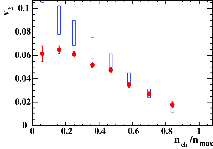
Figure 1: Elliptic flow (solid points) as a function of centrality defined as $n_{ch}/n_{max}$. The open rectangles show a range of values expected for $v_{2}$ in the hydrodynamic limit, scaled from $\epsilon$, the initial space eccentricity of the overlap region. From Ackermann:2000tr

Elliptic flow has its origin in the amount of rescattering and the spatial eccentricity of the collision zone. The amount of rescattering is expected to increase with increasing centrality, while the spatial eccentricity decreases. This combination of trends dominates the centrality dependence of elliptic flow. The spatial eccentricity is defined by

$$\epsilon=\frac{\langle y^{2}-x^{2}\rangle}{\langle y^{2}+x^{2}\rangle}$$

where $x$ and $y$ are the spatial coordinates in the plane perpendicular to the collision axis. The brackets $\langle\rangle$ denote an average weighted with the initial density.

Figure 1 shows the first measurement of elliptic flow at RHIC Ackermann:2000tr . Generally speaking, large values of elliptic flow are considered signs of hydrodynamic behavior as was first put forward by Ollitrault Ollitrault:1992bk . In hydrodynamics $v_{2}$ is essentially proportional to the spatial eccentricity (the strength depends on the velocity of sound of the matter). The open rectangles in Fig. 1 show, for a range of possible values of the velocity of sound, the expected $v_{2}$ values from ideal hydrodynamics. For  $n_{ch}/n_{max}\geq 0.5$ (${\bf b}\leq 7$ fm) it is observed that the data is well described by ideal hydrodynamics.

The observed large amount of collective flow, in particular elliptic flow, is one of the main experimental discoveries at RHIC Arsene:2004fa ; Back:2004je ; Adams:2005dq ; Adcox:2004mh and the main evidence suggesting nearly perfect fluid properties of the created matter RHIC_Discoveries .

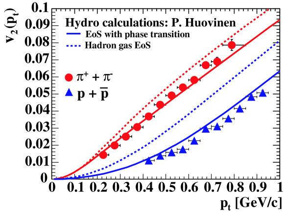
Figure 2: Elliptic flow of pions and protons as function of transverse momentum Adler:2001nb . The lines are hydrodynamical model calculations using two different Equations of State (EoS), the dashed lines represent calculations done with a hadron gas EoS while the solid curves are calculation with an EoS which incorporates the QCD phase transition.

Figure 2 shows $v_{2}$ for identified particles as function of transverse momentum. At low $p_{\mathrm{t}}$ the elliptic flow depends on the mass of the particle with $v_{2}$ at a fixed $p_{\mathrm{t}}$ decreasing with increasing mass. This dependence is expected in a scenario where all the particles have a common radial flow velocity Borghini:2001ys ; Blaizot:2001tf as shown by the curves in Fig. 2 from ideal hydrodynamics. The difference between the dashed and solid curves is the EoS, the dashed curves correspond to calculations done with a hadron resonance gas EoS while the solid curves are hydro calculations incorporating the QCD phase transition. The sensitivity to the EoS is better for the heavier particles because they are less affected by the contribution of the finite freeze-out temperature. It is clear that the hydro calculations incorporating the QCD phase transition give better description of the observed mass splitting. However, detailed constrains on the EoS can only be obtained with better modeling of the hadronic phase Teaney:2001av ; Teaney:2000cw ; Hirano:2005wx ; Hirano:2005xf and the transition Huovinen:2005gy between the QGP and hadronic phase.

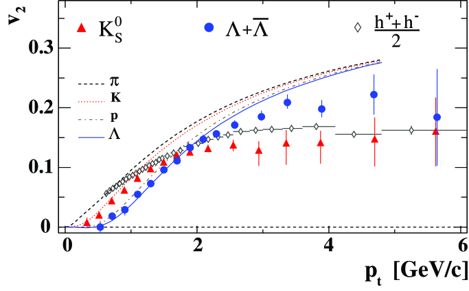
Figure 3: The minimum-bias (0–80% of the collision cross section) $v_{2}(p_{T})$ for $K_{S}^{0}$, $\Lambda+\overline{\Lambda}$ and $h^{\pm}$. Hydrodynamical calculations of $v_{2}$ for pions, kaons, protons and lambdas are also plotted Huovinen:2001cy . From Adams:2003am

In ideal hydrodynamics the mass ordering in $v_{2}$ persists up to arbitrary large $p_{\mathrm{t}}$, although less pronounced because the $v_{2}$ of the different particles start to approach each other. Figure 3 shows that at higher $p_{\mathrm{t}}$ the measurements start to deviate significantly from hydrodynamics for all particle species, and that the observed $v_{2}$ of the heavier baryons is larger than that of the lighter mesons. This mass dependence is the reverse of the behavior observed at low $p_{\mathrm{t}}$. This is not expected in hydrodynamics and is also not expected if the $v_{2}$ is caused by parton energy loss (in the latter case there would, to first order, be no particle type dependence). An elegant explanation of the unexpected particle type dependence and magnitude of $v_{2}$ at large $p_{\mathrm{t}}$ is provided by the coalescence picture Voloshin:2002wa ; Molnar:2003ff .

With the models which successfully describe the properties of the matter created at RHIC one can (and should) make predictions for the LHC. Testing these predictions will provide important confirmation of, or perhaps new insights to, our current understanding of QCD matter. Figure 4 shows elliptic flow calculations for the LHC.

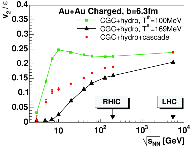
Figure 4: Theoretical predictions Hirano:2005 of $v_{2}/\epsilon$ versus collision energy using color glass condensate estimates for the initial conditions. Ideal hydrodynamic expansion up to kinetic freeze-out (squares) or chemical freeze-out (triangles) is assumed. The full circles are results using a hadronic cascade model to describe the final phase after chemical freeze-out.

Using Color Glass Condensate (CGC) estimates for the initial condition the flow is calculated using ideal hydrodynamics up to the kinematic freeze-out temperature of 100 MeV (full squares and upper curve). More realistic estimates are obtained by assuming hydrodynamics up to the chemical freeze-out temperature of 169 MeV followed by a hadron cascade description of the final phase (full circles). The contribution from the QGP phase (i.e. hydrodynamics up to 169 MeV) is shown by the triangles (and lower curve) in the figure. It is seen from Fig. 4 that at LHC energies the contribution from the QGP phase is much larger than at RHIC or SPS, and that, as a consequence, there is less uncertainty due to the detailed modeling of the hadronic phase. Theoretical calculations such as these or e.g. in Ref. Kolb:2000sd , as well as straight-forward extrapolations from lower energies based on particle multiplicities predict maximum flow values of about 5–10% at the LHC. If the flow values (and corresponding multiplicities) at the LHC are indeed that large then the flow measurement should be relatively easy.

However, the previous hydro estimates assume that during the QGP phase the matter has zero shear viscosity. Teaney Teaney:2003kp has shown that even a small shear viscosity has a large effect on the buildup of flow. Recent calculations Hirano:2005wx ; Csernai:2006zz show how the viscosity increases from RHIC to the LHC. To estimate how this would affect the predicted flow, viscous corrections have to be implemented in hydro models Heinz:2005zi .

In addition, experimental measurements of flow are affected by biases from physical effects unrelated to anisotropic flow (‘non-flow effects’ like e.g. jet correlations) or due to additional features of the flow signal itself (e.g. fluctuations Miller:2003kd ; Voloshin:2006gz ; Bhalerao:2006tp ; Alver:2006pn ). To estimate the effect of jet like correlations at the LHC a simple estimate can be made similar to what was done for the first RHIC flow measurement Ackermann:2000tr . The estimate of the non-flow is given by

$$\langle\cos[n(\Psi_{2}^{a}-\Psi_{2}^{b})]\rangle\propto M_{sub}v_{2}^{2}+\tilde{g},$$ (1)

where the angular brackets denote an average over the events, $\Psi_{2}^{a,b}$ are the subevent event planes, $M_{sub}$ is the corresponding subevent multiplicity and $\tilde{g}$ is the non-flow component. The estimated value of $\tilde{g}$ from HIJING at $\sqrt{s_{NN}}=$ 130 GeV in the STAR acceptance using random subevents was 0.05. In the ALICE TPC acceptance the value of $\tilde{g}$ from HIJING at $\sqrt{s_{NN}}=$ 5.5 TeV is found to be 0.08. With better tuned definitions of the subevents the value of $\tilde{g}$ could easily be reduced to 0.04. The correlation due to flow, $M_{sub}v_{2}^{2}$, is expected to be much larger than the non-flow contribution, 0.04, in a large centrality range for Pb+Pb collisions measured by ALICE at the LHC. This then indeed suggest that measuring flow can be done in great detail at the LHC.

3 Higher Harmonics

Higher harmonics of the momentum anisotropy are generally expected to be small Kolb:1999it ; Teaney:1999gr . More recently it was realized that at higher $p_{\mathrm{t}}$ they may become significant, in addition, that they are sensitive to the initial conditions Kolb:2003zi and that they depend on the equation of state Huovinen:2005gy . In Ref. Borghini:2005kd ; Bhalerao:2005mm it is argued that in particular $v_{4}$ in combination with $v_{2}$ probes ideal fluid behavior, because for an ideal fluid the ratio $v_{4}(p_{\mathrm{t}})/v_{2}^{2}(p_{\mathrm{t}})$ should approach 0.5.

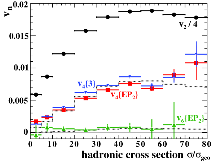
Figure 5: The $p_{t}$- and $\eta$- integrated values of $v_{2}$, $v_{4}$, and $v_{6}$ as a function of centrality. The dotted histograms are $1.4\cdot v_{2}^{2}$ and $1.4\cdot v_{2}^{3}$. In $v_{n}\{\}$ the term in the curly brackets indicates the method used Borghini:2001vi . Figure from Adams:2003zg .

The measured $p_{\mathrm{t}}$-integrated $v_{4}$ and $v_{6}$ as function of centrality are shown in Fig. 5 Adams:2003zg . For comparison, $v_{2}$ is shown in the same figure. The integrated $v_{4}$ is an order of magnitude smaller than $v_{2}$, as expected. The higher harmonics $v_{6}$ and $v_{8}$ (not shown) are consistent with zero. Figure 5 shows that the ratio $v_{4}/v_{2}^{2}$ is larger than unity for all centralities which seems in contradiction with the prediction for ideal fluid behavior. However Ref. Borghini:2005kd ; Bhalerao:2005mm shows that this asymptotic value of $v_{4}=v_{2}^{2}/2$ is reached at transverse momenta well above 1 GeV/c. At these higher transverse momenta hydrodynamics is expected to break down and thus the ratio $v_{4}/v_{2}^{2}$ expected to increase again. In addition, at RHIC the integrated ratio of $v_{4}/v_{2}^{2}$ is mainly determined by particles below 1 GeV/$c$, and is therefore not so well suited for this comparison.

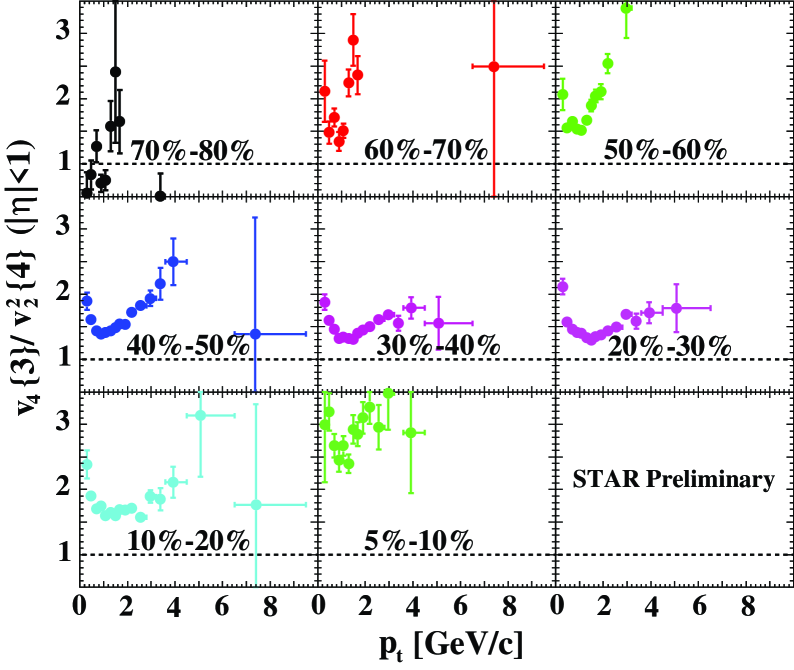
Figure 6: Centrality dependence of $v_{4}\{3\}/v_{2}^{2}\{4\}$ in Au+Au collisions at $\sqrt{s_{NN}}=$ 200 GeV. From TANG:2006xx

A better comparison is the transverse momentum dependence of $v_{4}/v_{2}^{2}$ shown in Fig. 6 for eight centralities. Below $p_{\mathrm{t}}$= 1.5 GeV/c the transverse momentum dependence is in agreement with hydro expectation. However for each of the centralities the minimum of $v_{4}/v_{2}^{2}$ is still more than a factor of two larger than the asymptotic ideal hydro value. Measurements of the energy dependence of this ratio, particularly at an order of magnitude higher beam energy at the LHC, should provide insight into the dynamics driving this ratio Bhalerao:2005mm .

4 Conclusions

At RHIC the observed large elliptic flow provides compelling evidence for strongly interacting matter which, in addition, appears to behave like an almost ideal fluid RHIC_Discoveries . At low $p_{\mathrm{t}}$ the ratio $v_{4}/v_{2}^{2}$, exhibits the transverse momentum dependence expected for an ideal fluid while, as expected, deviating at higher $p_{\mathrm{t}}$. However, the magnitude of $v_{4}/v_{2}^{2}$ is still more than a factor of two larger than the asymptotic ideal hydro value. At the LHC the expected increase in multiplicity together with the expected increase in anisotropic flow will allow for a detailed measurement of the $v_{2}$ and higher harmonics ALICEppr . These measurements are expected to quickly provide important confirmations, or perhaps new insights to our current understanding of the EoS of QCD matter.

References

- (1) J. Y. Ollitrault, Phys. Rev. D 46 (1992) 229.
- (2) P. Danielewicz, Nucl. Phys. A 661 (1999) 82.
- (3) D. H. Rischke, Nucl. Phys. A 610 (1996) 88C.
- (4) J. Y. Ollitrault, Nucl. Phys. A 638 (1998) 195.
- (5) S. Voloshin and Y. Zhang, Z. Phys. C 70 (1996) 665.
- (6) K. H. Ackermann et al. [STAR Collaboration], Phys. Rev. Lett. 86 (2001) 402
- (7) I. Arsene et al. [BRAHMS Collaboration], Nucl. Phys. A 757 (2005) 1
- (8) B. B. Back et al. [PHOBOS Collaboration], Nucl. Phys. A 757 (2005) 28
- (9) J. Adams et al. [STAR Collaboration], Nucl. Phys. A 757 (2005) 102
- (10) K. Adcox et al. [PHENIX Collaboration], Nucl. Phys. A 757 (2005) 184
- (11) T.D. Lee et al., New Discoveries at RHIC: Case for the Strongly Interacting Quark-Gluon Plasma. Contributions from the RBRC Workshop held May 14-15, 2004. Nucl. Phys. A 750 (2005) 1-171
- (12) C. Adler et al. [STAR Collaboration], Phys. Rev. Lett. 87 (2001) 182301
- (13) N. Borghini, P. M. Dinh and J. Y. Ollitrault, arXiv:hep-ph/0111402.
- (14) J. P. Blaizot, Nucl. Phys. A 698 (2002) 360.
- (15) D. Teaney, J. Lauret and E. V. Shuryak, arXiv:nucl-th/0110037.
- (16) D. Teaney, J. Lauret and E. V. Shuryak, Phys. Rev. Lett. 86 (2001) 4783.
- (17) T. Hirano and M. Gyulassy, Nucl. Phys. A 769 (2006) 71
- (18) T. Hirano, U. W. Heinz, D. Kharzeev, R. Lacey and Y. Nara, arXiv:nucl-th/0511046.
- (19) P. Huovinen, Nucl. Phys. A 761 (2005) 296
- (20) P. Huovinen, P. F. Kolb, U. W. Heinz, P. V. Ruuskanen and S. A. Voloshin, Phys. Lett. B 503 (2001) 58
- (21) J. Adams et al. [STAR Collaboration], Phys. Rev. Lett. 92 (2004) 052302
- (22) S. A. Voloshin, Nucl. Phys. A 715 (2003) 379.
- (23) D. Molnar and S. A. Voloshin, Phys. Rev. Lett. 91, 092301 (2003)
- (24) T. Hirano, Talk given at the Workshop on QGP Thermalization (QGPTH05), Vienna, Private communication.
- (25) P. F. Kolb, J. Sollfrank and U. W. Heinz, Phys. Rev. C 62 (2000) 054909.
- (26) D. Teaney, Phys. Rev. C 68 (2003) 034913
- (27) L. P. Csernai, J. I. Kapusta and L. D. McLerran, arXiv:nucl-th/0604032.
- (28) U. W. Heinz, arXiv:nucl-th/0512049.
- (29) M. Miller and R. Snellings, arXiv:nucl-ex/0312008.
- (30) S. A. Voloshin, arXiv:nucl-th/0606022.
- (31) R. S. Bhalerao and J. Y. Ollitrault, arXiv:nucl-th/0607009.
- (32) B. Alver [the PHOBOS Collaboration], arXiv:nucl-ex/0608025.
- (33) P. F. Kolb, J. Sollfrank and U. W. Heinz, Phys. Lett. B 459 (1999) 667.
- (34) D. Teaney and E. V. Shuryak, Phys. Rev. Lett. 83 (1999) 4951.
- (35) P. F. Kolb, Phys. Rev. C 68 (2003) 031902.
- (36) N. Borghini and J. Y. Ollitrault, arXiv:nucl-th/0506045.
- (37) R. S. Bhalerao et al., Phys. Lett. B 627 (2005) 49.
- (38) N. Borghini, P. M. Dinh and J. Y. Ollitrault, Phys. Rev. C 64 (2001) 054901
- (39) J. Adams et al. [STAR Collaboration], Phys. Rev. Lett. 92 (2004) 062301
-
(40)
A.H. Tang [for the STAR Collaboration],
arXiv:nucl-ex/0608026
Y. Bai, 2006 RHIC & AGS Annual Users’ Meeting, http://www.bnl.gov/rhic_ags/users_meeting/Workshops/8.asp - (41) The ALICE collaboration, PPR Vol I: J. Phys. G 30 (2004) 1517, PPR Vol II: CERN/LHCC 2005-030