Comparisons of Statistical Multifragmentation and Evaporation Models for Heavy Ion Collisions

Abstract

The results from ten statistical multifragmentation models have been compared with each other using selected experimental observables. Even though details in any single observable may differ, the general trends among models are similar. Thus these models and similar ones are very good in providing important physics insights especially for general properties of the primary fragments and the multifragmentation process. Mean values and ratios of observables are also less sensitive to individual differences in the models. In addition to multifragmentation models, we have compared results from five commonly used evaporation codes. The fluctuations in isotope yield ratios are found to be a good indicator to evaluate the sequential decay implementation in the code. The systems and the observables studied here can be used as benchmarks for the development of statistical multifragmentation models and evaporation codes.

I Introduction

During the later stages of a central collision between heavy nuclei at incident energies in excess of about $E/A$=50 MeV, a rapid collective expansion of the combined system occurs ref1 . Experimental evidence indicates that mixtures of intermediate mass fragments (IMF’s) with $3\leq Z\leq 30$ and light charged particles (LCP, $Z\leq 2$) are emitted during this expansion stage. With increased nucleon collisions, the properties of the nuclear matter created can be described with equilibrium and statistical concepts ref2 ; ref3 ; ref4 ; ref5 ; ref6 ; ref6b ; ref6c ; ref7 ; ref8 ; ref9 . Ultimately, one would like to describe nuclear collisions with a model that takes into account all the dynamics of nucleon-nucleon collisions. Until then, statistical models provide invaluable insight to the physics of multifragmentation of the last three decades, by reducing the intractable problem of time-dependent highly correlated interacting many-body fermion system to the much simpler picture of a system of non-interacting clusters ref10 .

Since most statistical multifragmentation codes have been developed to describe specific sets of data and nearly all of them have different assumptions, they are not equivalent ref2 ; ref3 ; ref4 ; ref5 ; ref6 ; ref6b ; ref6c ; ref7 ; ref8 ; ref9 ; ref11 ; ref11b ; ref12 ; ref13 ; ref14 ; ref15 . One of the goals of this article is to examine the observables constructed with the isotope yields from different statistical multifragmentation models used in recent years. Even though the number of models we studied is limited, they represent the codes widely used in the heavy ion community. The results show that all the statistical codes give similar general trends but different predictions to specific experimental observables. The conclusion is consistent with a recent study on models with different statistical assumptions ref17 . We also find that the differences between models are much reduced for observables constructed with isotope yield ratios from different reactions.

The various codes and the bench mark systems which form the basis for comparison will be described in Section 2. Comparisons of the statistical multifragmentation models are presented in Section 3 and the results from the comparisons of five different evaporation codes are presented in Section 4. Finally we summarize our findings in Section 5.

Table 1: Summary of the different statistical multifragmentation models and evaporation codes studied in this article.

Code	Evaporation	user	author	Ref.	(168,75)	(186,75)	(168,50)	Primary	Final
Statistical Multifragmentation Models
ISMM-c	MSU-decay	Tsang	Das Gupta	2	Y	Y		Y	Y
ISMM-m	MSU-decay	Souza	Souza	13,14	Y	Y		Y	Y
SMM95	own code	Bougault	Botvina	4, 9	Y	Y		Y	Y
MMM1	own code	AH Raduta	AH Raduta	15	Y	Y	Y	Y	Y
MMM2	own code	AR Raduta	AR Raduta	15	Y	Y	Y	Y	Y
MMMC	own code	Le Fèvre	Gross	5, 16	Y	Y	Y		Y
LGM	N/A	Regnard	Gulminelli	17	Y		Y	Y
QSM	own code	Trautmann	Stöcker	18	Y	Y	Y		Y
EES	EES	Friedman	Friedman	7, 8	Y	Y	Y	Y	Y
BNV-box	N/A	Colonna	Colonna	24	Y	Y		Y
Evaporation codes
Gemini		Charity	Charity	25	Y	Y			Y
Gemini-w		Wada	Wada	25–28	Y	Y			Y
SIMON		Durand	Durand	29	Y	Y			Y
EES		Friedman	Friedman	7, 8	Y	Y	Y		Y
MSU-decay		Tsang	Tan et al.	14	Y	Y			Y

II Bench-mark systems

Nearly all statistical models assume that nucleons and fragments originate from a single emission source characterized by $A_{0}$ nucleons and $Z_{0}$ protons. The hot fragments then de-excite using evaporation models. To provide consistent comparisons between models, we have chosen the following source systems: 1) $A_{0}$=168, $Z_{0}$=75, $N_{0}$/$Z_{0}$=1.24, 2) $A_{0}$=186, $Z_{0}$=75, $N_{0}$/$Z_{0}$=1.48. These two systems have the same charge and are chosen to be 75% of the initial compound systems of ¹¹²Sn+¹¹²Sn and ¹²⁴Sn+¹²⁴Sn ref18 ; ref19 . We also have calculations on system 3) $A_{0}$=168, $Z_{0}$=84, $N_{0}$/$Z_{0}$=1.0 which has the same mass but different charge from system 1. Even though most results of system 3 are not included in this article due to lack of space, they corroborate the conclusions. In each calculation, the same inputs are used. We require the source excitation energy, $E^{\star}$, to be 5 MeV per nucleon and the source density to be 1/6 of the normal nuclear matter density.

At the time when this manuscript was prepared, we were able to get results from nine statistical multifragmentation model codes plus a hybrid dynamical-statistical code, (BNV-box) and five evaporation codes. Table 1 lists all the codes, users (defined as the person who did the calculations shown in this paper) and the main authors of the codes. The users sent us the output files which contain mainly the neutron ($N$) and proton ($Z$) number and the yield of the hot fragments and/or the final fragments. All these output files can be found in the web: http://groups.nscl.msu.edu/smodels/results.html.

The statistical multifragmentation models studied here construct fragment yields from a maximum entropy principle, but they differ both in the degrees of freedom employed and in the chosen constraints. We have different versions of the Statistical Multifragmentation Model (SMM) ref20 . All these models assume that the N-body source correlations are exhausted by clusterization and, therefore, describe the system as a collection of non-inter-acting clusters. (The Coulomb repulsion among fragments are approximately taken into account.) These codes differ in the freeze out volume prescription, in the treatment of continuum states and in the numerical technique to span the phase space. The SMM95 code uses grand-canonical approximation ref4 ; ref7 and Fermi-jet breakups for the deexcitation of hot fragments. The Improved Statistical Multifragmentation Model (ISMM) ref11b uses experimental masses and level densities when available. When experimental information is not available, ISMM uses an improved algorithm to interpolate level densities for the hot fragments. It uses the MSU-decay code as an afterburner. ISMM-c ref2 uses a canonical formalism, while ISMM-m ref11 adopts a microcanonical approach. The sequential decay algorithm in ISMM ref11 uses experimental masses and includes structure information for light fragments $(Z<15)$. The MMMC code uses a Metropolis-Monte Carlo method ref5 ; ref13 . MMMC is the only model that can accommodate non-spherical sources but only neutrons are emitted in the sequential decays. We have two calculations using the microcanonical multifragmentation model MMM ref12 with different freeze-out assumptions: (1) non-overlapping spherical fragments inside a spherical source and (2) free volume approach. These two calculations are correspondingly denoted by MMM1 and MMM2. The Quantum Statistical Model (QSM) ref15 is a simplified grand-canonical version of SMM models including only a limited number of light clusters $(A<20)$, which however are described with a detailed density of states accounting for all known discrete levels at the time when the code was written in the late eighties.

The Expanding Emitting Source (EES) model ref6b ; ref6c is an extended Weisskopf evaporation model ref15b which couples the emission of fragments to the changing conditions, i.e., density (volume), mass-number, isospin, and entropy, of the source. The model assumes an equation-of-state for the source so that the thermal pressure and initial expansion determine the changes in the source due to emission. It is the only statistical model to account for the time dependence of the emission process. No specific density (volume) for emission is assumed, but the model predicts that the strongest emission often occurs from a dilute source during a narrow time period. (In this sense it is similar to the SMM.) Spectra are constructed by summing the contributions of emission from different times, with a switch from surface to volume emission at a low density of the source.

Finally, we have two microscopic model calculations. The Lattice Gas Model (LGM) ref14 calculates the equilibrium configurations of a system of (semi)classical nucleons interacting via an Ising Hamiltonian. These configurations are generated in a given confining box by Monte Carlo. It is the only model that has no nuclear physics input. The BNV-box model is based on the Boltzmann-Nordheim Vlaslov (BNV) equations ref16 and uses the effective Skyrme force augmented with a stochastic collision integral to calculate the equilibrium configurations which are generated via a dissipation dynamics in a box. In both models, the clusters have to be defined a posteriori via a clusterization algorithm.

Since de-excitation of the hot fragments is essential before comparison to experimental data, most codes have their own sequential decay algorithms. Ideally, one should compare the hot primary fragments and the decay fragments separately. Unfortunately, in some codes (e.g. MMMC), the hot fragments cannot be extracted while in others (LGM and BNV-box) the hot fragments sent by the users have not undergone decay. This makes comparing the contributions from the evaporation portion of the code to the final fragments very difficult.

Since an ”after-burner” or evaporation code is needed to allow the hot fragments to decay to ground states, codes that can be coupled to statistical and dynamical codes are very important. Thus in addition to the fragmentation models, we also compare five different evaporation codes (listed in Table 1) that have served the functions of ”after-burners” to both statistical and dynamical codes. 1.) The most widely used code is Gemini ref21 which treats the physics of excited heavy residues very well. However, for the light fragments, it lacks complete structural information. 2.) A modified code of an early version of Gemini ref22 ; ref23 has also been used extensively to de-excite hot fragments generated in the Asymmetrized Molecular Dynamical (AMD) Model ref24 . We labeled this modified version of Gemini as Gemini-w. 3.) An event generator code called SIMON ref25 , based on Weisskopf emission rates ref15b , includes the narrowest discrete states for $Z\leq 9$ as well as in-flight evaporation. It has been used to deexcite fragments created in both BNV dynamical model ref26 and a heavy-ion phase space model ref27 . 4.) The MSU-decay code ref11b uses the Gemini code to decay heavy residues and includes much structural information such as the experimental masses, excited states with measured spin and parity for light fragments with $Z<15$ in a table. This table also includes information of calculated states, which are not measured. 5.) In principle, at very low excitation energy, the multifragmentation models can also be used as evaporation models. In this category, we have results from the EES model ref6b ; ref6c .

For the evaporation model comparison, the bench mark systems for the source are the same as the three systems used in the multifragmentation models, $(A_{0},Z_{0})=(168,75),(186,75)$ and $(168,84)$. The excitation energy is set to be 2 MeV per nucleon and the density is assumed to be the same as normal nuclear matter density.

III Results from multifragmentation models

In this section, we choose to show results that illustrate the differences and similarities between calculations. Due to limited space, not all observables from the calculations are constructed or shown here. Since system 1 with $A_{0}$=168 and $Z_{0}$=75 have results from all the calculations, we tend to highlight this system. Some of the results on the ISMM-c calculations have been published in ref. ref2 . If a choice has to be made between showing ISMM-c results or ISMM-m results due to lack of space, we choose to show the results of ISMM-m. For the LGM calculations ref14 ; ref28 , we have results using the micro-canonical approximations as well as results using canonical approximations. We show mainly the results with the microcanonical approximations. The differences between the microcanonical and canonical assumptions can be inferred from the results of ISMM-c and ISMM-m. The observables shown in Sections 3.1 to 3.5 are chosen for the relevance of the observables to the understanding of the multifragmentation process. More recently, the focus of heavy ion collisions at intermediate energy has shifted to explore the isospin degree of freedom ref2 . This is often done by studying two or more systems, which differ mainly in the isospin composition of the projectiles or targets. Isoscaling using isotope yield ratios is discussed in Section 3.4. Instead of using isotope yield ratios for temperature, we use the fluctuations of different thermometers to determine how well the sequential decays in the code reproduce the observed fluctuations. The results will be described in Section 3.5.

To provide some uniformity to the figures, we will try to use the same symbols for the results from the same code throughout this article. Where applicable, closed symbols often refer to the neutron rich system ($A_{0}$=186, $Z_{0}$=75) and open symbols refer to the neutron deficient system ($A_{0}$=168, $Z_{0}$=75). We also adopt the convention that the results are labeled with the user (who sent us the calculated results) and the code name. Even though comparison with data is not our goal, it is sometimes instructive to plot the data as reference points when appropriate. We have chosen the data from the central collisions of ¹²⁴Sn+¹²⁴Sn and ¹¹²Sn+¹¹²Sn ref18 ; ref19 at 50 MeV per nucleon incident energy as represented by closed and open star symbols, respectively, mainly because this data set is readily available to the first author.

III.1 IMF multiplicities

The copious production of intermediate mass fragments (IMF) which are charged particles with $Z$=3-20 is one signature of the multifragmentation process. The study of these fragments provides clues to the nuclear liquid-gas phase transition as they are considered as droplets formed from the condensation of nuclear gas and may provide information about the co-existence region. Figure 1 shows the mean multiplicities of IMFs produced by different models. Within errors, one cannot discern any dependence of the mean IMF multiplicity on the isospin composition of the initial sources by looking for systematic differences between solid and open symbols which represent the neutron-rich and neutron-deficient systems, respectively. If we compare the left and right panel of Fig. 1, in general, sequential decays reduce the IMF multiplicities.

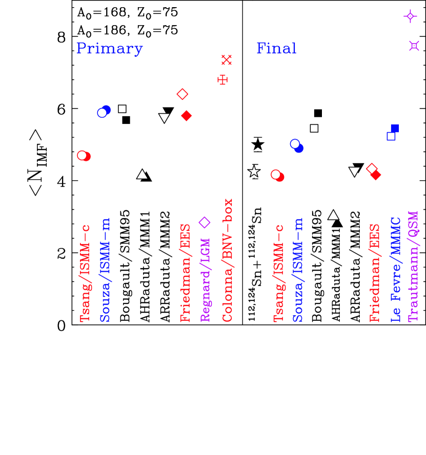
Figure 1: Mean IMF multiplicity obtained from different statistical models listed in Table 1 for primary fragments (left panel) and final fragments (right panel). At the bottom of the panels, the calculations are labeled by the name of the user and the name of the code. The open symbols refer to system 1 ($A_{0}$=168, $Z_{0}$=75) and the solid symbols refer to system 2 ($A_{0}$=182, $Z_{0}$=75). The open and solid stars in the right panel are data from the central collisions of ¹¹²Sn+¹¹²Sn and ¹²⁴Sn+¹²⁴Sn systems at $E/A$=50 MeV ref32 .

The two MMM calculations have different results due to different freeze out assumptions used for the source. MMM1 which uses non-overlapping spherical fragments emits nearly two fragments less than MMM2. Only primary fragments before decay are available from the LGM and BNV-box calculations. For the MMMC and QSM models, we only have fragments after decay.

For the primary fragment multiplicity (left panel), the BNV model emits slightly more primary fragments while the LGM model emits nearly a factor of two less fragments than the other models. For the final fragment multiplicity (right panel), the QSM ref15 ; ref29 ; ref30 emits many more IMFs. Indeed this model is not suited to predict absolute yields but rather should be used to compute relative yields of light isotopes e.g. for thermometry purposes ref30 ; ref31 . For comparisons, the data from the central collisions of Sn isotopes are represented by the star symbols in the right panel. The differences in the mean multiplicities between the ¹¹²Sn+¹¹²Sn (open stars) and ¹²⁴Sn+¹²⁴Sn (solid stars) ref32 are much larger than those predicted by all the models after decay. The discrepancies between model predictions and data are not understood.

III.2 Mass Distributions

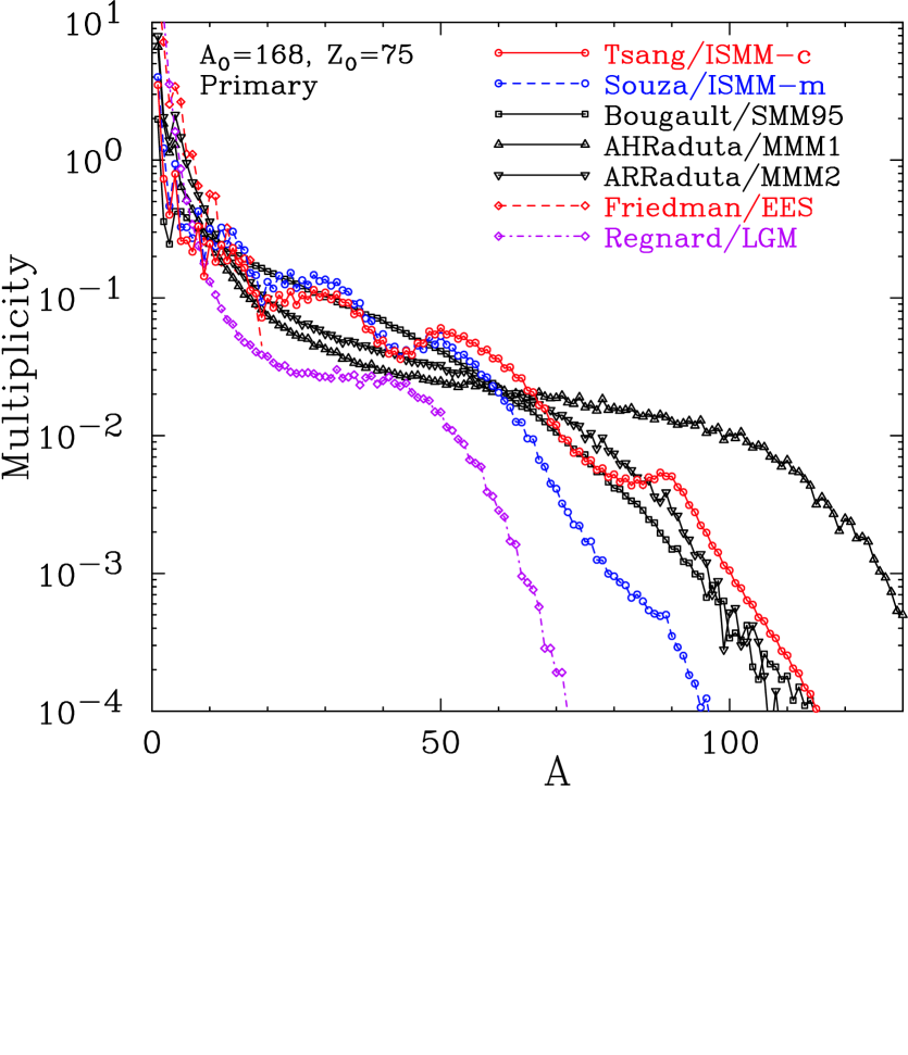
Figure 2: Predicted primary fragment mass distributions from the mutifragmentation of a source nucleus with $A_{0}$=168, $Z_{0}$=75 (system 1). See caption of Fig. 1 for name convention.

Next we examine the primary mass distributions of the $A_{0}$=168, $Z_{0}$=75 system. The steep drop of the light fragment ($A<10$) multiplicity shown in Fig. 2 are similar for nearly all the models but there are differences. Some of the differences (e.g. between MMM1 (upright triangles) and MMM2 (inverted triangles) arise from differences in the freeze-out assumptions as described previously. The differences in the results from the two ISMM calculations may come from the difference between canonical and micro-canonical approximations used. (ISMM-c requires temperature instead of excitation energy as one property of the initial source.) SMM95 and the two MMM calculations have smooth distributions as the fragment masses are determined from liquid drop mass-formulae ref33 . The LGM (the lowest curve with diamond symbols), which does not take into account the binding energies or nucleon masses shows a smooth dependence on mass but does not produce heavy residues.

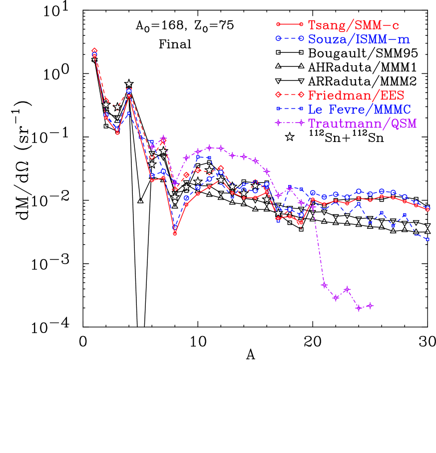
Figure 3: Predicted final fragment mass distributions from the multifragmentation of a source nucleus with $A_{0}$=168, $Z_{0}$=50 (system 1). For comparison, data from the multifragmentation of central collisions of ¹¹²Sn+¹¹²Sn system ref2 ; ref18 at $E/A$=50 MeV are plotted as open stars.

In Figure 3, we have plotted the differential multiplicity of the final mass distributions for the same ($A_{0}$=168, $Z_{0}$=75) system in an expanded scale. Again, while the trends are similar for most calculations except the QSM model (crosses), there are significant differences in detailed comparisons. Most models do not have nuclei with mass 5 and cross-sections for mass 8 are much reduced in accordance to experimental observation. For reference, the data from the ¹¹²Sn+¹¹²Sn system are plotted as open stars. The trends exhibited by most models are similar to those of the data. Primary and final fragments with $A\geq 20$ are ignored in the EES code. These heavy fragments are not included in the output files. The QSM does not produce fragments with $A>20$. To conserve the total number of nucleons, more light charged fragments with $A\leq 20$ are produced, causing the over-production of IMFs seen in both Figs. 1 and 3.

The charge distributions are similar to the mass distributions so they are not discussed here.

III.3 Isospin observables and isotope distributions

One observable to study the isospin degrees of freedom is the asymmetry, $N/Z$, of the fragments. Figure 4 shows $<N/Z>$ as a function of the fragment charge number $Z$ predicted by different models. In this plot, the left panel shows results from the neutron-deficient system ($A_{0}$=168, $Z_{0}$=75) while the right panel contains results from the neutron-rich system ($A_{0}$=186, $Z_{0}$=75). Unlike the mass distributions shown in Figs. 2 and 3, differences between different models are not very large, about 10%. (The zero of the vertical axis is suppressed in order to show the differences in more details.) As expected, the $<N/Z>$ of the fragments are larger for the more neutron rich system. However, the $<N/Z>$ values are much lower than the $<N_{0}/Z_{0}>$ of the initial system of 1.48 for the neutron-rich system. For the neutron-deficient system in the left panel, the initial $<N_{0}/Z_{0}>$ value is 1.24 which is only slightly larger than the fragment values. For reference, data from the central collisions of ¹²⁴Sn+¹²⁴Sn (solid stars) and ¹¹²Sn+¹¹²Sn systems (open stars) ref18 are plotted in the left and right panels, respectively. Since the excited fragments in MMMC only emit neutrons ref13 , the fragment $<N/Z>$ (squares) are lower than those derived from other models. All the other calculations exhibit similar trends as the data.

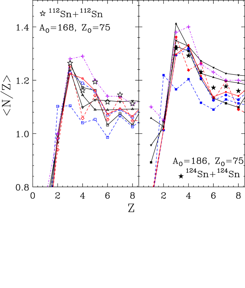
Figure 4: The mean neutron to proton ratios as a function of the charge of the emitted fragment $Z$ for system 1 (left panel) and system 2 (right panel). For comparison, results from the multifragmentation following central collisions of ¹¹²Sn+¹¹²Sn and ¹²⁴Sn+¹²⁴Sn are shown as open (left panel) and closed stars (right panel), data from ref. ref18 .

As the average values of the asymmetry of the fragments are determined from the isotope yields, it is instructive to examine the isotope distributions directly. Figure 5 shows the oxygen isotope distributions from different models before (left panels) and after (right panels) sequential decays. The upper panels indicate the isotopes from the neutron-rich ($A_{0}$=186, $Z_{0}$=75) system while fragments from the neutron-deficient ($A_{0}$=168, $Z_{0}$=75) system are plotted in the bottom panels. For reference, data ref18 from the central collisions of ¹²⁴Sn+¹²⁴Sn (solid stars) and ¹¹²Sn+¹¹²Sn systems (open stars) are plotted in the upper right panel and lower right panels, respectively.

The differences in the primary distributions between models (left panel) can be understood from the nuclear masses used in the different codes. Both the ISMM models (circle symbols) used experimental masses even for hot fragments ref2 ; ref11b , thus odd-even effects are evident in the primary mass distributions. The SMM95 (squares) ref7 and the two MMM (upright and inverted triangles) ref12 ; ref33 calculations use mass formulae resulting in smooth interpolations of isotope cross-sections. The deficiency of models like the LGM (open diamond symbols in the lower left panel), which do not include any nuclear physics information, is obvious. The EES results are not presented here as the model ignores primary and secondary fragments with $A/geq$20 and the oxygen isotope yields are not complete.

The isotope distributions from all models after decay (right panels) become much narrower and resemble that of the experimental data. The ISMM-c, ISMM-m and SMM95 models predict a peak at ¹⁶O due to its large binding energy and the use of experimental masses in the decays. The ISMM calculations that incorporate the MSU-decay algorithms with experimental masses and structural information exhibit odd-even effects. In the decay code of the MMM calculations, fragment masses are derived from mass formulae ref33 . As a result, the isotope distributions are rather smooth. The individual yields of oxygen isotopes are not available from the QSM output files, and the results of this model is not represented here.

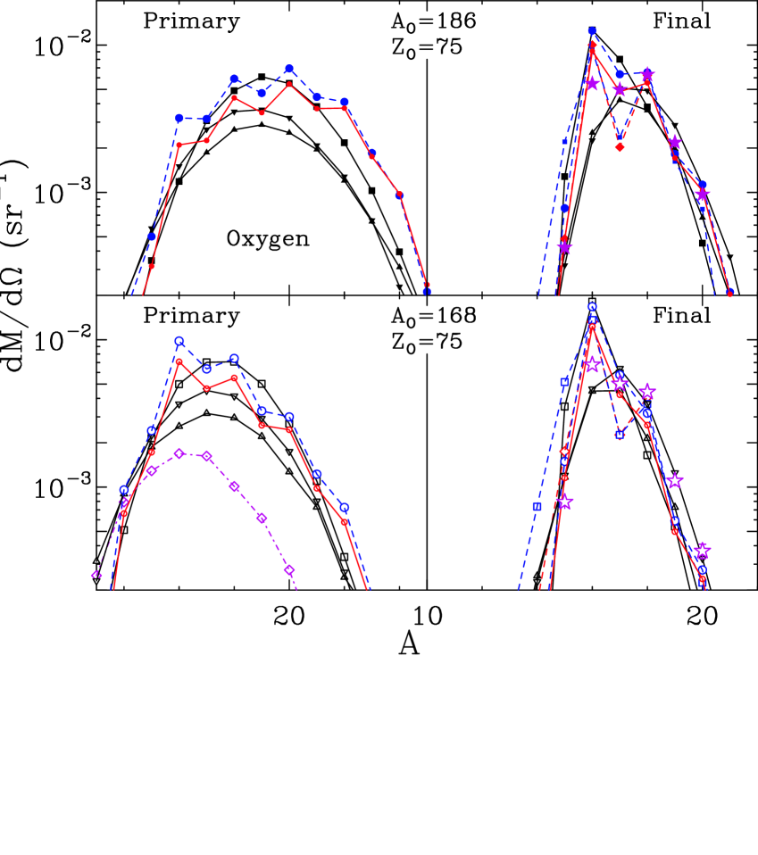
Figure 5: Predicted isotope distributions for oxygen fragments from different models. Primary fragments are plotted in the left panels and final fragments in the right panels. The top panels contain results from the neutron-rich system 2 and the bottom panels contain distributions from the neutron-deficient system 1. The open (bottom right panel) and solid stars (top right panel) are data from ref. ref18 .

In order to quantify the mean and the width of the distributions, we have plotted the mean mass number and the standard deviations of the oxygen distributions in Fig. 6 for both the primary (left panel) and final (right panel) fragment distributions. The vertical bars represent the standard deviations of the isotope distributions. In general, all models produce much wider distributions for the primary isotopes and the widths are reduced by sequential decay effects. Sequential decays tend to move the centroids of the distributions towards the valley of stability and reduce the differences in the centroids of the isotope distributions between the neutron-rich and neutron-deficient systems.

III.4 Isoscaling

When isoscaling was first observed in experimental data ref19 ; ref34 , it was demonstrated through statistical model calculations that isoscaling could be preserved through sequential decays ref34 ; ref35 . More importantly, statistical models relate the isoscaling phenomenon to the symmetry energy ref34 ; ref35 ; ref36 ; ref37 , which is of fundamental interest to general nuclear properties as well as astrophysical interests colonnabook .

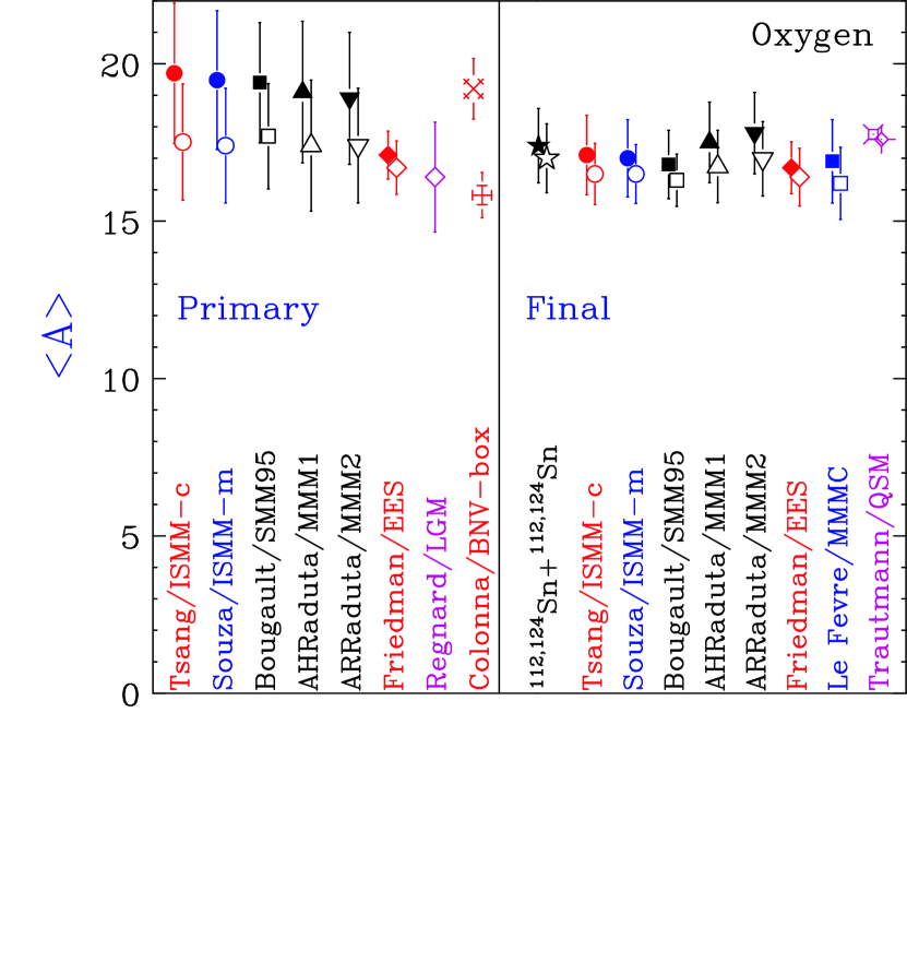
Figure 6: Centroids and widths (variance) of the oxygen isotope distributions obtained from different models. Most of the distributions are shown in Fig. 5.

Isoscaling describes the exponential dependence on the isotope neutron ($N$) and proton ($Z$) number of the yield ratios from two different reactions,

$$R_{21}=\frac{Y_{2}(N,Z)}{Y_{1}(N,Z)}=C\mathrm{e}^{\alpha N+\beta Z}$$ (1)

where $C$, $\alpha$, and $\beta$ are the fitting parameters. In our specific examples of systems 1 and 2, $Y_{2}(N,Z)$ is the isotope yield emitted from the neutron-rich system $A_{2}$=186, $Z_{2}$=75 and $Y_{1}(N,Z)$ is the isotope yield emitted from the neutron-deficient system $A_{1}$=168, $Z_{1}$=75. Figure 7 shows that all statistical multifragmentation models exhibit good isoscaling behavior for the primary fragments. Each symbol corresponds to one element, $Z$=1 (open triangles), $Z$=2 (closed triangles), $Z$=3 (open circles), $Z$=4 (closed circles), $Z$=5 (open squares), $Z$=6 (closed squares), $Z$=7 (open diamonds) and $Z$=8 (closed diamonds). The solid and dashed lines are best fits from Eq. (1). The slopes of the lines correspond to the neutron isoscaling parameter $\alpha$ and the distance between the lines corresponds to the isoscaling parameter $\beta$. All the models except LGM have similar slopes. The slope parameters from the two MMM models are slightly smaller. The LGM only has calculations on systems 1 and 3. Since the differences in the asymmetries between systems 1 and 2 and systems 1 and 3 are small, the LGM isoscaling slopes are expected to be slightly smaller but they are much smaller (lower left panel) than the other models. This is probably related to the lack of nuclear mass input in such model.

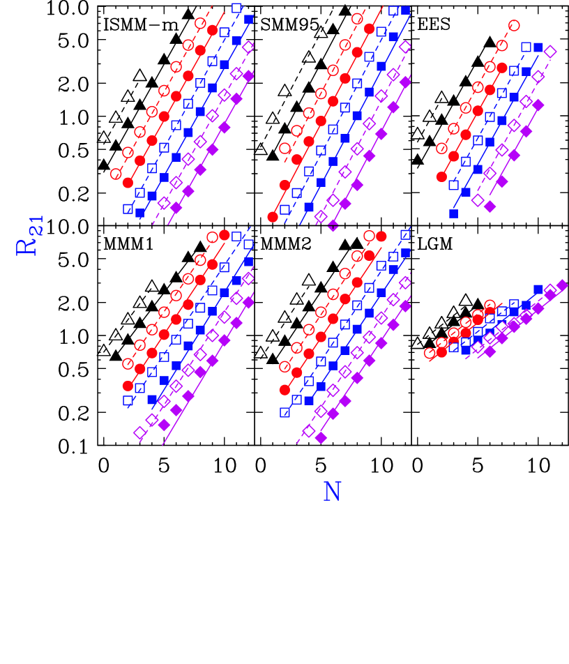
Figure 7: Predicted yield ratios, $R_{21}(N,Z)=Y_{2}(N,Z)/Y_{1}(N,Z)$ from primary fragments for system 2 and system 1. (For the LGM, the calculations are for system 1 and system 3.) Each panel presents the results from one model calculation. The lines are best fits to the symbols according to Eq. (1). Different lines correspond to atomic numbers $Z$=1 to 8 starting with the leftmost line being $Z$=1. Open points and dashed lines denote isotopes with odd $Z$ while solid points and solid lines denote isotopes with even $Z$.

An important contribution that statistical models make to the field of heavy ion collision is the derivation that the isocaling parameter $\alpha$ is related to the symmetry energy coefficient, $C_{sym}$.

$$\alpha_{pri}=\frac{4C_{sym}}{T}\left[\left(\frac{Z_{1}}{A_{1}}\right)^{2}-\left(\frac{Z_{2}}{A_{2}}\right)^{2}\right]=\frac{4C_{sym}}{T}\left[\left(\Delta\frac{Z}{A}\right)^{2}\right]$$ (2)

where $\alpha_{pri}$ is the isoscaling parameter extracted from the calculated yields of primary fragments, $T$ is the temperature, $Z_{i}/A_{i}$ is the proton fraction of the initial source with label i. To extract $C_{sym}$ which is related to symmetry energy ($E_{sym}=C_{sym}I^{2}$) from data, it is important that the sequential decays do not affect $\alpha$, $T$ and $[\Delta(Z/A)]^{2}$ significantly.

Figure 8 shows isoscaling plots constructed from final fragments after sequential decays. Isoscaling is no longer strictly observed over a large range of isotopes. Furthermore, the distances between elements are much less regular and the slopes vary from element to element. The distances between elements are related to the proton isoscaling parameter, $\beta$. Experimentally, the trends and magnitudes in both $\alpha$ and $\beta$ are similar ref19 ; geraci . The irregular spacings between elements from the calculations is probably caused by the Coulomb treatment in different codes. Part of the lack of smoothness in the trends could come from the lack of statistics for primary isotopes with low cross-sections. By restricting the isoscaling analysis to the same set of isotopes measured in experiments, about 3 isotopes for each element ref19 ; geraci , most models show that the effect from sequential decays on isoscaling is negligible as shown in the left panel of Fig. 9. The solid points refer to the analysis of the systems with the same charge, system 1 and 2 in Table 1, while the open points refer to the analysis of the systems with the same mass, system 1 and 3. In the two MMM calculations (triangles), the final fragments seem to retain more memory of the source than the other models as shown in Fig. 6, resulting in the final isoscaling parameters being larger than the primary isoscaling parameters. By restricting the number of isotopes for fitting, the problems with statistics from fragment production may be minimized. On the other hand, such procedure may hide fundamental problems associated with the sequential decays.

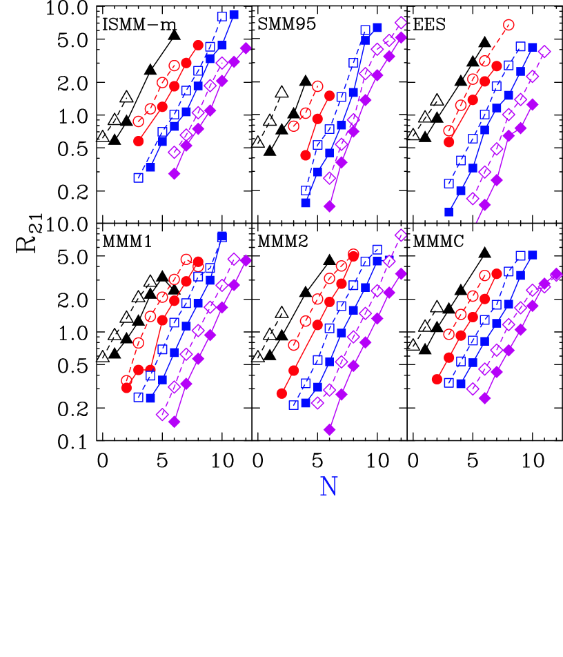
Figure 8: Predicted yield ratios, $R_{21}(N,Z)=Y_{2}(N,Z)/Y_{1}(N,Z)$ from final fragments. The symbols have the same convention as in Fig. 7. The lines are drawn to guide the eye.

All the statistical models except the LGM use the symmetry energy of stable nuclei in describing the mass of the fragments. Except for the EES model, the symmetry energy coefficient, $C_{sym}$, remains constant throughout the reactions. Such prescription may not be realistic. In a recent study, when different (especially lower) values of $C_{sym}$ are used in a Markov-chain version of the SMM95 code, the sequential decays effects are very different ref38 as shown in the right panel of Fig. 9. The lines denote different excitation energy (4, 6, 8 MeV) used. For each excitation energy, calculations have been performed for $C_{sym}=$ 4 (burst symbols), 8 (X symbols), 14 (crosses) and 25 (circular symbols) $MeV$. For $C_{sym}=25$ MeV, the effect of sequential decays are similar to those shown in the left panel of Fig. 9. However, for lower $C_{sym}$ values, the $\alpha$(final) are larger than $\alpha$(primary). As discussed in colonnabook , this trend is different from those observed in dynamical calculations. A detailed understanding of the effects of sequential decays on the isoscaling parameters $\alpha$, the temperature $T$, and the proton fraction $Z_{i}$/$A_{i}$ ref39 is necessary before symmetry energy information can be extracted by applying Eq. (2) to experimental data.

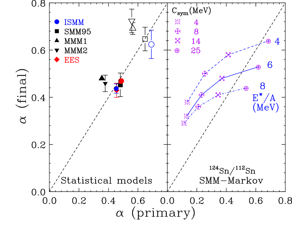
Figure 9: Effect of sequential decays on the isoscaling parameter, $\alpha$. Left panel shows the results of the statistical models studied in this work where the $C_{sym}$ in the models assume a constant value of about 25 MeV and $E*/A=4$ MeV. Right panel shows the results from the microcanonical version of SMM with Markov-chain where $C_{sym}$ varies from 4 (burst symbols), 8 (crosses), 14 (X symbols) and 25 (circular symbols) MeV and $E*/A$ varies from 4 (dashed line), 6 (solid line) and 8 (dot-dashed line).

III.5 Fluctuations of isotope yield ratio temperatures

Ideally, a model should predict isotope cross-sections such as those shown in the right panels of Fig. 5. All model comparisons involve the production of primary fragments and their decays. To disentangle the two parts of the calculations from the final fragments and to evaluate the sequential decay portion of the calculations, we need another observable that is mainly sensitive to the structural decay information, an important ingredient in sequential decay models. It has been shown that the fluctuations observed in the isotope yield temperatures are sensitive to the sequential decay information ref2 ; ref40 .

The isotope yield ratio thermometer is defined as albergo

$$\mathrm{T}=\frac{B}{\ln{a\cdot R}}$$ (3)

where $B$ is a binding energy parameter, $a$ is the statistical factor that depends on statistical weights of the ground state nuclear spins and $R$ is the ground state isotope yield ratio,

$$\mathrm{R}=\frac{Y(A_{1},Z_{1})/Y(A_{1}+1,Z_{1})}{Y(A_{2},Z_{2})/Y(A_{2}+1,Z_{2})}$$ (4)

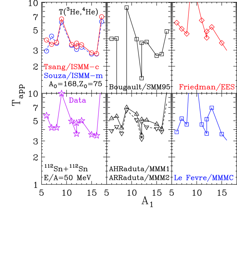
Figure 10: Isotopic temperatures $T(^{3}$He,⁴He) constructed from different isotope pairs in the numerator of Eq. (4) and the ratios of $Y(^{3}$He)/$Y(^{4}$He) in the denominators are plotted as a function of $A_{1}$. The data ref11b are plotted in the bottom left corner for reference. Models with similar decay codes such as ISMM-c and ISMM-m (top left panel) and MMM1 and MMM2 (bottom middle panel) are plotted together.

In this section, our discussion is mainly focused on using $T$ as a tool to evaluate the modeling of sequential decays. More details about using $T$ as the temperature of the freeze-out source can be found in ref. ref31 . It is possible to construct many different thermometers from various combinations of the isotope yields using Eqs. (3) and (4) ref40 . In the grand-canonical approximation, if all fragments are produced directly in their ground states, these temperatures should all have the same value as the temperature of the initial system. Experimentally, we see large fluctuations of these isotope yield temperatures ref40 ; ref41 ; ref42 , i.e. $T$ depends on the specific combinations of isotopes used in Eq. (4). Without sequential decay corrections, the measured temperature is not the source temperature. Because of the fluctuations, the experimental measured temperatures are usually called $T_{app}$ as denoted in Fig. 10. As an example, we show $T(^{3}$He,⁴He) constructed with $Y(^{3}$He) and $Y(^{4}$He) yields in the denominators ($A_{2}$=3, $Z_{2}$=2) but different isotope pairs in the numerators of Eq. (4). Specifically, we will examine eleven $T(^{3}$He,⁴He) thermometers constructed with the yields of the following isotope pairs in the numerators:
$Y(^{6}$Li)/$Y(^{7}$Li), $Y(^{7}$Li)/$Y(^{8}$Li), $Y(^{8}$Li)/$Y(^{9}$Li),
$Y(^{9}$Be)/$Y(^{10}$Be), $Y(^{11}$B)/$Y(^{12}$B), $Y(^{12}$B)/$Y(^{13}$B),
$Y(^{12}$C)/$Y(^{13}$C), $Y(^{13}$C)/$Y(^{14}$C), $Y(^{15}$N)/$Y(^{16}$N),
$Y(^{16}$O)/$Y(^{17}$O), and $Y(^{17}$O)/$Y(^{18}$O).

These isotope pairs are chosen because the data for the central collisions of ¹¹²Sn+¹¹²Sn at $E/A$=50 MeV are available ref2 ; ref18 . $T(^{3}$He,⁴He) are constructed from the values of $a$ and $B$ listed in ref. ref11b . These temperatures are plotted as a function of $A_{1}$ in the lower left panel of Fig. 10. To get a glimpse of how well different evaporation codes which are coupled to the statistical multifragmentation models listed in Table 1 simulate sequential decays, $T(^{3}$He,⁴He) constructed with the final fragments produced from the different statistical models are plotted in the remaining panels of Fig. 10. Instead of assuming a constant value, $T(^{3}$He,⁴He) fluctuates in all models. This suggests that decays to low lying excited states occur. If a significant fraction of the particles de-excite to the gamma levels below the particle decay thresholds, the ground state cross-sections are modified. Such contaminations may have caused the higher temperatures determined from the yields of ⁹Be ($A_{1}=9,Z_{1}=4$) and ¹⁸O ($A_{1}+1=18,Z_{1}=8)$ which have several low lying excited states below the neutron thresholds. Similar fluctuations have been observed in different reaction systems at different temperatures ref11b ; ref40 ; ref41 ; ref42 . They mainly originate from the detailed structure of the excited states. Thus the fluctuations in the isotope temperature provide a sensitive tool to evaluate whether proper decay levels have been taken into account in a code.

These fluctuations are mainly determined by the sequential decay portion of the code. Models with the same decay codes exhibit nearly the same fluctuations even though the primary IMF multiplicities and mass distributions are different. For example, different freeze-out assumptions used in the two MMM codes result in very different mean IMF multiplicities (Fig. 1) and different residue distributions (Fig. 2). However, the isotope yield ratio temperatures have the same trends (bottom middle panel) suggesting that sequential decays mask off some initial differences in the source. The fluctuations in ISMM-c and ISMM-m are similar (top left panel). Since the MSU-decay code incorporates the most structural information for the light fragments ($Z<$15), $T(^{3}$He,⁴He) determined from the two ISMM codes that employ the MSU-decay as after-burners reproduce the trend of the experimental fluctuations the best (top left panel). However, $T(^{3}$He,⁴He) is lower than the input temperature of 4.7 MeV suggesting that the sequential decay effects on the initial temperature can be substantial. As ⁹Li isotopes are not produced in the SMM95 code, the temperatures involving this isotope drops (top middle panel). Individual temperature values do not agree among models even though the initial input to the fragmenting source is the same. The differences in the isotope yield ratio temperatures probably reflect the difference in the decay codes.

IV Evaporation models:

Before comparing calculated results with data, all hot fragments produced in any models must undergo decay. Unfortunately the task to simulate sequential decays has proved to be rather difficult due to the lack of complete information on nuclear structures and level densities. In this section, we compare five sequential decay models (see Table 1) that have been used in many studies. The bench mark systems are 1) $A_{0}$=168, $Z_{0}$=75 and 2) $A_{0}$=186, $Z_{0}$=75. The excitation energy is 2 MeV per nucleon. For brevity, we only discuss three observables, which illustrate the differences in the codes.

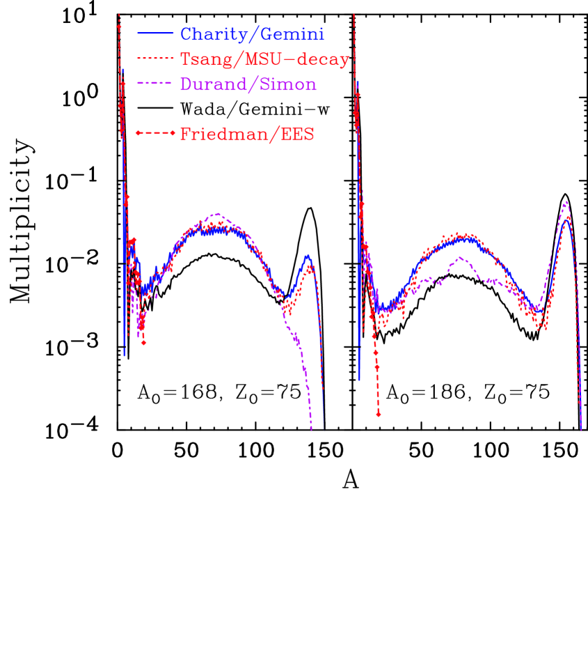
Figure 11: Predicted mass distributions from the five evaporation codes listed in Table 1 for the neutron-deficient system 1 (left panel) and neutron-rich system 2 (right panel).

IV.1 Mass distributions

Figure 11 shows the mass distributions from the decay of the $A_{0}$=168, $Z_{0}$=75 system (left panel) and $A_{0}$=186, $Z_{0}$=75 system (right panel). Contrary to the near exponential decrease of the production of fragments with increasing mass in multifragmentation processes (Fig. 2), most evaporation models de-excite by emitting LCPs, leaving a residue. Fission is also a significant de-excitation mode in this mass region, resulting in a hump at about 10 mass units less than $A_{0}$/2. The inability of the EES model (symbols joined by dashed lines) to track fragments larger than A=20 results in the artificial truncation of the mass distribution. Since the MSU-decay uses Gemini to decay fragments with $Z>$15, results from Gemini (solid line) and MSU-decay models (dotted line) are very similar. In principle, Gemini-w (dashed line) should be the same as Gemini. However, an older version of Gemini was incorporated and Germini-w gives much larger residue cross-sections and correspondingly smaller fission fragment and IMF cross-sections. The event generator code, SIMON (dot-dashed line) has very different mass distributions than the other codes, e.g. it does not produce residues in the $A_{0}$=168, $Z_{0}$=75 system (left panel).

IV.2 Isoscaling

Primary fragments produced from nearly all statistical multifragmentation codes observe isocaling, rigorously. However, isoscaling is not well observed over a large range of secondary fragments. For this reason, we limit the number of isotopes to three for each element, similar to those measured in experimental data. We use this observable to examine the differences between different models in Fig. 12. The symbol convention of Figs. 7 and 8 is used, i.e. symbols are yield ratios and lines are best fits. Isoscaling is reasonably reproduced except for SIMON. For the MSU-dacay and EES (not shown) decays, the results are similar to those of ISMM and EES calculations shown in Fig. 8. Except for ⁶He yield ratios, Gemini exhibits very good isoscaling. The isoscaling from Gemini-w fragments is not as good. The same problems that cause SIMON to produce different mass distributions could be the cause for the non-observation of isoscaling behavior.

IV.3 Fluctuation of isotope yield ratio temperatures

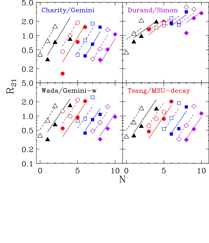
Figure 12: Predicted ratios, $R_{21}(N,Z)=Y_{2}(N,Z)/Y_{1}(N,Z)$ of fragments evaporated from system 2 and system 1. Each panel presents the results from one model calculation. The results from the EES model are not plotted here as they are similar to those shown in Fig. 8.

In Fig. 13, we show T(³He, ⁴He) constructed with Y(³He) and Y(⁴He) yields in the denominators ($A_{2}=3,Z_{2}$=2) but different isotope pairs in the numerators of Eq. (4) as discussed in Section 3.5. For reference, the Sn data are plotted in the lower left panel of Fig. 13 as a function of $A_{1}$. As light-particle structure information has been included in EES, Gemini, and MSU-decay codes, they reproduce the fluctuations observed experimentally rather well as shown in the top three panels in Fig. 13. On the other hand, SIMON and Gemini-w do not reproduce the general trends suggesting that the sequential decays are not properly taken into account in these codes.

Most of the isotope yield ratio temperatures from EES, Gemini and MSU-decay calculations are below 4 MeV, the input temperature of the source. Sequential decay effects are expected to reduce the initial temperature. It is interesting to note that of the three models that reproduce the fluctuations, the average temperature is the highest for the EES model and lowest for the MSU-decay model. This can be explained by the amount of structural information included in individual models. EES incorporates only a few low lying excited states while the MSU-decay model incorporates most of the experimental level information for nuclei with Z$<$15. The availability of a large number of decay levels in the latter code reduces the ground-state cross-sections more than in other calculations. This suggests that even at low excitation energy (2 MeV), sequential decays still significantly affect isotope yields.

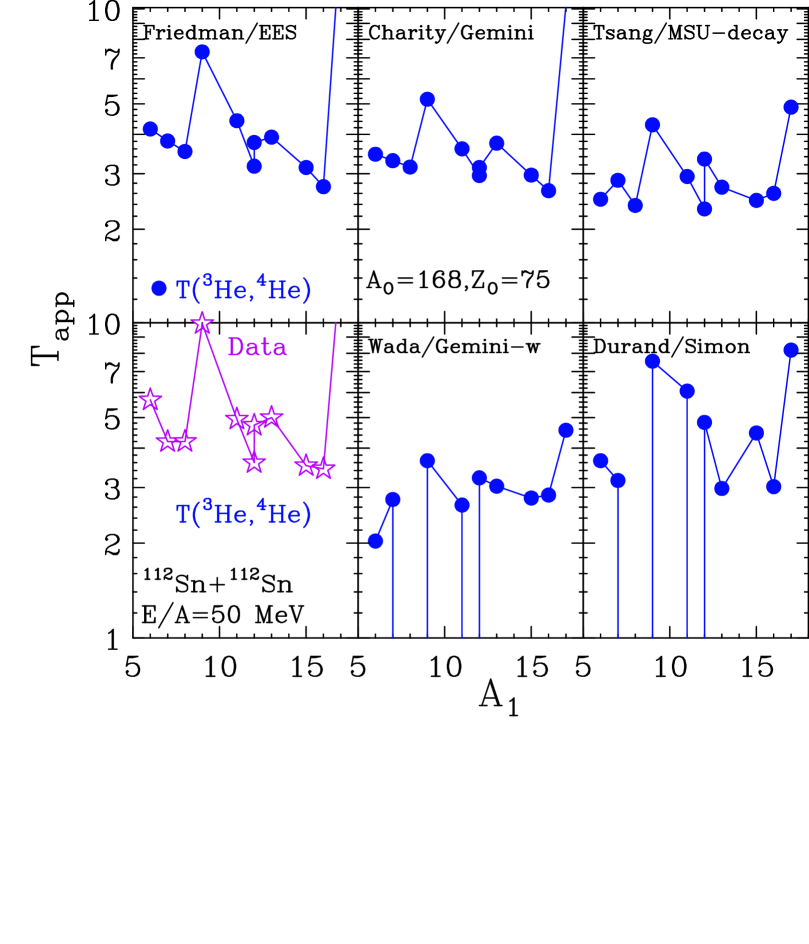
Figure 13: Isotopic temperature $T(^{3}$He,⁴He) plotted as a function of $A_{1}$. For reference, the data ref11b are plotted in the bottom left corner.

V Summary and Conclusions

In summary, we have made comparisons of experimental observables using ten statistical multifragmentation codes. The general trends are similar among models suggesting that these models can provide important physical insights for the primary fragments and multifragmentation process. However, details in any single observable differ between models. The largest differences are observed in raw observables such as individual isotope yields, mass and charge distributions while the mean values of an observable such as IMF multiplicity, the mean fragment asymmetry $<N/Z>$ or mean mass $<A>$ of an element do not show as large differences. The effects of sequential decays on isoscaling parameters are not well understood.

As sequential decay codes are important to both dynamical and statistical models, we also compare five widely used codes. Relatively accurate structural information and experimental masses are required in evaporation models to reproduce the fluctuations of isotope yield temperatures. Such sensitivity allows one to evaluate the sequential decay properties of the evaporation codes.

The observables studied here are by no means an exhaustive list. However, these observables, which can be constructed easily from the isotope yields, provide important bench-marks to test any multifragmentation models or evaporation codes that describe sequential decays.

VI Acknowledgment

The authors wish to thank Dr. C. Bertulani for his help in the beginning of this project. MBT acknowledges the support of the National Science Foundation under Grant No. PHY-01-10253.

References

- (1) S. Das Gupta, A.Z. Mekjian and M.B. Tsang, Adv. Nucl. Phys. 26, (2001) 91 and references therein
- (2) C.B. Das, S. Das Gupta, W.G. Lynch, A.Z. Mekjian, M.B. Tsang Phys. Rep. 406, (2005) 1
- (3) J. Randrup and S.E. Koonin, Nucl. Phys. A356, (1981) 223
- (4) J.P. Bondorf, A.S. Botvina, A.S. Iljinov, I.N, Mishustin, and K. Sneppen, Phys. Rep. 257, (1995) 133, and refs. therein
- (5) D.H.E. Gross, Phys. Rep. 279, (1997) 119, and refs. therein
- (6) W.A. Friedman and W.G. Lynch, Phys. Rev. C 28, (1983) 16
- (7) W.A. Friedman, Phys. Rev. Lett. 60, (1988) 2125
- (8) W.A. Friedman, Phys. Rev. C 42, (1990) 667
- (9) A.S. Botvina, A.S. Iljinov, I.N. Mishustin, J.P. Bondorf, R. Donangelo, and K. Sneppen, Nucl. Phys. A475, (1987) 663
- (10) J.P. Bondorf et. al., Nucl. Phys. A443, (1985) 321; ibid. A444, (1985) 460; ibid. A448, (1986) 753; K. Sneppen, Nucl. Phys. A470, (1987) 213
- (11) A.S. Botvina, A.S. Iljinov and I.N. Mishustin, Sov. J. Nucl. Phys. 42, (1985) 712
- (12) G.F. Bertsch, Am. J. Phys., 72, (2004) 983
- (13) S.R. Souza, W.P. Tan, R. Donangelo, C.K. Gelbke, W.G. Lynch and M.B. Tsang, Phys. Rev. C 62, (2000) 064607
- (14) W.P. Tan, S.R. Souza, R.J. Charity, R. Donangelo, W.G. Lynch, M.B. Tsang, Phys. Rev. C 68, (2003) 034609
- (15) Al.H. Raduta and Ad.R. Raduta, Phys. Rev. C 65, (2002) 054610
- (16) A. Le Fèvre et al., Nucl. Phys. A735, (2004) 219
- (17) Ph. Chomaz and F. Gulminelli, Phys. Rev. Lett. 82, (1999) 1402
- (18) D. Hahn and H. Stöcker, Nucl. Phys. A 476, (1988) 718
- (19) C.E. Aguiar, R. Donangelo, and S.R. Souza, Phys. Rev. C 73, (2006) 024613
- (20) T.X. Liu et. al., Phys. Rev. C 69, (2004) 014603
- (21) H.S. Xu et. al., Phys. Rev. Lett. 85, (2000) 716
- (22) see, e.g., A.S. Botvina and I.N. Mishustin, contribution to this volume
- (23) V.F. Weisskopf, D. H. Ewing, Phys. Rev. 57, (1940) 472
- (24) M. Colonna, private communications
- (25) R.J. Charity et al., Nucl. Phys. A483, (1988) 371,
- (26) K. Yuasa-Nakagawa et al., Phys. Rev. C 53, (1996) 997
- (27) J. Cibor et al., Phys. Rev. C 55, (1997) 264
- (28) R. Wada et al., Phys. Rev. C 62, (2000) 34601; Phys. Rev. C 69, (2004) 44610
- (29) D. Durand, Nucl. Phys. A541, (1992) 266
- (30) J.D. Frankland et al., Nucl. Phys. A689, (2001) 940
- (31) D. Lacroix, A. Van Lauwe, D. Durand, Phys. Rev. C 69, (2004) 054604
- (32) F. Gulminelli and Ph. Chomaz, Phys. Rev. C 71, (2005) 054607
- (33) J. Konopka, H. Graf, H. Stöcker, W. Greiner, Phys. Rev. C 50, (1994) 2085
- (34) Hongfei Xi et al., Z. Phys. A 359, (1997) 397; Eur. Phys. J. A 1, (1998) 235 (the second reference is an erratum to the first)
- (35) A. Kelić, J.B. Natowitz, K.-H. Schmidt, contribution to this volume
- (36) G.J. Kunde et al., Phys. Rev. Lett. 77, (1996) 2897
- (37) W.D. Myers and W.J. Swiatecki, Nucl. Phys. 81, (1966) 1; Ark. Fiz. 36, (1967) 343
- (38) M.B. Tsang, W.A. Friedman, C.K. Gelbke, W.G. Lynch, G. Verde, H.S. Xu, Phys. Rev. Lett. 86, (2001) 5023
- (39) M.B. Tsang et. al., Phys. Rev. C 64, (2001) 054615
- (40) A.S. Botvina, O.V. Lozhkin and W. Trautmann, Phys. Rev. C 65, (2002) 044610
- (41) A. Ono, P. Danielewicz, W.A. Friedman et al., Phys. Rev. C 68, (2003) 051601(R)
- (42) M. Colonna, M.B. Tsang, contribution to this volume
- (43) E. Geraci et al., Nucl. Phys.A732, (2004) 173.
- (44) A. Le Fèvre, G. Auger, M.L. Begemann-Blaich et al., Phys. Rev. Lett. 94, (2005) 162701
- (45) A. Ono et al., arXiv:nucl-ex/0507018
- (46) M.B. Tsang, W.G. Lynch, H. Xi and W.A. Friedman, Phys. Rev. Lett. 78, (1997) 3836
- (47) S. Albergo et. al, Nuovo Cimento A89, (1985) 1
- (48) M.J. Huang et al., Phys. Rev. Lett. 78 (1997) 1648
- (49) H. Xi et. al, Phys. Lett. B431, (1998) 8