Shell structure underlying the evolution of quadrupole collectivity in ³⁸S and ⁴⁰S probed by transient-field $g$-factor measurements on fast radioactive beams.

Abstract

The shell structure underlying shape changes in neutron-rich nuclei between $N=20$ and $N=28$ has been investigated by a novel application of the transient field technique to measure the first-excited state $g$ factors in ³⁸S and ⁴⁰S produced as fast radioactive beams. Details of the new methodology are presented. In both ³⁸S and ⁴⁰S there is a fine balance between the proton and neutron contributions to the magnetic moments. Shell model calculations which describe the level schemes and quadrupole properties of these nuclei also give a satisfactory explanation of the $g$ factors. In ³⁸S the $g$ factor is extremely sensitive to the occupation of the neutron $p_{3/2}$ orbit above the $N=28$ shell gap as occupation of this orbit strongly affects the proton configuration. The $g$ factor of deformed ⁴⁰S does not resemble that of a conventional collective nucleus because spin contributions are more important than usual.

I Introduction

In a recent Letter Davies et al. (2006a) we presented the first application of a high-velocity transient-field (HVTF) technique Stuchbery (2004) to measure the $g$ factors of excited states of neutron-rich nuclei produced as fast radioactive beams. Questions on the nature and origins of deformation between $N=20$ and $N=28$ were addressed by measuring the $g$ factors of the 2${}_{1}^{+}$ states in ${}^{38}_{16}$S₂₂ and ${}^{40}_{16}$S₂₄. Fig. 1 shows the relevant part of the nuclear chart and indicates the primary beams used to produce the isotopes of interest. In the present paper we give a more comprehensive description of the experiment and discuss the interpretation in greater detail. A more technically-oriented discussion of the new technique will be published elsewhere Davies et al. (2006b).

Figure 1: (Color online) Region of the nuclear chart indicating the primary beam isotopes ⁴⁰Ar and ⁴⁸Ca used to produce the ³⁸S and ⁴⁰S secondary beams (red). The $N=20,28$ closed shells are shown outlined in black. Stable isotopes are shaded (blue).

Figure 2: Previously-measured $E(2^{+})$ and $B(E2)$ values for the sulfur isotopes Raman et al. (2001).

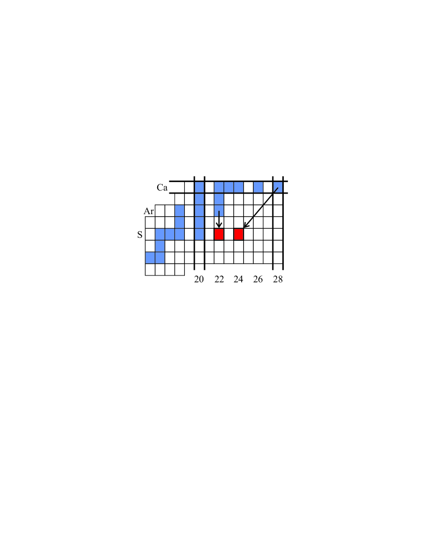
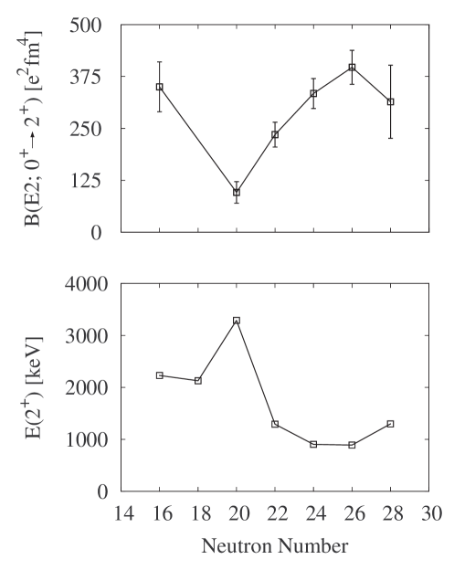
Figure 2 shows the 2${}^{+}_{1}$ excitation energies and the $B(E2;0^{+}_{1}\rightarrow 2^{+}_{1})$ values for the sulfur isotopes. It is apparent from the reduction in the excitation energies of the 2${}^{+}_{1}$ states and the increase in $B(E2)$ values that the neutron rich isotopes between $N=20$ and $N=28$ develop collective features. Furthermore, the $N=28$ nucleus ${}^{44}_{16}$S₂₈ does not have the high 2${}^{+}_{1}$ energy and small $B(E2)$ like the closed-shell $N=20$ isotope ${}^{36}_{16}$S₂₀. The data in Fig. 2 together with additional information on the low-excitation level structures imply that the even sulfur isotopes between $N=20$ and $N=28$ undergo a transition from spherical at ${}^{36}_{16}$S₂₀, to prolate deformed in ${}^{40}_{16}$S₂₄ and ${}^{42}_{16}$S₂₆, and that the $N=28$ nucleus ${}^{44}_{16}$S₂₈ appears to exhibit collectivity of a vibrational character Scheit et al. (1996); Glasmacher et al. (1997); Winger et al. (2001); Sohler et al. (2002). However the evolution of collective features in these nuclei has underlying causes that remain unclear. Some have argued that a weakening of the $N=28$ shell gap is important Sohler et al. (2002); Werner et al. (1994), while others have opined that the effect of adding neutrons to the $f_{7/2}$ orbit is primarily to reduce the proton $s_{1/2}$-$d_{3/2}$ gap and that a weakening of the $N=28$ shell gap is not needed to explain the observed collectivity near ⁴⁴S Cottle and Kemper (1998). There have been several theoretical studies discussing the erosion of the $N=28$ shell closure and the onset of deformation (e.g. Refs. Rodríguez-Guzmán et al. (2002); Caurier et al. (2004) and references therein). To help resolve questions on the nature and origins of deformation between $N=20$ and $N=28$, we have used a novel technique to measure the $g$ factors of the 2${}_{1}^{+}$ states in ${}^{38}_{16}$S₂₂ and ${}^{40}_{16}$S₂₄.

The remainder of the paper is arranged as follows: Section II describes the experimental procedures including radioactive beam production, targets and apparatus. The experimental results and details of the data analysis are given in Section III. Our shell model calculations are presented and discussed in Section IV.

II Experimental procedures

II.1 Overview

The experiments reported here use transient fields to study neutron-rich nuclei produced as radioactive beams by fast fragmentation. In our approach the nuclear states of interest are excited and aligned by intermediate-energy Coulomb excitation Glasmacher (1998). The nucleus is then subjected to the transient field in a higher velocity regime than has been used previously for moment measurements, which causes the nuclear spin to precess. Finally, the nuclear precession angle, to which the $g$ factor is proportional, is observed via the perturbed $\gamma$-ray angular correlation measured using a multi-detector array. It is important to note that the transient-field technique has sensitivity to the sign of the $g$ factor, which in itself can be a distinguishing characteristic of the state under study, since the signs of the spin contributions to the proton and the neutron $g$ factors are opposite.

The transient field (TF) is a velocity-dependent magnetic hyperfine interaction experienced by the nucleus of a swift ion as it traverses a magnetized ferromagnetic material Benczer-Koller et al. (1980); Speidel et al. (2002). For light ions ($Z\lesssim 16$) the maximum TF strength is reached when $v=Zv_{0}$, i.e. the ion velocity $v$ matches the $K$-shell electron velocity $Zv_{0}$ ($v_{0}=c/137$, Bohr velocity). Since the transient field arises from polarized electrons carried by the moving ion its strength falls off as the ion velocity exceeds $Zv_{0}$ and the ion becomes fully stripped; a transient-field interaction will not occur for fast radioactive beams with energies near 100 MeV/nucleon until most of that energy is removed. Thus slowing the fast fragment beams to velocities where the transient field can be effective is an essential feature of the measurement.

II.2 Radioactive beam production and properties

The experiment was conducted at the Coupled Cyclotron Facility of the National Superconducting Cyclotron Laboratory at Michigan State University. Secondary beams of ³⁸S and ⁴⁰S were produced from 140 MeV/nucleon primary beams of ⁴⁰Ar and ⁴⁸Ca, respectively, directed onto a $\sim 1$ g/cm^{2 9}Be fragmentation target at the entrance of the A1900 fragment separator Morrissey et al. (2003). An acrylic wedge degrader 971 mg/cm² thick and a 0.5% momentum slit at the dispersive image of the A1900 were employed. The wedge degrader allowed the production of highly pure beams and also reduced the secondary beam energy to $\sim 40$ MeV/nucleon. Further details of the radioactive beams are given in Table 1. The ³⁸S (⁴⁰S) measurement ran for 81 (68) hours. The 40 MeV/nucleon beams were made incident upon a target consisting of contiguous layers of Au and Fe, 355 mg/cm² thick and 110 mg/cm² thick, respectively.

Table 1: Production and properties of radioactive beams.

Primary beam		Secondary beam
Ion	Intensity	Ion	$E$	Intensity	Purity
	(pnA)		(MeV)	(pps)	(%)
40Ar	25	38S	1547.5	$2\cdot 10^{5}$	$>99$
48Ca	15	40S	1582.5	$2\cdot 10^{4}$	$>95$

II.3 Target design and test

Prior to the transient-field measurement a test run was performed to ensure that the fast fragment beams at $\sim 40$ MeV/nucleon would be slowed to the appropriate velocity regime in the target layers and emerge from the target for downstream detection without severe energy straggling. A 1540 MeV ³⁸S beam was used for this purpose.

Three targets were mounted, in turn, on a rotating target ladder and the energy distribution of the emerging ions was measured with a 980 $\mu$m PIN detector placed 41 cm downstream of the target. The targets were: (i) the 355 mg/cm² Au foil alone, (ii) the Au (355 mg/cm²) + Fe (100 mg/cm²), and (iii) the Au (355 mg/cm²) + Fe (110 mg/cm²) target, which was subsequently chosen for the $g$-factor measurement. The angle between the target and the beam was varied to effectively increase the target thickness. The transmission of the beam through the target and the energy distribution of the transmitted ions were measured using the PIN detector. These measurements indicated that the Ziegler (1985) stopping powers Ziegler et al. (1985) for sulfur in Au and Fe targets were accurate to about $\pm 5\%$, although they tend to underestimate the stopping in the Au layer of the target and overestimate the stopping in the Fe layer.

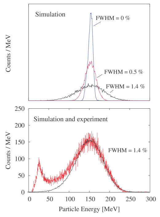
The effect of the energy-width of the radioactive beam on the spectrum of the emergent ions is examined in Fig. 3, which compares the particle spectrum measured in the test run for the Au + Fe (100 mg/cm²) target with Monte Carlo simulations made with the code GKINT_MCDBLS Stuchbery et al. (2006). In the simulations the energy spread of the beam was treated as a Gaussian distribution with its width specified by the Full Width at Half Maximum (FWHM). In the case shown in Fig. 3 the sulfur fragments emerged with energies in the range from $\sim 80$ MeV to $\sim 200$ MeV. A similar post-target energy distribution was observed in the $g$ factor measurements where both the beam energy and the thickness of the Fe layer were increased slightly. It is evident from Fig. 3 that most of this energy-spread stems from the energy width of the radioactive beam, which is determined largely by the momentum acceptance, $\Delta p/p=0.5\%$ (FWHM), set at the dispersive image slits of the A1900 spectrometer.

Figure 3: (Color online) Spectrum of 1540 MeV ³⁸S beam particles after passing through 355 mg/cm² of Au followed by 100 mg/cm² of Fe. The upper panel shows simulations that examine the effect of the energy-width of the ³⁸S beam, which is assumed to have a Gaussian distribution about 1540 MeV with a specified Full Width at Half Maximum (FWHM). These simulated spectra all have the same number of events. The experimental spectrum in the lower panel agrees with the simulations which assume the beam energy has a Gaussian distribution with a FWHM of 1.4% (i.e. a standard deviation of 0.5%). The equivalent momentum width is $\Delta p/p=0.7\%$.

II.4 Apparatus

Figure 4 shows the experimental arrangement. The radioactive beams were delivered onto the Au + Fe target, which had dimensions $30\times 30$ mm². The target was held between the pole tips of a compact electromagnet that provided a magnetic field of 0.11 T, sufficient to fully magnetize the Fe layer. As the iron layer of the target is much thicker than those typically used in transient-field $g$-factor measurements, the magnetization of a piece was measured using the Rutgers Magnetometer Piqué et al. (1989). Fields of 0.062 T were sufficient to ensure saturation. To minimize possible systematic errors, the external magnetic field was automatically reversed every 600 s.

Table 2 summarizes the properties of the 2${}^{+}_{1}$ states and the key aspects of the energy loss of the sulfur beams in the target, applicable for the $g$ factor measurements. The high-$Z$ Au target layer serves to enhance the Coulomb excitation yield and slow the projectiles to under 800 MeV, while the thick iron layer results in a long interaction time with the transient field, maximizing the spin precession. The energies $\langle E_{i}\rangle$, with which the sulfur ions enter the iron layer, were calculated taking into account the energy loss measurements for the Au layer alone, while the energies $\langle E_{e}\rangle$, with which the ions emerge from the iron layer into vacuum, were determined from the Doppler shifts observed in the $g$-factor measurements.

Table 2: Nuclear parameters and reaction kinematics. $B(E2)\!\!\uparrow\ =B(E2;0^{+}_{\rm gs}\rightarrow 2^{+}_{1})$. $\langle E_{i,e}\rangle$ and $\langle v_{i,e}\rangle$ are the ion kinetic energies and velocities at the entrance and exit of the iron layer. The effective transient-field interaction time $t_{\rm eff}$ is evaluated for ions that decay after leaving the target.

Isotope	E(2${}^{+}_{1}$)	$B(E2)\uparrow$	$\tau$(2${}^{+}_{1}$)	$\langle E_{i}\rangle$	$\langle E_{e}\rangle$	$\langle v_{i}/Zv_{0}\rangle$	$\langle v_{e}/Zv_{0}\rangle$	$t_{\rm eff}$
	(keV)	(e2fm4)	(ps)	(MeV)	(MeV)			(ps)
38S	1292	235(30)	4.9	762	123	1.75	0.71	2.98
40S	904	334(36)	21	782	145	1.73	0.75	2.99

Figure 4: (Color online) Overhead view of the SeGA detectors and side view of the target chamber showing the magnet, target and phoswich detector. Projectiles were detected in the downstream phoswich detector.

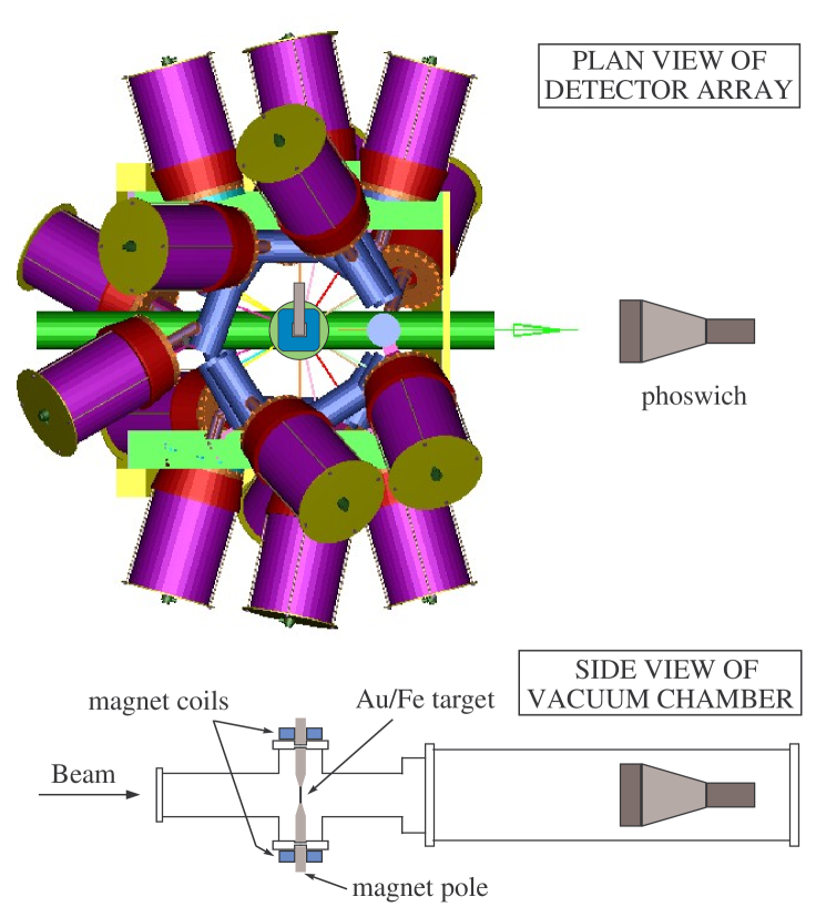
Projectiles scattered forward out of the target were detected with a 15.24 cm diameter plastic scintillator phoswich detector placed 79.2 cm downstream of the target position. The phoswich detector consisted of a 750 $\mu$m layer of fast BC-400 scintillator and a 5.08 cm layer of slow BC-444 scintillator. The maximum scattering angle, 5.5^∘, limits the distance of closest approach to near the nuclear interaction radius in both the Au and Fe target layers. Positioning the particle detector downstream also lowers the exposure of the $\gamma$-ray detectors to the radioactive decay of the projectiles.

While the sulfur fragments do not penetrate beyond the fast scintillator, the slow scintillator helps discriminate against more penetrating radiation such as light ions produced in the secondary target, or accompanying the beam, and $\beta$ decays in the phoswich from the decay of the implanted radioactive beam. Along with the fast-slow particle identification information from the phoswich, the particle time-of-flight was also recorded with respect to the cyclotron RF. Triggers from the radioactive decay of the beam particles, which are much lower in energy than the beam particles, were minimized by raising the threshold of the phoswich discriminator.

For the ³⁸S run, a circular Pb mask was placed on the phoswich detector to block particles in the range $0^{\circ}\leq\theta\leq 2.5^{\circ}$ and hence lower the count rate by excluding those scattering angles where the Rutherford cross section is large but the Coulomb excitation cross section is small. The mask helped reduce random particle-$\gamma$ coincidences and pileup events in the phoswich detector. No mask was used for the ⁴⁰S run since the particle rate was low enough for pileup to be negligible.

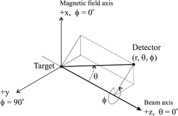
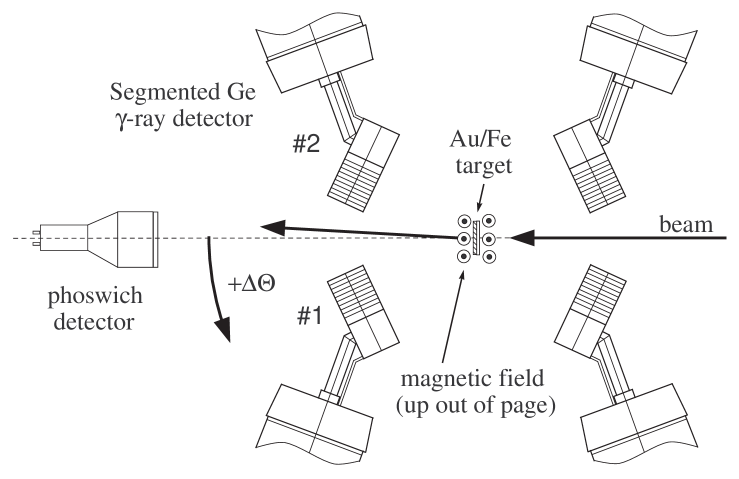
To detect de-excitation $\gamma$ rays, the target chamber was surrounded by 14 HPGe detectors of the Segmented Germanium Array (SeGA) Mueller et al. (2001). The SeGA detectors were positioned with the crystal centers 24.5 cm from the target position. Six pairs of detectors were fixed at symmetric angles $(\pm\theta,\phi)=(29^{\circ},90^{\circ})$, $(40^{\circ},131^{\circ})$, $(60^{\circ},61^{\circ})$, $(139^{\circ},46^{\circ})$, $(147^{\circ},143^{\circ})$, and $(151^{\circ},90^{\circ})$, where $\theta$ is the polar angle with respect to the beam axis and $\phi$ is the azimuthal angle measured from the vertical direction, which coincides with the magnetic field axis. Figure 5 indicates the coordinate frame and definitions of the angles. To make a connection with the notation used for conventional transient-field measurements Benczer-Koller et al. (1980); Speidel et al. (2002), the locations of the pair of detectors at the spherical polar angles $(\theta,\phi)$ and $(\theta,\phi+180^{\circ})$ are written as $(\pm\theta,\phi)$; thus if $(+\theta,\phi)=(|\theta|,\phi)$, then $(-\theta,\phi)=(|\theta|,\phi+180^{\circ})$. Each $\pm\theta$ pair is in a plane that passes through the center of the target.

Two additional detectors were placed at $(\theta,\phi)=(90^{\circ},112^{\circ})$ and $(24^{\circ},0^{\circ})$ to assist the measurement of the angular correlation. All 14 detectors were used to measure the $\gamma$-ray angular correlations concurrently with the precessions. Since the precession angles are small, the unperturbed angular correlation can be reconstructed by adding the data for the two directions of the applied magnetic field.

Figure 5: Relation between beam axis, magnetic field axis, and the coordinate systems used in the present experiment and its analysis.

The positions of the SeGA detectors with respect to the target position were measured to an accuracy of 2 mm using a theodolite system. This information was used to find the actual crystal locations in conjunction with the SeGA crystal segment positions measured by Miller et al. Miller et al. (2002). The 32-fold segmentation of the detectors improves the position determination of the $\gamma$ ray from the entire crystal length (8 cm) to near the segment length (1 cm), which is needed for Doppler corrections due to the high velocity of the emitting nuclei. The angle of $\gamma$-ray emission was deduced from the position of the detector segment that registered the highest energy deposition. With this algorithm the position resolution is near (but does not reach) the segment length.

The master trigger for the data acquisition was set to record particle-$\gamma$ coincidences as well as down-scaled particle singles. Thirty three energy signals were recorded for each $\gamma$-ray detector, corresponding to the 32 segments and the central contact. To differentiate between the signals from the fast and slow scintillator, the pulse from the phoswich detector was charge-integrated over the whole signal and over the tail (slow) part of the signal in separate QDC channels. Time differences were recorded between the phoswich detector and the $\gamma$-ray detectors. To assist with particle identification, the time-of-flight spectrum was also recorded for particles striking the phoswich detector. Finally, each event included a tag that identified the direction of the external magnetic field.

III Experimental results and analysis

III.1 Particle and $\gamma$-ray spectra

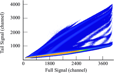
A particle identification plot obtained with the phoswich detector during the ³⁸S measurement is shown in Fig. 6. This spectrum was obtained by plotting the integrated charge for the slow (or tail) part of the phoswich signal versus the integrated charge for the whole signal. Most of the intensity corresponds to the sulfur projectiles. It has a small tail component and therefore occurs in a band located along the full signal axis. The upsloping lines of intensity that deviate from this heavy-ion band are due to low-$Z$ particles that punch through into the slow scintillator. Such ions accompany the beam, probably originating at the acrylic Image-2 wedge in the A1900 spectrometer; they are not predominantly produced in the secondary target.

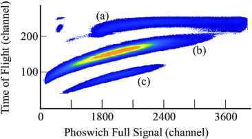
The spectrum in Fig. 7 shows the time-of-flight between the cyclotron RF and the phoswich trigger pulse versus the phoswich energy signal (integration of the full pulse shape). Three distinct features are evident in this spectrum. The upper feature, labeled (a), corresponds to events which cause a large amount of slow scintillation in the phoswich; they are the light particles discussed already. The middle region, labeled (b), corresponds to phoswich events triggered by sulfur projectiles that are in coincidence with $\gamma$ rays, and the lower region, labeled (c), is made up of downscaled phoswich events. (The downscaler module introduces an additional delay that shifts this group of events away from the phoswich-$\gamma$ coincidences.)

Figure 6: (Color online) Phoswich particle identification plot recorded during the ³⁸S run. Pulse-shape discrimination was obtained by plotting the integrated charge for the slow (tail) signal versus the full charge-integrated signal.

Figure 7: (Color online) Time-of-flight (between the cyclotron RF and the phoswich detector) versus the phoswich energy recorded during the ³⁸S run. The labeled features are (a) light particles registered in the slow scintillator, (b) ³⁸S ions in coincidence with $\gamma$ rays, and (c) down-scaled events. See text for further details.

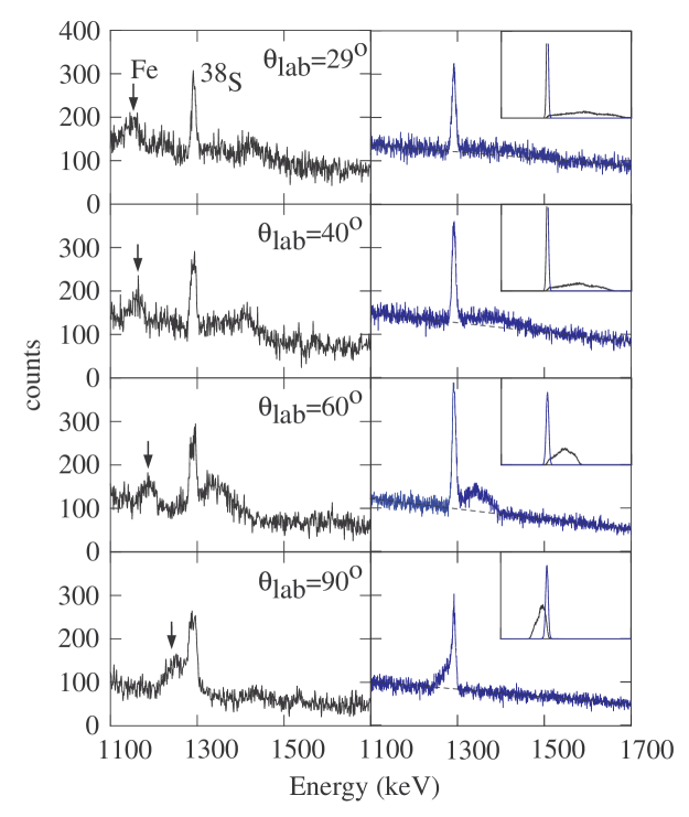
Gamma-ray spectra gated on sulfur recoils were produced and corrected for random coincidences by subtracting spectra gated on the appropriate regions of the particle-$\gamma$ time spectra. Both the particle identification and time-of-flight information from the phoswich were used to select the events of interest. Spectra were also created for each $\gamma$-ray detector and for each direction of the magnetic field (up/down). Examples of the random-subtracted spectra for the lab-frame are given in the upper panels of Fig. 8. From the measured Doppler shift of the deexcitation $\gamma$ rays in the laboratory frame, the average after-target ion velocities were determined to be 0.083 c for ³⁸S and 0.088 c for ⁴⁰S, (i.e. $v/Zv_{0}=$ 0.71 and 0.75, respectively). The velocity distribution of the exiting ⁴⁰S ions was also measured by shifting the phoswich detector by $\pm 15$ cm from its normal position and observing the change in the flight times of the projectiles. These procedures firmly establish that the sulfur ions were slowed through the peak of the TF strength at $Zv_{0}$ into the region where it has been well characterized Speidel et al. (2002); Stuchbery (2004).

Doppler-corrected spectra were also produced using the angular information from the SeGA detector segments and the particle energy information from the phoswich detector on an event-by-event basis, which is essential because of the spread in particle velocities. The lower panels of Fig. 8 show examples of the Doppler-corrected $\gamma$-ray spectra. The peak to background ratio seems to be better for the ⁴⁰S measurement because (i) there are more counts in the ³⁸S measurement, which gives an overall higher count baseline, and (ii) the combination of the higher $\gamma$-ray energy and shorter level lifetime in ³⁸S result in a broader Doppler-corrected peak.

Most of the excited nuclei decay in vacuum after leaving the target material, however for ³⁸S a significant number also decay at higher velocities, extending up to the secondary beam velocity, whilst still within the target. The long Doppler tail becomes almost indistinguishable from background at extreme forward and backward angles, but is clear at $\theta=40^{\circ}$, $60^{\circ}$ and $90^{\circ}$. It was established through Doppler Broadened Line Shape (DBLS) calculations based on a Monte Carlo approach that the angular correlations and nuclear precessions can be determined accurately by an analysis of the vacuum-flight peak alone, without the need to include the Doppler tail. Examples of the DBLS calculations and comparisons with the experimental spectra are shown in Fig. 9. From these spectra it can be seen that the proportion of the $\gamma$-ray peak that corresponds to decays within the target is very small, and only weakly dependent on the detection angle. Note that the present calculations of the lineshapes do not account for the possibility that a $\gamma$-ray event may be assigned to the wrong segment of the detector. Having established that the correct angular correlation and $g$-factor results are obtained by analyzing only the $\gamma$-ray peak, and excluding the tail, no attempt was made to obtain a quantitative fit to the observed $\gamma$-ray line shapes. Further details of these calculations will be given below and elsewhere Stuchbery et al. (2006).

Figure 8: Random-subtracted lab frame (top) and Doppler-corrected (bottom) $\gamma$-ray spectra at $\theta=40^{\circ}$ for ³⁸S (left) and ⁴⁰S (right). The sulfur and iron peaks are labeled. The broad feature to the right of the 1292 keV line is mainly its Doppler tail, due to decays within the target, although there is a contribution from a contaminant line as well. The line at 1238 keV is the $4\rightarrow 2$ transition emitted by ⁵⁶Fe nuclei at rest.

Figure 9: (Color online) Random-subtracted Doppler-corrected $\gamma$-ray spectra from the ³⁸S measurement are shown on the left. The 1238 keV line emitted by ⁵⁶Fe nucleus at rest in the lab frame are shifted towards the ³⁸S peak by the Doppler correction as the detection angle approaches 90^∘. The right panels show simulated spectra used to evaluate the impact of the Doppler Broadened Line Shape on the angular correlation and precession measurements. The insets show the energy range from 1150 to 1550 keV. These simulations, which do not include background, indicate the relative contributions of decays in the target (broad peak) and decays in vacuum (sharp peak), which overlap. The experimental peak is broader than that in the simulations because a simplified model is used for the $\gamma$-ray detectors.

The 2⁺ peak areas averaged 925 counts/detector per field direction for ³⁸S and 400 counts/detector per field direction for ⁴⁰S, in each of the six angle pairs of SeGA detectors used for extracting the precessions.

III.2 Angular correlations and precessions

In the rest frame of the nucleus, the perturbed angular correlation is given by

$$W(\theta,\phi,\pm\Delta\Theta) = 4\pi\sum_{k,q}\frac{a_{k}Q_{k}G_{k}}{(2k+1)}(-1)^{q}$$ (1)

$$\times Y^{k}_{q}(|\Delta\Theta|,\pm\pi/2)Y^{k}_{-q}(\theta,\phi)$$

where $(\theta,\phi)$ are the spherical polar angles at which the $\gamma$-ray is detected and $\pm\Delta\Theta$ is the transient-field precession angle for the two directions of the magnetic field; $k=0,2,4$ and $q$ takes integer values such that $-k\leq q\leq k$. As shown in Fig. 5, the beam direction defines $\theta=0$ and the magnetic-field direction defines $\phi=0$. The unperturbed angular correlation has symmetry about the beam axis and reduces to the $\phi$-independent form:

$$W(\theta)=1+\sum_{k=2,4}a_{k}Q_{k}G_{k}P_{k}(\cos\theta).$$ (2)

The $a_{k}$ coefficients, which depend on the particle detector geometry, the spins of the initial and final nuclear states and the multipolarity of the $\gamma$-ray transition, can be evaluated from the theory of Coulomb excitation Bertulani et al. (2003). The correction factors for the finite solid angles of the $\gamma$-ray detectors, $Q_{k}$, are near unity in the present work. The deorientation coefficients, $G_{k}$, account for the effect of hyperfine fields experienced by ions that recoil into vacuum carrying atomic electrons.

These recoil in vacuum effects were evaluated based on measured charge-state fractions for sulfur ions emerging from iron foils with energies between 92 and 236 MeV Stuchbery et al. (2006). The large free-ion hyperfine interactions of hydrogen- and lithium-like ions Goldring (1982), which quickly reach hard-core values for nuclear lifetimes of a picosecond or more, are dominant. To a good approximation, the deorientation coefficients can be expressed as $G_{k}=1-(Q_{H}+Q_{Li})b_{k}$, where the fraction of ions with one and three electrons is $Q_{H}+Q_{Li}$ and $b_{k}=k(k+1)/(2I+1)^{2}$ for nuclear spin $I$ and $k=2,4$. Using the measured charge-state fractions gives $G_{2}=0.90$ and $G_{4}=0.65$.

The angular correlations were calculated with the program GKINT Stuchbery (2005). For each layer of the target, the code GKINT performs integrals over the solid angle of the particle detector and over the energy loss of the beam in the target. The average $a_{k}$ coefficients, for example, are evaluated as

$$\langle a_{k}\rangle = \frac{2\pi}{\langle\sigma\cdot t_{\rm tgt}\rangle}\int_{0}^{t_{\rm tgt}}\int_{\theta_{p}^{\rm min}}^{\theta_{p}^{\rm max}}a_{k}(\theta_{p},E[z])$$ (3)

$$\times \frac{d\sigma}{d\Omega}(\theta_{p},E[z])\;\sin\theta_{p}d\theta_{p}dz,$$

where

$$\langle\sigma\cdot t_{\rm tgt}\rangle=2\pi\int_{0}^{t_{\rm tgt}}\int_{\theta_{p}^{\rm min}}^{\theta_{p}^{\rm max}}\frac{d\sigma}{d\Omega}(\theta_{p},E[z])\;\sin\theta_{p}d\theta_{p}dz,$$ (4)

where $\frac{d\sigma}{d\Omega}(\theta_{p},E[z])$ denotes the Coulomb excitation cross section as a function of the scattering angle $\theta_{p}$ and the projectile energy $E[z]$, which varies with the depth $z$ through the target layer. The integrals are evaluated numerically using Simpson’s rule. To evaluate other average quantities of interest such as the average energy of excitation, or the average transient-field precession, the quantity to be averaged replaces $a_{k}$ in an expression of the same form as Eq. (3).

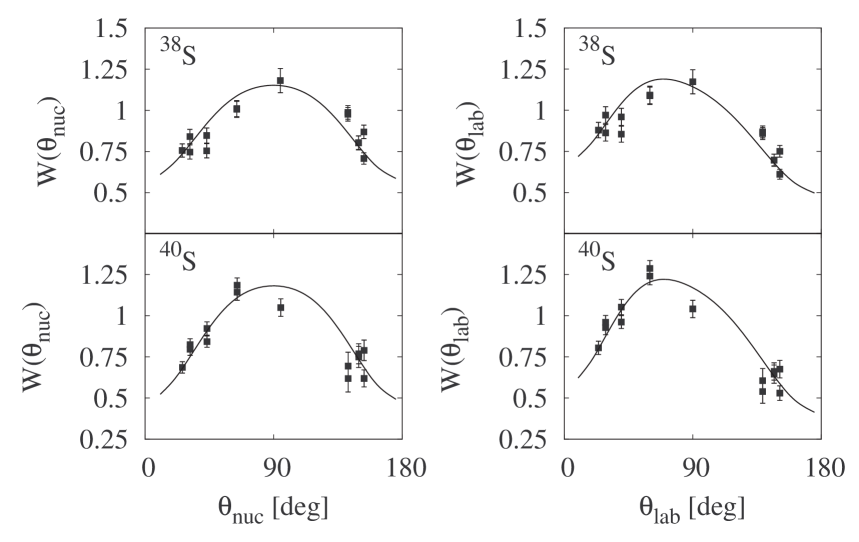
Comparisons between the experimental and theoretical angular correlations are made in Fig 10. To indicate the effect of the Lorentz transformation (see e.g. Stuchbery (2003); Olliver et al. (2003)) the angular correlations are shown in both the laboratory frame and the projectile frame. Good agreement was found between the calculated $\gamma$-ray angular correlations and the data.

Figure 10: Angular correlations for ³⁸S and ⁴⁰S. The left panels show the angular correlation in the frame of the projectile nucleus, while the right panels show the same angular correlations in the lab frame. The Lorentz boost causes a shift in the effective detection angle and an angle-dependent change in the solid angle. Data are normalized to the calculated angular correlation. The difference in anisotropy stems from the alignment produced by Coulomb excitation, which depends on the ratio of $E(2^{+})$ to the beam velocity (i.e. the adiabacity parameter, $\xi$, see Bertulani et al. (2003) and references therein.)

To describe the procedure for the extraction of the nuclear precession angle $\Delta\Theta$ it is helpful to begin with the 4 detectors in the plane through the target that is perpendicular to the magnetic field direction, as illustrated in Fig. 11. For these detectors $\Delta\Theta=\Delta\theta$ and the data analysis is identical to that in a conventional transient-field $g$-factor measurement Benczer-Koller et al. (1980); Speidel et al. (2002); Jakob et al. (1999); Mantica et al. (2001). The magnetic field causes a rotation of the angular correlation pattern around the $x$-axis, with positive precession angles for a right-handed co-ordinate frame in the direction indicated. Thus to first order in $\Delta\Theta$ we have

$$W\uparrow\downarrow=W(\theta\mp\Delta\Theta)\simeq W(\theta)\mp\Delta\Theta\frac{dW}{d\theta},$$ (5)

where the arrows indicate the direction of the external magnetic field. The precession angle is then determined from the double ratio of counts in a pair of detectors for each field direction. Considering, for example, the pair of detectors labeled 1 and 2 in Fig. 11, the relevant experimental double ratio $\rho$ is

$$\rho=\sqrt{\frac{N_{1}\uparrow}{N_{1}\downarrow}\cdot\frac{N_{2}\downarrow}{N_{2}\uparrow}}.$$ (6)

Since the detector efficiencies and running times cancel out, $\rho$ and $\Delta\Theta$ are related by

$$\rho=\frac{1-S(\theta)\Delta\Theta}{1+S(\theta)\Delta\Theta},$$ (7)

where

$$S(\theta)=\left.\frac{1}{W}\frac{dW}{d\theta}\right|_{\theta}.$$ (8)

It is conventional to define the ‘effect’,

$$\epsilon=(1-\rho)/(1+\rho),$$ (9)

so that

$$\Delta\Theta=\epsilon/S.$$ (10)

These expressions apply only for the 4 detectors in the $\phi=90^{\circ}$ (horizontal) plane. We now generalize to include the detector pairs that are not in this plane. By expanding Eq. (1) to first order in $\Delta\Theta$ it can be shown that

$$W\uparrow\downarrow=W(\theta,\phi,\mp\Delta\Theta)\simeq W(\theta)\mp\Delta\Theta\sin\phi\frac{dW}{d\theta}.$$ (11)

It follows that data analysis for a pair of detectors placed at the spherical polar angles $(\theta,\phi)$ and $(\theta,\phi+180^{\circ})$ can proceed exactly as in the familiar case, but with the definition

$$S(\theta,\phi)=S(\theta)\sin\phi.$$ (12)

Finally, it remains to note that the effect of the Lorentz transformation must be taken into account by evaluating $S$ at the appropriate angle in the rest frame of the nucleus that corresponds to the laboratory detection angle Stuchbery (2005).

Figure 11: Schematic view of the experimental arrangement from above showing only the four SeGA detectors perpendicular to the magnetic field axis. The direction of positive precession angles, $\Delta\Theta$, is indicated.

The precession results are summarized in Table 3. The two pairs of detectors at $\theta=29^{\circ}$ and 151^∘, which were located in the horizontal plane perpendicular to the external magnetic field direction, near the angle of maximum slope of the $\gamma$-ray angular correlation, are most sensitive to the nuclear precession.

To cover the uncertainties in the recoil in vacuum corrections and the possibility that some nuclear interference might affect the Coulomb excitation process for the (small) fraction of collisions that approach the nuclear interaction radius, an uncertainty of $\pm 10\%$ has been assigned to the $S$ values.

Table 3: Precession results.

detectors				38S			40S
Pair	$\theta^{\circ}$	$\phi_{1}^{\circ}$	$\phi_{2}^{\circ}$	$\epsilon$ $(\times 10^{3})$	$S$	$\Delta\Theta$ (mrad)	$\epsilon$ $(\times 10^{3})$	$S$	$\Delta\Theta$ (mrad)
1	$29$	270	90	–50(20)	+0.79(8)	–64(27)	–17(35)	+0.86(9)	–20(41)
2	$151$	270	90	+26(23)	–0.80(8)	–33(29)	–4(35)	–0.88(9)	+5(40)
3	$139$	226	46	–10(23)	–0.54(5)	+19(43)	+7(28)	–0.58(6)	–12(48)
4	$147$	323	143	–7(27)	–0.48(5)	+15(57)	–24(31)	–0.52(5)	+46(60)
5	$40$	311	131	–41(19)	+0.50(5)	–83(39)	+26(32)	+0.53(5)	+49(60)
6	$60$	241	61	–18(15)	+0.26(3)	–69(58)	+1(28)	+0.27(3)	+4(103)
average:						$-43(15)$			$+5(21)$

III.3 Transient-field calibration and $g$ factor results

An evaluation of

$$\Delta\Theta/g=(-\mu_{\rm N}/\hbar)\int B_{\rm tf}dt$$ (13)

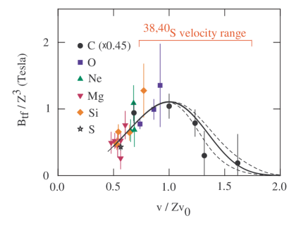
is required to extract the experimental $g$ factors. For light ions ($Z\leq 16$) traversing iron and gadolinium hosts at high velocity, the dependence of the TF strength on the ion velocity, $v$, and atomic number, $Z$, can be parametrized Stuchbery (2004); Stuchbery et al. (2005) as

$$B_{\rm tf}(v,Z)=AZ^{P}(v/Zv_{0})^{2}{\rm e}^{-\frac{1}{2}(v/Zv_{0})^{4}},$$ (14)

where $v_{0}=c/137$ is the Bohr velocity. This is a model-based parametrization that takes account of the known physics of the transient field (see Speidel et al. (2002); Stuchbery (2004); Stuchbery et al. (2005) and references therein). A fit to data for iron hosts yielded $A=1.82(5)$ T with $P=3$ Stuchbery (2004). The experimental data and the adopted parametrization are shown in Fig. 12. The velocity range sampled in the present experiments is also indicated. Although the data are sparse in the high velocity region, there can be no dispute about the general trend, and that the maximum TF strength is reached when the ion velocity matches the $K$-shell electron velocity, $v=Zv_{0}$. Also shown in Fig. 12 are two alternative parametrizations of the field strength in the region $v>Zv_{0}$ chosen to give an indication of the uncertainty in the transient-field calibration. Compared with the adopted parametrization, these extrapolations give values of $\Delta\Theta/g$ that differ by $\sim\pm 12\%$.

Calculations of $\Delta\Theta/g$ were performed using the code GKINT to take into account the incoming and exiting ion velocities, the energy- and angle-dependent Coulomb excitation cross sections in both target layers, the excited-state lifetimes, and the parametrization of the TF strength in Eq. (14). The results and the $g$ factors extracted are given in Table 4.

Figure 12: (Color online) Transient field parametrization (solid line) for high-velocity light ions, from Ref. Stuchbery (2004). Data points are measured transient-field strengths reported in the literature. See  Speidel et al. (2002); Stuchbery (2004); Stuchbery et al. (2005) for further details and references.

The $g$ factor results are not very sensitive to the somewhat uncertain behavior of the transient field at the highest velocities because (i) the ions spend least time interacting with the TF at high velocity and (ii) the TF strength near $2Zv_{0}$ is very small. Furthermore, the positive $g$ factor in ³⁸S and the essentially null effect for ⁴⁰S are both firm observations, independent of the transient-field strength. The $g$ factor of ³⁸S is almost 3 standard deviations from zero.

The experimental uncertainties assigned to the $g$ factors are dominated by the statistical errors in the $\gamma$-ray count ratios, with small contributions from the angular correlation (10%) and transient field calibration (12%) added in quadrature.

Table 4: Experimental results. The spin precession per unit $g$ factor, $(\Delta\Theta/g)_{\rm calc}$, is evaluated for ions that decay after leaving the target. The experimental $g$ factor is given by $g=\Delta\Theta_{\rm exp}/(\Delta\Theta/g)_{\rm calc}$.

Isotope	$(\Delta\Theta/g)_{\rm calc}$	$\Delta\Theta_{\rm exp}$	$g$
	(mrad)	(mrad)
38S	$-330(41)$	$-43(15)$	$+0.13(5)$
40S	$-339(42)$	$+5(21)$	$-0.01(6)$

III.4 Monte Carlo simulations

In the analysis of the data presented above an analytical formalism has been used to evaluate the average angular correlation coefficients, the transient-field precession per unit $g$ factor, and other quantities of interest.

To obtain a more detailed insight into the experiment and data analysis procedures it is helpful to use a Monte Carlo approach to model the experiment. The code GKINT_MCDBLS was written to generate event data for particle-gamma coincidences that can be sorted and correlated with calculated quantities such as the transient-field precession. The effect of the energy spread on the incident beam on the particle spectrum beyond the target was discussed above, and examples of the calculated Doppler broadened $\gamma$-ray line shapes were presented in Fig. 9. Here we examine the behavior of the precession angle and the angular correlation coefficients $a_{2}$ and $a_{4}$ as a function of the detected $\gamma$-ray energy.

Aside from the statistical uncertainties, which can be minimized by increasing the number of events in the simulation, the Monte Carlo approach allows for a rigorous treatment of the decay-in-flight and vacuum deorientation effects. It also properly includes the contributions to the $\gamma$-ray peak that is analyzed to extract the $g$ factor, stemming from excitation in the Au and Fe layers of the target, and which cannot be separated experimentally.

Figure 13: (Color online) Monte Carlo simulations (10⁶ events). Lower panel: Doppler broadened $\gamma$-ray line shape at 29^∘ in the laboratory frame. An equivalent spectrum in the projectile frame is shown in the uppermost panel of Fig. 9. Much of the energy width in the laboratory frame stems from the spread in the projectile velocity, which must be Doppler-corrected event-by-event using the energy from the phoswich detector (section III.1). Middle panel: The transient-field precession per unit $g$ factor as a function of the emitted $\gamma$-ray energy. Upper panel: Angular correlation coefficients as a function of the emitted $\gamma$-ray energy. The effect of vacuum deorientation is indicated by the (red) line labeled $a_{k}G_{k}$.

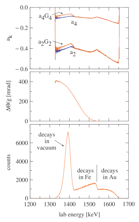
Figure 13 shows how the angular correlation coefficients, $a_{2}$ and $a_{4}$, and the transient field precession, $\Delta\Theta/g$, vary as a function of the $\gamma$-ray line shape in the laboratory frame. A detector at 29^∘ in the laboratory frame was chosen for this comparison. The bump in the line shape near 1540 keV (lower panel) is due to the change in stopping powers as the ³⁸S ions pass into the Fe layer. As can be seen in the middle panel, there is no transient-field precession in the highest part of the Doppler tail (above the bump). This part of the line shape corresponds to ³⁸S ions that are excited and then decay in the Au layer of the target, before reaching the iron layer. As the sulfur ions slow and decay within the iron layer the transient-field precession $\Delta\Theta/g$ increases, reaching its maximum values for those ions that do not decay until they leave the iron layer and emerge into vacuum. The upper part of Fig. 13 shows the variation of both $a_{k}$ and $a_{k}G_{k}$, where $G_{k}$ is the vacuum deorientation coefficient. Clearly, the vacuum deorientation effect applies only to those ions that decay in vacuum, and hence has an effect only in the peak part of the line shape. Aside from the vacuum deorientation effect, the variation in the magnitude of the $a_{k}$ coefficients as a function of the Doppler shift has its origin in the alignment produced by intermediate energy Coulomb excitation Bertulani et al. (2003); Stuchbery (2005). There is a pronounced dependence on the beam energy, such that the alignment is reduced for those projectiles that are excited after losing energy within the target.

At present the variation of the $\gamma$-ray intensity across the acceptance of the detector is not included, and the response of the segmented Ge detector is treated approximately. For example, it is assumed that the hit is always assigned to the correct segment. These approximations are not significant in the present context.

Because the ³⁸S nuclei can be excited in either the Au or Fe layers of the target, and many of them decay before they leave the target and emerge into vacuum, the analytic (GKINT) calculations of $a_{2}G_{2}$, $a_{4}G_{4}$ and $\Delta\Theta/g$ for the vacuum flight peak required some simplifying approximations (mainly to estimate the relative contributions of excitation in the two target layers). The Monte Carlo (GKINT_MCDBLS) calculations, however, enable a simple and rigorous evaluation of these quantities of interest. The disadvantage is that the Monte Carlo calculation is very time consuming. It was found that the difference between the two approaches was small in our case. As well as providing a deeper insight into the experiment, the Monte Carlo calculations therefore support our use of the approximate analytic calculations, which introduce negligible error compared with the statistical uncertainties in the experiment.

IV Shell model and discussion

IV.1 Shell model calculations

Shell model calculations were performed for ${}^{36}_{16}$S₂₀, ${}^{38}_{16}$S₂₂ and ${}^{40}_{16}$S₂₄, and their isotones ${}^{38}_{18}$Ar₂₀, ${}^{40}_{18}$Ar₂₂ and ${}^{42}_{18}$Ar₂₄, using the code OXBASH Brown et al. (2004) and the $sd$-$pf$ model space where (for $N\geq 20$) valence protons are restricted to the $sd$ shell and valence neutrons are restricted to the $pf$ shell. The Hamiltonian was that developed in Ref. Nummela et al. (2001) for neutron-rich nuclei around $N=28$, i.e. the SDPF-NR interaction Caurier et al. (2005). These calculations reproduce the energies of the low-excitation states to within 200 keV. With standard effective charges of $e_{p}\sim 1.5$ and $e_{n}\sim 0.5$ they also reproduce the measured $B(E2)$ values. The relevant results for the 2${}^{+}_{1}$ states are summarized in Table 5, where they are labeled SDPF. For the purposes of the following discussion, the $B(E2)$ and $Q(2^{+})$ values are also presented in terms of the equivalent deformation parameter $\beta$. These electric quadrupole properties have been calculated and discussed by Retamosa et al. Retamosa et al. (1997). Although the shell model Hamiltonian has been improved since their work, the theoretical $B(E2)$ and deformation values agree closely with the values in Table 5, and their discussion remains relevant.

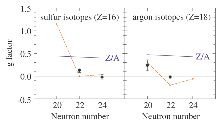
The $g$ factors of the 2${}^{+}_{1}$ states were evaluated using the bare nucleon $g$ factors. The calculated $g$ factors are compared with experimental results in Fig. 14 and Table 6, which also shows the orbital and spin contributions to the $g$ factor originating from both protons and neutrons. As will be discussed below, the overall level of agreement between theory and experiment is satisfactory given the extreme sensitivity to configuration mixing and the near cancelation of proton and neutron contributions in the $N=22,24$ isotones.

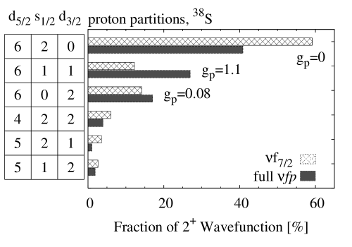
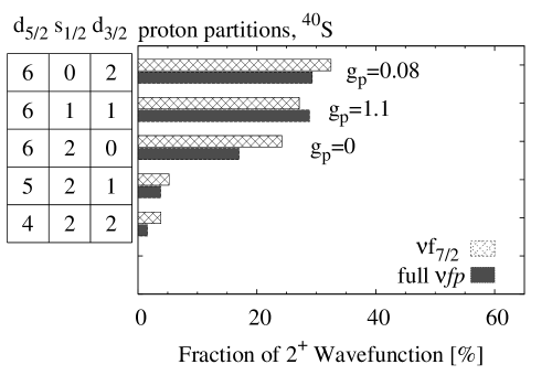
The main partitions of the 2${}^{+}_{1}$-state wavefunctions in ³⁸S and ⁴⁰S are indicated in Table 7. Table 8 shows the decomposition of the $g(2^{+})$ values into the contributions from each combination of single-particle orbitals for ^38,40S and ^38,40Ar. The off-diagonal contributions from spin-orbit partner orbits can play an important role. In ³⁸S and ⁴⁰S they tend to quench the (diagonal) moment of the dominant configuration.

Many authors have argued on experimental and theoretical grounds that ⁴⁰S ($N=24$) is deformed, some linking it to a weakening of the $N=28$ shell gap (see Refs. Scheit et al. (1996); Glasmacher et al. (1997); Winger et al. (2001); Sohler et al. (2002); Rodríguez-Guzmán et al. (2002); Caurier et al. (2004); Retamosa et al. (1997) and references therein). To explore the role of excitations across the $N=28$ shell gap, a further set of calculations was performed in which the neutrons were confined to the $f_{7/2}$ orbit. The results of these calculations, labeled SDF, are given in Tables 5 and 6.

Table 5: Theoretical and experimental excitation energies, quadrupole moments, and $B(E2)$ values. Experimental data are from Raman et al. (2001).

Nuclide	Model	$E_{2^{+}}^{\rm th}$	$E_{2^{+}}^{\rm exp}$	$Q(2^{+}_{1})$	$B(E2)\uparrow^{\rm th}$	$B(E2)\uparrow^{\rm exp}$	$\beta^{\rm th}_{Q}$	$|\beta^{\rm th}_{E2}|$	$|\beta^{\rm exp}_{E2}|$
		(MeV)	(MeV)	($e$ fm2)	($e^{2}$ fm4)	($e^{2}$ fm4)
36S	SDPF	3.426	3.291	$-11.6$	141	104(28)	$+0.21$	0.20	0.17(2)
38S	SDPF	1.531	1.292	$-9.7$	268	235(30)	$+0.17$	0.26	0.25(2)
	SDF	1.286		$+7.5$	158		$-0.13$	0.20
40S	SDPF	0.980	0.904	$-19.3$	473	334(36)	$+0.33$	0.34	0.28(2)
	SDF	1.052		$-9.8$	328		$+0.17$	0.28
38Ar	SDPF	2.018	2.167	$+4.3$	178	130(10)	$-0.07$	0.19	0.16(1)
40Ar	SDPF	1.371	1.461	$+8.5$	263	330(40)	$-0.13$	0.22	0.25(2)
	SDF	0.966		$+12.8$	228		$-0.20$	0.21
42Ar	SDPF	1.243	1.208	$+5.2$	360	430(10)	$-0.08$	0.25	0.28(3)
	SDF	0.918		$+13.5$	317		$-0.20$	0.24

Table 6: Theoretical $g$ factors compared with experiment.

Nuclide	Model	$g^{\rm th}_{\rm proton}$			$g^{\rm th}_{\rm neutron}$	$g^{\rm th}$	$g^{\rm exp}$
		orbital	spin	total
${}^{36}_{16}$S20	SDPF	0.967	0.187	$+1.154$	0	$+1.154$
${}^{38}_{16}$S22	SDPF	0.225	0.073	$+0.298$	$-0.301$	$-0.003$	$+0.13(5)$
	SDF	0.087	0.049	$+0.136$	$-0.494$	$-0.358$
${}^{40}_{16}$S24	SDPF	0.225	0.051	$+0.276$	$-0.241$	$+0.035$	$-0.01(6)$
	SDF	0.249	0.070	$+0.318$	$-0.404$	$-0.085$
${}^{38}_{18}$Ar20	SDPF	1.151	$-0.842$	$+0.308$	0	$+0.308$	$+0.24(12)$
${}^{40}_{18}$Ar22	SDPF	0.311	$-0.147$	$+0.164$	$-0.364$	$-0.200$	$-0.02(4)$
	SDF	0.228	$-0.092$	$+0.136$	$-0.431$	$-0.295$
${}^{42}_{18}$Ar24	SDPF	0.263	$-0.043$	$+0.220$	$-0.280$	$-0.060$
	SDF	0.242	$-0.025$	$+0.217$	$-0.417$	$-0.200$

Table 7: Partitions $>5\%$ contributing to the wavefunctions of the $2_{1}^{+}$ states of ³⁸S and ⁴⁰S in the SDPF model.

nuclide	proton orbit			neutron orbit				occupation (%)
	$1d_{5/2}$	$1d_{3/2}$	$2s_{1/2}$	$1f_{7/2}$	$1f_{5/2}$	$2p_{3/2}$	$2p_{1/2}$
38S	6	0	2	2	0	0	0	26.89
	6	1	1	2	0	0	0	18.36
	6	2	0	2	0	0	0	12.10
	6	0	2	1	0	1	0	12.01
	6	1	1	1	0	1	0	6.36
40S	6	2	0	4	0	0	0	17.26
	6	1	1	4	0	0	0	16.22
	6	0	2	4	0	0	0	9.30
	6	2	0	3	0	1	0	9.18
	6	1	1	3	0	1	0	8.37
	6	0	2	3	0	1	0	6.05

Table 8: Contributions to the $g$ factors of the $2_{1}^{+}$ states in ³⁸S, ⁴⁰S, ³⁸Ar and ⁴⁰Ar for the SDPF model.

orbits	38S	40S	38Ar	40Ar
$\pi$ $1d_{5/2}$ - $1d_{5/2}$	0.046	0.067	0.044	0.033
$\pi$ $1d_{5/2}$ - $1d_{3/2}$	$-0.015$	$-0.003$	0.124	0.003
$\pi$ $1d_{3/2}$ - $1d_{3/2}$	0.014	0.014	0.080	0.021
$\pi$ $2s_{1/2}$ - $2s_{1/2}$	0.254	0.199	0.061	0.107
$\nu$ $1f_{7/2}$ - $1f_{7/2}$	$-0.430$	$-0.447$		$-0.394$
$\nu$ $1f_{7/2}$ - $1f_{5/2}$	0.039	0.118		$-0.002$
$\nu$ $1f_{5/2}$ - $1f_{5/2}$	0.009	0.011		0.005
$\nu$ $2p_{3/2}$ - $2p_{3/2}$	0.054	0.092		0.018
$\nu$ $2p_{3/2}$ - $2p_{1/2}$	0.026	$-0.016$		0.008
$\nu$ $2p_{1/2}$ - $2p_{1/2}$	0.002	0.000		0.001

Figure 14: (Color online) Theoretical $g$ factors compared with experiment. The dashed line shows the present shell model calculations. The previous results for ³⁸Ar and ⁴⁰Ar are from Refs. Speidel et al. (2006) and Stefanova et al. (2005), respectively.

IV.2 Discussion of results

In the $N=20$ isotones, ³⁶S and ³⁸Ar, the 2${}^{+}_{1}$ state is a pure proton excitation for our model space. In ³⁶S the first-excited state at 3.29 MeV is dominated (87%) by the proton $(s_{1/2}d_{3/2})_{2^{+}}$ configuration for which $g=+1.459$. The 2${}^{+}_{1}$ configuration in ³⁸Ar is predominantly (93%) $\pi(d_{3/2})^{2}_{2^{+}}$ for which $g=+0.083$. This case demonstrates the extreme sensitivity of the magnetic moments to configuration mixing - the remaining 7% of the wavefunction raises the calculated moment to $+0.308$, in agreement with the experimental value Speidel et al. (2006). It also shows the importance of off-diagonal terms (see Table 8) as the diagonal contributions associated with the two main configurations account for only 60% of the total theoretical $g$ factor.

Two neutrons have been added to the $pf$ shell in the $N=22$ isotones ³⁸S and ⁴⁰Ar. Since ³⁶S is almost doubly magic, the initial expectation might be that the first-excited state of ³⁸S would be dominated by the neutron $f_{7/2}$ configuration weakly coupled to the ³⁶S core, resulting in a $g$ factor near $-0.3$. An example of this type of behavior is the $N=52$ isotope ${}^{92}_{40}$Zr₅₂ Jakob et al. (1999); Stuchbery et al. (2004); the effect is also evident, but less pronounced, in ${}^{94}_{42}$Mo₅₂ Mantica et al. (2001). In contrast with this weak-coupling scenario, the near zero theoretical $g$ factor and the small but positive experimental $g$ factor of ³⁸S require additional proton excitations, which indicate strong coupling between protons and neutrons. It is relevant to note that strong proton-neutron coupling is considered one of the prerequisites for the onset of deformation. The effect on the proton configuration due to coupling with neutrons in orbits above the $N=28$ shell gap will be discussed below.

For $N=22,24$ the shell model predicts a cancelation of the proton and neutron contributions to the moment. Under these conditions, the description of the $g$ factors is satisfactory. The dependence of the $g(2^{+})$ in ⁴⁰Ar on the basis space, the interaction, and the choice of effective nucleon $g$ factors, has been investigated in Ref. Stefanova et al. (2005). To estimate the impact of the use of effective $g$ factors, we recalculated the $g(2^{+})$ values in Table 6 adopting the effective $g_{l}$ and $g_{s}$ values employed by Stefanova et al. The effect was to make the $2^{+}$-state $g$ factors more positive, by $\sim 0.05$ for the S isotopes and by $\sim 0.1$ for the Ar isotopes; the discrepancy between theory and experiment for ³⁸S and ⁴⁰Ar is therefore reduced, but not eliminated by the use of effective $g$ factors.

A comparison may also be made between ³⁸S and ⁴⁰S, and their isotones ⁴²Ca and ⁴⁴Ca, where the experimental $g$ factors, $g(2^{+})=+0.04(6)$ and $g(2^{+})=+0.16(3)$, are also far from that of the $\nu f_{7/2}^{2}$ configuration Schielke et al. (2003); Taylor et al. (2003). In both ⁴²Ca and ⁴⁴Ca there is evidently a significant collective component in the wavefunction that cannot readily be included in shell model calculations Schielke et al. (2003); Taylor et al. (2003). Some remnant of this collective excitation may occur in ³⁸S and ⁴⁰S, although it is very much smaller than in the calcium isotopes.

We conclude that the dominant components of the shell model wavefunctions are correct and give a satisfactory description of the measured $g$ factors. As such, the shell model calculations provide a microscopic explanation of the development of quadrupole collectivity in these nuclei, which will now be discussed in more detail.

The existence of deformation in nuclei has long been associated with strong interactions between a significant number of valence protons and neutrons, particularly in nuclei near the middle of a major shell. Without exception the deformed nuclei studied to date have $g$ factors near the hydrodynamical limit, $Z/A$, reflecting the strong coupling between protons and neutrons, and a magnetic moment dominated by the orbital motion of the proton charge with small contributions from the intrinsic magnetic moments of either the protons or the neutrons. Examples include ²⁴Mg in the $sd$ shell Brown (1982), and ⁵⁰Cr in the $pf$ shell Ernst et al. (2000). Robinson et al. Robinson et al. (2006) have recently used the shell model to examine the relation between the $B(E2)$, $Q(2^{+}_{1})$ and the orbital magnetic dipole strength (scissors mode) in these nuclei.

As noted above, Coulomb-excitation studies and the level scheme of ⁴⁰S suggest that it is deformed. Supporting this interpretation, the shell model calculations (Table 5) predict consistent intrinsic quadrupole moments when derived from either the $B(E2)$ or the quadrupole moment, $Q(2^{+}_{1})$, implying a prolate deformation of $\beta\approx+0.3$, in agreement with the value deduced from the experimental $B(E2)$ Scheit et al. (1996). The near zero magnetic moment, however, does not conform to the usual collective model expectation of $g\sim Z/A$. Since the shell model calculations reproduce both the electric and magnetic properties of the 2${}^{+}_{1}$ state they give insight into the reasons for this unprecedented magnetic behavior in an apparently deformed nucleus.

The essential difference between the deformed neutron-rich sulfur isotopes and the deformed nuclei previously encountered (i.e. either light nuclei with $N=Z$ or heavier deformed nuclei) is that the spin contributions to the magnetic moments are relatively more important, especially for the neutrons. It can be seen from Table 6 that the proton contributions to the $g$ factors are dominated by the orbital component, as is usually the case for deformed nuclei, but the substantial neutron contributions originate entirely with the intrinsic spin. The main partitions of the shell-model wavefunctions summarized in Table 7 indicate that both ³⁸S and ⁴⁰S have a dominant occupation of the neutron $f_{7/2}$ orbit, for which $g=-0.547$ (unless coupled to spin zero). The net neutron contribution to the $g$ factor in ³⁸S (⁴⁰S) is therefore $\sim 55\%$ ($\sim 44\%$) of that of a pure $f_{7/2}$ neutron configuration. Those configurations with neutron excitations into the $p_{3/2}f_{5/2}p_{1/2}$ shell mainly have a single occupation of the $p_{3/2}$ orbit. Although these excitations tend to reduce the magnetic moment of the neutrons from the value of the pure $f_{7/2}^{n}$ configuration, they do not cancel the neutron magnetic moment altogether because the $g$ factor of the $\nu(f_{7/2}\otimes p_{3/2})_{J}$ configuration coupled to spin $J=2$ is $-0.183$, and the value increases in magnitude for other possible values of $J$. The off-diagonal terms in the $M1$ operator also quench the $f_{7/2}$ neutron contribution to $g(2^{+})$, as indicated in Table 8.

Figure 15: Dominant proton partitions in ³⁸S comparing calculations in which neutrons occupy the full $pf$ shell (SDPF) with calculations in which they are restricted to the $f_{7/2}$ shell (SDF). The $g$ factors which represent the diagonal contributions of the most important configurations are indicated.

Figure 16: As for Fig. 15, but for ⁴⁰S.

The role of neutron excitations across the $N=28$ shell gap can be examined further by comparing the calculations using the full SDPF model space with the truncated SDF calculations in which the neutrons were restricted to the $f_{7/2}$ shell. Looking first at the $E2$ properties presented in Table 5, it is apparent from the $Q(2^{+})$ values that excitations into the $p_{3/2}f_{5/2}p_{1/2}$ shell are needed to produce significant prolate deformations in ³⁸S and ⁴⁰S. Furthermore, in ⁴⁰S, the quadrupole moment and $B(E2)$ are not consistent with the same intrinsic quadrupole deformation unless the neutrons can occupy the $p_{3/2}f_{5/2}p_{1/2}$ shell. The wavefunctions in Table 7 indicate that the development of quadrupole collectivity depends most sensitively upon the occupation of the $\nu p_{3/2}$ orbit.

Turning to the $g$ factors, it is apparent that two effects are important. First, in all cases the neutron contribution to $g(2^{+})$ is quenched significantly when the $p_{3/2}f_{5/2}p_{1/2}$ orbits are occupied. Second, the case of ³⁸S shows a dramatic change in the $g$ factor due to a relatively small neutron occupation of the $p_{3/2}$ orbit, highlighting that there is a strong coupling between the protons and neutrons. Specifically, a small occupation of the neutron $p_{3/2}$ orbit, moves the theoretical $g$ factor from $-0.358$ to $-0.003$, falling short of the experimental value by a small margin compared with the distance traveled. Fig. 15 shows how the proton partition of the wavefunction for ³⁸S changes significantly with the occupation of the $p_{3/2}f_{5/2}p_{1/2}$ shell; there is a significant increase in the contribution of the proton $s_{1/2}d_{3/2}$ configuration, which has a large $g$ factor, and which has been proposed to drive deformation. In contrast, Fig. 16 shows that for ⁴⁰S this proton configuration contributes strongly to the wavefunction whether excitations across the $N=28$ gap are allowed or not. Apparently the effect of a single neutron occupying the $p_{3/2}$ orbit is diluted when three remain in the $f_{7/2}$ shell.

Since the hydrodynamical collective models fail to explain the $g$ factor of ⁴⁰S, the observed quadrupole collectivity in this region is better interpreted in terms of the symmetries of the shell model Hamiltonian. More specifically, the development of quadrupole collectivity can be linked to the quasi-$SU(3)$ symmetry identified by Zuker et al. Zuker et al. (1995) and considered for the sulfur isotopes by Retamosa et al. Retamosa et al. (1997). In the neutron space the $\Delta j=2$ orbits $f_{7/2}$-$p_{3/2}$ develop the quasi-$SU(3)$ symmetry. As shown by the comparisons in Table 5, occupation of the $p_{3/2}$ orbit is clearly essential if quadrupole collectivity is to emerge. Turning to the proton space, for the S isotopes of interest the proton $d_{5/2}$ orbit is essentially closed and only the $d_{3/2}$ and $s_{1/2}$ orbits are active (see Table 7). Although quasi-$SU(3)$ cannot develop for these two orbits, an approximate pseudo-$SU(3)$ geometry does develop. When neutrons begin to fill the $pf$ shell, the effective energies of the two proton orbits become increasingly degenerate, as is manifested by the narrowing of the gap between the lowest $3/2^{+}$ and $1/2^{+}$ states in the odd-$A$ isotopes of K, Cl and P Cottle and Kemper (1998); Fridmann et al. (2005). In the limit of degenerate $d_{3/2}$ and $s_{1/2}$ orbits the valence proton space has the geometry of pseudo-$SU(3)$. Within this framework, quadrupole collectivity develops in the neutron-rich sulfur isotopes because the proton number is optimal for quadrupole coherence, despite the fact that the $d_{3/2}$ - $s_{1/2}$ degeneracy is not reached Retamosa et al. (1997).

The shift in the effective single particle energies of the proton $d_{3/2}$ and $s_{1/2}$ orbits is strongly linked to the effect of the monopole component of the tensor term in the nucleon-nucleon interaction. Otsuka et al. Otsuka et al. (2005) have shown that the effect of the monopole interaction between the proton $d_{3/2}$ and neutron $f_{7/2}$ orbits is attractive, which narrows the gap between the proton $d_{3/2}$ and $s_{1/2}$ states as more and more neutrons are added to the $f_{7/2}$ shell. This effect of the monopole interaction is therefore more pronounced in ⁴⁰S than in ³⁸S, and may explain why the contribution of the proton partition $d_{5/2}^{6}s_{1/2}^{1}d_{3/2}^{1}$ is less sensitive to the neutron occupation of the $p_{3/2}$ orbit in ⁴⁰S than in ³⁸S.

V Summary and conclusion

In summary, we have developed a high-velocity transient-field technique to measure the $g$ factors of excited states of neutron-rich nuclei produced as fast radioactive beams. The $g$ factors of the first-excited states in the neutron-rich isotopes ³⁸S and ⁴⁰S have been measured with sufficient precision to test and challenge shell model calculations.

Keys to the success of these measurements on low intensity radioactive beams (10⁴ to 10⁵ pps) include (i) the use of intermediate energy Coulomb-excitation to align the nuclear spin, and (ii) exploitation of the high velocities of the fragment beams to maximize the transient-field precession angle. In these measurements the precession angle per unit $g$ factor is $\sim 10$ times that in conventional measurements on neighboring nuclei Speidel et al. (2006); Stefanova et al. (2005); Schielke et al. (2003); Taylor et al. (2003).

The nature and origin of the quadrupole collectivity that develops between $N=20$ and $N=28$, including the role of excitations across the $N=28$ shell gap, has been explored by comparing the measured $g$ factors with shell model calculations.

The case of ³⁸S highlights the role of strong proton-neutron interactions, showing that neutron excitations across the $N=28$ shell gap cause a large change in the proton configuration. Taken together with the results for ⁴⁰S, it seems that excitations across the $N=28$ shell gap and the reduction in the proton $s_{1/2}$-$d_{3/2}$ gap due to increasing neutron occupation of the $f_{7/2}$ orbit both contribute to the development of collectivity.

Since the hydrodynamical collective models fail to explain the $g$ factor of ⁴⁰S, the observed quadrupole collectivity in this region should be interpreted in terms of the symmetries of the shell model Hamiltonian. The unusual combination of magnetic and electric properties in ⁴⁰S apparently comes about because relatively few particles are involved in the collective motion. These features reemphasize the unique mesoscopic nature of the nucleus.

Looking to future applications of the high-velocity transient-field technique, it may be noted that the 2${}^{+}_{1}$ state in the $N=20$ nucleus ${}^{32}_{12}$Mg₂₀ has a similar excitation energy, lifetime and $B(E2)$ to ⁴⁰S. However the $g$ factor in ³²Mg might be closer to that of a conventional collective nucleus since the $N=20$ shell closure is known to vanish far from stability. Indeed a shell model calculation using the interactions of Warburton, Becker and Brown Warburton et al. (1990) gives $g=g_{p}+g_{n}=0.52-0.11=+0.41$, close to the collective value of $Z/A=0.375$.

References

- Davies et al. (2006a) A. D. Davies, A. E. Stuchbery, P. F. Mantica, P. M. Davidson, A. N. Wilson, A. Becerril, B. A. Brown, C. M. Campbell, J. M. Cook, D. C. Dinca, et al., Phys. Rev. Lett. 96, 112503 (2006a).
- Stuchbery (2004) A. E. Stuchbery, Phys. Rev. C 69, 064311 (2004).
- Davies et al. (2006b) A. D. Davies, A. E. Stuchbery, and P. F. Mantica (2006b), to be published.
- Raman et al. (2001) S. Raman, C. W. Nestor, and P. Tikkanen, At. Data Nucl. Data Tables 78, 1 (2001).
- Scheit et al. (1996) H. Scheit, T. Glasmacher, B. A. Brown, J. A. Brown, P. D. Cottle, P. G. Hansen, R. Harkewicz, M. Hellström, R. W. Ibbotson, J. K. Jewell, et al., Phys. Rev. Lett. 77, 3967 (1996).
- Glasmacher et al. (1997) T. Glasmacher, B. A. Brown, M. J. Chromik, P. D. Cottle, M. Fauerbach, R. W. Ibbotson, K. W. Kemper, D. J. Morrissey, H. Scheit, D. W. Sklenicka, et al., Phys. Lett. B 395, 163 (1997).
- Winger et al. (2001) J. A. Winger, P. F. Mantica, R. M. Ronningen, and M. A. Caprio, Phys. Rev. C 64, 064318 (2001).
- Sohler et al. (2002) D. Sohler, Z. Dombrádi, J. Timár, O. Sorlin, F. Azaiez, F. Amorini, M. Belleguic, C. Bourgeois, C. Donzaud, J. Duprat, et al., Phys. Rev. C 66, 054302 (2002).
- Werner et al. (1994) T. R. Werner, J. A. Sheikh, W. Nazarewicz, M. R. Strayer, A. S. Umar, and M. Misu, Phys. Lett. B 335, 259 (1994).
- Cottle and Kemper (1998) P. D. Cottle and K. W. Kemper, Phys. Rev. C 58, 3761 (1998).
- Rodríguez-Guzmán et al. (2002) R. Rodríguez-Guzmán, J. L. Edigo, and L. M. Robledo, Phys. Rev. C 65, 024304 (2002).
- Caurier et al. (2004) E. Caurier, F. Nowacki, and A. Poves, Nucl. Phys. A 742, 14 (2004).
- Glasmacher (1998) T. Glasmacher, Annu. Rev. Nucl. Sci. 48, 1 (1998).
- Benczer-Koller et al. (1980) N. Benczer-Koller, M. Hass, and J. Sak, Annu. Rev. Nucl. Sci. 30, 53 (1980).
- Speidel et al. (2002) K.-H. Speidel, O. Kenn, and F. Nowacki, Prog. Part. Nucl. Phys. 49, 91 (2002).
- Morrissey et al. (2003) D. J. Morrissey, B. M. Sherrill, M. Steiner, A. Stolz, and I. Wiedenhoever, Nucl. Inst. Meth. Phys. Res. B 204, 90 (2003).
- Ziegler et al. (1985) J. F. Ziegler, J. P. Biersack, and U. Littmark, The stopping and range of ions in solids (Permagon, New York, 1985), vol. 1 of The stopping and ranges of ions in matter, ed. J.F. Ziegler.
- Stuchbery et al. (2006) A. E. Stuchbery, A. D. Davies, and P. F. Mantica (2006), to be published.
- Piqué et al. (1989) A. Piqué, J. M. Brennan, R. Darling, R. Tanczyn, D. Ballon, and N. Benczer-Koller, Nucl. Inst. Meth. A 279, 579 (1989).
- Mueller et al. (2001) W. F. Mueller, J. A. Church, T. Glasmacher, D. Gutknecht, G. Hackman, P. G. Hansen, Z. Hu, K. L. Miller, and P. Quirin, Nucl. Inst. Meth. Phys. Res. A 466, 492 (2001).
- Miller et al. (2002) K. L. Miller, T. Glasmacher, C. Campbell, L. Morris, W. F. Mueller, and E. Strahler, Nucl. Inst. Meth. Phys. Res. A 490, 140 (2002).
- Bertulani et al. (2003) C. A. Bertulani, A. E. Stuchbery, T. J. Mertzimekis, and A. D. Davies, Phys. Rev. C 68, 044609 (2003).
- Stuchbery et al. (2006) A. E. Stuchbery, P. M. Davidson, and A. N. Wilson, Nucl. Instr. Meth. Phys. Res. B 243, 265 (2006).
- Goldring (1982) G. Goldring, in Heavy Ion Collisions, edited by R. Bock (North-Holland, Amsterdam, 1982), vol. 3, p. 484.
- Stuchbery (2005) A. E. Stuchbery, Some notes on the program GKINT: Transient-field -factor kinematics at intermediate energies, Department of Nuclear Physics, The Australian National University, report no. ANU-P/1678 (2005).
- Stuchbery (2003) A. E. Stuchbery, Nucl. Phys. A 723, 69 (2003).
- Olliver et al. (2003) H. Olliver, T. Glasmacher, and A. E. Stuchbery, Phys. Rev. C 68, 044312 (2003).
- Jakob et al. (1999) G. Jakob, N. Benczer-Koller, J. Holden, G. Kumbartzki, T. J. Mertzimekis, K.-H. Speidel, C. W. Beausang, and R. Krücken, Phys. Lett. B 468, 13 (1999).
- Mantica et al. (2001) P. F. Mantica, A. E. Stuchbery, D. E. Groh, J. I. Prisciandaro, and M. P. Robinson, Phys. Rev. C 63, 034312 (2001).
- Stuchbery et al. (2005) A. E. Stuchbery, A. N. Wilson, P. M. Davidson, A. D. Davies, T. J. Mertzimekis, S. N. Liddick, B. E. Tomlin, and P. F. Mantica, Phys. Lett. B 611, 81 (2005).
- Brown et al. (2004) B. A. Brown, A. Etchegoyen, N. S. Godwin, W. D. M. Rae, W. A. Richter, W. E. Ormand, E. K. Warburton, J. S. Winfield, L. Zhao, and C. H. Zimmerman, Oxbash for Windows PC, Michigan State University, report no. MSU-NSCL 1289 (2004).
- Nummela et al. (2001) S. Nummela, P. Baumann, E. Caurier, P. Dessagne, A. Jokinen, A. Knipper, G. Le Scornet, C. Miehé, F. Nowacki, M. Oinonen, et al., Phys. Rev. C 63, 044316 (2001).
- Caurier et al. (2005) E. Caurier, G. Martinez-Pinedo, F. Nowacki, A. Poves, and A. P. Zuker, Reviews of Modern Physics 77, 427 (2005).
- Retamosa et al. (1997) J. Retamosa, E. Caurier, F. Nowacki, and A. Poves, Phys. Rev. C 55, 1266 (1997).
- Speidel et al. (2006) K.-H. Speidel, S. Schielke, J. Leske, J. Gerber, P. Maier-Kormor, S. J. Q. Robinson, Y. Y. Sharon, and L. Zamick, Phys. Lett. B 632, 207 (2006).
- Stefanova et al. (2005) E. A. Stefanova, N. Benczer-Koller, G. J. Kumbartzki, Y. Y. Sharon, L. Zamick, S. J. Q. Robinson, L. Bernstein, J. R. Cooper, D. Judson, M. J. Taylor, et al., Phys. Rev. C 72, 014309 (2005).
- Stuchbery et al. (2004) A. E. Stuchbery, N. Benczer-Koller, G. Kumbartzki, and T. J. Mertzimekis, Phys. Rev. C 69, 044302 (2004).
- Schielke et al. (2003) S. Schielke, D. Hohn, K.-H. Speidel, O. Kenn, J. Leske, N. Gemein, M. Offer, J. Gerber, P. Maier-Komor, O. Zell, et al., Phys. Lett. B 571, 29 (2003).
- Taylor et al. (2003) M. J. Taylor, N. Benczer-Koller, G. Kumbartzki, T. J. Mertzimekis, S. J. Q. Robinson, Y. Y. Sharon, L. Zamick, A. E. Stuchbery, C. Hutter, C. W. Beausang, et al., Phys. Lett. B 559, 187 (2003).
- Brown (1982) B. A. Brown, J. Phys. G: Nucl. Phys. 8, 679 (1982).
- Ernst et al. (2000) R. Ernst, K.-H. Speidel, O. Kenn, A. Gohla, U. Nachum, J. Gerber, P. Maier-Komor, N. Benczer-Koller, G. Kumbartzki, G. Jakob, et al., Phys. Rev. C 62, 024305 (2000).
- Robinson et al. (2006) S. J. Q. Robinson, A. Escuderos, L. Zamick, P. von Neumann-Cosel, A. Richter, and R. W. Fearick, Phys. Rev. C 73, 037306 (2006).
- Zuker et al. (1995) A. P. Zuker, J. Retamosa, A. Poves, and E. Caurier, Phys. Rev. C 52, R1741 (1995).
- Fridmann et al. (2005) J. Fridmann, I. Wiedenhöver, A. Gade, L. T. Baby, B. D., B. A. et al Brown, C. M. Campbell, J. M. Cook, P. D. Cottle, E. Diffenderfer, et al., Nature 435, 922 (2005).
- Otsuka et al. (2005) T. Otsuka, T. Suzuki, R. Fujimoto, H. Grawe, and Y. Akaishi, Phys. Rev. Lett. 95, 232502 (2005).
- Warburton et al. (1990) E. K. Warburton, J. A. Becker, and B. A. Brown, Phys. Rev. C 41, 1147 (1990).