Perturbed angular correlations for Gd in gadolinium: in-beam comparisons of relative magnetizations

Abstract

Perturbed angular correlations were measured for Gd ions implanted into gadolinium foils following Coulomb excitation with 40 MeV ¹⁶O beams. A technique for measuring the relative magnetizations of ferromagnetic gadolinium hosts under in-beam conditions is described and discussed. The combined electric-quadrupole and magnetic-dipole interaction is evaluated. The effect of nuclei implanted onto damaged or non-substitutional sites is assessed, as is the effect of misalignment between the internal hyperfine field and the external polarizing field. Thermal effects due to beam heating are discussed.

, , ,

1 Introduction

Gadolinium foils are used extensively for in-beam measurements of hyperfine interactions and nuclear moments [1, 2, 3, 4, 5, 6, 7, 8, 9, 10, 11, 12, 13]. Magnetized gadolinium foils are used in preference to iron foils in many applications of the transient-field technique [5, 13] to measure nuclear $g$ factors because larger perturbations of the particle-$\gamma$ correlations can be obtained under otherwise similar experimental conditions [6, 7]. One disadvantage of gadolinium hosts, however, is that the magnetization is not well controlled, being sensitive to the crystalline structure of the foil, and varying considerably with both the applied field and the temperature, even at temperatures well below the Curie temperature of 293 K [14].

As cooling with liquid nitrogen (77 K) is convenient in accelerator laboratories, most in-beam measurements which employ gadolinium hosts have been performed at somewhat higher temperatures near 90 K because of thermal losses and the effects of beam heating on the target. In transient-field measurements an external magnetic field, with strength typically in the range from 0.05 to 0.1 T, is applied to polarize the gadolinium foil. Higher fields are avoided to ensure that bending of the primary beam is negligible [15, 13]. The spacial profile of the polarizing field along the beam direction is designed to minimize beam bending effects rather than to produce a uniform field at the target location. Depending upon the design of the pole pieces and the location of the target, the profile of the external field across the target may not be uniform. Under these conditions the magnetization in the beam spot must be carefully related to the off-line magnetization measurements.

In this paper a method of determining the relative magnetization of gadolinium foils under in-beam conditions is described. The static hyperfine magnetic field, which acts on the nuclei of Coulomb excited 2${}^{+}_{1}$ states in ^{154,156,158,160}Gd, is used to probe the local magnetization at the beam spot under in-beam conditions.

Measurements similar to the present work were performed by Skaali et al. [1], and Kalish et al. [3]. Additional complementary information was also obtained by Häusser et al. [6]. In these previous works, however, the focus was on the precessions of the 4${}^{+}_{1}$ and 6${}^{+}_{1}$ states as probes of the strength of the transient hyperfine magnetic field. Here the emphasis is on the 2${}^{+}_{1}$ states and the strength of the static hyperfine magnetic field.

While the interpretation of the hyperfine interactions in terms of the relative magnetization of different samples turns out to be rather straight-forward, there are several additional phenomena associated with the hyperfine fields and the ion-implantation process that may have bearing on the interpretation of the data. The present work will therefore include discussions of:

1. the presence of the electric-field gradient in the gadolinium matrix, which means that the hyperfine interaction cannot universally be treated as a pure magnetic interaction

2. the effects of those implanted nuclei which reside on damaged or other non-substitutional sites

3. the magnitude of the transient hyperfine magnetic field, which acts on the implanted ions as they slow within the host, and which for Gd in gadolinium has the opposite sign to the static hyperfine field

4. a possible misalignment between the hyperfine magnetic field and the external polarizing field, which can affect the interpretation of the perturbed angular correlation when the host is not fully saturated

The paper is arranged as follows: The next section (section 2) reviews previous work on the electric and magnetic hyperfine fields experienced by Gd ions in gadolinium. Section 3 describes the in-beam measurements, presents examples of $\gamma$-ray and particle spectra, and summarizes the excited-state lifetimes, $g$ factors and quadrupole moments adopted for the analysis. The off-line magnetization measurements are presented in section 4. Section 5 concerns the ‘unperturbed’ angular correlations measured at room temperature. It includes a review of the formalism, along with the results and a discussion of the measurements, which indicate the direction of the electric-field gradient in the gadolinium foils. The perturbed angular correlation results are presented in section 6. The formalism and data analysis procedures are described, the effects of combined electric-quadrupole and magnetic-dipole interactions are evaluated, as are the effects of nuclei on damaged sites. The results are discussed in Section 7.

2 Hyperfine fields in gadolinium hosts

Gadolinium has a hexagonal close packed (hcp) crystal structure. Nuclei within the gadolinium matrix therefore experience a hyperfine electric-field gradient along with the magnetic dipole interaction. Below the Curie temperature of 293 K, gadolinium is a simple ferromagnet with a magnetic anisotropy that has a complex dependence on temperature. Thus the easy direction of magnetization changes as a function of temperature, as does the magnetic hyperfine field. Mössbauer studies [2] reveal anisotropic magnetic hyperfine interactions in gadolinium crystals, with a field of $|B_{\rm st}|=37.3(5)$ T at 4.2 K oriented at 28^∘ to the $c$ axis (unpolarized sample). The electric field gradient is apparently less sensitive to temperature [8]. The measured splitting at 4.2 K for ¹⁵⁵Gd, $eqQ/h=108\pm 1$ MHz, implies an electric field gradient of $V_{zz}=3.44(6)\times 10^{17}$ V/cm², assuming $Q=1.30(2)$ b. This electric field gradient is consistent with that found for high-spin isomers in ^147,148Gd at temperatures near 400 K [8].

The electric-quadrupole and magnetic-dipole hyperfine fields acting on Gd isotopes in various gadolinium samples at different temperatures have been studied previously by many techniques (see Refs. [2, 4, 8] and references therein). In the present work the Mössbauer values at 4.2 K will be taken as the point of reference. The sign of the static magnetic field has been determined to be negative, for example from in-beam perturbed angular correlation measurements [1, 3, 6].

Since the present work concerns in-beam implantation of Gd into gadolinium, the transient hyperfine magnetic field also acts on the ions before they come to rest. Thus the net perturbation of the nuclear spin distribution has contributions from both the transient and static hyperfine magnetic fields. For states of spin 4⁺ and higher in the ground-state band, the electric quadrupole interaction can be ignored (see below and [6]) and the perturbation of the angular correlation is manifested essentially as a rotation through the angle

$$\Delta\Theta=\omega\tau+\Delta\theta_{\rm tf},$$ (1)

where $\Delta\theta_{\rm tf}$ is the precession angle due to the transient field and $\omega\tau$ is that due to the static field. Furthermore,

$$\omega\tau=-g\,\frac{\mu_{N}}{\hbar}\,B_{\rm st}\,\tau,$$ (2)

and

$$\Delta\theta_{\rm tf}=-g\,\frac{\mu_{N}}{\hbar}\int_{0}^{T_{s}}B_{\rm tf}(t)\,{\rm e}^{-t/\tau}\,dt,$$ (3)

where $\tau$ is the meanlife, $g$ the $g$ factor of the excited nuclear state, and $T_{s}$ is the time taken for the recoiling ions to stop in the ferromagnet; $B_{\rm st}$ and $B_{\rm tr}$ are the static- and transient-field strengths, respectively. Since $B_{\rm st}$ and $B_{\rm tr}$ have opposite signs for Gd in gadolinium, the two contributions tend to cancel.

Equation (1) is correct only for small precession angles because the static-field perturbation includes an attenuation as well as the rotation of the radiation pattern. Furthermore, for the longer-lived 2${}^{+}_{1}$ states the quadrupole interaction cannot safely be ignored. The formalism needed for a rigorous analysis of the data is presented in section 6 along with a discussion of the combined effect of the electric quadrupole and magnetic dipole interactions on the observed angular correlations.

3 IMPAC Measurements

3.1 Experimental Procedures

Hyperfine fields acting on Gd ions implanted into gadolinium were measured using the Implantation Perturbed Angular Correlation (IMPAC) technique, following procedures similar to those in an earlier study of Pt in gadolinium [11]. The measurements were performed using 40 MeV ¹⁶O⁴⁺ beams from the Australian National University 14UD Pelletron accelerator. Table 1 gives a summary of the angular correlation and nuclear precession measurements performed. As will be discussed below, the temperature shown in Table 1 is the nominal temperature of the target frame, which does not necessarily represent the temperature at the beam spot.

Table 1: Summary of experiments. $T$ is the nominal temperature on the target frame. $I_{\rm beam}$ is the beam current. Target A is 16.9 mg/cm² thick. Target B is 6.2 mg/cm² thick.

Run	Target	$T$	$I_{\rm beam}$	Type of measurement
		(K)	(pnA)
I	A	300	2.5	$W(\theta_{\gamma})$: $\theta_{\gamma}=0^{\circ},\pm 15^{\circ},\pm 30.5^{\circ},\pm 45^{\circ},\pm 55^{\circ},\pm 65^{\circ}$
II	A	90	2.5	Precession: $\epsilon(\pm 65^{\circ})$, $\epsilon(\pm 120^{\circ})$
				$W(\theta_{\gamma})$: $\theta_{\gamma}=0^{\circ},\pm 15^{\circ},\pm 30.5^{\circ},\pm 45^{\circ},\pm 55^{\circ},\pm 65^{\circ}$
III	A	90	0.375	Precession: $\epsilon(\pm 65^{\circ})$, $\epsilon(\pm 120^{\circ})$
IV	B	90	2.5	Precession: $\epsilon(\pm 65^{\circ})$, $\epsilon(\pm 120^{\circ})$
				$W(\theta_{\gamma})$: $\theta_{\gamma}=\pm 31^{\circ},\pm 45^{\circ},\pm 65^{\circ}$

The two targets employed were the same as those used in a recent study of transient-field strengths for high-velocity Ne and Mg ions traversing gadolinium hosts [16]. Target A consisted of a rolled and annealed 16.9 mg/cm² thick gadolinium foil. To aid with thermal conduction, the gadolinium foil was sandwiched between two 12 $\mu$m thick indium-coated copper foils having 6 mm diameter holes punched through at the beam position. Target B consisted of 0.1 mg/cm^{2 nat}C, a thin flashing of copper (0.02 mg/cm²) to assist adhesion, 6.2 mg/cm² of rolled and annealed gadolinium, and a ‘thick’ (5.65 mg/cm²) copper backing. Both gadolinium foils were cold rolled, beginning with 0.025 mm thick foil of 99.9% purity purchased from Goodfellow Cambridge Limited. After rolling they were annealed in vacuum at $\sim 800^{\circ}$ C for $\sim 20$ min. To provide additional support and thermal conduction, target B was attached to a 12 $\mu$m thick copper foil using $\sim 1$ mg/cm² of indium as adhesive. The beam entered the carbon side of target B. For both targets the Coulomb-excited nuclei of the gadolinium layer recoiled with energies of $\sim 11$ MeV and subsequently stopped within the gadolinium layer.

Backscattered ¹⁶O ions were detected in two silicon photodiodes, masked to expose a rectangular area 8.5 mm wide by 10.2 mm high, and placed 23.7 mm from the target 4.0 mm above and below the beam axis at back angles. The backscattered particle spectrum extended from $\sim 27$ MeV, due to scattering at the front surface of the Gd foil, down to $\sim 0$ MeV due to scattering in the depth of the target. The threshold was set at $\sim 3$ MeV. The ¹²C layer of target B produced some $\alpha$-particle groups from ¹⁶O + ¹²C reactions, which allowed an in-beam calibration of the particle detector, but did not otherwise interfere with the measurement. The beam species and energy were chosen to ensure that $\gamma$ rays detected in coincidence with backscattered beam ions originate from Coulomb-excited Gd nuclei that recoil and stop well within the gadolinium layer.

Gamma rays were detected using two $\sim 20\%$ efficient detectors placed $\sim 7$ cm from the target and two $\sim 50$% efficient high-purity Ge detectors placed 15.2 cm from the target. The larger Ge detectors were placed at $\theta_{\gamma}=\pm 120^{\circ}$ to the beam axis throughout the measurements. For the precession measurements, the forward Ge detectors were placed at $\theta_{\gamma}=\pm 65^{\circ}$, near the maximum slope of the particle-$\gamma$ angular correlation. These detectors were also moved through a sequence of angles to measure the angular correlations; see Table 1.

3.2 Particle and $\gamma$-ray spectra

Particle and $\gamma$-ray spectra for the two targets are shown in Fig 1. The $\alpha$ particle group(s) at low energies, appears in the spectrum for target B due to reactions on the Carbon layer. The corresponding $\gamma$-ray spectra, measured in coincidence with the detected particles, are essentially identical in the region of interest, i.e. below 250 keV.

Figure 1: $\gamma$-ray spectra recorded in coincidence with backscattered beam ions (see insets) for the two gadolinium targets. Target B has a thin layer of Carbon which gives rise to the $\alpha$-particle group. See Table LABEL:tab:Egam for detailed identification of lines between 70 and 250 keV.

Table LABEL:tab:Egam lists the observed $\gamma$-ray transitions having energies between 70 keV and 250 keV. Relative $\gamma$-ray intensities at $\theta_{\gamma}=65^{\circ}$ are also given. The uncertainty in the relative intensities is better than 5% of the quoted value for the strongest lines and $\sim 20\%$ for the weakest. The $2^{+}_{1}\rightarrow 0^{+}_{1}$ transitions in the even isotopes are sufficiently resolved from the close-by $7/2^{-}_{1}\rightarrow 5/2^{-}_{1}$ transitions in ¹⁵⁵Gd and ¹⁵⁷Gd.

Table 2: $\gamma$-ray lines from Coulomb excitation of ^natGd with 40 MeV ¹⁶O.

$E_{\gamma}$ (keV) a	Nucleus	$I^{\pi}_{i}\rightarrow I^{\pi}_{f}$	Intensity b
75.3	160Gd	$2^{+}\rightarrow 0^{+}$	57.9
76.9	157Gd	$7/2^{-}\rightarrow 5/2^{-}$	17.6
79.5	158Gd	$2^{+}\rightarrow 0^{+}$	80.4
86.6	155Gd	$7/2^{-}\rightarrow 5/2^{-}$	25.0
89.0	156Gd	$2^{+}\rightarrow 0^{+}$	100
95.7	157Gd	$9/2^{-}\rightarrow 7/2^{-}$	2.8
105.3	155Gd	$9/2^{-}\rightarrow 7/2^{-}$	2.6
120.1	157Gd	$11/2^{-}\rightarrow 9/2^{-}$	1.8
123.1	154Gd	$2^{+}\rightarrow 0^{+}$	22.0
131.4	157Gd	$7/2^{-}\rightarrow 3/2^{-}$	5.3
140.6	155Gd	$11/2^{-}\rightarrow 9/2^{-}$	0.9
146.1	155Gd	$7/2^{-}\rightarrow 3/2^{-}$	7.4
172.8	157Gd	$9/2^{-}\rightarrow 5/2^{-}$	2.6 c
173.2	160Gd	$4^{+}\rightarrow 2^{+}$	33.0
181.9	158Gd	$4^{+}\rightarrow 2^{+}$	31.4
191.7	155Gd	$9/2^{-}\rightarrow 5/2^{-}$	2.5
199.2	156Gd	$4^{+}\rightarrow 2^{+}$	22.8
215.6	157Gd	$11/2^{-}\rightarrow 7/2^{-}$	1.4
246.2	155Gd	$11/2^{-}\rightarrow 7/2^{-}$	1.6
247.9	154Gd	$4^{+}\rightarrow 2^{+}$	1.6
a $\gamma$-ray energies from Refs. [17, 18, 19, 20, 21, 22].
b Relative $\gamma$-ray intensity at $\theta_{\gamma}=65^{\circ}$.
c This transition was not directly observed; see text.

The 172.8 keV, $9/2^{-}\rightarrow 5/2^{-}$ transition in ¹⁵⁷Gd was not observed, but its presence was inferred from the observation of the $9/2^{-}\rightarrow 7/2^{-}$ transition and the known branching ratio [20]. A small correction to the precession data was made to account for the effect of the overlap between the 173 keV $4^{+}_{1}\rightarrow 2^{+}_{1}$ transition in ¹⁶⁰Gd and this much weaker transition in ¹⁵⁷Gd.

3.3 Adopted lifetimes, quadrupole moments and $g$ factors

The level lifetimes, quadrupole moments and $g$ factors required for the following analysis are summarized in Tables 3 and 4. The present analysis assumes that, in each isotope, $g(2_{1}^{+})=g(4_{1}^{+})=g(6_{1}^{+})$. This assumption is justified both by experimental evidence and theoretical expectations [9].

Table 3: Lifetimes in the Gd isotopes

Nucleus	$Q_{0}$ a (b)	level	mean life (ps)
			rotor	experiment	Ref.
154Gd	6.25	2+	1710	1710(20)	[23]
156Gd	6.83	2+	3270	3270(60)	[23]
156Gd	6.83	4+	160	161.5(2.5)	[19]
158Gd	7.10	2+	3730	3730(70)	[23]
158Gd	7.10	4+	219	214(3)	[21]
160Gd	7.27	2+	3910	3910(80)	[23]
160Gd	7.27	4+	258	-
a Intrinsic quadrupole moments $Q_{0}$ are from Ref. [23].

Table 4: Quadrupole moments and $g$ factors of 2${}^{+}_{1}$ states in the Gd isotopes

Nucleus	$E_{x}$ (keV)	$Q$ (b)		$g$ a
		rotor b	experiment c
154Gd	75	-1.79	-1.82 (4)	0.430 (30)
156Gd	79	-1.95	-1.93 (4)	0.387 (4)
158Gd	89	-2.03	-2.01 (4)	0.381 (4)
160Gd	123	-2.08	-2.08 (4)	0.364 (17)
a Adopted $g$ factors from the tabulation in Ref. [24].
b Rotor model spectroscopic quadrupole moments derived from the $Q_{0}$ values in Table 3.
c Quadrupole moments are from muonic atom x-ray measurements [25].

The necessary lifetimes and quadrupole moments have been measured for all but the 4${}^{+}_{1}$ state of ¹⁶⁰Gd. Since the rotor model gives an excellent description of the measured lifetimes and quadrupole moments in ¹⁵⁶Gd and ¹⁵⁸Gd, and ¹⁶⁰Gd is even more deformed than these isotopes, the rotor lifetime is adopted for the 4${}^{+}_{1}$ state in ¹⁶⁰Gd. Experimental values are used in all other cases.

4 Magnetization measurements

The magnetizations of the gadolinium foils were measured off line with the Rutgers magnetometer [26]. For these measurements samples were cut from the same rolled and annealed foils as those used to make the targets. The results are summarized in Table 5. For these foils, and many similar foils prepared by rolling and vacuum annealing, the magnetization is found to vary with both temperature and applied field. Within a few percent the magnetizations of the present foils track those of a single crystal magnetized along the $b$ axis [14].

Table 5: Results of off-line magnetization measurements ^a.

Sample	Temp	$B_{\rm ext}$	$M$	$\sigma$	$\sigma_{\rm sc}$
	(K)	(Oe)	(Gauss/cm3)	(Gauss/g)	(Gauss/g)
A	100	500	1523	193	$\sim 205$
B	50	783	1400	177	$\sim 190$
B	77	633	1618	205	$\sim 200$
a $M$ is the magnetic moment per cm3 while $\sigma$ is the magnetic moment per gram, thus $M=\sigma\rho$, where $\rho$ is the density in g/cm3. $\sigma_{\rm sc}$ is the magnetization of a single crystal magnetized along the $b$ axis as read off Fig. 5 in Ref. [14]. The quantities are given in cgs units for ease of comparison with Ref. [14]. The uncertainties in the measured magnetizations are of the order of 3%. There is an uncertainty of the order of 5% associated with reading $\sigma_{\rm sc}$ from the figure.

Rolled and annealed thin Gd foils, as used in nuclear experiments, typically have a texture such that the foil resembles a quasi-single crystal with the $c$ axis perpendicular to the plane of the foil (i.e. the basal planes of the microcrystals are in the plane of the foil) [27]. This texture is confirmed by x-ray diffraction measurements [28], and by the fact that the magnetization curve versus temperature resembles that of a single crystal magnetized along the $b$ axis. Fig. 2 shows the results of a detailed study of the magnetization of a 5.3 mg/cm² Gd foil as a function of temperature, which is very similar to that of a single crystal magnetized along the $b$ axis [14].

The variation of the single-crystal magnetization with the external field is shown in Fig. 5 of Ref. [14]. In the region around 90 K a factor of two change in the external field (from 0.05 to 0.1 T) changes the magnetization by only 5%. The primary focus of this paper is therefore on the temperature variation of the magnetization.

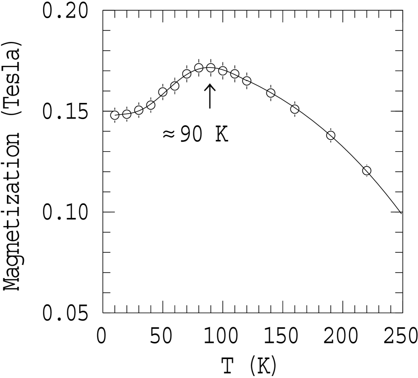
Figure 2: Measured magnetization as a function of temperature for a 5.3 mg/cm² gadolinium foil [12]. The line is drawn to guide the eye and the error bars represent the uncertainty in the absolute magnetization. The external polarizing field was 0.09 T. This magnetization curve is very similar to that of a single crystal magnetized along the $b$ axis [14]. The arrow indicates the approximate temperature at which many in-beam measurements are performed.

5 Unperturbed angular correlations

5.1 Formalism

The theoretical expression for the unperturbed angular correlation after Coulomb excitation can be written as (see Ref. [29, 30] and references therein)

$$W(\theta_{\gamma},\phi_{\gamma})=\sum_{k,q}\sqrt{(2k+1)}\langle\rho_{kq}(\theta,\phi)\rangle F_{k}Q_{k}D^{k*}_{q0}(\phi_{\gamma},\theta_{\gamma},0),$$ (4)

where $\langle\rho_{kq}(\theta,\phi)\rangle$ is the statistical tensor, which defines the spin alignment of the initial state, and which depends on the particle scattering angles $(\theta,\phi)$ and the geometry of the particle detector. $F_{k}$ represents the usual $F$-coefficients for the $\gamma$-ray transition, $Q_{k}$ is the attenuation factor for the finite size of the $\gamma$-ray detector, and $D^{k}_{q0}(\phi_{\gamma},\theta_{\gamma},0)$ is the rotation matrix, which depends on the $\gamma$-ray detection angles $(\theta_{\gamma},\phi_{\gamma})$. In the applications of interest $k=0,2,4$. The co-ordinate frame is right-handed with the beam along the positive $z$-axis as shown in Fig. 3. In the present work the $\gamma$-ray detectors are in the $xz$ plane, thus $\phi_{\gamma}=0$, and the rotation matrix is equivalent to an associated Legendre polynomial. The statistical tensors, and hence the unperturbed angular correlations, can be calculated accurately for the reaction geometry using the theory of Coulomb excitation.

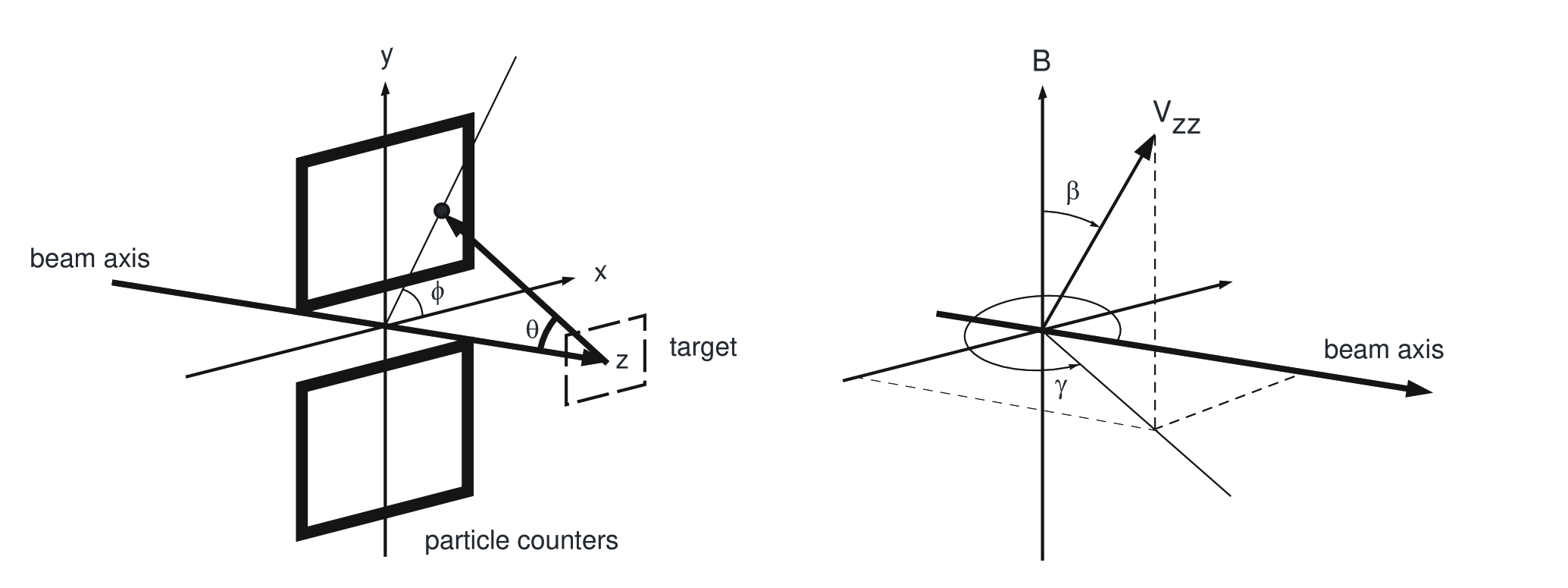
Figure 3: Left: Schematic of particle detector defining the co-ordinate frame. The beam is along the $z$-axis and the magnetic field direction is along the $y$-axis. The $\gamma$-ray detectors are in the $xz$-plane. Right: Definitions of the spherical polar angles $(\beta,\gamma)$ which specify the direction of the electric field gradient (EFG), $\bm{V}_{zz}$, with respect to the magnetic field direction and the beam axis. The EFG in the gadolinium target foils studied here is aligned predominantly along the beam axis, i.e. $\beta=90^{\circ}$, $\gamma=0^{\circ}$.

The Coulomb excitation calculations performed here are based on the de Boer-Winther code [31]. In this code the statistical tensors are evaluated in the particle-scattering plane. To calculate the angular correlations requires the tensors corresponding to scattering at angle $\phi$ as defined in Fig. 3. These are given by

$$\rho_{kq}(\theta,\phi) = \sum_{q^{\prime}}\rho_{kq^{\prime}}(\theta,0)D^{k}_{q^{\prime}q}(\phi,0,0)$$ (5)

$$= \rho_{kq}(\theta,0){\rm e}^{iq\phi},$$ (6)

where $\rho_{kq}(\theta,0)$ are from the de Boer-Winther calculation. Thus the required average statistical tensor at a given beam energy is given by

$$\langle\rho_{kq}\rangle=\frac{\int_{\theta}\int_{\phi}\rho_{kq}(\theta,0){\rm e}^{iq\phi}\frac{{\rm d}\sigma}{{\rm d}\Omega}{\rm d}\Omega}{\int_{\theta}\int_{\phi}\frac{{\rm d}\sigma}{{\rm d}\Omega}{\rm d}\Omega},$$ (7)

where the integrals are over the dimensions of the particle detector and $\frac{{\rm d}\sigma}{{\rm d}\Omega}$ is the cross section for Coulomb excitation corresponding to the scattering angle $\theta$. In the geometry used here (Fig. 3) there are two particle detectors placed symmetrically about the beam axis such that the numerical integration can be limited to the positive quadrant, $0^{\circ}\leq\phi\leq 90^{\circ}$. The factor ${\rm e}^{iq\phi}$ can then be replaced by $({\rm e}^{iq\phi}+{\rm e}^{-iq\phi}+{\rm e}^{iq(\phi+\pi)}+{\rm e}^{-iq(\phi+\pi)})/4$, which is $\cos q\phi$ if $q$ is even and is zero if $q$ is odd.

To obtain the statistical tensors of direct relevance to the present experiments, a further integration was performed to average over the energy loss of the beam in the target. A correction for feeding from higher states in the ground-state band was also made. Since the feeding path is only along the ground-state band, the statistical tensor of the fed state $i$ can be evaluated iteratively using

$$\rho^{\rm fed}_{kq}(i)=\frac{\rho_{kq}(i)P^{\rm direct}(i)+U_{k}(i+1\rightarrow i)\rho^{\rm fed}_{kq}(i+1)P^{\rm total}(i+1)}{P^{\rm direct}(i)+P^{\rm total}(i+1)},$$ (8)

where $\rho_{kq}(i)$ is the unfed statistical tensor for the state and $P^{\rm direct}(i)$ is the direct population of the state by Coulomb excitation. $P^{\rm total}(i+1)$ is the total population of the ground-band level above level $i$, including direct excitation and feeding contributions, if any. $U_{k}(i+1\rightarrow i)$ is the $U$-coefficient for the $i+1\rightarrow i$ transition [32]. These feeding corrections are small in the present work. In all cases feeding from states with $I>2$ in the ground-state band contributes less than 7% of the total intensity in the $2^{+}_{1}\rightarrow 0^{+}_{1}$ transition.

The resultant nonzero statistical tensors for the 2${}^{+}_{1}$ state of ¹⁵⁶Gd are shown in Table 6. For an annular counter only the $q=0$ tensors are non zero. The broken azimuthal symmetry gives rise to the finite $\rho_{kq}$ values for $q\neq 0$, however these terms are small in the present case because the scattering angle remains near 180^∘ and the spin of the excited state is aligned predominantly in the plane perpendicular to the beam.

Table 6: Statistical tensors for the 2${}^{+}_{1}$ state of ¹⁵⁶Gd.

$k$	$q$	$\rho_{k,q}$
0	0	1.0000
2	2	0.0061
2	0	-0.5033
4	4	0.0002
4	2	-0.0304
4	0	0.4404

5.2 Angular correlation results and discussion

Figures 4 and 5 show examples of comparisons between the calculated unperturbed angular correlations and the data. The angular correlations for the $2^{+}_{1}\rightarrow 0^{+}_{1}$ transitions shown in Fig. 4 were obtained at room temperature (run I), above the Curie temperature. Thus there is no magnetic-dipole perturbation, but there is expected to be an electric field gradient (EFG). In Fig. 4 the dotted lines indicate the angular correlation anticipated for a target with the expected electric field gradient of $V_{zz}=3.44\times 10^{17}$ V/cm² distributed isotropically. There is no evidence for any attenuation of the anisotropy due to electric field gradients. This observation again confirms that these rolled and annealed foils have a texture such that the basal planes are perpendicular to the beam, in the plane of the foil. There is no perturbation because the $c$ axis, and hence the EFG, is along the beam direction, perpendicular to the plane of spin alignment.

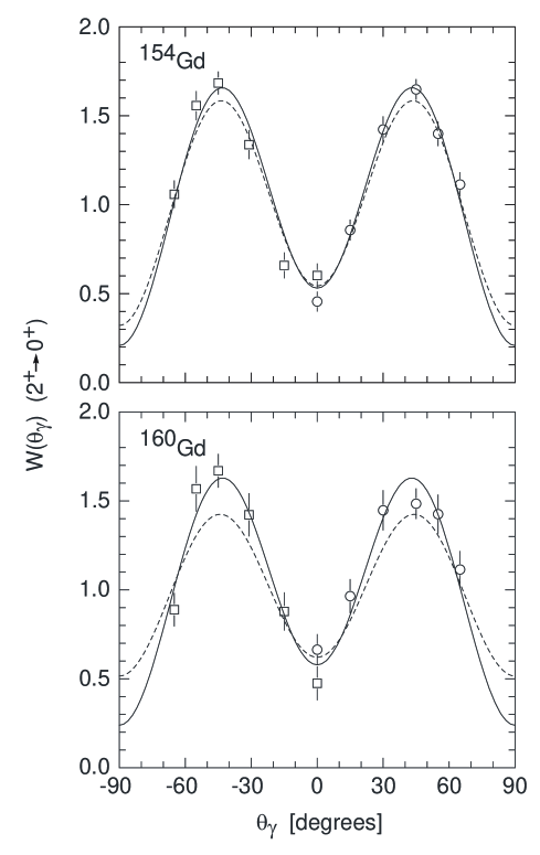
Figure 4: Unperturbed angular correlations for the $2^{+}_{1}\rightarrow 0^{+}_{1}$ transitions in ¹⁵⁴Gd and ¹⁵⁶Gd. Circles (squares) represent data taken with the detector in the positive (negative) quadrant. The solid line is the theoretical angular correlation given by Eq. (4). The dotted line shows the effect of an isotropic electric-field gradient ($V_{zz}=3.44\times 10^{17}$ V/cm²). The good agreement between the data and the solid lines implies that the electric-field gradient is predominantly directed along the beam direction, and hence that the gadolinium foil is a quasi single crystal with the $c$ axis perpendicular to the plane of the foil.

Figure 5: Unperturbed angular correlations for the $4^{+}_{1}\rightarrow 2^{+}_{1}$ transitions in ^156,158,160Gd. Circles and squares represent data taken at room temperature in run II. The triangles represent data taken at a nominal target temperature of 90 K in run III. As in Fig. 4 different symbols are used to designate data taken with the detectors in the positive and negative quadrants.

The data shown for the $4^{+}_{1}\rightarrow 2^{+}_{1}$ transitions in Fig. 5 include data obtained at both room temperature and at 90 K (runs I and II), where magnetic perturbations are present. The calculated and measured angular correlations are in agreement. There is no observable difference between the measurements at 90 K and 300 K because the unperturbed angular correlations can be recovered by adding together the data for both directions of the external field. This procedure cancels out the relatively small rotation of the radiation pattern which changes direction when the external field direction is reversed. (The same procedure cannot be applied for the 2${}^{+}_{1}$ states because the perturbations are much too large.)

6 Perturbed angular correlations

6.1 Formalism

Since the perturbation of the angular correlation stems from changes in the distribution of the nuclear spins as specified by changes in the statistical tensors, the expression for the perturbed angular correlation has the same form as Eq. (4), with the statistical tensors $\langle\rho_{kq}\rangle$ replaced by values that correspond to the perturbed spin distribution. The effect of the transient-field precession, which acts as a pure rotation around the direction of the magnetic field, is applied first. As shown in Fig. 3, the magnetic field is directed along the $y$-axis. The statistical tensor therefore becomes

$$\rho_{kq}=\sum_{Q}\langle\rho_{kQ}\rangle D^{k}_{qQ}(0,\Delta\theta_{\rm tf},0),$$ (9)

where $\langle\rho_{kQ}\rangle$ are the unperturbed tensors. The sign of $\Delta\theta_{\rm tf}$ is reversed when the direction of the polarizing field is reversed.

After the transient-field precession has been applied, a combined electric-quadrupole and magnetic-dipole interaction, due to the static fields in the gadolinium host matrix, is allowed to perturb the statistical tensor. The perturbed tensors, $\rho_{k^{\prime}q^{\prime}}$, are derived from the tensors, $\rho_{kq}$, using

$$\rho_{k^{\prime}q^{\prime}}=\sum_{k,q}\rho_{k,q}[G^{qq^{\prime}}_{kk^{\prime}}]^{*}\sqrt{\frac{(2k+1)}{(2k^{\prime}+1)}},$$ (10)

where $[G^{qq^{\prime}}_{kk^{\prime}}]^{*}$ is the perturbation factor for the combined magnetic and electric hyperfine interactions. $[G^{qq^{\prime}}_{kk^{\prime}}]^{*}$ can be related to the perturbation factors denoted ${\rm III}^{qq^{\prime}}_{kk^{\prime}}(\beta,\gamma)$, given by Alder et al. [33, 34] for combined electric and magnetic interactions:

$$[G^{qq^{\prime}}_{kk^{\prime}}(t)]^{*}=\frac{\sqrt{(2k+1)(2k^{\prime}+1)}}{(2I+1)}\sum_{Q,Q^{\prime}}D^{k*}_{qQ}(\frac{\pi}{2},\frac{\pi}{2},\pi){\rm III}^{QQ^{\prime}}_{kk^{\prime}}(\beta,\gamma)D^{k^{\prime}}_{q^{\prime}Q^{\prime}}(\frac{\pi}{2},\frac{\pi}{2},\pi).$$ (11)

The Euler (or spherical polar) angles $(\beta,\gamma)$ specify the orientation of the electric field gradient with respect to the magnetic field direction, which is along the $y$ axis in Fig. 3. $\beta$ is the polar angle between the directions of the magnetic field and the electric-field gradient. The azimuthal angle $\gamma$ is measured from the beam axis in the horizontal plane, i.e. the $xz$-plane in Fig. 3. Although it is not usually written explicitly, ${\rm III}^{QQ^{\prime}}_{kk^{\prime}}(\beta,\gamma)$ is a function of $\omega\tau$ and $\omega_{Q}\tau$, where $\omega\tau$ is the magnetic dipole precession angle as defined above and $\omega_{Q}\tau$ is the electric quadrupole precession, where $\omega_{Q}$ is

$$\omega_{Q}=\frac{eQV_{zz}}{4I(2I-1)\hbar}.$$ (12)

6.2 Data analysis procedures

As a first approximation, the experimental total precession angles for the 4${}^{+}_{1}$ states, $\Delta\Theta$, can be extracted from the field-up/field-down data by conventional procedures [5, 13] in which the experimental precession angle is related to the field up/down counting asymmetry $\epsilon$ by the expression

$$\Delta\Theta={\epsilon}/{S},$$ (13)

where $S=(1/W)(dW/d\theta)$ is the logarithmic derivative of the angular correlation at the detection angle $+\theta_{\gamma}$ and

$$\epsilon=(1-\rho)/(1+\rho).$$ (14)

The ‘double ratio’ $\rho$ is derived from the counting rates in the detectors at $\pm\theta_{\gamma}$, $N(\pm\theta_{\gamma})$, for field up ($\uparrow$) and down ($\downarrow$) by

$$\rho=\sqrt{\frac{N(+\theta_{\gamma},\uparrow)}{N(+\theta_{\gamma},\downarrow)}\frac{N(-\theta_{\gamma},\downarrow)}{N(-\theta_{\gamma},\uparrow)}}.$$ (15)

Note that the factors due to integrated beam current, cross sections and detector efficiencies cancel out so that

$$\rho=W(+\theta_{\gamma},\uparrow)/W(+\theta_{\gamma},\downarrow)$$ (16)

and hence $\epsilon$ is formally equivalent to

$$\epsilon(\theta_{\gamma})=\frac{W(+\theta_{\gamma},\downarrow)-W(+\theta_{\gamma},\uparrow)}{W(+\theta_{\gamma},\downarrow)+W(+\theta_{\gamma},\uparrow)}.$$ (17)

For the longer-lived 2${}^{+}_{1}$ states, where the perturbations are much larger, this procedure does not apply. Indeed, it also underestimates the precessions of the 4${}^{+}_{1}$ states by up to $\sim 10\%$. The procedure used here to analyze both the 2${}^{+}_{1}$ and 4${}^{+}_{1}$ data is to begin by forming the experimental double ratio, $\rho$, and asymmetry parameter $\epsilon$ as usual, so that the beam current, cross section and efficiency factors cancel. The experimental value of $\omega\tau$ is then extracted by fitting the experimental values of $\epsilon$ (Eq. (14) and Eq. (15)) to theoretical values of $\epsilon$ evaluated using Eq. (17).

6.3 Electric quadrupole and magnetic dipole perturbations

The combined effect of electric quadrupole and magnetic dipole interactions on the angular correlation and the asymmetry $\epsilon$ is explored in Figs. 6-8.

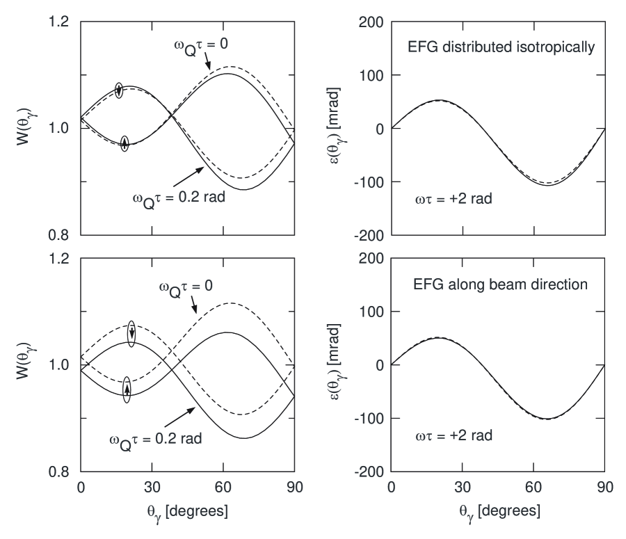
Figure 6: Perturbed angular correlations for a hypothetical $2^{+}_{1}\rightarrow 0^{+}_{1}$ transition which experiences a combined magnetic-dipole and electric-quadrupole interaction. The left-hand panels show the angular correlation, $W(\theta_{\gamma})$, while the right-hand panels show the asymmetry, $\epsilon(\theta_{\gamma})$, derived from double ratios as described in the text concerning Eq.(14) and Eq.(15). In all panels the magnetic precession is $\omega\tau=+2$ rad for ‘field up’. The field directions are indicated by the arrows. Solid lines show the case where an electric-field gradient, which causes a quadrupole precession of $\omega_{Q}\tau=0.2$ rad, is also present. For reference the dotted lines show the $\omega_{Q}\tau=0$ case. In the upper two panels the electric-field gradient is distributed isotropically, while in the lower panels it is directed along the beam axis, as is the case in the present measurements.

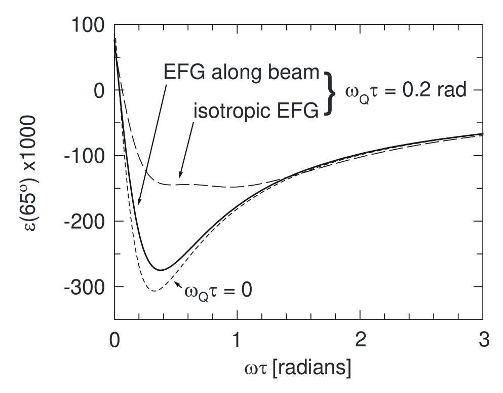
Figure 7: Asymmetry, $\epsilon(65^{\circ})$, for a typical $2^{+}\rightarrow 0^{+}$ transition, as a function of the magnetic precession angle $\omega\tau$ when an electric-quadrupole precession of $\omega_{Q}\tau=0.2$ rad is present, either distributed isotropically or directed along the beam direction (as is the case in the present work). The case of $\omega_{Q}\tau=0$ is shown for reference. In the present work the $\omega\tau$ values lie between $\sim 0.8$ and $\sim 2.2$ rad, with $\omega_{Q}\tau=0.2$ being applicable when $\omega\tau\sim 2.5$ rad. See also Fig. 8.

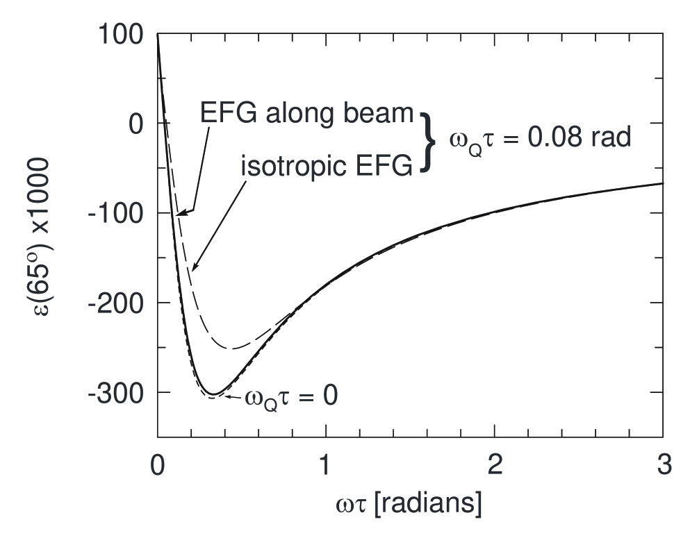
Figure 8: As for Fig. 7, but for $\omega_{Q}\tau=0.08$ rad. In the present work $\omega_{Q}\tau=0.08$ rad is associated with $\omega\tau\sim 0.8$ rad.

In Fig. 6, the transient-field precession, which is relatively small, was set to zero, the magnetic dipole precession angle was $\omega\tau=2$ rad, and the electric quadrupole precession was $\omega_{Q}\tau=0.2$ rad. These values are near those for ¹⁶⁰Gd in the data presented below. Two extreme cases are shown. In the upper panels of Fig. 6 the EFG is assumed to be distributed isotropically, while in the lower panels it is directed along the beam axis. As discussed above, the latter case is very close to the real situation. Although the electric field gradient is directed along the beam axis, perpendicular to the initial spin orientation, such that it cannot perturb the angular correlation on its own, it can have an observable effect on the perturbed angular correlation when the magnetic dipole interaction is also present, because the magnetic interaction moves the nuclear spin out of the plane perpendicular to the beam. Thus the perturbed angular correlations shown in the left panels of Fig. 6 differ, depending on the direction and magnitude of the electric field gradient.

Figures 7 and 8 show the dependence of the asymmetry $\epsilon(65^{\circ})$ on the magnitude of the magnetic perturbation $\omega\tau$ for a given strength of the quadrupole interaction. In these figures a realistic value of the transient-field precession was included, $\Delta\theta=-40$ mrad, where the negative sign applies for ‘field up’. The value $\omega_{Q}\tau=0.2$ rad was chosen because it is slightly larger than the value applicable for ¹⁶⁰Gd, the largest considered here; $\omega_{Q}\tau=0.08$ rad is slightly larger than the value for ¹⁵⁴Gd. The effect of the electric-field gradient is apparent in the region up to $\omega\tau\approx 1$ rad when the EFG is isotropically distributed. However when $\omega\tau>>\omega_{Q}\tau$, the asymmetries, $\epsilon(65^{\circ})$, are hardly affected, especially when the EFG is directed along the beam direction.

In the following analysis $\omega\tau$ values are extracted assuming the EFG is directed along the beam direction, as was shown to apply for our foils in Sections 4 and 5. $\omega_{Q}$ was evaluated assuming the electric-field gradient from Ref. [2] and the experimental quadrupole moments in Table 4. The parameters of the EFG are not critical, however. In all cases considered here essentially the same $\omega\tau$ values would be extracted if EFG effects were assumed isotropic or even ignored altogether.

6.4 Nuclei on damaged sites

The analysis procedures described above implicitly assume that all of the implanted nuclei experience the same hyperfine magnetic field and the same electric-field gradient. It is well known, however, that after implantation into metals typically 5 - 10% of the implanted nuclei reside on damaged sites and therefore do not experience the same hyperfine fields as those on substitutional sites.

It will become apparent in the following that an analysis of the present data assuming a unique implantation site leads to a contradiction between the effective fields experienced by the 4⁺ and 2⁺ states. A two-site analysis is necessary to resolve this contradiction.

For the analysis of integral perturbed angular correlations it is usually sufficient to assume a two-site model in which the damaged sites have no static hyperfine magnetic field. This assumption will be adopted here with the additional assumption that there is also no net electric field gradient on the damaged sites. It will become apparent in the following discussion that these assumptions are not critical because the number of damaged sites is small.

In a two-site model with a fraction of nuclei $f$ on field-free sites after implantation, the perturbed angular correlation, $W(\Delta\theta_{\rm tf},\omega\tau,\omega_{Q}\tau)$ is replaced by

$$(1-f)W(\Delta\theta_{\rm tf},\omega\tau,\omega_{Q}\tau)+fW(\Delta\theta_{\rm tf},0,0).$$ (18)

Note that the nuclei that end up on field-free sites still experience the transient field as they slow in the ferromagnetic medium, but they do not experience any hyperfine interactions after they come to rest.

The effect of a fraction of damaged sites on the observed asymmetry $\epsilon(65^{\circ})$ is demonstrated in Fig. 9. In the present case a fraction of nuclei on field-free sites, which is not taken into account, gives an apparently enhanced $B_{\rm st}$ for the 2⁺ states and an apparently reduced $B_{\rm st}$ for the 4⁺ states. The difference comes about because the longer-lived 2⁺ states are in the region where an increase in $\omega\tau$ results in a decrease in the magnitude of $\epsilon$ whereas for the 4⁺ states an increase in $\omega\tau$ results in an increase in the magnitude of $\epsilon$.

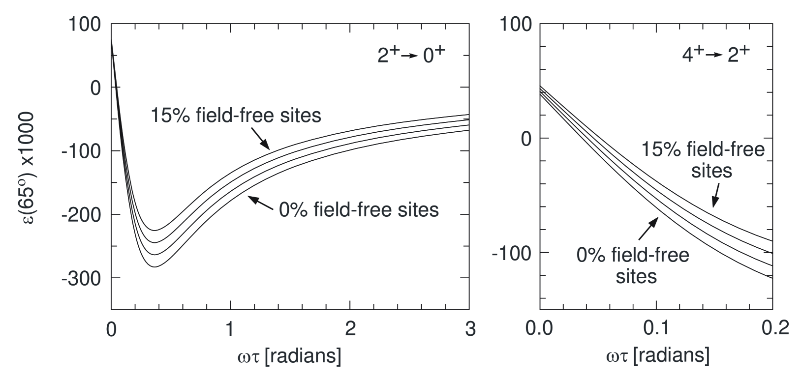
Figure 9: Asymmetry, $\epsilon(65^{\circ})$, for typical $2^{+}\rightarrow 0^{+}$ and $4^{+}\rightarrow 2^{+}$ transitions, as a function of the magnetic precession angle $\omega\tau$ when a fraction of the implanted nuclei reside on field-free sites. Calculations are shown for field-free fractions from 0% to 15% in 5% steps.

Table 7: Summary of 2⁺ precessions.

Run	$\Delta\theta_{\rm tf}$	$\omega_{Q}\tau$	$\epsilon(65^{\circ})\times 10^{3}$	$\omega\tau(65^{\circ})$		$\epsilon(120^{\circ})\times 10^{3}$	$\omega\tau(120^{\circ})$		$\langle\omega\tau\rangle$
	(mrad)	(mrad)		(mrad)			(mrad)		(mrad)
				1-site	2-site		1-site	2-site	1-site	2-site
154Gd
II	$-35$	67	$-204(14)$	904${}^{+88}_{-78}$	698${}^{+75}_{-69}$	221(16)	784${}^{+94}_{-86}$	537${}^{+90}_{-103}$	849${}^{+64}_{-58}$	640${}^{+58}_{-57}$
III	$-43$	67	$-193(10)$	956${}^{+68}_{-62}$	828${}^{+61}_{-57}$	180(16)	1030${}^{+133}_{-115}$	865${}^{+117}_{-103}$	972${}^{+61}_{-55}$	836${}^{+54}_{-50}$
IV	$-43$	67	$-187(11)$	995${}^{+80}_{-72}$	863${}^{+71}_{-65}$	153(13)	1242${}^{+144}_{-123}$	1073${}^{+123}_{-107}$	1062${}^{+70}_{-62}$	918${}^{+61}_{-56}$
156Gd
II	$-31$	139	$-148(8)$	1299${}^{+87}_{-79}$	1039${}^{+71}_{-64}$	130(7)	1529${}^{+101}_{-91}$	1168${}^{+78}_{-70}$	1397${}^{+66}_{-60}$	1098${}^{+53}_{-47}$
III	$-39$	139	$-120(5)$	1635${}^{+80}_{-74}$	1435${}^{+69}_{-64}$	117(7)	1706${}^{+125}_{-111}$	1456${}^{+105}_{-94}$	1657${}^{+67}_{-62}$	1441${}^{+58}_{-53}$
IV	$-39$	139	$-107(5)$	1858${}^{+100}_{-92}$	1626${}^{+86}_{-79}$	113(7)	1775${}^{+133}_{-118}$	1514${}^{+112}_{-100}$	1827${}^{+80}_{-73}$	1584${}^{+68}_{-62}$
158Gd
II	$-31$	165	$-123(11)$	1588${}^{+176}_{-148}$	1274${}^{+140}_{-119}$	107(8)	1893${}^{+172}_{-148}$	1447${}^{+129}_{-112}$	1742${}^{+123}_{-105}$	1367${}^{+95}_{-82}$
III	$-38$	165	$-100(6)$	1984${}^{+139}_{-123}$	1740${}^{+119}_{-106}$	94(9)	2168${}^{+254}_{-210}$	1848${}^{+210}_{-176}$	2029${}^{+122}_{-106}$	1767${}^{+104}_{-91}$
IV	$-38$	165	$-91(8)$	2198${}^{+229}_{-193}$	1922${}^{+193}_{-164}$	101(8)	2001${}^{+193}_{-165}$	1709${}^{+161}_{-139}$	2084${}^{+148}_{-125}$	1797${}^{+124}_{-106}$
160Gd
II	$-30$	177	$-111(12)$	1770${}^{+238}_{-193}$	1424${}^{+188}_{-154}$	101(10)	2010${}^{+246}_{-202}$	1541${}^{+184}_{-153}$	1885${}^{+171}_{-140}$	1483${}^{+131}_{-109}$
III	$-36$	177	$-87(7)$	2298${}^{+216}_{-185}$	2016${}^{+184}_{-158}$	112(11)	1774${}^{+220}_{-182}$	1524${}^{+186}_{-154}$	2036${}^{+154}_{-130}$	1768${}^{+131}_{-110}$
IV	$-36$	177	$-73(8)$	2770${}^{+360}_{-290}$	2415${}^{+299}_{-244}$	104(10)	1929${}^{+231}_{-191}$	1656${}^{+195}_{-162}$	2179${}^{+194}_{-160}$	1885${}^{+163}_{-135}$

6.5 Results: 2${}^{+}_{1}$ states

Table LABEL:tab:2+results summarizes the results of the present measurements of the static-field precessions for the 2${}^{+}_{1}$ states in ^{154,156,158,160}Gd. The data were analyzed adopting both a single-site model (i.e. $f=0$ in Eq. (18)) and a two site model ($f\neq 0$). The procedure by which the field-free fraction was determined for the two site-model analysis is described in section 6.7.

While the $\omega\tau$ values Table LABEL:tab:2+results were extracted exclusively from the asymmetries, $\epsilon(65^{\circ})$ and $\epsilon(120^{\circ})$, these values are consistent with the full perturbed angular correlations, where measured. For example, the perturbed angular correlation data for ¹⁵⁴Gd and ¹⁵⁶Gd measured in run II are shown in Fig. 10, and compared with the perturbed angular correlations corresponding to the $\omega\tau$ values for the single-site model (see Table LABEL:tab:2+results).

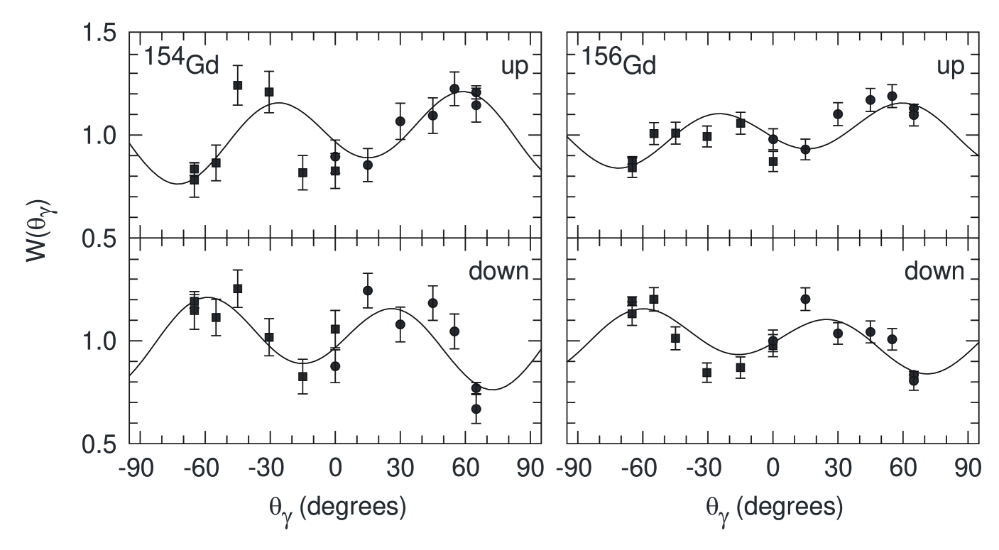
Figure 10: Perturbed angular correlations for the $2^{+}_{1}\rightarrow 0^{+}_{1}$ transitions in ¹⁵⁴Gd and ¹⁵⁶Gd measured in run II. The solid curves are calculated for the average single-site $\omega\tau$ values in Table LABEL:tab:2+results. These data make it clear that the $\omega\tau$ values for the 2${}^{+}_{1}$ states are much larger than 0.5 rad.

To some extent the extracted magnetic-dipole precession angles, $\omega\tau$, depend on the assumed transient-field precession angle, $\Delta\theta_{\rm tf}$, and the quadrupole precession, $\omega_{Q}\tau$. Figures 6 and 8 discussed in the previous subsection show that $\omega\tau$ is very insensitive to reasonable assumed values of $\omega_{Q}\tau$. The effect of the transient-field contribution is somewhat counter intuitive at first sight: $\omega\tau$ decreases by $\sim 20$ mrad when the magnitude of $\Delta\theta_{\rm tf}$ (which is negative) increases by 10 mrad. (See Fig. 4 in Ref. [35] for a plot of $\epsilon$ versus $\omega\tau$ showing the effect of the transient-field contribution.) Because the $\omega\tau$ values are so large, however, an increase in $\Delta\theta_{\rm tf}$ by $\sim 50$% would lead to a change in $\omega\tau$ for ¹⁵⁴Gd (¹⁶⁰Gd) by only $\sim 4$% ($\sim 2$%).

A fixed value of $\Delta\theta_{\rm tf}/g=-100$ mrad was adopted for run IV, and scaled according to the foil magnetization for runs II and III as obtained in a preliminary fit to the data. This value was chosen because it is consistent with the previous data [1] once a correction is made for the difference in Gd recoil velocities due to the difference in the beam energies. In principle, $\Delta\theta_{\rm tf}$ could be obtained from the data for the 4⁺ states. Unfortunately, however, the present data for the 4⁺ states are not sufficiently precise to fit both the static- and transient-field precessions as free parameters (see below).

Results presented for the two-site model assume a field-free fraction of 11.6% in run II and 6.4% in runs III and IV. These values were determined by requiring consistency between the extracted static-field strengths for the 2${}^{+}_{1}$ and 4${}^{+}_{1}$ states, as described in section 6.7.

The effective static-field strengths derived from the average precession angles given in Table LABEL:tab:2+results are summarized in Table 8. As will be discussed below, the differences in these effective static-field strengths from run to run are attributed to changes in the magnetization of the gadolinium foil target associated with different foil textures and different beam heating effects.

Table 8: Effective static-field strengths derived from 2⁺-state precessions.

Nucleus	$B_{\rm st}$ (Tesla) Single-site analysis				$B_{\rm st}$ (Tesla) Two-site analysis
	Run II (A)	Run III (A)	Run IV (B)		Run II (A)	Run III (A)	Run IV (B)
154Gd	$-24.1$(2.4)	$-27.6$(2.5)	$-30.2$(2.8)		$-18.2(2.1)$	$-23.8(2.2)$	$-26.1(2.5)$
156Gd	$-23.1$(1.1)	$-27.4$(1.2)	$-30.2$(1.4)		$-18.1(0.9)$	$-23.8(1.0)$	$-26.2(1.2)$
158Gd	$-25.6$(1.8)	$-29.8$(1.8)	$-30.6$(2.1)		$-20.1(1.4)$	$-26.0(1.5)$	$-26.4(1.8)$
160Gd	$-27.7$(2.7)	$-29.9$(2.6)	$-32.0$(3.1)		$-21.8(2.1)$	$-26.0(2.2)$	$-27.7(2.6)$
average	$-24.3$(0.8)	$-28.3$(0.9)	$-30.5$(1.0)		$-19.0$(0.7)	$-24.6$(0.8)	$-26.4$(0.9)

6.6 Results: 4${}^{+}_{1}$ states

Table 9 summarizes the results of the present measurements on the 4${}^{+}_{1}$ states in ^156,158,160Gd. The 4⁺ state in ¹⁵⁴Gd was populated too weakly in the present work to be analyzed. The precession angles $\omega\tau$ were obtained by the rigorous procedure described in section 6.2 assuming the same $\Delta\theta_{\rm tf}$ values as adopted for the analysis of the 2${}^{+}_{1}$ states (Table LABEL:tab:2+results).

Table 9: Summary of 4${}^{+}_{1}$ state precessions.

Run	Target	$\Delta\theta_{\rm tf}$	$\epsilon(65^{\circ})$	$\epsilon(120^{\circ})$	$\langle\omega\tau\rangle$		$\langle\Delta\Theta\rangle/g$
			$(\times 10^{3}$)	$(\times 10^{3}$)	(mrad)		(mrad)
					1-site	2-site	1-site
156Gd
II	A	$-31$	$-$40(12)	1(12)	50(9)	56(10)	52(25)
III	A	$-39$	$-$21(10)	24(14)	61(8)	65(9)	58(21)
IV	B	$-39$	$-$26(10)	5(12)	56(8)	60(8)	44(21)
158Gd
II	A	$-31$	$-$38(10)	35(10)	68(7)	77(9)	102(20)
III	A	$-38$	$-$55(8)	59(12)	97(8)	105(9)	155(21)
IV	B	$-38$	$-$65(8)	65(10)	108(8)	117(9)	181(21)
160Gda
II	A	$-30$	$-$36(10)	49(11)	72(8)	82(9)	115(23)
III	A	$-36$	$-$64(9)	48(13)	96(9)	104(10)	157(24)
IV	B	$-36$	$-$84(9)	64(10)	117(9)	126(10)	209(23)
a A correction has been applied to account for a $\sim 8$% contribution to the intensity of the $4^{+}\rightarrow 2^{+}$ transition in 160Gd due to the $9/2^{-}\rightarrow 7/2^{-}$ transition in 157Gd.

Figure 11: Left: Previous precession results, $\Delta\Theta/g$, for the 4${}^{+}_{1}$ and 6${}^{+}_{1}$ states in the even Gd isotopes [1] plotted as a function of the mean level lifetime $\tau$. These data were obtained following Coulomb excitation with 56 MeV ¹⁶O beams. Right: Present data for 4${}^{+}_{1}$ states in ^156,158,160Gd from run IV, obtained with 40 MeV ¹⁶O beams. In both panels, the solid line, for $B_{\rm st}=-25$ T, is the best fit to the data. The dotted line forces the static field strength to be $-30$ T as implied by the single-site analysis of the data for the 2${}^{+}_{1}$ states.

If both sides of Eq. (1) are divided by $g$ it becomes

$$\Delta\Theta/g=(\omega/g)\tau+\Delta\theta_{\rm tf}/g.$$ (19)

From this equation it can be seen that a plot of $\Delta\Theta/g$ values versus $\tau$ should lie on a straight line with a slope $\omega/g$, which is proportional to $B_{\rm st}$, and with an intercept $\Delta\theta_{\rm tf}/g$ at $\tau=0$. To aid comparison with previous work, the final column of Table 9 shows the total precessions, $\Delta\Theta$, according to the single-site model. The left panel of Fig. 11 shows the previous data, from [1], for the 4${}^{+}_{1}$ and 6${}^{+}_{1}$ states in the even Gd isotopes so plotted. For comparison the right panel shows the present data for the 4${}^{+}_{1}$ states from run IV (single-site analysis). The results of the previous work [1] have been reanalyzed using the present adopted $g$ factor and lifetime values (Tables 3 and 4). These previous data were fitted treating both $\omega/g$ and $\Delta\theta_{\rm tf}/g$ as free parameters. The result, shown as the solid line in the left panel of Fig. 11, corresponds to $B_{\rm st}=-25(3)$ T, in agreement with the value of $-25$ T obtained in run IV (single-site analysis).

Unfortunately the present data for the 4${}^{+}_{1}$ states are not sufficiently precise to fit both the slope and the intercept as free parameters. The transient-field precession was therefore set to the values adopted in the analysis of the 2⁺ states (see Table LABEL:tab:2+results). These values and the extracted static-field strengths for the one- and two-site models are presented in Table 10.

Table 10: Hyperfine fields extracted from 4${}^{+}_{1}$ state precessions.

Run	Target	$\Delta\theta_{\rm tf}/g$	$B_{\rm st}$
		(mrad)	(Tesla)
			1-site	2-site
Ref. [1]		$-136(26)$	$-25(3)$
II	A	$-80$	$-16.7(1.3)^{a}$	$-19.0(1.4)^{a}$
III	A	$-93$	$-22.7(1.4)^{a}$	$-24.4(1.5)^{a}$
IV	B	$-100$	$-24.7(1.4)^{a}$	$-26.7(1.5)^{a}$
a The uncertainty in the transient-field contribution is not included in the quoted error.

Since the previous measurements [1] were made with 56 MeV ¹⁶O beams, somewhat higher than the 40 MeV beams used here, the transient-field contribution must be larger in the previous work. According to the Rutgers [36] and Chalk River [6] parametrizations, the expected difference in $\Delta\theta_{\rm tf}/g$ is about 30 mrad. As shown in Table 10, the present data for target B in run IV (single-site analysis) are consistent both with the expected difference in transient-field precession and with the same static field strength as observed in Ref. [1]. The present measurements from run IV are also in agreement with the static-field strengths obtained by Häusser et al. [6].

All of the previous work has assumed a single-site for the implanted nuclei. However a comparison of the results in Tables 8 and 10 shows that the assumption of a single implantation site implies that the effective static-field strengths for the 4${}^{+}_{1}$ states are significantly smaller than those experienced by the 2${}^{+}_{1}$ states.

6.7 The field-free fraction

Figure 12 illustrates the procedure used to determine the field-free fraction $f$, according to the two-site model described in section 6.4. In order to achieve consistent $B_{\rm st}$ values for the 2⁺ and 4⁺ states requires that in run II, 11.6${}^{+2.7}_{-2.3}$% of the implanted nuclei reside on field-free sites. In runs III and IV, the field-free fractions are 6.7${}^{+1.9}_{-1.8}$% and 6.1${}^{+1.8}_{-1.7}$%, respectively, giving an average of $6.4\pm 1.3$%. Thus the two-site analysis adopted $f=0.116$ for run III and $f=0.064$ for runs III and IV. The initial expectation would be that $f$ should be the same for all three runs. It is not clear why a higher percentage of ions apparently reside on damaged sites in run II. Since the hyperfine fields experienced by the implanted nuclei in run II are very different from those in runs III and IV, this difference might indicate that there is another effect associated with the perturbed angular correlations that has not been taken into account. The apparently different value of $f$ was retained for the two-site analysis of run II, subject to the caveat that it might not represent the true field-free fraction.

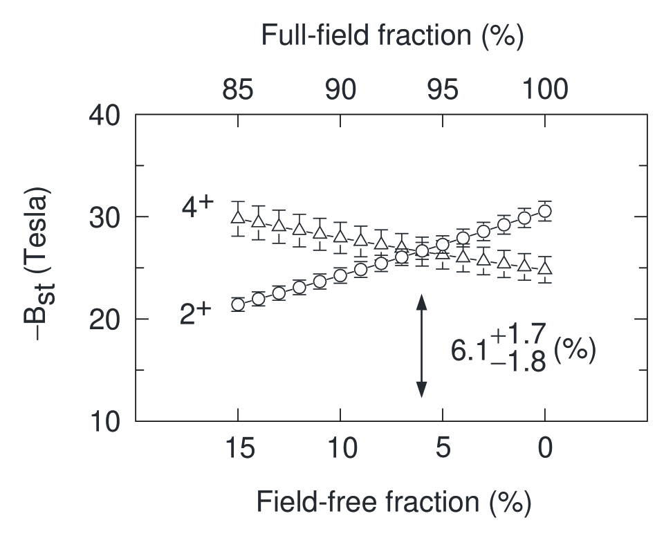
Figure 12: Determination of the field-free fraction for run IV.

7 Discussion

7.1 Synopsis

The primary motivation for the present measurements was to obtain an in-beam measure of the local magnetization of the gadolinium target foils, which can vary from foil to foil and for different beam-heating conditions. Clearly, the effective hyperfine field strength varies with the magnetization. The following discussion explores the extent to which ratios of effective fields can be interpreted as ratios of the host magnetizations.

Along with the presentation of the experimental data, the previous sections have established that the gadolinium foils used in the present experiments are quasi single crystals in which the electric-field gradient is directed along the beam direction (sections 4 and 5.2). It has been noted that the effect of the electric-field gradient is negligible for 4${}^{+}_{1}$ states. It has also been shown that, for the analysis procedures adopted here, the effect of the electric-field gradient along the beam direction is essentially negligible for the longer-lived 2 ${}^{+}_{1}$ states as well. It follows that the presence of the electric-field gradient does not impede the use of the effective static-field strength as a measure of the local magnetization.

Before coming to a discussion of the results in terms of the local magnetization and beam heating effects (section 7.3), it is necessary first to discuss the effect of the hyperfine field being misaligned with respect to the external field due to domain misalignment below the saturation magnetization (section 7.2).

7.2 Domain rotation below the saturation magnetization

It has been demonstrated for several impurities implanted into iron that internal hyperfine magnetic fields may be misaligned with respect to the direction of the external polarizing field, and that this effect is associated with domain rotation in an incompletely saturated sample [37]. At some level the effect is expected for all impurity-host combinations.

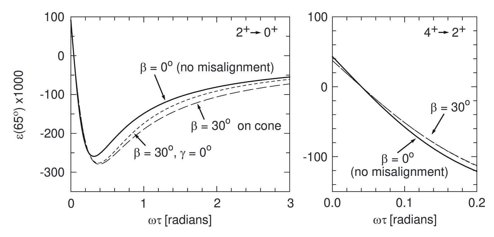
Figure 13: Asymmetry, $\epsilon(65^{\circ})$, as a function of $\omega\tau$ showing the effect of misalignment between the external field direction and the internal hyperfine field direction. The angles $\beta$ and $\gamma$, which specify the direction of the internal field, are defined as in Fig. 3. For the $4^{+}\rightarrow 2^{+}$ case the curves for $\beta=30^{\circ}$ on the cone and $\gamma=0^{\circ}$ are almost indistinguishable.

Figure 13 shows the effect of misaligned hyperfine fields on the analysis of the perturbed angular correlations. Two limiting cases of misaligned fields are assumed. In the first case the internal fields are assumed to lie on a cone of half angle $\beta=30^{\circ}$, whose axis is the external field direction. In the second case the internal field is assumed to lie in the plane defined by the beam axis and the external field direction, i.e. at angles $\beta=30^{\circ}$, $\gamma=0^{\circ}$ in terms of the co-ordinate frame in Fig. 3. Given that the gadolinium target has a texture such that it resembles a quasi single crystal with the $c$ axis along the beam, the latter case is likely to be more realistic in the present work. The formulae for evaluating these perturbed angular correlations are given in the Appendix.

It can be seen from Fig. 13 that if the internal field is misaligned with respect to the external field, then the true precession angle around the internal-field direction is always larger than that derived when no misalignment is assumed.

At least part of the difference between the effective static fields observed here and the Mössbauer result at 4 K ($B_{\rm st}=37.3(5)$ T [2]) is likely to be associated with misalignment between the internal and external fields. Indeed the subtle overall tendency for the effective static fields in Table 8 to increase slightly from ¹⁵⁴Gd to ¹⁶⁰Gd, as the 2${}^{+}_{1}$ state lifetimes and hence the $\omega\tau$ values increase, might be associated with misalignment between the internal and external fields, which has not been included in the analysis. (Note that the difference between the different curves in Fig. 13 decreases as $\omega\tau$ increases.) However the trend is below the statistical precision of the data.

It can be concluded that although the perturbed angular correlations may show some sensitivity to the direction of the internal field, the ratios of $\omega\tau$ values derived assuming that the internal and external fields are parallel can still be interpreted as magnetization ratios, to a very good approximation.

7.3 Beam heating and relative magnetizations of foils

There is no significant difference between the ratios of effective fields determined from the one-site or two-site analysis of the data. The following discussion will therefore use the ratios of the observed precession angles in the simpler single-site analysis as the measure of the relative magnetizations. Table 11 summarizes the results of these in-beam relative magnetization measurements.

Table 11: Relative magnetizations from in-beam precession measurements.

Run, Target	$P_{B}$ a	$D_{B}$ a	$T$ b	Relative magnetization c
	(W)	(109 W/m3)	(K)	$4^{+}$	$2^{+}$	average
II, A (Gd)	0.1	1.5	$\sim 185$	0.57(8)	0.80(3)	0.77(3)
III, A (Gd)	0.015	0.2	$\sim 90$	0.83(9)	0.93(4)	0.91(4)
IV, B (Gd + Cu)	0.1	2.3	$\sim 90$	1	1	1
a $P_{B}$ is the power deposited in the target by the beam. $D_{B}$ is the power density in the beam spot.
b Calculated temperature at the center of the beam spot.
c Relative magnetizations determined from ratios of precession angles given in Tables LABEL:tab:2+results and 9.

The only difference between runs II and III is the beam intensity, which is nearly an order of magnitude larger in run II (see Table 1). If it is assumed that the local temperature at the implanted nuclei is near 100 K in run III, the reduction in magnetization in run II, to $\sim 85$% of the value near 100 K, must correspond to a significantly higher local temperature of $\sim 190$ K (see Fig. 2).

Thermal conductivity calculations were performed with the QuickField package [38] to investigate the effects of beam heating on gadolinium target foils, with and without copper backing layers. Bulk thermal conductivities were assumed for the gadolinium and copper layers. Some results are presented in Fig. 14 and Fig. 15. The temperature in the beam spot according to these calculations is included in Table 11.

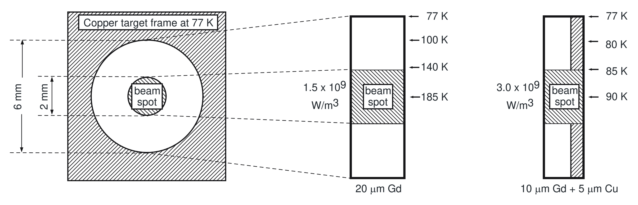
Figure 14: Schematic thermal conductivity calculations. The front view of the target is shown on the left. To the right are shown side views of the targets which indicate the temperature profiles between the center of the target and the point of contact with the target frame. The two cases shown approximate target A in run II (left) and target B in run IV (right).

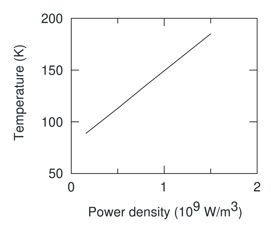
Figure 15: Calculated temperature at the beam spot as a function of beam power-density, $D_{B}$, for a 20 $\mu$m thick gadolinium foil.

Despite the schematic nature of these calculations, and the fact that the foils are rather thin (so bulk thermal conductivities may not apply), the calculations are in very good qualitative agreement with experiment. The two examples shown in Fig. 14 were chosen to resemble target A in run II and target B in run IV. The schematic calculations reproduce the difference in temperature required by the experimental data. Fig 15 shows the linear variation in temperature for a 20 $\mu$m thick gadolinium foil as the beam power is changed. Again, these schematic calculations reproduce the experimental difference between runs II and III.

There remains a difference, of the order of 10%, between the magnetizations of target A and target B under conditions where the beam heating is essentially negligible (runs III and IV). This difference must be attributed to differences in the crystalline texture of the foils.

The thermal conductivity calculations also suggest that even a relatively thin layer of copper evaporated onto a gadolinium foil will greatly assist in keeping the temperature in the beam spot near liquid nitrogen temperature, under conditions where the beam intensity cannot be kept very low. Such a procedure was used for this purpose in Ref. [10].

8 Summary and Conclusions

The effective hyperfine fields experienced by Gd ions recoil-implanted into gadolinium foils have been measured for two targets (one copper-backed) and with differing beam intensities. The effects of (i) the transient-field interaction, (ii) electric-field gradients, and (iii) nuclei residing on damaged, field-free sites have been evaluated. The possible effects of a misalignment between the external field and the direction of the internal magnetization was discussed. It was found that the effective hyperfine magnetic field varies from target to target and with the power deposited by the beam, particularly when the target is an un-backed gadolinium foil.

To a very good approximation, the ratios of hyperfine magnetic fields can be interpreted as ratios of the host magnetization. The changes in hyperfine field strength, and hence magnetization, with beam intensity can be correlated with the expected temperature rise in the beam spot due to the power deposited by the beam. A layer of copper evaporated onto the gadolinium foil can greatly enhance the dissipation of beam power and minimize this temperature rise.

The results of the present measurements were used in a recent study of the transient-fields for high-velocity Ne and Mg ions traversing gadolinium [16], to correct for differences in the magnetizations of the gadolinium foils in targets A and B.

Appendix

In this appendix the formulae are given for calculating perturbed angular correlations in the case where the internal hyperfine fields are misaligned with the external field. Since a full quantitative analysis is not required here, it is necessary to consider the case where only $q=0$ terms are non-zero in Eq. (4). It is then possible to define

$$a_{k}=\sqrt{2k+1}\langle\rho_{k0}\rangle F_{k}Q_{k}.$$ (20)

The case where the internal field is assumed to be distributed equally on a cone of half-angle $\beta$ to the external field has been considered previously by Ben-Zvi et al. [39]. Their expression can be rewritten in the form

$$W(\theta_{\gamma},\beta) = \sum_{kQq}a_{k}[d^{k}_{q0}(\frac{\pi}{2})]^{2}[d^{k}_{Qq}(\beta)]^{2}$$ (21)

$$\times \frac{\cos(q\theta_{\gamma}-Q(\Delta\theta_{Q}+\Delta\theta_{\rm tf}))}{\sqrt{1+Q\omega\tau}}$$

where

$$\tan(Q\Delta\theta_{Q})=Q\omega\tau,$$ (22)

and for convenience in the present application, the spherical harmonics in their expression have been replaced by the $d^{k}_{Qq}(\beta)$ matrices for the second Euler rotation (about the $y$ axis).

To our knowledge, the more general case, where the internal field has a single specific orientation to the external field, specified by the spherical polar co-ordinates $(\beta,\gamma)$ (see Fig. 3), has not been given previously. The result is

$$W(\theta_{\gamma},\beta,\gamma) = \sum_{kQq_{1}q_{2}}a_{k}d^{k}_{q_{1}0}(\frac{\pi}{2})d^{k}_{q_{2}0}(\frac{\pi}{2})d^{k}_{Qq_{1}}(\beta)d^{k}_{Qq_{2}}(\beta)$$ (23)

$$\times \frac{\cos(q_{2}\theta_{\gamma}-(q_{2}-q_{1})\gamma-Q(\Delta\theta_{Q}+\Delta\theta_{\rm tf}))}{\sqrt{1+Q\omega\tau}}.$$

This expression reduces to Eq. (21) when $\gamma$ is averaged between 0 and 2$\pi$ radians:

$$W(\theta_{\gamma},\beta)=\frac{1}{2\pi}\int_{0}^{2\pi}W(\theta_{\gamma},\beta,\gamma)d\gamma$$ (24)

References

- [1] B. Skaali, S. Ogaza, D.G. Fleming and B. Herskind, Phys. Lett. 40 B (1972) 446.
- [2] E.R. Bauminger, A. Diamant, I. Felner, I. Nowik and S. Ofer, Phys. Rev. Lett. 34 (1975) 962.
- [3] R. Kalish, J.L. Eberhardt, K. Dybdal, Phys. Lett. 70 B (1977) 31.
- [4] G.N. Rao, Hyperfine Interact. 7 (1979) 141.
- [5] N. Benczer-Koller, M. Hass, and J. Sak, Annu. Rev. Nucl. Part. Sci. 30 (1980) 53.
- [6] O. Häusser, H.R. Andrews, D. Ward, N. Rud, P. Taras, R. Nicole, J. Keinonen, P. Skensved and C.V. Stager, Nucl. Phys. A 406 (1983) 339.
- [7] O. Häusser, H.R. Andrews, D. Horn, M.A. Lone, P. Taras, P. Skensved, R.M. Diamond, M.A. Deleplanque, E.L. Dines, A.O. Macchiavelli and F.S. Stephens, Nucl. Phys. A 412 (1984) 141.
- [8] R. Vianden, Hyperfine Interact. 35 (1987) 1079.
- [9] A.E. Stuchbery, A.G. White, G.D. Dracoulis, K.J. Schiffer, and B. Fabricius, Z. Phys. A 338 (1991) 135.
- [10] J. Cub, M. Bussas, K.-H. Speidel, W. Karle, U. Knopp, H. Busch, H.-J. Wollersheim, J. Gerl, K. Vetter, C. Ender, F. Köck, J. Gerber, and F. Hagelberg, Z. Phys. A 345 (1993) 1.
- [11] A.E. Stuchbery and S.S. Anderssen, Phys. Rev. C 51 (1995) 1017.
- [12] M.P. Robinson, A.E. Stuchbery, E. Bezakova, S.M. Mullins and H.H. Bolotin, Nucl. Phys. A 647 (1999) 175.
- [13] K.-H. Speidel, O. Kenn, and F. Nowacki, Prog. Part. Nucl. Phys. 49 (2002) 91.
- [14] H.E. Nigh, S. Legvold and F.H. Spedding, Phys. Rev. 132 (1963) 1092.
- [15] M.B. Goldberg, W. Knauer, G.J. Kumbartzki, K.-H. Speidel, J.C. Adloff, and J. Gerber, Hyp. Int. 4 (1978) 262.
- [16] A.E. Stuchbery, A.N. Wilson, P.M. Davidson, A.D. Davies, T.J. Mertzimekis, S.N. Liddick, B.E. Tomlin, P.F. Mantica, Phys. Lett. B 611 (2005) 81.
- [17] C.W. Reich and R.G. Helmer, Nuclear Data Sheets 85 (1998) 171.
- [18] C.W. Reich, Nuclear Data Sheets 104 (2005) 1.
- [19] C.W. Reich, Nuclear Data Sheets 99 (2003) 753.
- [20] R.G. Helmer, Nuclear Data Sheets 103 (2004) 565.
- [21] R.G. Helmer, Nuclear Data Sheets 101 (2004) 325.
- [22] C.W. Reich, Nuclear Data Sheets 78 (1996) 547.
- [23] S. Raman, C.W. Nestor, Jr., and P. Tikkanen, Atom. Data Nucl. Data Tables 78, 1 (2001).
- [24] A.E. Stuchbery, Nucl. Phys. A 589 (1995) 222.
- [25] D.B. Laubacher, Y. Tanaka, R.M. Steffen, E.B. Shera and M.V. Hoehn, Phys. Rev. C 27 (1983) 1772.
- [26] A. Piqué, J.M. Brennan, R. Darling, R. Tanczyn, D. Ballon and N. Benczer-Koller, Nucl. Inst. Meth. A 279 (1989) 579.
- [27] C.S. Barrett and T.B. Massalski, Structure of metals: crystallographic Methods, principles, and Data, McGraw-Hill, New York, 3rd Edition, 1966.
- [28] W.D. Hutchison, private communication.
- [29] A.E. Stuchbery and M.P. Robinson, Nucl. Instrum. Methods A 485 (2002) 753.
- [30] K. Alder and A. Winther, Electromagnetic Excitation, North Holland, Amsterdam, 1975.
- [31] A. Winther and J. de Boer, Coulomb Excitation, eds. K. Alder and A. Winther (Academic Press, New York, 1966) p. 303.
- [32] T. Yamazaki, Nuclear Data A3 (1967) 1.
- [33] K. Alder, E. Matthias, W. Schneider and R.M. Steffen, Phys. Rev. 129 (1963) 1199.
- [34] E. Matthias, W. Schneider and R.M. Steffen, Phys. Rev. 125 (1962) 261.
- [35] A.E. Stuchbery, S.S. Anderssen and E. Bezokova, Hyperfine Interact. 97/98 (1996) 479.
- [36] N.K.B. Shu, D. Melnik, J.M. Brennan, W. Semmler and N. Benczer-Koller, Phys. Rev. C 21 (1980) 1828.
- [37] A.E. Stuchbery and E. Bezakova, Australian Journal Physics 51 (1998) 183.
- [38] QuickField software, Tera Analysis Ltd., http://www.quickfield.com.
- [39] I. Ben-Zvi, P. Gilad, G. Goldring, P. Hillman, A. Schwarzschild and Z. Vager, Phys. Rev. Lett. 19 (1967) 373.