Branching Ratios for the Beta Decay of ²¹Na

Abstract

We have measured the beta-decay branching ratio for the transition from ²¹Na to the first excited state of ²¹Ne. A recently published test of the standard model, which was based on a measurement of the $\beta$-$\nu$ correlation in the decay of ²¹Na, depended on this branching ratio. However, until now only relatively imprecise (and, in some cases, contradictory) values existed for it. Our new result, $4.74(4)\%$, reduces but does not remove the reported discrepancy with the standard model.

I Introduction

A recent publication by Scielzo et al.Sc04 reported a measurement of the $\beta$-$\nu$ angular correlation coefficient, $a_{\beta\nu}$, for the $\beta$-decay transition between ²¹Na and the ground state of its mirror, ²¹Ne. The authors compare their result with the standard-model prediction for $a_{\beta\nu}$, with a view to testing for scalar or tensor currents, the presence of which would signal the need for an extension of the standard model. Although they found a significant discrepancy – the measured value, $a_{\beta\nu}=0.524(9)$, disagrees with the standard-model prediction of 0.558 – they stop short of claiming a fundamental disagreement with the standard model.

Scielzo et al. Sc04 offer two alternative explanations that would have to be eliminated before their result could begin to raise questions about the need for an extension to the standard model. One is that some ²¹Na₂ dimers formed by cold photoassociation could also have been present in their trap, thus distorting the result; they themselves propose to do further measurements to test that possibility. The other is that the branching-ratio value they used for $\beta$ decay to the first excited state of ²¹Ne might not be correct. Because Scielzo’s measurement could not distinguish between positrons from the two predominant $\beta$-decay branches from ²¹Na (see Fig. 1), the adopted branching ratio for the $\beta$ transition to the first excited state not only affects their data analysis but also helps determine the theoretical prediction for $a_{\beta\nu}$ itself, since the axial-vector component of the ground-state branch can only be determined from its $ft$ value, which also depends on the branching ratio. This branching ratio is a key component of their standard-model test, yet the five published values Ta60 ; Ar63 ; Al74 ; Az77 ; Wi80 are between 25 and 45 years old, are quite inconsistent with one another and range from 2.2(3) to 5.1(2)%. To remedy this problem, we report here a new measurement of the ground-state branching ratio, for which we quote $\pm$0.8% relative precision, five times better than the best precision claimed in any previous measurement.

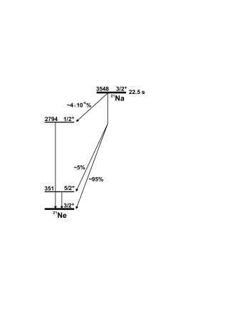
Figure 1: $\beta$-decay scheme for ²¹Na

II Experiment

We produced 22.5-s ²¹Na using a 28A-MeV ²²Ne beam from the Texas A&M K500 superconducting cyclotron to initiate the ¹H(²²Ne, $2n$)²¹Na reaction on a LN₂-cooled hydrogen gas target. The ejectiles from the reaction were fully stripped and, after passing through the MARS spectrometer Tr91 , produced a ²¹Na secondary beam of $>$99% purity at the extraction slits in the MARS focal plane. This beam, containing $\sim$$3\times 10^{5}$ atoms/s at $24.4A$ MeV, then exited the vacuum system through a 50-$\mu$m-thick Kapton window, passed successively through a 0.3-mm-thick BC-404 scintillator and a stack of aluminum degraders, finally stopping in the 76-$\mu$m-thick aluminized mylar tape of a tape transport system. Since the few impurities remaining in the beam had ranges different from that of ²¹Na, most were not collected on the tape; residual collected impurities were concluded to be less than $0.1$% of the ²¹Na content.

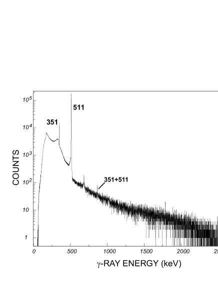
Figure 2: Spectrum of $\beta$-delayed $\gamma$ rays observed in coincidence with positrons following the decay of ²¹Na. It includes about half of the total data collected. The peaks attributable to ²¹Na are marked with their energy in keV; the sum peak is identified by its components. The small unmarked peak at 682 keV is caused by summing of one 511-keV $\gamma$ ray with the back-scattered $\gamma$ ray (171 keV) from the second 511-keV $\gamma$ ray.

In a typical measurement, we collected ²¹Na on the tape for a few seconds, then interrupted the beam and triggered the tape-transport system to move the sample in 180 ms to a shielded counting station located 90 cm away, where the sample was positioned between a 1-mm-thick BC404 scintillator to detect $\beta^{+}$ particles, and a 70% HPGe detector for $\gamma$ rays. Two timing modes were used: in one, the collection and detection periods were 3 and 30 s, respectively; in the other, they were 6 and 60 s. In both cases, after the detection period was complete, the cycle was repeated and, in all, some 3,200 cycles were completed over a span of 32 hours.

Time-tagged $\beta$-$\gamma$ coincidence data were stored event by event. The $\beta$ and $\gamma$-ray energies, the coincidence time between them, and the time of the event after the beginning of the cycle were all recorded, as was the total number of $\beta$-singles events for each cycle. The same discriminator signal used for scaling was also used in establishing the $\beta$-$\gamma$ coincidences.

Essential to our experimental method is the precise absolute efficiency of the $\gamma$-ray detector, which was positioned 15 cm from the collected sample. We have meticulously calibrated our HPGe detector at this distance over a five-year period using, in total, 13 individual sources from 10 different radionuclides: ⁴⁸Cr, ⁶⁰Co, ⁸⁸Y, ^108mAg, ¹⁰⁹Cd, ^120mSb, ¹³³Ba, ¹³⁴Cs, ¹³⁷Cs and ^180mHf. Two of the ⁶⁰Co sources were specially prepared by the Physikalisch-Technische Bundesanstalt Sc02 with activities certified to 0.06%. The details of our calibration procedures, which include both source measurements and Monte Carlo calculations, have been published elsewhere Ha02 ; He03 ; He04 . The absolute efficiency of our detector is known to 0.2% in the energy range from 50 to 1400 keV, and to 0.4% from 1400 keV to 3.5 MeV.

The absolute efficiency of the $\beta^{+}$ detector, which was located 1.5 cm from the collected sample, is not required for our measurement but its dependence on energy is of some importance (see section III). We have explored the efficiency of this detector via measurements and Monte Carlo calculations, and its dependence on $\beta^{+}$ energy is now reasonably well understood Ia06 .

A typical $\gamma$-ray spectrum recorded in coincidence with betas is presented in Fig. 2. Apart from the annihilation radiation, the only significant peak in the spectrum is the 351-keV $\gamma$ ray from the first excited state in ²¹Ne. In 3,200 total cycles we recorded more than $8\times 10^{4}$ counts in this peak.

It was important to our later analysis that we establish the contribution of room background both to the $\beta$-$\gamma$ coincidence spectrum and to the $\beta$-detector singles rate. For this purpose, we recorded data with the cyclotron beam on but with a thick degrader inserted just upstream from the tape; everything was thus identical to a normal measurement except that no ²¹Na was implanted in the tape. Both the coincidence and singles rates were observed to drop to 0.04% of the rate observed when ²¹Na was correctly implanted. Room background was thus effectively negligible in our analysis.

III Results

The $\beta$-decay scheme of ²¹Na is shown in Fig. 1. The only branch in addition to those populating the ground and first excited states is known to be very weak Wi80 and can be ignored in our analysis. In that case, the branching ratio, $R_{1}$, for population of the first excited state can be determined from the measured intensity ratio of the 351-keV $\gamma$ ray relative to the total number of ²¹Na decays. Thus, we obtain $R_{1}$ from the following relationship:

$$R_{1}=\frac{N_{\gamma\beta}}{N_{\beta}\epsilon_{\gamma}}k,$$ (1)

where $N_{\gamma\beta}$ is the number of 351-keV $\gamma$ rays observed in coincidence with betas; $N_{\beta}$ is the number of (singles) betas observed; $\epsilon_{\gamma}$ is the efficiency of the HPGe detector for 351-keV $\gamma$ rays; and $k$ is a factor ($\sim$ 1) that accounts for small experimental corrections that will be enumerated in what follows. Note that the efficiency of the beta detector does not appear in Eq. 1, although its dependence on $\beta^{+}$ energy will be seen to play a minor role in the evaluation of $k$.

Before determining the ratio $N_{\gamma\beta}/N_{\beta}$ from our data, we eliminated those cycles in which the collected source was not positioned exactly between the $\beta$ and $\gamma$ detectors. Although the tape-transport system is quite consistent in placing the collected source within $\pm 3$ mm of the designated counting location, it is a mechanical system, and occasionally larger deviations occur. For each cycle we recorded not only the total number of positrons detected but also the total number of ²¹Na ions that emerged from the MARS spectrometer, as detected by the scintillator located immediately in front of the aluminum degraders. The ratio of the former to the latter is a very sensitive measure of how well the source is positioned with respect to the $\beta$ detector. In analyzing the data, we rejected the results from any cycle with an anomalous (low) ratio. Under these conditions, we obtained the result $N_{\gamma\beta}/N_{\beta}=2.378(13)\times 10^{-4}$.

As stated in section II, the absolute efficiency, $\epsilon_{\gamma}$, of our detector at 15 cm is known to $\pm 0.2\%$. However, this applies to a highly controlled situation in which the source-to-detector distance can be measured by micrometer to a small fraction of a millimeter. With the fast tape-transport delivery system, we cannot be assured of reproducibility at the same level of precision. Taking $\pm 0.5$ mm to be our actual uncertainty in position under experimental conditions, we add an uncertainty of $\pm 0.6\%$ to the detector efficiency in quadrature with the basic $\pm 0.2\%$ uncertainty. For the 351-keV $\gamma$ ray, this leads to $\epsilon_{\gamma}=5.12(3)\times 10^{-3}$, the value we insert in Eq. 1.

Although the ratio $N_{\gamma\beta}/N_{\beta}$ and $\epsilon_{\gamma}$ are the predominant experimental quantities required to evaluate the branching ratio, it is the correction factor $k$ that holds the key to our achieving high precision. In fact, $k$ is really a product of four separate corrections, $k_{1}...k_{4}$. We will deal with each individually.

Random coincidences $(k_{1})$. — Since the time between each coincident $\beta$ and $\gamma$ ray was recorded event by event, we could project out the time spectrum corresponding to the 351-keV $\gamma$ ray. In that spectrum, the prompt coincidence peak stood prominently above the flat random distribution, allowing us clearly to distinguish the relative contributions of real and random coincidences. The correction factor required to account for the random contribution to the $\beta$-coincident 351-keV $\gamma$-ray peak was thus determined to be $k_{1}$ = 0.9884(10). Naturally, this correction accounts not only for random coincidences among ²¹Na $\beta$ and $\gamma$ rays but also for random coincidences between ²¹Na betas and any $\gamma$ rays originating from room background.

Real-coincidence summing $(k_{2})$.— Since each 351-keV $\gamma$ ray from the decay of the first excited state in ²¹Ne is accompanied by a positron from the ²¹Na $\beta^{+}$-decay branch that populated the state, there is a significant probability that a 351-keV $\gamma$ ray and 511-keV annihilation radiation will reach our HPGe detector simultaneously and be recorded as a single $\gamma$ ray with the combined energy of both. Any summing of this kind will rob events from the 351-keV photopeak. Our first step in accounting for the resultant loss was to obtain the area of the observed 862-keV (511+351) sum peak. Since losses from the 351-keV photopeak result not just from its summing with the 511-keV photopeak but also with the latter’s Compton scattered radiation, as a second step we multiplied the sum-peak area by the known “total-to-peak” ratio for our detector at 511 keV (see Fig. 11 in reference He03 ). Finally, this result for losses was increased by 4% to account for annihilation in flight, which leads to 351-keV peak summing with annihilation radiation of different energies, and by another 2.5% to account for summing with positrons backscattered from the plastic scintillator. The total loss due to real-coincidence summing was thus determined to be 1.78%: i.e. $k_{2}$ = 1.0178(17).

Dead time $(k_{3})$.— Equation 1 depends upon $N_{\gamma\beta}$ and $N_{\beta}$ being recorded for identical times. In our experiment they were, of course, gated on and off together, but during the counting period the circuit dead time for $N_{\gamma\beta}$, which was limited by the relatively slow electronics used for $\gamma$-ray counting, was much greater than that for $N_{\beta}$, which was simply scaled. We determined the dead time associated with $N_{\gamma\beta}$ from the total rate in the HPGe detector during the counting period and from the known processing time (32 $\mu$s) for each coincident event. The scaler dead time per event was only 100 ns but the total rate in the scaler was much higher than the HPGe rate; nevertheless the dead time associated with $N_{\beta}$ turned out to be smaller by a factor of three than that associated with coincidence events. The overall correction factor is $k_{3}$ = 1.0018(1).

Table 1: Error budget for the measured branching ratio $R_{1}$

Origin of uncertainty	$\%$ uncertainty
Experimental ratio, $N_{\gamma\beta}/N_{\beta}$	0.52
HPGe detector efficiency	0.20
Source-detector distance	0.60
Random coincidences	0.11
Real-coincidence summing	0.17
Dead time	0.01
$\beta$-detector efficiency vs energy	0.13
Total uncertainty on $R_{1}$	0.85

Beta-detector response function $(k_{4})$.— The correction factor associated with the $\beta$-detector response function is given by

$$k_{4}=\frac{\epsilon_{\beta_{total}}}{\epsilon_{\beta_{1}}}\simeq\frac{0.95\epsilon_{\beta_{0}}+0.05\epsilon_{\beta_{1}}}{\epsilon_{\beta_{1}}},$$ (2)

where $\epsilon_{\beta_{0}}$ and $\epsilon_{\beta_{1}}$ are the detector efficiencies for the $\beta$ transitions to the ground and first excited states respectively. If the detector response function were completely independent of energy, then this correction factor would be unity. In fact, though, the efficiency does change slightly with energy. We have studied this effect using measurements with sources – ⁹⁰Sr, ¹³³Ba, ¹³⁷Cs and ²⁰⁷Bi – aided by Monte Carlo calculations Ia06 . Including the effects of our low-energy electronic threshold, we determine that $\epsilon_{\beta_{1}}/\epsilon_{\beta_{0}}$ = 0.987, which leads to the correction factor $k_{4}$ = 1.0129(13).

Multiplying $k_{1}$ through $k_{4}$ we determine the correction factor in Eq. 1 to be $k$ = 1.0208(24). When combined in Eq. 1 with the other factors already discussed, this yields the final result for the branching ratio to the first excited state in ²¹Na:

$$R_{1}=0.0474(4).$$ (3)

The complete error budget corresponding to our quoted $\pm 0.85\%$ uncertainty is given in Table 1.

IV Analysis

Our measured branching-ratio value is compared with previous measurements in Table 2. All previous experiments determined the branching ratio from a comparison of the area of the 351-keV peak to that of the annihilation radiation. This method has the advantage that only relative detector efficiencies are required, but it has three serious disadvantages: i) contaminant activities may well make an unknown contribution to the annihilation radiation; ii) most positrons do not annihilate at the source position, where the $\gamma$ rays originate, so the relative detection efficiencies cannot be simply determined from calibration sources; and iii) the significant effect ($\sim$5%) of positron annihilation in flight is a first-order correction that must be calculated and corrected for. All previous measurements except possibly reference Al74 were susceptible to potential contaminants; only the last three references Al74 ; Az77 ; Wi80 mention accounting for a spatially distributed source of 511-keV radiation; and only the last two Az77 ; Wi80 appear to have taken account of annihilation in flight.

Table 2: Measurements of the branching ratio $R_{1}$

Date	Reference	Result(%)
1960	Talbert & Stewart Ta60	2.2(3)
1963	Arnell & Wernbom Ar63	2.3(2)
1974	Alburger Al74	5.1(2)
1977	Azuelos, Kitching & Ramavataram Az77	4.2(2)
1980	Wilson, Kavanagh & Mann Wi80	4.97(16)
2006	This measurement	4.74(4)

Given the age of the previous measurements and the potential hazards associated with their experimental method – not to mention their mutual inconsistency – we choose not to average our result with them but instead to use our present result alone in extracting the properties of the ²¹Na $\beta$-decay scheme.

Since there are only two significant $\beta$-decay branches from ²¹Na – to the ground and first excited states of the daughter – with $R_{1}$ determined, the branching ratio to the ground state, $R_{0}$, follows directly from it:

$$R_{0}=0.9526(4),$$ (4)

where this result is actually determined to a precision of 0.04%. We now proceed from this value for $R_{0}$ to obtain the $ft$ value for this transition, the relative contributions of axial-vector and vector components, and ultimately the standard-model expectation for its $\beta$-$\nu$ angular correlation coefficient.

In deriving the $ft$ value for the ground-state mirror transition, we take the half-life of ²¹Na to be $t_{1/2}$ = 22.49(4) s and its total decay energy to be $Q_{EC}$ = 3547.6(7) keV. The former is the average of two mutually consistent results Al74 ; Az77 and the latter is the value quoted in the 2003 Atomic Mass Evaluation Au03 where it was obtained from a single ²⁰Ne(p,$\gamma$)²¹Na measurement made in 1969 Bl69 and then revised by Audi et al. Au03 to take account of more up-to-date calibration energies. With the calculated electron-capture probability for the ground-state transition being 0.00095, the average half life, when combined with our branching ratio value from Eq. 4, yields a partial half-life for the transition of 23.63(4) s.

Next we compute the value of $f$ from the $Q_{EC}$ value following methods similar to those we used in the analysis of superallowed $\beta$ decay; these are described in the Appendix to reference Ha05 . To make an “exact” calculation that includes, for example, the effects of weak magnetism and other induced corrections we need a shell-model calculation of the appropriate nuclear matrix elements. For this we used an $(s,d)$-shell model space and the universal $(s,d)$-shell effective interaction of Wildenthal Wi84 . This interaction has been demonstrated Br85 to reproduce energy spectra and Gamow-Teller matrix elements in this mass region providing that the axial-vector coupling constant is quenched. In our calculation, we fine-tuned the amount of quenching to reproduce our experimental data.

For a mirror transition like this one, which includes both vector and axial-vector components, the $f$ value calculated for the vector part of the weak interaction, $f_{\mbox{\tiny V}}$, is slightly different from the value calculated for the axial-vector part, $f_{\mbox{\tiny A}}$. In the allowed approximation it is always assumed that $f_{\mbox{\tiny V}}$ = $f_{\mbox{\tiny A}}$ = $f$ but, where high precision is sought, a more exact calculation is required. The results we obtain, $f_{\mbox{\tiny V}}$ = 170.974 and $f_{\mbox{\tiny A}}$ = 174.157, are nearly 2% different from one another, principally as a result of the influence of weak magnetism on the shape correction factor of the axial-vector component. In quoting the $ft$ value for the mirror ground-state transition, we make the (arbitrary) choice to use $f_{\mbox{\tiny V}}$, with the result that

$$f_{\mbox{\tiny V}}t=4040(9)s.$$ (5)

Like any other $ft$ value, this result can be related to vector and axial-vector coupling constants, and to the matrix elements pertaining to the specific transition. To do so with the precision required for a standard-model test requires that radiative and charge-dependent corrections be incorporated. The expression we use is the following:

$$\Bigm{[}f_{\mbox{\tiny V}}G_{\mbox{\tiny V}}^{2}\langle 1\rangle^{2}(1+\delta_{NS}-\delta_{C})(1+\Delta_{\mbox{\tiny R}}^{\mbox{\tiny V}})~{}~{}~{}~{}~{}~{}~{}~{}~{}~{}~{}$$

$$+f_{\mbox{\tiny A}}G_{\mbox{\tiny A}}^{2}\langle\sigma\rangle^{2}(1-\delta_{A})(1+\Delta_{\mbox{\tiny R}}^{\mbox{\tiny A}})\Bigm{]}(1+\delta_{R}^{\prime})t = K~{}~{}~{}~{}~{}~{}~{}~{}$$ (6)

where $K/(\hbar c)^{6}=(8120.271\pm 0.012)\times 10^{-10}$ GeV^-4s; $G_{\mbox{\tiny V}}$ and $G_{\mbox{\tiny A}}$ are the vector and axial-vector coupling constants for nuclear weak decay; and $\langle 1\rangle$ and $\langle\sigma\rangle$ are the Fermi (vector) and Gamow-Teller (axial-vector) matrix elements, respectively, for the ground-state transition. For this particular transition between T=$\frac{1}{2}$ states, $\langle 1\rangle$=1. The transition-dependent radiative correction terms, $\delta_{R}^{\prime}$ and $\delta_{NS}$, and the isospin-symmetry-breaking correction, $\delta_{C}$, all have their conventional definitions Ha05 but, in the present context of a mixed vector and axial-vector transition, we note that $\delta_{R}^{\prime}$ is the same for both components while $\delta_{C}$ and $\delta_{NS}$ only pertain to the vector component. The latter two terms have their equivalents that must be applied to the axial-vector component but we subsume them into a term we call $\delta_{A}$: as it turns out, we will not have to calculate a value for $\delta_{A}$. Finally, the transition-independent radiative correction also takes on different values for the vector and axial-vector components, $\Delta_{\mbox{\tiny R}}^{\mbox{\tiny V}}$ and $\Delta_{\mbox{\tiny R}}^{\mbox{\tiny A}}$; but neither will have to be calculated.

Rearranging Eq. 6, we obtain the result:

$$f_{\mbox{\tiny V}}t(1+\delta_{R}^{\prime})(1+\delta_{NS}-\delta_{C})=\frac{K}{G_{\mbox{\tiny V}}^{2}(1+\Delta_{\mbox{\tiny R}}^{\mbox{\tiny V}})\bigm{[}1+\lambda^{2}\frac{f_{\mbox{\tiny A}}}{f_{\mbox{\tiny V}}}\bigm{]}}$$ (7)

where

$$\lambda=\frac{G_{\mbox{\tiny A}}\langle\sigma\rangle(1-\delta_{A})^{1/2}(1+\Delta_{\mbox{\tiny R}}^{\mbox{\tiny A}})^{1/2}}{G_{\mbox{\tiny V}}(1+\delta_{NS}-\delta_{C})^{1/2}(1+\Delta_{\mbox{\tiny R}}^{\mbox{\tiny V}})^{1/2}}.$$

Here $\lambda$ is the ratio of axial-vector to vector components in the transition. A further simplification in this equation can be achieved by our implementing the results from superallowed $0^{+}\rightarrow 0^{+}$ beta decays, which provide an experimental determination of the product $G_{\mbox{\tiny V}}^{2}(1+\Delta_{\mbox{\tiny R}}^{\mbox{\tiny V}})$. The average corrected ${{\cal F}t}$ value from these decays Ha05 is related to the vector coupling constant via the relationship:

$$\overline{{\cal F}t}=\frac{K}{2G_{\mbox{\tiny V}}^{2}(1+\Delta_{\mbox{\tiny R}}^{\mbox{\tiny V}})}.$$ (8)

Since it is the term $\lambda$ that we need to extract from experiment in order to calculate the $\beta$-$\nu$ angular correlation coefficient, we now re-express Eq. 7 in the following form:

$$\lambda^{2}=\frac{f_{\mbox{\tiny V}}}{f_{\mbox{\tiny A}}}\Bigm{[}\frac{2\overline{{\cal F}t}}{f_{\mbox{\tiny V}}t(1+\delta_{R}^{\prime})(1+\delta_{NS}-\delta_{C})}-1\Bigm{]}.$$ (9)

We have calculated the three remaining correction terms using the same methods as were described in reference To02 , the results being $\delta_{R}^{\prime}$ = 1.492(15)%, $\delta_{C}$ = 0.268(16)% and $\delta_{NS}$ = -0.065(20)%. We then adopt the value, $\overline{{\cal F}t}$ = 3072.7(8), which is the average result extracted from superallowed $0^{+}\rightarrow 0^{+}$ beta decays when the correction terms are calculated by the same methods as those used here (see Eq. 11 in reference Ha05 ). Thus we finally obtain

$$\lambda=0.7033(24)$$ (10)

for the ground-state mirror transition.

Based on this result for $\lambda$ we have computed the beta-neutrino correlation coefficient exactly, following the formalism of Behrens-Bühring Be82 . These authors write the electron-neutrino correlation $\omega(\theta,W)$ as:

$$\omega(\theta,W)=\sum_{k}D(k,W)P_{k}(\cos\theta),$$ (11)

where $W$ is the electron energy (in rest-mass units), $\theta$ is the angle between the emitted electron and neutrino directions, and $P_{k}$ are Legendre polynomials. The sum is over $k=0,1,2$. The coefficients $D(k,W)$ are expressed fully by Behrens and Bühring Be82 , from which it can be seen that $D(0,W)$ is exactly equal to 1.0, and $D(2,W)$ is small. The term $D(1,W)$ relates to the beta-neutrino angular correlation coefficient, $a_{\beta\nu}$, via the expression

$$D(1,W)=a_{\beta\nu}p/W,$$ (12)

where $p=\sqrt{W^{2}-1}$. For the exact expression for $a_{\beta\nu}$ we compute

$$a_{\beta\nu}=\langle D(1,W)W/p\rangle,$$ (13)

where $\langle..\rangle$ signifies an average over the beta spectrum. It should be noted that this exact evaluation of $a_{\beta\nu}$ yields a result that is about 1% different from the approximate expression that is often used: viz.

$$(a_{\beta\nu})_{approx}=(1-\lambda^{2}/3)/(1+\lambda^{2}).$$ (14)

The exact expression in Eq. 13 differs from this approximate one by the inclusion of energy dependence as well as weak magnetism and other small effects. Our final computed result for the exact $\beta$-$\nu$ angular correlation coefficient based on our new experimental result for $\lambda$ is

$$a_{\beta\nu}=0.553(2).$$ (15)

This can now stand as the “standard-model prediction” for $a_{\beta\nu}$, against which the measured angular-correlation coefficient can be compared. Our new value is 0.9% lower than the one originally used by Scielzo et al. Sc04 .

V Conclusions

As noted in the Introduction, the value of the branching ratio affects not only the standard-model prediction for $a_{\beta\nu}$ (see Eq. 15) but also the analysis by Scielzo et al. Sc04 of their measurement of that coefficient. With the excited-state branching ratio taken to be 5.02(13)%, they applied a correction of +6.81(18)% to their result. Since this correction scales with the branching ratio Sc05 , our new value for the latter leads to a new correction factor of +6.44(5)%. This downward shift of 0.4% is actually rather small compared to the overall uncertainties quoted by Scielzo et al., and their value for $a_{\beta\nu}$ as obtained from ²¹Ne¹⁺ only changes from 0.524(9) to 0.523(9).

As a result of our new measurement we have improved – and lowered slightly – the standard-model prediction of the $\beta$-$\nu$ angular correlation coefficient for the mirror transition from ²¹Na. This new prediction still leaves the Scielzo et al. experimental result Sc04 in disagreement with the prediction. However, the authors themselves expressed concern about the possible presence of ²¹Na₂ dimers in their trapped samples; this would have caused a dependence of their result on the trapped-atom population and could easily reconcile their result with the standard model. With a precise branching ratio now determined, an investigation of the actual make-up of the trapped-atom samples in the Scielzo et al. experiment is essential if the ²¹Na result is to become a real test of the standard model.

Finally, we draw attention to the fact that the “standard-model prediction” for $a_{\beta\nu}$ depends on the half-life of ²¹Na and its $\beta$-decay $Q$ value through the $f_{\mbox{\tiny V}}t$ value for the ground-state transition (see Eq. 5 and the preceeding paragraphs). The half-life has only been measured twice Al74 ; Az77 – in experiments that did not obtain branching ratios in agreement with our current result – and the $Q$ value comes from a single 35-year-old (p,$\gamma$) measurement Bl69 originally based on long-outdated calibration energies. Clearly, both these results could be improved significantly by modern measurements.

The authors would like to thank N.D. Scielzo for helpful discussions. This work was supported by the U.S. Department of Energy under Grant No. DE-FG03-93ER40773 and by the Robert A. Welch Foundation under Grant No. A-1397.

References

- (1) N.D. Scielzo, S.J. Freedman, B.K. Fujikawa and P.A. Vetter, Phys. Rev. Lett. 93, 102501 (2004).
- (2) W.L. Talbert, Jr. and M.G. Stewart, Phys. Rev. 119, 272 (1960).
- (3) S.E. Arnell and E. Wernbom, Arkiv für Fysik 25, 389 (1963).
- (4) D.E. Alburger, Phys. Rev. C 9, 991 (1974).
- (5) G. Azuelos, J.E. Kitching and K. Ramavataram, Phys. Rev. C 15, 1847 (1977).
- (6) H.S. Wilson, R.W. Kavanagh and F.M. Mann, Phys. Rev. C 22, 1696 (1980).
- (7) R.E. Tribble, C.A. Gagliardi and W. Liu, Nucl. Instrum. Methods Phys. Res., Sect. B 56/57, 956 (1991).
- (8) E. Schönfeld, H. Janssen, R. Klein, J.C. Hardy, V.E. Iacob, M. Sanchez-Vega, H.C. Griffin, M.A. Luddington, Int. J. Appl. Radiat. Isot. 56, 215 (2002).
- (9) J.C. Hardy, V.E. Iacob, M. Sanchez-Vega, R.T. Effinger, P. Lipnik, V.E. Mayes, D.K. Willis, R.G. Helmer, Int. J. Appl. Radiat. Isot. 56, 65 (2002).
- (10) R.G. Helmer, J.C. Hardy, V.E. Iacob, M. Sanchez-Vega, R.G. Neilson, J. Nelson, Nucl. Instrum. Methods Phys. Res., Sect. A 511, 360 (2003).
- (11) R.G. Helmer, N. Nica, J.C. Hardy, V.E. Iacob, Int. J. Appl. Radiat. Isot. 60, 173 (2004).
- (12) V.E. Iacob et al., to be published.
- (13) G. Audi, A.H. Wapstra and C. Thibault, Nucl. Phys. A 729, 337 (2003).
- (14) R. Bloch, T. Knellwolf and R.E. Pixley, Nucl. Phys. A 123, 129 (1969).
- (15) J.C. Hardy and I.S. Towner, Phys. Rev. C 71, 055501 (2005).
- (16) B.H. Wildenthal, Prog. in Part. and Nucl. Phys. 11, 5 (1984).
- (17) B.A. Brown and B.H. Wildenthal, At. Data Nucl. Data Tables 33, 347 (1985).
- (18) I.S. Towner and J.C. Hardy, Phys. Rev. C 66, 035501 (2002).
- (19) H. Behrens and W. Bühring, Electron Radial Wave Functions and Nuclear Beta-decay (Clarendon Press, Oxford, 1982).
- (20) N. Scielzo, private communication (2005).