A Method for Measuring Elliptic Flow Fluctuations in PHOBOS

Abstract

We introduce an analysis method to measure elliptic flow $(v_{2})$ fluctuations using the PHOBOS detector for Au+Au collisions at $\sqrt{s_{NN}}=200$ GeV. In this method, $v_{2}$ is determined event-by-event by a maximum likelihood fit. The non-statistical fluctuations are determined by unfolding the contribution of statistical fluctuations and detector effects using Monte Carlo simulations(MC). Application of this method to measure dynamical fluctuations embedded in special MC are presented. It is shown that the input fluctuations are reconstructed successfully for $\langle v_{2}\rangle\geq 0.03$.

I Introduction

Studies of collective flow have proven to be fruitful probes of the dynamics of heavy ion collisions. Elliptic flow $(v_{2})$ in heavy ion collisions was first discussed in FirstFlowPaper and has been measured at AGSAGS1 ; AGS2 and SPSSPS1 ; SP2 energies. The first measurement of elliptic flow at RHIC was performed by the STAR collaborationStar1 . PHOBOS has measured elliptic flow as a function of pseudorapidity, centrality, transverse momentum, center-of-mass energy and nuclear speciesPhobosFlowPRL1 ; PhobosFlowPRL2 ; PhobosFlowPRC ; ManlyQM . In particular, the measurements of $v_{2}$ as a function of centrality provide information on how the azimuthal anisotropy of the initial collision region drives the azimuthal anisotropy in particle production. When two nuclei collide with non-zero impact parameter, the almond-shaped overlap region has an azimuthal spatial asymmetry. If the particles do not interact after their initial production, the asymmetrical shape of the source region will have no impact on the azimuthal distribution of detected particles. Therefore, observation of azimuthal asymmetry in the outgoing particles is direct evidence of interactions between the produced particles. In addition, the interactions must have occurred at relatively early times, since expansion of the source, even if uniform, will gradually erase the magnitude of the spatial asymmetry. Hydrodynamical models can be used to calculate a quantitative relationship between a specific initial source shape and the distribution of emitted particlesHydroRef1 . At the high RHIC energies, the elliptic flow signal at midrapidity in Au+Au collisions is as large as that calculated under the assumption of a boost-invariant relativistic hydrodynamic fluid. The presence of a large flow signal has been considered to be a proof of early equilibration in the colliding systemWhitePaper .

The azimuthal anisotropy of the initial collision region is quantified by the eccentricity of the overlap region of the colliding nuclei. The customary definition of eccentricity, which we call the “standard eccentricity,” is determined by relating the impact parameter of the collision in a Glauber model simulation to the eccentricity calculated assuming the minor axis of the overlap ellipse to be along the impact parameter vector. Thus, if the $x$ axis is defined to be along the impact parameter vector and the $y$ axis perpendicular to that in the transverse plane, the eccentricity is defined by:

$$\epsilon_{standard}=\frac{\sigma_{y}^{2}-\sigma_{x}^{2}}{\sigma_{y}^{2}+\sigma_{x}^{2}},$$ (1)

where $\sigma_{x}$ and $\sigma_{y}$ are the RMS widths of the participant nucleon distributions projected on the $x$ and $y$ axes, respectively.

Measurement of $v_{2}$ fluctuations as a probe of early stage dynamics of heavy-ion collisions has been suggested earlier by Mrowczynski and ShuryakShuryak . However, Miller and Snellings have pointed out that fluctuations in the shape of the initial collision region must be understood first before addressing other physical sources of $v_{2}$ fluctuationsSnellings . Furthermore, the latter argue that experimental measurements of $v_{2}$ can be affected by these fluctuations. They show approximate agreement between the predictions from a fluctuating eccentricity model and the differences in $v_{2}$ measures obtained via two, four and six particle cumulant methods in Au+Au collisions, where the standard definition of eccentricity is used.

The elliptic flow in Cu+Cu collisions is observed to be surprisingly large, particularly for the most central eventsManlyQM . PHOBOS has proposed that event-by-event fluctuations in the shape of the initial collision region can be a possible explanation for the large $v_{2}$ signal in the small Cu+Cu systemManlyQM . For small systems or small transverse overlap regions, fluctuations in the nucleon positions frequently create a situation where the minor axis of the ellipse in the transverse plane formed by the participating nucleons is not along the impact parameter vector. An alternative definition of eccentricity, called the “participant eccentricity”, $\epsilon_{part}$, is introduced to account for the nucleon position fluctuations such that the eccentricity is calculated with respect to the minor axis of the ellipse defined by the distribution of participants found using a Monte Carlo approach. Using the same coordinates as before:

$$\epsilon_{part}=\frac{\sqrt{(\sigma_{y}^{2}-\sigma_{x}^{2})^{2}+4\sigma_{xy}^{2}}}{\sigma_{y}^{2}+\sigma_{x}^{2}},$$ (2)

where $\sigma_{xy}=\langle xy\rangle-\langle x\rangle\langle y\rangle$. The average values of $\epsilon_{standard}$ and $\epsilon_{part}$ are quite similar for all but the most peripheral interactions for the Au+Au system. For the smaller Cu+Cu system, however, fluctuations in the nucleon positions become quite important for all centralities and the average eccentricity can vary significantly depending on how it is calculatedManlyQM .

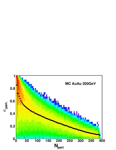
Figure 1: Participant eccentricity, $\epsilon_{part}$, of the collision zone as a function of number of partipicant nucleons, $N_{part}$, for Au+Au collisions at $\sqrt{s_{NN}}=200$ GeV from the PHOBOS Glauber MC. The black points show the average $\epsilon_{part}$ManlyQM .

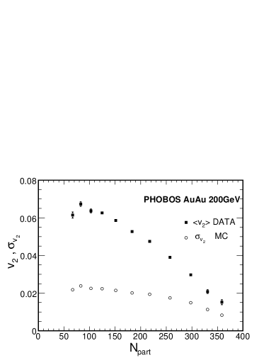
Figure 2: Squares show the average elliptic flow parameter, $v_{2}$, measured near mid-rapidity, as a function of $N_{part}$ for Au+Au collisions at $\sqrt{s_{NN}}=200$ GeV. Only statistical errors are shown. Dots show the RMS of event-by-event $v_{2}$ distribution from PHOBOS Glauber MC (see text.)

Understanding fluctuations in the initial collision region has proven to be crucial to interpret the $\langle v_{2}\rangle$ results. Measurement of $v_{2}$ fluctuations can be used to test the participant eccentricity model. Fig 1 shows a distribution of Glauber model simulated events as a function of $\epsilon_{part}$ and centralityManlyQM . These simulations have been used to caculate the mean, $\langle\epsilon_{part}\rangle$ and the RMS, $\sigma_{\epsilon_{part}}$, of participant eccentricity as a function centrality. Ideal hydrodynamics leads to $v_{2}\propto\epsilon$HydroRef1 . Assuming this holds event-by-event, this condition would imply that:

$$\frac{\sigma_{v_{2}}}{v_{2}}=\frac{\sigma_{\epsilon}}{\epsilon},$$ (3)

where $\sigma_{v_{2}}$ is the RMS of the event-by-event distribution of $v_{2}$. PHOBOS $\langle v_{2}\rangle$ results (Fig. 2) can be used to estimate $\sigma_{v_{2}}$ by Eq. 3. These estimates are also shown in Fig. 2 for Au+Au collisions at $\sqrt{s_{NN}}=200$ GeV. It is important to note that in these estimates, other sources of elliptic flow fluctuations are neglected.

II Method

II.1 Overview

We considered three different methods to measure elliptic flow fluctuations:

• Measuring $\langle v_{2}^{2}\rangle$ via two particle correlations and extracting $v_{2}$ fluctuations by a comparison to the $\langle v_{2}\rangle$ results.

• Measuring $v_{2}^{2}$ event-by-event.

• Measuring $v_{2}$ event-by-event.

Two particle correlations in AA collisions can be used to measure $v_{2}^{2}$Wei . $v_{2}$ fluctuations can be calculated comparing $\langle v_{2}^{2}\rangle$ and $\langle v_{2}\rangle$ by:

$$\sigma_{v_{2}}^{2}=\langle v_{2}^{2}\rangle-\langle v_{2}\rangle^{2}$$ (4)

However, the $\langle v_{2}\rangle$ measurement has significant systematic uncertainties, mainly due to the uncertainties in the reaction-plane determinationPhobosFlowPRC . The $\langle v_{2}^{2}\rangle$ measurement will have systematic uncertainties from various other sources. The comparison of two quantities obtained with different techniques will make it hard to extract precise results. A similar approach has been suggested in Voloshin , where the effects of azimuthal correlations other than flow are also discussed.

Two particle correlations can also be used to make an event-by-event measurement of $v_{2}^{2}$. This method has two main advantages. The first advantage is the possibility to generate a mixed event background to calculate statistical fluctuations. When single hits are mixed, the $v_{2}$ signal disappears whereas when pairs are mixed, the average $v_{2}$ signal is preserved. The second advantage is that there is only one event-by-event fit parameter, $v_{2}^{2}$, since the reaction-plane dependence drops out when the difference between the angles of particles is used. However, non-uniformities in acceptance are very hard to correct for with this approach, since the two-particle acceptance changes event-by-event with respect to the reaction-plane angle.

Conceptually the simplest method is to measure $v_{2}$ event-by-event. In this method, absolute coordinates of the hits in the detector are used to measure $v_{2}$ and the reaction plane. This approach also bears important difficulties. Due to finite number fluctuations, the event-by-event $v_{2}$ resolution is limited. As mentioned above, mixed events generated using single hits have no $v_{2}$ signal and therefore cannot be used as a background reference. Furthermore, the resolution of the measurement changes with the true $v_{2}$ value and the multiplicity in the event.

In this paper, we will concentrate on the last approach. We will describe the method we have developed in order to address the difficulties outlined above for this approach.

In most fluctuation analyses, the statistical fluctuations are calculated using a mixed event background of certain event classes. In this analysis, events in the same event class correspond to events with the same reaction-plane angle. However the reaction-plane angle cannot be measured precisely, making it difficult to generate a mixed event background. Instead, MC simulations of the detector response will be used to account for statistical fluctuations.

In a typical fluctuation measurement of a quantity $x$, the variance of $x$, $\sigma_{x,\text{obs}}^{2}$, can be decomposed into contributions from the statistical fluctuations, $\sigma_{x,\text{stat}}^{2}$, and dynamical fluctuations, $\sigma_{x,\text{dyn}}^{2}$:

$$\sigma_{x,\text{obs}}^{2}=\sigma_{x,\text{dyn}}^{2}+\sigma_{x,\text{stat}}^{2}$$ (5)

This equation holds if the average of the measurement, $\langle x^{obs}\rangle$, gives the true average in the data, $\langle x\rangle$, and if the resolution of the measurement is independent of the true value. Neither of these conditions are satisfied in the event-by-event measurement of $v_{2}$. Therefore, a more detailed study of the response function is required.

We define $K(v_{2}^{obs},v_{2})$ as the distribution of the event-by-event observed elliptic flow, $v_{2}^{obs}$, for events with constant input value of $v_{2}$. If a set of events have an input $v_{2}$ distribution given by $f(v_{2})$, then the distribution of $v_{2}^{obs}$, $g(v_{2}^{obs})$, will be given by:

$$g(v_{2}^{obs})=\int^{\infty}_{0}K(v_{2}^{obs},v_{2})f(v_{2})dv_{2}$$ (6)

It is important to note that Eq. 6 holds in general and Eq. 5 can be derived from it in the special case described above.

Thus, we separate the event-by-event elliptic flow fluctuation analysis into 3 tasks:

• Finding $g(v_{2}^{obs})$ for a set of events, by an event-by-event measurement of $v_{2}^{obs}$.

• Calculating the kernel, $K(v_{2}^{obs},v_{2})$, by studying the detector response.

• Calculating the true $v_{2}$ distribution, $f(v_{2})$, by finding a solution to Eq. 6.

II.2 Event-By-Event Measurement

The PHOBOS detector employs silicon pad detectors to perform tracking, vertex detection and multiplicity measurements. Details of the setup and the layout of the silicon sensors can be found in PhobosDet . The PHOBOS multiplicity array covers a large fraction of the full solid angle. At midrapidity, the vertex detector and the octagonal multiplicity detector have different pad sizes and the acceptance in azimuth is not complete. Fig. 3 shows the distribution of reconstructed hits in the multiplicity array. The event-by-event measurement method has been developed to use all the available information from the multiplicity array to measure a single value, $v_{2}^{obs}$, while allowing an efficient correction for the non-uniformities in the acceptance.

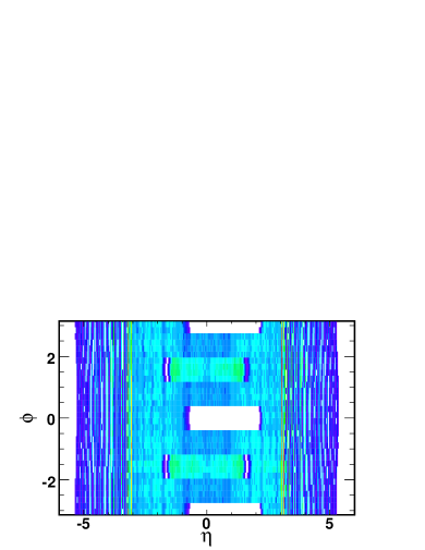
Figure 3: The distribution of reconstructed hits in the PHOBOS multiplicity array for events in a narrow vertex bin.

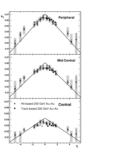
Figure 4: Elliptic flow as a function of pseudorapidity $v_{2}(\eta)$ for charged hadrons for Au+Au collisions at $\sqrt{s_{NN}}=200$ GeV for the three different centrality classes, 25-50%, 15-25% and 3-15% central from top to bottomPhobosFlowPRC . The black lines show the fit given by Eq. 7.

The maximum likelihood method was applied for this purpose. We model the measured pseudorapidity dependence of $v_{2}$ as:

$$v_{2}(\eta)=v_{2}(\eta=0)\cdot(1-|\eta|/6)$$ (7)

This ansatz describes the main feature of the pseudorapidity dependence of $v_{2}$ over a range of centralities, shown in Fig. 4. We will denote $v_{2}(\eta=0)$ shortly as $v_{2}$. We define the probability distribution function (PDF) of a particle to be emitted in the direction $(\eta,\phi)$ for an event with $v_{2}$ and reaction plane angle $\phi_{0}$:

$$P(\eta,\phi|v_{2},\phi_{0})=p(\eta)[1+2v_{2}(\eta)\cos(2(\phi-\phi_{0}))],$$ (8)

where $p(\eta)d\eta$ is the probability for the particle to fall between $\eta$ and $\eta+d\eta$ and $[1+2v_{2}(\eta)\cos(2(\phi-\phi_{0}))]d\phi$ is the probability of the particle to fall between $\phi$ and $\phi+d\phi$. For a single event, the likelihood function of $v_{2}$ and $\phi_{0}$ is defined as:

$$L(v_{2},\phi_{0})=\prod_{i=1}^{n}P(\eta_{i},\phi_{i}|v_{2},\phi_{0}),$$ (9)

where the product is over all $n$ hits in the detector. The likelihood function describes the probability of observing the hits in the event for the given values of the parameters $v_{2}$ and $\phi_{0}$. Treating the hit positions as constants and the parameters $v_{2}$ and $\phi_{0}$ as variables allows choosing an estimate of the parameters, $v_{2}^{obs}$ and $\phi_{0}^{obs}$, which render the likelihood function as large as possible. When comparing different values of $v_{2}$ and $\phi_{0}$ for a given event, $p(\eta)$ is constant and does not contribute to the calculation. However, it is crucial that the PDF folded with the acceptance is normalized to the same value for different sets of parameters $v_{2}$ and $\phi_{0}$. With these considerations, the PDF for hit positions in the detector is redefined. If the acceptance is given by $A(\eta,\phi)$, the normalization constant $s$ is calculated in bins of $\eta$ as:

$$s(v_{2},\phi_{0}|\eta)=\int_{\eta}\,A(\eta^{\prime},\phi)\\ \times[1+2\,v_{2}\,(1-|\eta^{\prime}|/6)\,\cos(2(\phi-\phi_{0}))]\>d\phi\,d\eta^{\prime}$$ (10)

Then the likelihood function becomes:

$$L(v_{2},\phi_{0})=\prod_{i=1}^{n}\,\frac{1}{s(v_{2},\phi_{0}|\eta_{i})}\,\\ \times[1+2\,v_{2}\,(1-|\eta_{i}|/6)\,\cos(2(\phi_{i}-\phi_{0}))]$$ (11)

Instead of maximizing $L(v_{2},\phi_{0})$, it is more convenient for technical reasons to maximize the auxiliary function $l(v_{2},\phi_{0})$, defined as:

$$l(v_{2},\phi_{0})=\sum_{i=1}^{n}\,\ln\Bigl{\{}\frac{1}{s(v_{2},\phi_{0}|\eta_{i})}\,\\ \times\bigl{[}1+2\,v_{2}\,(1-|\eta_{i}|/6)\,\cos\left(2(\phi_{i}-\phi_{0})\right)\bigr{]}\Bigr{\}},$$ (12)

where the sum is over the $n$ reconstructed hits in the detector. Maximizing $l(v_{2},\phi_{0})$ as a function of $v_{2}$ and $\phi_{0}$ allows us to measure $v_{2}^{obs}$ event-by-event.

II.3 The Response Function

To go from the measurement $g(v_{2}^{obs})$ to the true $v_{2}$ distribution, $f(v_{2})$, one needs to determine the response of the measurement. The response function is the kernel in Eq. 6. Finite number fluctuations constitute the major part of the statistical fluctuations. Therefore, the kernel depends on the multiplicity in the detector: $K=K(v_{2}^{obs},v_{2},n)$ where $n$ is the number of reconstructed hits.

Monte Carlo simulations are used to measure $K(v_{2}^{obs},v_{2},n)$. HIJINGHIJING is used to generate Au+Au events. The resulting particles in each event are redistributed in $\phi$ randomly with a probability distribution determined using Eq. 7, according to their $\eta$ positions. These modified events are run through GEANTGEANT to simulate the PHOBOS detector response.

When the event-by-event measurement is done on a set of MC events with a constant value of $v_{2}$ and $n$, it is observed that $K(v_{2}^{obs})|_{v_{2},n}$ is not Gaussian, but is well described by a Gaussian folded by a linear function:

$$K(v_{2}^{obs})|_{v_{2},n}=v_{2}^{obs}\cdot exp\left(-\frac{(v_{2}^{obs}-a)^{2}}{2b^{2}}\right)$$ (13)

as shown in Fig. 5. In the range of the measurement, the parameters $a$ and $b$ have a one-to-one correspondence with $\langle v_{2}^{obs}\rangle$ and $\sigma_{v_{2}^{obs}}$. Therefore, the kernel can be found in MC simulations by measuring the distribution of $v_{2}^{obs}$ in bins of $v_{2}$ and $n$ and calculating $\langle v_{2}^{obs}\rangle$ and $\sigma_{v_{2}^{obs}}$. We use 700,000 events over a collision vertex range of -10 cm$<z<$10 cm in this study, where $z$ is the beam axis direction and the nominal vertex position is $z=0$. The events are divided into 2 cm wide vertex bins. It is worth noting that the vertex resolution, which is better than 400 $\mu$m for a minimum-bias Au+Au eventvertexresolution , is much smaller than the vertex bins used in this analysis. $\langle v_{2}^{obs}\rangle$ and $\sigma_{v_{2}^{obs}}$ are calculated in 70 bins in $v_{2}$ and 8 bins in $n$. The results for one of the vertex bins are shown in Fig. 6. The statistical fluctuations in $v_{2}$ and multiplicity bins limit the precision of our knowledge of the kernel. Fitting smooth functions through the distributions, $\langle v_{2}^{obs}\rangle\,=\,\langle v_{2}^{obs}\rangle\!(v_{2},n)$ and $\sigma_{v_{2}^{obs}}=\sigma_{v_{2}^{obs}}(v_{2},n)$, reduces the bin-by-bin statistical fluctuations and provides a simple parameterization of the kernel. The smooth fits to the results in Fig. 6 are plotted in Fig. 7.

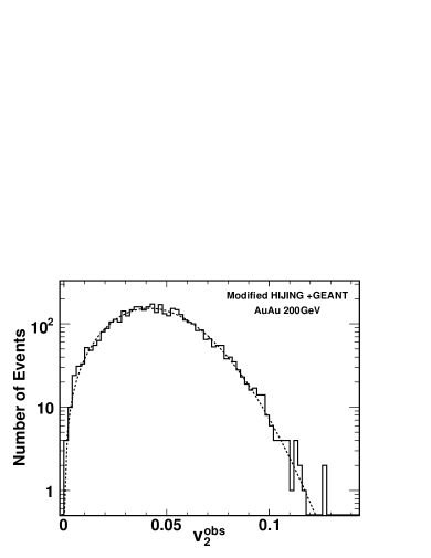
Figure 5: Distribution of the event-by-event measured quantity $v_{2}^{obs}$ for MC events with a constant value of input $v_{2}$ and a small range of hit multiplicity. Dashed line shows fit given by Eq. 13.

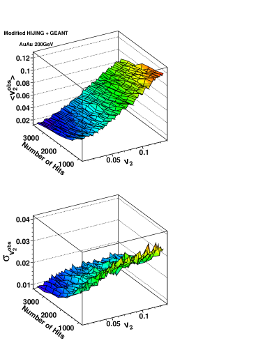
Figure 6: The mean (top) and the RMS (bottom) of the distribution of the event-by-event measured quantity $v_{2}^{obs}$ for MC events in bins of input $v_{2}$ and hit multiplicity.

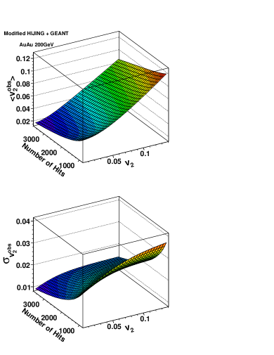
Figure 7: Functions fitted through the distributions shown in Fig. 6.

The analysis is performed in bins of centrality. The paddle detectors which have pseudorapidity coverage of $3.2<|\eta|<4.5$ and cover 2$\pi$ in the azimuthal direction are used in centrality determination. The details of the centrality determination can be found in WhitePaper . Assuming that the true $v_{2}$ distribution, $f(v_{2})$, is independent of the number of hits in the multiplicity array for a set of events in the same centrality class, it is possible to integrate out the multiplicity dependence according to:

$$K(v_{2}^{obs},v_{2})=\int K(v_{2}^{obs},v_{2},n)N(n)dn,$$ (14)

where $N(n)$ is the distribution of number of hits for the set of events. This integration yields the appropriate kernel, plotted in Fig.9, for the given set of events with multiplicity distribution $N(n)$, shown in Fig.8.

II.4 Calculation of Dynamical Fluctuations

As discussed in section II.1, the last step of the analysis is to extract $f(v_{2})$ from $g(v_{2}^{obs})$ and $K(v_{2}^{obs},v_{2})$. There are many possible ways to address this problem. The approach depends on the question that we are trying to answer. In this case, we are interested in the mean and standard deviation of $f(v_{2})$. Therefore we assume an ansatz with two parameters:

$$f(v_{2})=exp\left(-\frac{(v_{2}-\langle v_{2}\rangle)^{2}}{2\sigma_{v_{2}}^{2}}\right)$$ (15)

$f(v_{2})$ is only defined for $v_{2}>0$. Therefore this ansatz is physically meaningful for the values, $\sigma_{v_{2}}/\!\langle v_{2}\rangle\,<<\,1$. The validity of this ansatz, in particular for large $\sigma_{v_{2}}/\!\langle v_{2}\rangle$ will be further studied.

For given values of $\langle v_{2}\rangle$ and $\sigma_{v_{2}}$, it is possible to take the integral in Eq. 6 and calculate the expected distribution $g_{exp}(v_{2}^{obs}|\langle v_{2}\rangle,\sigma_{v_{2}})$. Comparing $g_{exp}(v_{2}^{obs}|\langle v_{2}\rangle,\sigma_{v_{2}})$ with the observation in data and minimizing the $\chi^{2}$ defined as:

$$\chi^{2}=\sum_{v_{2}^{obs}bins}\frac{[g(v_{2}^{obs})\,-\,g_{exp}(v_{2}^{obs}|\langle v_{2}\rangle,\sigma_{v_{2}})]^{2}}{g(v_{2}^{obs})}$$ (16)

values of $\langle v_{2}\rangle$ and $\sigma_{v_{2}}$ can be obtained.

II.5 Verification of the Complete Analysis Chain

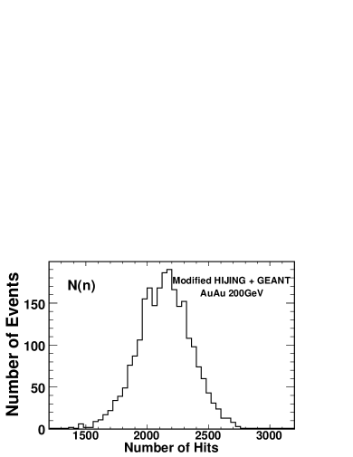
Figure 8: Distribution of the observed number of hits for a set of events.

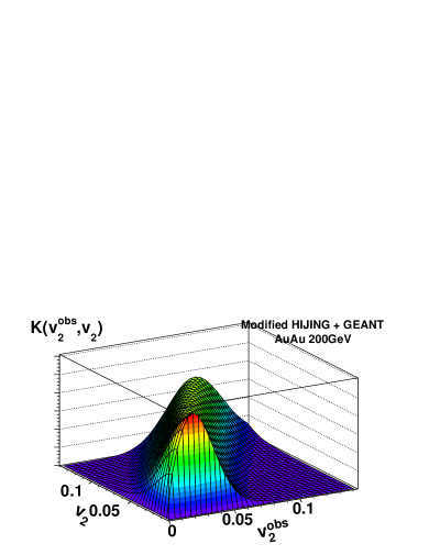
Figure 9: The kernel calculated for the set of events with multiplicity distribution shown in Fig. 8 according to Eq. 14.

Figure 10: The true $v_{2}$ distribution for a set of selected MC events with multiplicity distrubution shown in Fig. 8. Smooth line shows the parent Gaussian distribution.

Figure 11: Distribution of the event-by-event measured quantity, $v_{2}^{obs}$, for the set of events with the multiplicity distribution in Fig. 8 and input $v_{2}$ distribution in Fig. 10.

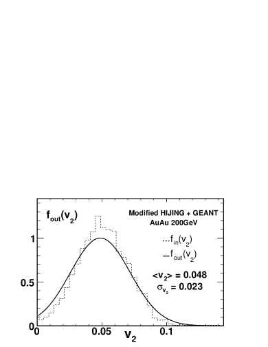
Figure 12: Solid line shows the reconstructed $v_{2}$ distribution for the set of events with input $v_{2}$ distribution shown in dashed lines (also in Fig. 10) and kernel shown in Fig. 9.

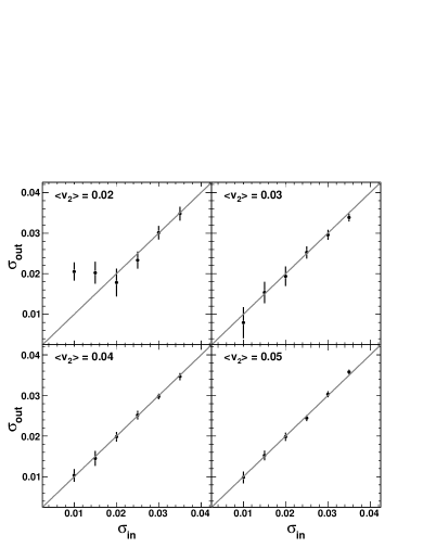
Figure 13: Reconstructed $\sigma_{v_{2}}$ as a function of input $\sigma_{v_{2}}$ for different sets of 15-20% central MC events. Plots are shown for input $\langle v_{2}\rangle\>=0.02$ (top left), 0.03 (top right), 0.04 (bottom left) and 0.05 (bottom right). Statistical errors from combining 10 different vertex bins are shown.

The whole analysis procedure was tested using sets of MC events, selected from the events used to construct the kernel. Approximately 20,000 15-20% central events with a Gaussian distribution of $v_{2}$ were used to construct each set. It should be noted that the functional form of the distribution of $v_{2}$ in these sets is the same as our ansatz(Eq. 15) and the pseudorapidity dependence of $v_{2}$ is the same as in our PDF(Eq. 7). Sample sets were selected with $\langle v_{2}\rangle=0.02,$ 0.03, 0.04 and 0.05. For each value of $\langle v_{2}\rangle$, six different values of $\sigma_{v_{2}}$ (0.01, 0.015, 0.02, 0.025, 0.03, 0.035) were chosen. Each set was divided in the 10 collision vertex bins, for which the kernels were constructed. The multiplicity distribution $N(n)$, the kernel $K(v_{2}^{obs},v_{2})$, the input distribution $f_{in}(v_{2})$ and the measured distribution $g(v_{2}^{obs})$ are plotted in Figures 8, 9, 10, and 11 for a set of events from one vertex bin with $\langle v_{2}\rangle=0.05$ and $\sigma_{v_{2}}=0.02$. Minimizing the $\chi^{2}$ defined in Eq. 16, yields the estimate of the true $\langle v_{2}\rangle$ and $\sigma_{v_{2}}$ from the measurement. For this set, the values were found to be $\langle v_{2}\rangle=0.048$ and $\sigma_{v_{2}}=0.023$. The Gaussian distribution with these values is the estimate of the true $v_{2}$ distribution from the measurement. The distribution is plotted in Fig. 12 together with the true MC $v_{2}$ ditribution.

Results obtained from different vertex bins were averaged. Fig. 13 shows the combined results. It is seen that the method successfully reconstructs the input fluctuations down to $\langle v_{2}\rangle\approx 0.03$.

III Conclusion and Outlook

The participant eccentricity model has increased the interest in measuring elliptic flow fluctuations. We have introduced a new analysis approach to perform this measurement. In this approach, all the available information from the PHOBOS multiplicity array is used to determine $v_{2}$ event-by-event. The response function of the event-by-event measurement, containing the contribution of statistical fluctuations and detector effects is calculated using Monte Carlo simulations. Non-statistical fluctuations are extracted by unfolding the response function from the distribution of the event-by-event measurement. Our approach has been tested on small sets of MC events, selected from the events used to calculate the response function. The input fluctuations are reconstructed successfully for $\langle v_{2}\rangle\geq 0.03$.

The analysis can readily be applied to real data. The next step in the analysis will be to systematically study how the differences between HIJING MC and data in $dN/d\eta$, $v_{2}(\eta)$ and azimuthal correlations other than flow influence the results. Different MC event generators and MC events with different input $v_{2}(\eta)$ distributions will be used for this purpose.

This work was partially supported by U.S. DOE grants DE-AC02-98CH10886, DE-FG02-93ER40802, DE-FC02-94ER40818, DE-FG02-94ER40865, DE-FG02-99ER41099, and W-31-109-ENG-38, by U.S. NSF grants 9603486, 0072204, and 0245011, by Polish KBN grant 1-P03B-062-27(2004-2007), by NSC of Taiwan Contract NSC 89-2112-M-008-024, and by Hungarian OTKA grant (F 049823).

References

- (1) J.-Y. Ollitrault, Phys. Rev. D46, 229 (1992)
- (2) E877 Collaboration, J. Barrette et al., Phys. Rev. C55, 1420 (1997)
- (3) E895 Collaboration, C. Pinkenburg et al., Phys. Rev. Lett. 83, 1295 (1999)
- (4) NA49 Collaboration, H. Appelshäuser et al., Phys. Rev. Lett. 80, 4136 (1998)
- (5) WA98 Collaboration, M.M. Aggarwal et al., Phys. Lett. B403, 390 (1997); M.M. Aggarwal et al., Nucl. Phys. A638, 459 (1998)
- (6) K.H. Ackermann et al. [STAR Collaboration], Phys. Rev. Lett. 86, 402 (2001)
- (7) B. B. Back et al. [PHOBOS Collaboration], Phys. Rev. Lett. 89, 222301 (2002)
- (8) B. B. Back et al. [PHOBOS Collaboration], Phys. Rev. Lett. 95, 122303 (2005)
- (9) B.B. Back et al. [PHOBOS Collaboration], Phys. Rev. C72, 051901(R) (2005)
- (10) S. Manly et al. [PHOBOS Collaboration], arXiv:nucl-ex/0510031
- (11) P. F. Kolb, P. Huovinen, U. W. Heinz, H. Heiselberg, Phys. Lett. B500, 232 (2001)
- (12) B. B. Back et al. [PHOBOS Collaboration], Nucl. Phys. A757, 28 (2005)
- (13) S. Mrowczynski, E. Shuryak, Acta Phys.Polon. B34, 4241 (2003)
- (14) M. Miller, R. Snellings, arXiv:nucl-ex/0312008
- (15) W. Li et al. [PHOBOS Collaboration], These proceedings
- (16) S. A. Voloshin, arXiv:nucl-th/0606022
- (17) B.B. Back et al., Nucl. Instrum. Meth. A 499, 603 (2003)
- (18) M. Gyulassy and X. N. Wang, Comput. Phys. Commun. B 83, 307 (1994)
- (19) R. Brun et al., GEANT3 Users Guide, CERN DD/EE/84-1
- (20) B.B. Back et al., Phys. Rev. Lett. 88, 22302 (2002)