Inclusive Electron Scattering From Nuclei
at $x>1$ and High $Q^{2}$

Abstract

CEBAF experiment e89-008 measured inclusive electron scattering from nuclei in a $Q^{2}$ range between 0.8 and 7.3 (GeV/c)² for $x_{Bjorken}\mathrel{\raise 1.29167pt\hbox{$>$}\mkern-14.0mu\lower 2.58334pt\hbox{$\sim$}}1$. The cross sections for scattering from D, C, Fe, and Au were measured. The C, Fe, and Au data have been analyzed in terms of F($y$) to examine $y$-scaling of the quasielastic scattering, and to study the momentum distribution of the nucleons in the nucleus. The data have also been analyzed in terms of the structure function $\nu W_{2}$ to examine scaling of the inelastic scattering in $x$ and $\xi$, and to study the momentum distribution of the quarks. In the regions where quasielastic scattering dominates the cross section (low $Q^{2}$ or large negative values of $y$), the data are shown to exhibit $y$-scaling. However, the $y$-scaling breaks down once the inelastic contributions become large. The data do not exhibit $x$-scaling, except at the lowest values of $x$, while the structure function does appear to scale in the Nachtmann variable, $\xi$.

Chapter 1 Introduction

1.1 Experiment Overview

Electron scattering provides a powerful tool for studying the structure of the nucleus. Because the electron-photon interaction is well described by QED, electron scattering provides a well understood probe of nuclear structure. The electromagnetic interaction between the electron and the target is very weak, which allows the electron to probe the entire target nucleus. In inclusive electron scattering, where only the scattered electron is detected, the final-state interactions (FSI) between the electron and the nucleus are expected to be small and decrease rapidly with momentum transfer [1, 2, 3, 4, 5, 6, 7, 8]. The well understood reaction mechanism and small FSI corrections allow a clean separation of the scattering mechanism from the structure of the target.

Because the electromagnetic interaction is relatively weak, it is well modeled by the exchange of a single virtual photon between the incident electron and a single particle in the nucleus. The ‘particle’ probed by the interaction can vary depending on the kinematics of the scattering. At extremely low energy transfers, the photon interacts with the entire nucleus, scattering elastically or exciting a nuclear state or resonance. At somewhat higher energy and momentum transfers, scattering is dominated by quasielastic (QE) scattering, where the photon interacts with a single nucleon. As the energy and momentum transfer increase, and the photon probes smaller distance scales, the interaction will become sensitive to the quark degrees of freedom in the nucleus. For sufficiently hard interactions, the mechanism is primarily scattering from a single quark. As the momentum transfer increases, the time scale of the photon-quark interaction decreases, and it is expected that at high enough momentum transfers, the electron will be nearly unaffected by the subsequent interactions of the struck quark, and the scattering is well approximated by elastic scattering from a free (but moving) quark.

In addition to the clean separation of the scattering process from the structure of the target, electron scattering from a nucleus is well suited to examination of the structure of the nucleus. Because electron scattering from a free nucleon is a well-studied problem, one can try to separate the structure of the nucleon from the structure of the nucleus, and examine the nuclear structure, as well as modifications to the structure of the nucleons in the nuclear medium. The structure of the nucleus was shown to be non-trivial with the discovery of the EMC effect [9]. Electron scattering can provide additional information on nuclear modifications to the nucleon structure, and can extend the measurement of the EMC effect into a new kinematic regime.

CEBAF experiment e89-008 was designed to study the structure of the nucleus by measuring inclusive scattering from nuclei over a wide kinematic range. The kinematics were chosen to make the energy transfer as small as possible, while increasing the 4-momentum transfer, $Q^{2}$, as high as possible. By choosing small energy transfers, we select the quasielastic scattering from a single nucleon, even as we increase $Q^{2}$. In this way, we can study the quasielastic scattering at values of $Q^{2}$ where inelastic scattering usually dominates, even on top of the quasielastic peak. In order to measure at these high values of 4-momentum transfer, a high energy electron beam (several GeV) is required. The cross sections at low energy loss are small, and fall rapidly with increasing momentum transfer. Therefore, it was necessary to have a very high current beam in order to measure the cross section. CEBAF provides a CW electron beam with energies of up to 4 GeV and currents up to 100 $\mu$A, providing both the energy and luminosity necessary for this experiment.

The experiment measured the cross section over a wide range of energy transfers, allowing us to study how the scattering mechanism changes as we move from probing the individual nucleons to probing the quarks. In order to study the individual scattering processes, the data were analyzed in terms of scaling functions which are expected to show a specific behavior for either quasielastic scattering or deep inelastic scattering. Data were taken for a variety of target nuclei (D,C,Fe,Au) in order to examine the effects of the nuclear medium for different nuclei.

In this experiment, we know the initial electron energy and momentum ($E,\vec{k}$), and measure the electron’s energy and momentum after scattering ($E^{\prime},\vec{k}^{\prime}$). This fully determines the kinematics at the electron vertex, and gives us the energy ($E-E^{\prime}$) and momentum ($\vec{k}-\vec{k}^{\prime}$) of the virtual photon. The scattering kinematics are usually described in terms of two variables: the energy transfer, $\nu=E-E^{\prime}$, and the square of the 4-momentum transfer, $Q^{2}=-q_{\mu}q^{\mu}=|\vec{k}-\vec{k}^{\prime}|^{2}-(E-E^{\prime})^{2}$. In addition, one can define the Bjorken $x$ variable, $x={Q^{2}\over 2m\nu}$, where m is the mass of the nucleon. For scattering from a free nucleon, $x$ can vary between 0 and 1, where $x=1$ corresponds to elastic scattering from the nucleon, and $x<1$ corresponds to inelastic scattering. In the limit of large $\nu$ and $Q^{2}$, it can be shown in the parton model that $x$ is the fraction of the nucleon’s momentum (parallel to $\vec{q}$) that was carried by the struck quark [10] and the dimensionless structure function $\nu W_{2}(x)$ represents the charge-weighted momentum distribution of the quarks making up the nucleon. In a nucleus, the nucleons share momentum, so that $x$ can vary between 0 and $A$, the total number of nucleons. Therefore, measuring scattering at $x>1$ probes the effect of the nuclear medium on the quark distributions within individual nucleons.

Selecting appropriate scattering kinematics allows us to examine the different scattering processes. For elastic scattering from the nucleus, the electron is interacting with the entire nucleus, and so the scattering occurs at $x=A$. If the nucleus is knocked into an excited state, there is some additional energy loss, and $x$ will decrease from $A$ as the energy loss increases. At somewhat higher energy loss, where quasielastic scattering is the dominant process, the electron knocks a single nucleon out of the nucleus. This corresponds to scattering near $x=1$, where the struck object contains (on average) $1/A$ of the total momentum of the $A$ nucleons. At higher energy transfers, corresponding to $x<1$, the scattering is inelastic and the struck nucleon is either excited into a higher energy state (in resonance scattering), or broken up completely (in deep inelastic scattering). At very high energy transfers, where deeply inelastic scattering dominates, the electron is primarily interacting with a single quark.

1.2 Scaling Functions

In inclusive electron scattering, scaling functions are a useful way to examine the underlying structure of a complex system. Scaling behavior of a system tends to indicate a simple underlying mechanism or substructure in the system. In the case of electron scattering, where the interaction mechanism is simple and well understood, examining the data in terms of scaling functions allows one to study the substructure of the nucleus. For unpolarized inclusive electron scattering, the cross section can be written in the following general form:

$${{d\sigma}\over{dE^{\prime}d\Omega}}={{4\alpha^{2}E^{\prime 2}}\over{Q^{4}}}\ \biggl{[}W_{2}(\nu,Q^{2})\cos^{2}(\theta/2)+2W_{1}(\nu,Q^{2})\sin^{2}(\theta/2)\biggr{]},$$ (1.1)

where $W_{1}(\nu,Q^{2})$,$W_{2}(\nu,Q^{2})$ are two independent inelastic structure functions describing the structure of the nucleus. For very low energy scattering, the electron scatters from the nucleus as a whole, and the sub-structure of the nucleus is not ‘visible’ to the electron probe. In this case, the structure functions are simplified to the product of a $\delta$-function, $\delta(\nu+{Q^{2}\over 2M_{A}}$), and a function which now depends only on $Q^{2}$, rather than $\nu$ and $Q^{2}$. This is a case of scaling, where the general form of the scattering (Eqn. 1.1) is simplified because of the simplified reaction mechanism in the limit of low energy transfer. If you were to measure the scattering cross section and find that it reduced to this form, it would be a strong indication that the scattering is well described by scattering from a structureless nucleus, even though there may be an underlying structure to which you are not sensitive.

In addition to looking for a simple structure of the target, one can examine the behavior of the scaling function itself. The scaling function contains information about the structure of the system, and violations of expected scaling behavior can be studied in order to understand the validity of assumptions in the model that predicts scaling. We will be examining scaling functions for two simplified cases of the general scattering. First we will examine quasielastic (QE) scattering, where the electron interacts with a single nucleon in the nucleus. We will also examine deep inelastic scattering (DIS), where the electron interacts with a single, quasi-free quark.

1.3 Quasielastic Scattering: $y$-scaling

If one assumes that the quasielastic scattering is well described by the exchange of a photon with a single nucleon, it can be shown that the cross section will show a scaling behavior [11, 12, 13]. In the plane-wave impulse approximation (PWIA), the exclusive cross section for quasielastic A(e,e’N) scattering can be written as the sum over cross sections for the individual (bound) nucleons:

$${{d^{5}\sigma}\over{dE^{\prime}d\Omega d^{3}\vec{p}^{\prime}}}=\sum_{nucleons}\sigma_{eN}\cdot S^{\prime}_{N}(E_{0},\vec{p}_{0}),$$ (1.2)

where $E^{\prime}$ is the energy of the scattered electron, $E_{0}$ and $\vec{p}_{0}$ are the initial energy and momentum of the struck nucleon, and $\vec{p}^{\prime}$ is the final momentum of the struck nucleon. $S^{\prime}_{N}(E_{0},\vec{p}_{0})$ is the spectral function (the probability of finding a nucleon with energy $E_{0}$ and momentum $\vec{p}_{0}$ in the nucleus) and $\sigma_{eN}$ is the electron-nucleon cross section for scattering from a bound (off-shell) nucleon.

The inclusive cross section will be an integral over the nucleon final states of the exclusive cross section, and therefore an integral over the spectral function. However, if we consider only quasielastic scattering and neglect final-state interactions, the cross section for inclusive quasielastic scattering can (with appropriate assumptions), be reduced to the following form (see sections 4.2 and 4.3):

$${d\sigma\over{d\Omega dE^{\prime}}}=\sigma_{eN}\cdot F(y),$$ (1.3)

where $y$ corresponds to the nucleon’s momentum along the direction of the virtual photon, and $F(y)$ is the scaling function, which is closely related to the momentum and energy distribution of the nucleons. Now, rather than a convolution of the cross section with the structure function, the cross section separates into two terms. The first term ($\sigma_{eN}$) represents the interaction process while the other term ($F(y)$) represents the nuclear structure. $F(y)$ represents the momentum distribution of the struck nucleon (parallel to $\vec{q}$), and is closely related to the spectral function (section 4.3).

If we measure the cross section over a range of $y$ and $Q^{2}$ values, and divide out the elementary e-N cross section, the model predicts that the result should be independent of $Q^{2}$. If it is, then we have a good indication that we are seeing quasielastic scattering, even though we do not directly measure anything about the hadron final state. Observing scaling also provides evidence that the PWIA model of the scattering is correct and sufficient to describe the scattering. In addition, by measuring the scaling function, we are probing the momentum distribution of the nucleons in the nucleus. Even if the scaling is not perfect, we can use the observed $Q^{2}$ dependence to learn something about the system. At low $Q^{2}$, final-state interactions are large, contradicting the assumptions of the PWIA model and causing the scaling behavior to break down. The approach to scaling at low $Q^{2}$ will be sensitive to the details of the final-state interactions, and we can look at the breakdown of scaling in order to try and understand the final-state interactions. At high $Q^{2}$, the scattering will become inelastic, and the PWIA will break down, leading to a failure of the scaling. Examining the scaling function in this region is one way to examine the transition from quasielastic scattering to deep inelastic scattering.

1.4 Deep Inelastic Scattering: $x$-scaling

As we increase $\nu$ and $Q^{2}$, the virtual photon probes shorter distances and becomes sensitive to the quark structure of the nucleon. As the energy and momentum transfer increase, the interaction occurs over a shorter time period and over smaller distance scales. Thus, the electron should become less sensitive to the interactions of the struck quark with the other partons. If we assume that in the limit of large $\nu$ and $Q^{2}$, the electron only sees a single, quasi-free quark, then we can write down the general form for unpolarized inclusive electron-nucleon scattering,

$${{d\sigma}\over{dE^{\prime}d\Omega}}={{4\alpha^{2}E^{\prime 2}}\over{Q^{4}}}\ \biggl{[}W_{2}(\nu,Q^{2})\cos^{2}(\theta/2)+2W_{1}(\nu,Q^{2})\sin^{2}(\theta/2)\biggr{]}$$ (1.4)

and compare it to elastic scattering from a stationary, point-like, spin-$\frac{1}{2}$ object,

$${{d\sigma}\over{dE^{\prime}d\Omega}}={{4\alpha^{2}E^{\prime 2}}\over{Q^{4}}}\ \biggl{[}\cos^{2}(\theta/2)+{Q^{2}\over 2m^{2}}\sin^{2}(\theta/2)\biggr{]}\delta(\nu-{Q^{2}\over 2m}).$$ (1.5)

Equating these expressions for the cross sections gives us the following form for the structure functions:

$$W_{1}={Q^{2}\over 4m^{2}}\delta(\nu-{Q^{2}\over 2m})$$ (1.6)

$$W_{2}=\delta(\nu-{Q^{2}\over 2m}).$$ (1.7)

Rearranging the arguments of the $\delta$ function, and choosing dimensionless versions of the structure functions gives the following:

$$2mW_{1}={Q^{2}\over 2m\nu}\delta(1-{Q^{2}\over 2m\nu})$$ (1.8)

$$\nu W_{2}=\delta(1-{Q^{2}\over 2m\nu}).$$ (1.9)

So if we assume that in the limit of large $\nu$ and $Q^{2}$ the electron-quark interaction is independent of the other partons and the electron is unaffected by final-state interactions of the struck quark, then the structure functions take on simplified forms. In this case, the structure functions become functions of Bjorken $x={Q^{2}\over 2m\nu}$ rather than functions of $\nu$ and $Q^{2}$ independently. In the limit of $\nu,Q^{2}\rightarrow\infty$, $x$ is interpreted as the fraction of the nucleon’s momentum carried by the struck quark ($0<x<1$) and the structure function in the scaling limit then represents the momentum distribution of the quarks (see section 4.4 or [14]).

In low-$x$ scattering from protons, the structure functions have been measured to extremely high $Q^{2}$ and show scaling in $x$. The observation of the expected scaling is a strong indication that the parton model of the proton is correct, and that there is a quark substructure to the proton. The measured structure functions in the scaling limit give information about the momentum distribution of the quarks. In addition, the low $Q^{2}$ behavior, which does not show scaling, is interesting when looking for low-$Q^{2}$ scaling violations and so called higher-twist effects [15] arising from quark final-state interactions. These higher-twist scaling violations decrease with increasing momentum transfer at least as fast as $1/Q^{2}$. Deviations from perfect $x$-scaling are also expected (and observed) at high $Q^{2}$ due to the running QCD coupling constant, $\alpha_{s}(Q^{2})$. As was the case with $y$-scaling, both the observation of scaling in $x$ and measurements of the deviations from scaling are of interest. Figure 1.1 shows the proton structure function, $F_{2}^{p}$ as a function of $Q^{2}$ for several $x$ bins. For all values of $x$, the $Q^{2}$ dependence of $F_{2}(x,Q^{2})$ becomes small as $Q^{2}$ increases. However, even at the largest $Q^{2}$ values, there are still scaling violations. The QCD scaling violations lead to an increase in strength at low $x$, and a decrease at high $x$ as $Q^{2}$ increases. As the wavelength of the photon decreases, it becomes sensitive to a wider range of parton $x$ values. The high-$x$ partons are resolved as a quark at somewhat lower $x$ surrounded by lower momentum partons (quarks and gluons), and so fewer partons are observed at large $x$, and more are observed at very low $x$.

Figure 1.1: Proton structure function, $F_{2}^{p}$, from lepton-proton scattering data. A constant has been added to $F_{2}^{p}$ for each $x$ bin. Errors shown are statistical. (Figure from the Particle Data Group [16].)

In electron-Nucleus scattering, exactly as with electron-Nucleon scattering, one can equate the structure functions for the nucleus with the elastic electron-parton cross section and find that the structure function for the nucleus should depend only on $x$ as $Q^{2}\rightarrow\infty$. Scaling of the inelastic nuclear structure function should occur at large $Q^{2}$, but now the momentum distribution of the quarks is modified by the nucleon-nucleon interactions in the nucleus, and $x$ can vary between 0 and $A$, rather than 0 and 1. Figure 1.2 shows $F_{2}^{d}$ as a function of $Q^{2}$ for several $x$ bins. Note that the scaling behavior is essentially identical for the proton and deuteron structure functions, but that the value of $F_{2}^{d}$ as a function of $x$ differs from $F_{2}^{p}$. The structure function for the proton is larger than for the deuteron at low values of $x$ and nearly identical for the larger values of $x$ shown. For $x>1$, the proton structure function is zero, while the deuteron structure function can be non-zero up to $x=2$.

Figure 1.2: Deuteron structure function, $F_{2}^{d}$, from lepton-deuteron scattering data. A constant has been added to $F_{2}^{d}$ for each $x$ bin. Errors shown are statistical. (Figure from the Particle Data Group [16].)

1.5 $\xi$-scaling and Local Duality

The scaling of the deep inelastic structure function at large $Q^{2}$ has been observed in inclusive scattering from a free nucleon. At low $Q^{2}$, violations of $x$-scaling are caused by resonance scattering and other higher-twist effects. At higher $Q^{2}$, the logarithmic $Q^{2}$ dependence of the strong coupling constant leads to scaling violations. In order to study the QCD scaling violations at finite $Q^{2}$, it is necessary to disentangle them from the low-$Q^{2}$ scaling violations caused by higher-twist effects. Georgi and Politzer [17] showed that in order to study the scaling violations at finite $Q^{2}$, the Nachtmann variable $\xi=2x/[1+(1+4M^{2}x^{2}/Q^{2})^{1/2}]$ was the correct variable to use. As $Q^{2}\rightarrow\infty$, $\xi\rightarrow x$, and so the scaling expected in $x$ should also be observed in $\xi$ in the limit of large $\nu$ and $Q^{2}$. However, using $\xi$ rather than $x$ at finite $Q^{2}$ accounts for the finite target mass effects which otherwise mask the QCD scaling violations.

In addition to the $\log(Q^{2})$ QCD scaling violations, higher-twist (O($m^{2}/Q^{2}$)) contributions from resonances are large at finite $Q^{2}$. It has been shown [18, 19] that as $x\rightarrow 1$ the nucleon structure functions connect smoothly with the elastic form factors. In addition, it was observed by Bloom and Gilman [20] that the resonance form factors and nucleon inelastic structure functions have the same $Q^{2}$ dependence when examined as a function of $\omega^{\prime}=1/x+M^{2}/Q^{2}=1+W^{2}/Q^{2}$. Figure 1.3 shows the structure function in the resonance region as a function of $\omega^{\prime}$ for several values of $Q^{2}$ [21], along with the high-$Q^{2}$ limit of the inelastic structure function [22]. While the resonance form factors clearly have a large $Q^{2}$ dependence, if the resonances are averaged over a finite region of $\omega^{\prime}$, they reproduce the scaling limit of the inelastic structure functions. It was later shown [23] that this ‘local duality’ of the resonance form factors and inelastic structure functions was expected from perturbative QCD, and that this duality should extend to the nucleon elastic form factor if the structure function is examined in terms of $\xi$.

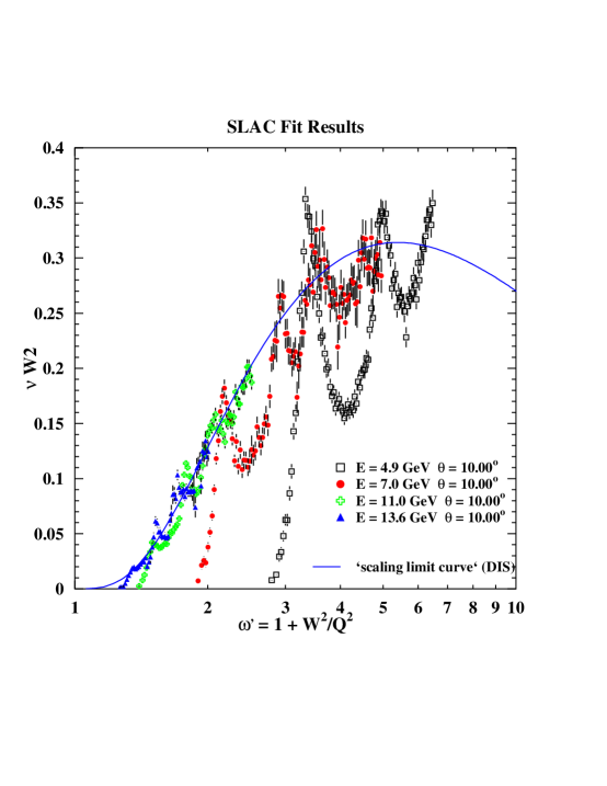
Figure 1.3: Proton resonance structure function versus the deep inelastic limit. The data are from SLAC experiment E133 [21]. The scaling limit curve is from [22].

1.6 Previous Data

A significant amount of inclusive electron scattering data exists for $x\mathrel{\raise 1.29167pt\hbox{$>$}\mkern-14.0mu\lower 2.58334pt\hbox{$\sim$}}1$, up to extremely high $Q^{2}$. However, nearly all of the data is taken on top of the quasielastic peak, near $x=1$. At the top of the QE peak, contributions from inelastic scattering become large at $Q^{2}\sim 2$ (GeV/c)² [24, 25]. In order to measure quasielastic scattering at higher momentum transfer without having to subtract out the inelastic contribution, one needs to go to smaller values of energy loss (corresponding to $y<0$ or $x>1$). There is not a significant amount of data taken for energy losses below the elastic peak on nuclear targets. For deuterium, there is data for $x\leq 2$ up to $Q^{2}\approx$4 (GeV/c)², and data at $x\mathrel{\raise 1.29167pt\hbox{$<$}\mkern-14.0mu\lower 2.58334pt\hbox{$\sim$}}1.2$ up to $Q^{2}\approx 10$ (GeV/c)² [26, 27, 28]. There is also a significant amount of data taken for ³He [29, 30, 27], for momentum transfers up to 2.2 GeV/c. There is significantly less data available on heavier nuclei. For $x$ somewhat larger than 1, there are results on Carbon from BCDMS [31] and in Iron from CDHSW [32] for similar $Q^{2}$ ranges ($50\mathrel{\raise 1.29167pt\hbox{$<$}\mkern-14.0mu\lower 2.58334pt\hbox{$\sim$}}Q^{2}\mathrel{\raise 1.29167pt\hbox{$<$}\mkern-14.0mu\lower 2.58334pt\hbox{$\sim$}}200$ (GeV/c)²), and results on Iron from NuTeV at Fermilab [33] for $Q^{2}>50(GeV/c)^{2}$. However, the BCDMS and CDHSW data only provide upper limits for $x>1.1$ and the Fermilab data only goes up to $x\approx 1.15$. The only data with coverage significantly above $x=1$ comes from the SLAC end-station A experiment NE3 [34, 24, 35]. This experiment measured inclusive electron scattering on ⁴He, C, Al, Fe, and Au for 0.23$<Q^{2}<$3.69 (GeV/c)², and $x\mathrel{\raise 1.29167pt\hbox{$<$}\mkern-14.0mu\lower 2.58334pt\hbox{$\sim$}}3$. In addition, there is Aluminum data for $1<x<2$, which was taken as dummy target data for Deuterium measurements [36].

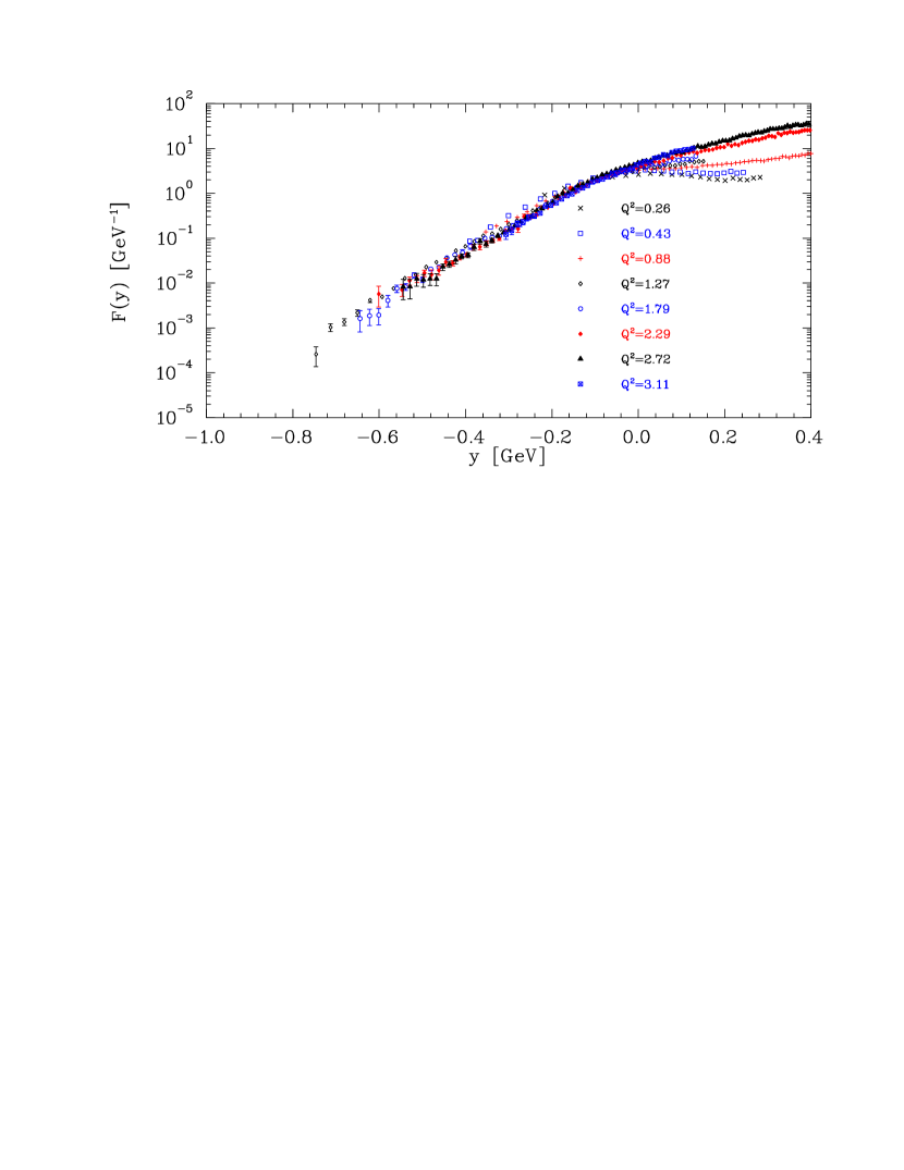
Figure 1.4: $F(y)$ for Iron from SLAC experiment NE3. The different curves represent different values of beam energy and spectrometer angle and are labeled by the value of $Q^{2}$ at $x=1$. Errors shown are statistical only. $F(y)$ has been recalculated from the NE3 cross sections using a new value for $E_{s}^{0}$ (see section 5.2).

Figure 1.4 shows the NE3 data for Iron, analyzed in terms of the scaling function $F(y)$. For all targets, the data show scaling in $y$ at large $Q^{2}$ and negative values of $y$. Significant scaling violations were observed at low $Q^{2}$ due to final-state interactions, and at $y\mathrel{\raise 1.29167pt\hbox{$>$}\mkern-14.0mu\lower 2.58334pt\hbox{$\sim$}}0$, where inelastic contributions to the cross section begin to become significant. The scaling violations at low $Q^{2}$ increase for high-$A$ nuclei and at large $|y|$, where the final-state interactions are largest. Figure 1.5 shows the $Q^{2}$ dependence of $F(y)$ for fixed values of $y$ on the low energy loss side of the quasielastic peak. As $Q^{2}$ increases, these scaling violations decrease, and for $Q^{2}\mathrel{\raise 1.29167pt\hbox{$>$}\mkern-14.0mu\lower 2.58334pt\hbox{$\sim$}}2.5$ [GeV/c]², the data appear to be to approaching a scaling limit. However, the uncertainties in these high-$Q^{2}$ points are relatively large, and there are very few points above $Q^{2}=2.5$. Because of this, it is difficult to determine if the scaling limit has been reached and if the final-state interactions truly are small in this region of momentum transfer. For $y\mathrel{\raise 1.29167pt\hbox{$>$}\mkern-14.0mu\lower 2.58334pt\hbox{$\sim$}}0$, inelastic contributions are large, and grow as $Q^{2}$ and $y$ increase. In this region, the PWIA approximation is not valid and the prediction of $y$-scaling is not applicable.

Figure 1.5: $F(y)$ versus $Q^{2}$ for Iron from NE3. $F(y)$ is shown for four values of $y$, with a scaling factor applied for each $Q^{2}$. Errors shown are statistical only. There is a systematic uncertainty of 3.5-3.7%.

Figure 1.6 shows the measured structure function for Iron. At low $x$ values ($x\mathrel{\raise 1.29167pt\hbox{$<$}\mkern-14.0mu\lower 2.58334pt\hbox{$\sim$}}0.5$), the scattering is inelastic, and the structure function shows scaling for sufficiently large values of $Q^{2}$. For $x\mathrel{\raise 1.29167pt\hbox{$>$}\mkern-14.0mu\lower 2.58334pt\hbox{$\sim$}}1$, the data do not show scaling in $x$. Scaling in $x$ is expected in the region where the interaction is well described by quasi-free electron-quark scattering. In the quasielastic region, the electron interacts with the entire nucleon, and one does not expect to see scaling in x. The fact that the data show scaling in $y$ for negative $y$ indicates that the scattering is dominated by quasielastic scattering. Therefore, for $x\mathrel{\raise 1.29167pt\hbox{$>$}\mkern-14.0mu\lower 2.58334pt\hbox{$\sim$}}1$ (which approximately corresponds to $y\mathrel{\raise 1.29167pt\hbox{$<$}\mkern-14.0mu\lower 2.58334pt\hbox{$\sim$}}0$) we do not expect to observe $x$-scaling.

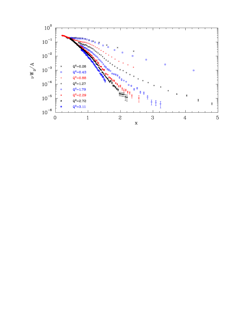
Figure 1.6: Structure Function $\nu W_{2}$ vs. $x$ for Iron from SLAC experiment NE3. The different curves represent different values of beam energy and spectrometer angle and are labeled by the value of $Q^{2}$ at $x=1$. Errors shown are statistical only.

If $\xi$ is simply a modified version of $x$, designed to improve scaling at lower $Q^{2}$, then the structure function should show improved scaling at low $\xi$, where the $x$-scaling appears to be valid. It should not show scaling at large $\xi$, where the scattering is primarily quasielastic. However, when the structure function is plotted versus $\xi$ (figure 1.7), a different behavior is observed. The data appear to approach a universal curve at all values of $\xi$ as $Q^{2}$ increases. The success of $\xi$-scaling in the quasielastic region may come from the local duality observed in inclusive scattering from free protons. In the case of scattering from a proton, the resonance form factors have the same $Q^{2}$ dependence as the inelastic structure function when averaged over a range in $\xi$. When scattering from a nucleus, the momentum distribution of the nucleons can provide an averaging of the structure function. If this averaging is over a large enough region to smooth the individual quasi-elastic and resonance peaks, then the quasielastic and resonance scattering should match the inelastic structure function, as appears to happen for the data at larger $Q^{2}$.

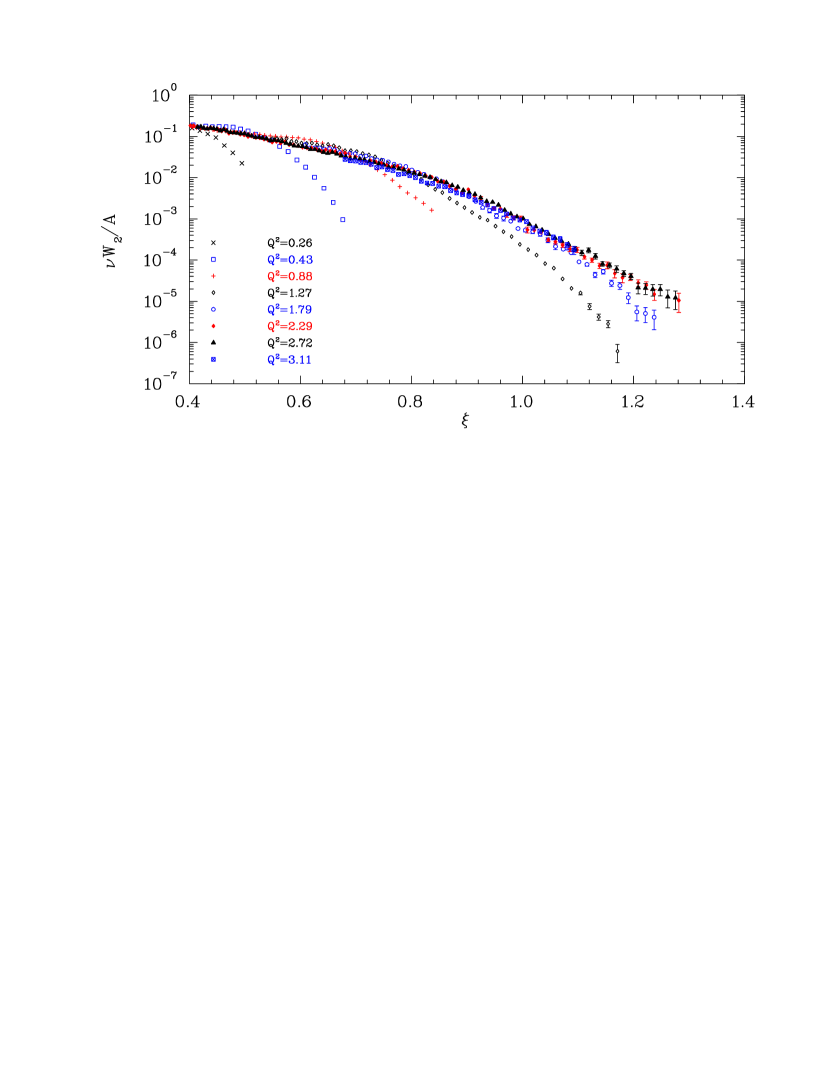
Figure 1.7: Structure function $\nu W_{2}$ vs. $\xi$ for Iron from SLAC experiment NE3. The different curves represent different values of beam energy and spectrometer angle and are labeled by the value of $Q^{2}$ at $x=1$. Errors shown are statistical only

While the previous data shows indications of scaling in both $y$ and $\xi$, the coverage in $Q^{2}$ limits the amount of information that can be extracted. In order to have a clear sign of a scaling behavior, we need to observe that the scaling function remains flat over a large range of $Q^{2}$. For the $y$-scaling, final-state interactions are expected to be small only for the large $Q^{2}$, and may not yet be completely negligible in the range of the NE3 data. In addition, the structure function appears to be scaling in $\xi$ only for low values of $\xi$ or at the highest values of $Q^{2}$. It has been suggested by Benhar and Luiti [37] that the observed scaling in $\xi$ is a combination of the normal inelastic scaling for low $\xi$, and a modified version of $y$-scaling in the high-$\xi$ region, arising from an accidental cancellation of $Q^{2}$ dependent terms coming from the transformation from $y$ to $\xi$ and terms coming from the shrinking final-state interactions. They predict that this accidental (but imperfect) cancellation will continue to higher $Q^{2}$ values, and that $\xi$-scaling violations at the level seen in the previous data will continue to much higher momentum transfer (up to $Q^{2}\sim 10$ (GeV/c)²).

The purpose of experiment e89-008 is to extend significantly the coverage in both $x$ and $Q^{2}$. This will allow us to better examine the scaling of the quasielastic scattering, to more precisely examine the transition from quasielastic to inelastic scattering at large $Q^{2}$, and to study the observed scaling in $\xi$ in the transition region. Improved data in the quasielastic region may be used to extract the momentum distribution of the nucleons in the nucleus. Going to higher $Q^{2}$ improves the coverage in $y$, and reduces the final-state interactions, reducing the uncertainty in the extracted momentum distribution. Improved measurements of the structure function can be used to examine the quark momentum distributions in the nucleus, in particular at large $x$, and can be used to examine the observed $\xi$-scaling over a larger range of momentum transfers in order to better understand the cause of the scaling behavior.

Chapter 2 Experimental Apparatus

2.1 Overview

Experiment e89-008, “Inclusive Scattering from Nuclei at $x>1$ and High $Q^{2}$”, was run at CEBAF (now called Jefferson Lab) in the summer of 1996. CEBAF was designed to provide a high current, 100% duty factor beam of up to 4 GeV to three independent experimental halls. During the running of the experiment, Hall C was the only operational experimental area. Data was taken simultaneously in the High Momentum Spectrometer (HMS) and the Short Orbit Spectrometer (SOS). Inclusive electron scattering from Deuterium, Carbon, Iron, and Gold was measured with 4.045 GeV incident electrons over a wide range of angles and energies of the scattered electron. Data from Hydrogen was taken for calibration and normalization.

2.2 Accelerator

During the running for e89-008, CEBAF provided an unpolarized, CW electron beam of 4.045 GeV, with currents of up to 80 $\mu$A. A schematic of the accelerator is shown in figure 2.1. The electron beam is accelerated to 45 MeV in the injector. It then passes through the north linac and is accelerated an additional 400 MeV by superconducting radio frequency cavities. The beam is steered through the east arc, and passes through another superconducting linac, gaining another 400 MeV. At this point, the beam can be extracted into any one of the three experimental halls, or can be sent through the west arc for additional acceleration in the linacs, up to 5 passes through the accelerator. For each pass through the accelerator, the electron beam gains 800 MeV, for a maximum beam energy of 4.045 GeV. The linacs can be set to provide less than 800 MeV per pass, but the energy of the extracted beam is always a multiple of the combined linac energies, plus the initial injector energy.

The beams from different passes through the machine lie on top of one another. Because they are different energies, they require different bending fields in the arcs. Therefore, the west arc has five separate arcs, and the east arc has four, each set to bend a beam of a different energy. The beams are separated at the end of each linac, transported through the appropriate arc, and recombined before passing through the next linac. At the end of the south linac, after the beam of different energies are split, the beams can be sent for another pass through the accelerator or they can be sent to the Beam Switch Yard (BSY). At the BSY, the beam can be delivered into any of the three experimental halls.

Figure 2.1: Overhead schematic view of the Accelerator and Experimental Halls.

The beam has a microstructure that consists of short (1.67 ps) bursts of beam coming at 1497 MHz. Each hall receives one third of these bursts, giving a pulse train of 499 MHz in each hall. The Beam Switch Yard takes the beam that has been extracted from the accelerator and sends the pulses to the individual halls. Beams of different energies can be simultaneously delivered into the three experimental halls.

The beam has an emittance of $\sim$2x10^-9 mrad at 1 GeV (4$\sigma$ value), and a somewhat lower value at higher energies. The fractional energy spread is $<$10^-4. The relative beam energy can be measured with a fractional uncertainty of $10^{-4}$ and is known absolutely to better than $10^{-3}$. The nominal beam energy is determined from the magnet settings in the arcs in the accelerator or in the Hall C Arc. The beam energy can be measured by fixing the magnet settings in the Hall C Arc and measuring the beam position at the beginning, middle, and end of the arc in order to accurately measure the path length of the beam through the arc. By measuring the path of the electron beam and using precise field maps of the arc magnets, the field integral, $\int B\cdot dl$, through the arc is measured accurately, and this is used to determine the energy of the beam. For one and two pass beams, the energies measured in the arcs have been checked by measuring the differential recoil from a composite target, and by measuring the diffractive minimum in scattering from the Carbon ground state (See section 2.3.3).

2.3 Hall C Arc and Beamline

After the electron beam has been accelerated to the desired energy in the main accelerator, it can be delivered into one or more of the three experimental halls. The beam is split at the end of the accelerator, and beam for Hall C is sent through the Hall C arc and into the end station. The arc is equipped with a variety of magnets used to focus and steer the beam, as well as several monitors to measure the energy, current, position, and profile of the beam. Figures 2.2 and 2.3 show the hardware in the Hall C Arc and Hall C beamline.

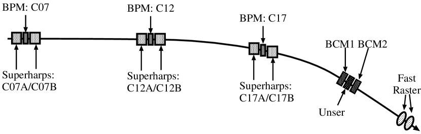
Figure 2.2: Hardware in the Hall C Arc (not to scale).

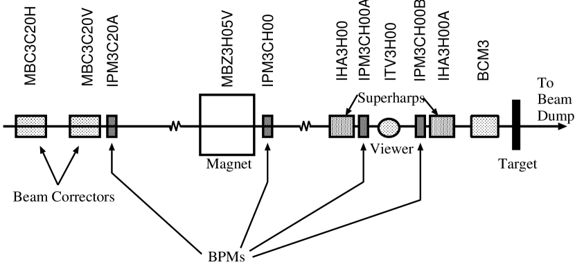
Figure 2.3: Hardware in the Hall C beamline (not to scale).

2.3.1 Beam Position/Profile Measurements

Several harps and superharps are used to measure the beam profile. A harp consists of a frame with three wires, two vertical wires that measure the horizontal beam profile and one horizontal wire that measures the vertical beam profile. An Analog-to-Digital Converter (ADC) measures the signal on the wires and a position encoder measures the position of the ladder as they pass through the beam (see fig 2.4). Using the position information and the ADC measurements, the position and profile of the beam can be measured. Several harps are located throughout the accelerator for use in monitoring the position and shape of the beam. The superharps are essentially the same as the harps, but they have been more accurately fiducialized and surveyed for absolute position measurements. The superharps are primarily used for the beam energy measurement in the Hall C arc. Three superharps are located on aligned granite tables at the beginning, middle, and end of the Hall C Arc. Using the positions measured by the three superharps along with the field maps of the arc bending magnets, the beam energy and emittance can be determined. The absolute beam energy can be determined with a fractional uncertainty of $\sim$2x$10^{-4}$ with this method and beam energy changes below the $10^{-4}$ level can be measured. During data taking, beam energy changes are monitored with the BPMs in the arc. Details of the superharp construction and operation can be found in [38].

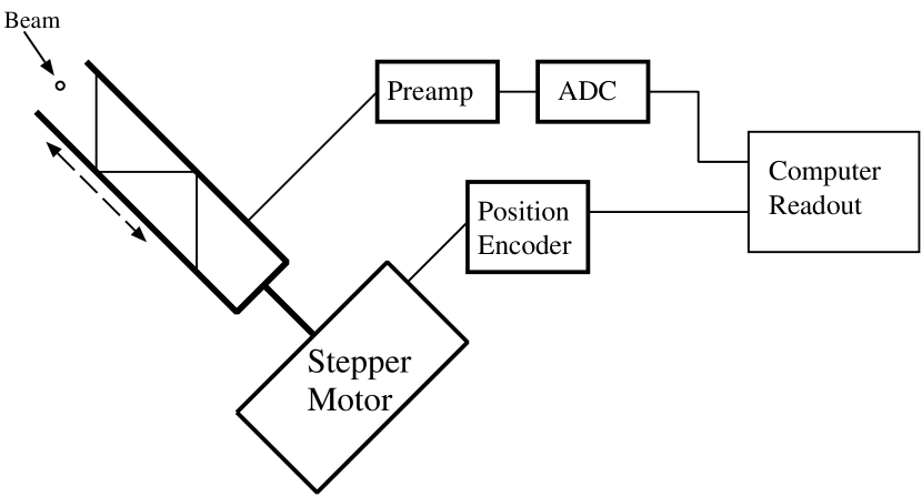
Figure 2.4: Schematic of the harp and superharp systems.

2.3.2 Beam Position Monitors

The position of the beam in Hall C was monitored using four beam position monitors (BPMs). The BPMs are described in detail in [39]. Each BPM is a cavity with four antennae rotated $\pm 45^{\circ}$ from the horizontal and vertical. Each antenna picks up a signal from the fundamental frequency of the beam which is proportional to the distance from the antenna. The beam position is then the difference over the sum of the properly normalized signals from two antennae on opposite sides of the beam. Because the position is determined by the ratio of signals in the antennae, the position measurement is independent of beam current. Non-linearity in the electronics can introduce a small current dependence in the BPM readout. For the range of currents used during e89-008, this led to an uncertainty of $<$0.5 mm. From these four antennae, the relative $(X,Y)$ position of the beam can be determined once the signals from the four antennae have been properly calibrated. The beam position from the BPMs in the arc were compared to the Arc C superharps in order to calibrate the absolute position for the BPMs. The final accuracy of the beam position measurement was $\pm 1.0$ mm, with a relative position uncertainty of 0.1-0.2 mm (neglecting the current dependence). The BPMs in the Hall C beamline were not calibrated against the superharps. The calibration of the BPMs was fixed at a nominal value, and the beam was steered so that x=1.8 mm, y=-1.0 mm at the final BPM. This was determined to be the correct position at the target based on requiring mid-plane symmetry in both spectrometers. This position was verified by placing a sheet of Plexiglas at the front of the scattering chamber and determining the beam position at the target from the position of the darkened spot on the Plexiglas.

2.3.3 Beam Energy Measurements

There are two main ways to measure the beam energy. During e89-008 data taking, the nominal beam energy was determined by examining the settings of the magnets in the east arc. The east arc is a 180 degree bend, and so knowing the fields in the magnets allows one to determine the energy of the beam. However, the path length variations, uncertainty in the field integral, and the large ($0.2-0.3\%$) energy acceptance of the arc limit the measurement (relative and absolute) to $\sim 10^{-3}$.

A more precise measurement of the beam comes from the settings of the magnets in the Hall C Arc. This is not done continuously, because the focusing elements in the arc are turned off for the measurement and the superharps are used to scan the beam, following the procedure of [40]. Using the superharps to measure the beam position at the beginning, middle, and end of the arc, the beam is steered to insure that it follows the central trajectory, with all corrector magnets turned off. One of the dipoles in the arc (the ‘golden’ magnet) has been precisely field mapped. The other dipoles are assumed to have the same field map, normalized to the central field value. With the precise knowledge of the field, and the absolute beam positions measured with the superharps, the field integral is well known, and the beam energy can be determined with an uncertainty of $\delta p/p\approx 2\times 10^{-4}$. Details of the energy measurement and associated uncertainties can be found in ref. [41]. However, after the analysis of the Arc measurements was completed, it was discovered that the degaussing procedure used for the Arc dipoles during the measurements was not the same as was used when the dipole fields were measured. The energy measurements assume that the dipole is run to 300 Amps, and then reduced to the desired current value. During data taking, the dipoles were only being ramped up to 225 Amps. This led to a difference in residual field which led to an overestimate of the beam energy. Figure 2.5 shows the residual field versus beam energy for both degaussing procedures, and the correction this implies for the Hall C Arc measurement of the beam energy. The energy we use in the data analysis and in comparisons to other beam energy measurements has been corrected for this effect based on the bottom curve. An additional uncertainty has been applied for this correction (0.01% for energies below 3 GeV, 0.02% for higher energies).

Figure 2.5: Residual field for both Arc dipole degaussing procedures and the error induced in the calculated beam energy. The top figure shows the residual field as a function of beam energy for the two different degaussing procedures. The bottom figure shows the correction to the beam energy caused by using the 225 Amp degaussing for the Arc measurement, but the 300 Amp procedure for the magnet mapping.

The BPMs can be used to monitor the beam energy when data taking is in progress. However, because the position is not measured as well with the BPMs as the superharps, and because the corrector magnets are energized, total integrated field ($\int B\cdot dl$) is only known to $\sim$0.2%. This limits the accuracy of the the absolute beam energy measurement to $0.2-0.3\%$ of the beam energy. However, relative beam energy changes can be detected at the $2-3\times 10^{-4}$ level.

In addition to measuring the beam energy by using dipole magnets in the accelerator, the energy has been measured using three different schemes that are independent of the knowledge of the dipole fields. These measurements are described in detail in ref. [42]. The results of the measurements are summarized in table 2.1, and compared to the beam energy measured in the Hall C Arc.

Nominal	Method	EBeam	EArc
		(MeV)	(MeV)
	Differential
845.0	Recoil method	844.7$\pm$1.5	844.56$\pm$0.19
	Diffractive
845.0	Minima method	844.7$\pm$0.9	844.56$\pm$0.19
	Diffractive
845.0	Minima method	845.1$\pm$0.9	844.56$\pm$0.19
	Diffractive
1645.0	Minima (elastic)	1645.3$\pm$2.8	1648.5$\pm$0.5
2445.0	Elastic H(e,e’p)
		2444.9$\pm$5.0	2449.9$\pm$0.6
4045.0	H(e,e’)
	Elastic Scan	4038.9$\pm$1.8	4036.1$\pm$0.6

Table 2.1: Summary of the beam energy measurements. Arc measurements are corrected for hysteresis error.

The first scheme is the differential recoil method. This relies on determining the beam energy by measuring the difference in recoil energy between elastic scattering from light and heavy nuclei. Using a composite target (BeO), the elastic scattering from Beryllium and Oxygen are measured simultaneously, and the difference in recoil energy is used to determine the beam energy. The recoil energy for elastic scattering from a nucleus with mass M is:

$$E_{recoil}=Q^{2}/2M=(2EE^{\prime}/M)\sin^{2}{\theta/2}.$$ (2.1)

For a composite target, the energy difference is:

$$\Delta E_{recoil}=2E\sin^{2}{\theta/2}(E_{1}^{\prime}/M_{1}-E_{2}^{\prime}/M_{2})\approx 2EE^{\prime}\sin^{2}{\theta/2}(1/M_{1}-1/M_{2}).$$ (2.2)

The uncertainty in this procedure comes from the uncertainties in measuring the recoil energy and scattering angles. This method was used to measure the energy with 1 pass beam (nominally 845 MeV). The energy measured was 844.7$\pm$1.5 MeV, with the uncertainty dominated by uncertainty in the determination of the centroids of the detected peaks. This method was not used at higher energies because of the drop in the rate of elastic scattering as the beam energy increases and the loss of energy resolution, which makes it difficult to measure the energy difference precisely.

The second method involves comparing the cross section from elastic scattering from Carbon and inelastic scattering to the first excited state. The ratio of these two cross sections has a minimum at $Q^{2}=0.129(GeV/c)^{2}$ [43], as seen in figure 2.6. The minimum occurs in the elastic cross section, but by taking the ratio to the first excited state, systematic uncertainties in locating the position of the minimum are reduced. Uncertainties come from determining the minimum of the ratio of the cross sections and uncertainty in the scattering angle. In order to improve the determination of the minimum, the ratio of cross sections was compared to a ratio taken from a model of the cross sections, and the shape of the ratio near the minimum was fit to the model ratio. This method was used to measure the beam energy for a one-pass beam, and gave a value of 844.7$\pm$0.9 MeV, with the uncertainty dominated by the uncertainty in the position of the minimum. Data was also taken with a two-pass beam, but the model used for the excited state scattering failed at these energies. However, a measurement of the beam energy was made (with larger systematic uncertainties) by comparing the measured ground state cross section to the model ground state cross section. The energy was determined to be 1645.3$\pm$2.8 MeV. At higher energies, the reduction in cross section and energy resolution make it difficult to find the minimum, and this technique is not useful for beam energy measurements above $\sim$2 GeV.

The beam energy can also be determined by measuring elastic H(e,e’p) scattering. By measuring the angle and momentum of both the scattered electron and proton, the initial electron energy can be determined. This method is not as accurate as the previous methods, due primarily to the uncertainty in the momentum of the detected proton and electron. However, it can be used at all energies, while the previous methods are only possible for one- and two- pass beam. For one- and two- pass energies, the uncertainty from this method is significantly larger than for the previous methods. For three-pass beam, the measured energy was 2445.0+4.7-4.9 MeV.

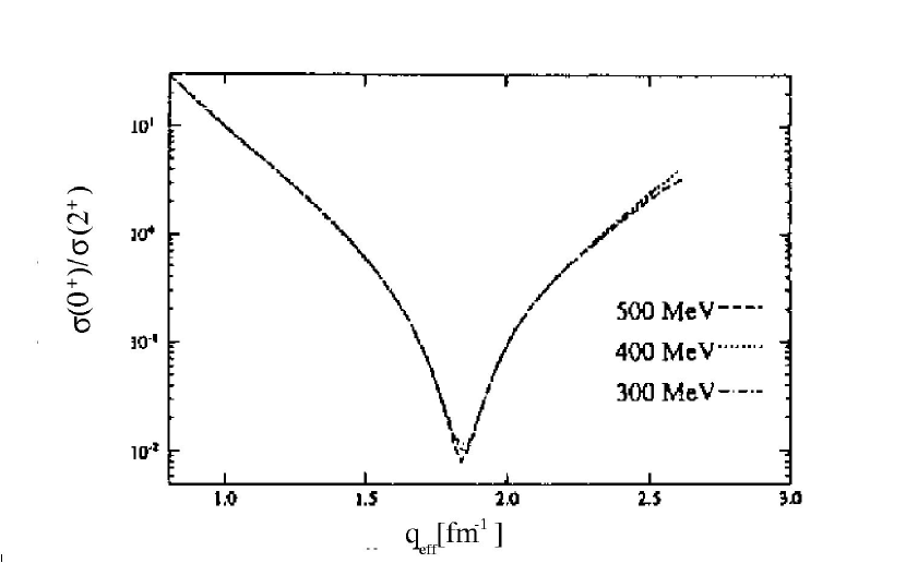
Figure 2.6: Ratio of scattering into ground state vs first excited state of Carbon as a function of $q$.

Unfortunately, none of these methods work well for 4 GeV beam. A measurement was made by taking single arm H(e,e’) elastic scattering data between 20^∘ and 60^∘. If the spectrometer momentum and angle are perfectly well known, then the measurement of $W^{2}$ at any of the measured angles can be used to determine the beam energy. If the angle and momentum are not well known, an inclusive measurement at a single angle cannot distinguish a beam energy offset from a spectrometer angle or momentum offset. However, as long as the beam energy is fixed, the angular dependence of the position of the $W^{2}$ peak for elastic scattering can be used to determine beam energy and spectrometer momentum offsets. Figure 2.7 shows the fractional energy offset, $\Delta E/E$, necessary to center the elastic peak at $W^{2}=M_{p}^{2}$ for each momentum. The slope indicates a momentum offset in the spectrometer, while the overall offset indicates a beam energy offset from the nominal value (4.045 GeV for this scan). The conclusion from the scan was that the beam energy was $\sim$0.15% below the nominal energy, with a $\pm$0.04% uncertainty, giving a beam energy measurement of 4038.9$\pm$1.8 MeV. This is to be compared to the Arc measurement of 4036.1$\pm$0.6 taken at the same time. The measurement of the beam energy and spectrometer momentum from the elastic measurements is described in detail in section 2.5.3. This technique was not used during e89-008. Elastic measurements were taken at a variety of angles, but they were taken at different times during the run. During our run, there were beam energy drifts at the 0.03% level (see below). Because the beam energy was not identical for the different elastic measurements, this technique was not used to directly measure the beam energy or constrain the spectrometer momentum offset.

Figure 2.7: Error in position of elastic peak (as $\Delta E/E$) as a function of detected momentum for the HMS elastic scan.

Figure 2.8: Comparison of the beam energy measurements using kinematic methods to the Arc measurements. $\Delta E/E=(E_{meas}-E_{Arc})/E_{Arc}$. Errors shown include uncertainty in both measurements. The kinematic methods give beam energies consistent with the Arc measurements, and provide and independent verification of the Arc measurements, with a 0.36% uncertainty.

Figure 2.8 shows the difference between the Arc energy measurements and the measurements from the kinematic methods from table 2.1. The measurements are consistent with the Arc measurement, and provide an independent verification of the uncertainty in the Arc measurement. Combining the measurements at different energies, we verify the Arc measurement with a 0.36% uncertainty. For e89-008, the beam energy as measured by the Arc was 4046.1$\pm$0.6 MeV. However, while the Arc measurement gave a 0.6 MeV uncertainty (0.015%), the beam energy varied somewhat during the run due to occasional drifting and rephasing of the superconducting cavities, and this is the most significant source of uncertainty in the beam energy. The BPMs in the Hall C arc are used during the run to monitor relative energy changes, and indicate that the beam energy varied at the level of $\pm$0.03% during the course of the run. Because the tune through the Arc was not optimal during e89-008, we did not try to use the Arc BPM information to correct the beam energy on a run-by-run basis. Therefore, we used a fixed beam energy in the analysis and assumed a 0.03% uncertainty. The Arc measurement was taken at the very end of the run, and the Arc BPMs for the previous runs indicated that the Beam energy was higher than the average during that period. Therefore, we used the nominal beam energy, 4045.0 MeV, with an uncertainty of 1.2 MeV (0.03%) based on the beam energy variations during the run. The beam energy spread is $<$1x10^-4, and has a negligible effect on the measured cross section compared to the uncertainty in the central value of the beam energy.

The kinematic beam energy determinations provide independent measurements of the beam energy, and are useful in determining the uncertainty in the absolute beam energy measurement from the Hall C Arc. However, none of these procedures were used during e89-008. The only measurements that are useful for 4.045 GeV beam are the elastic measurements. Because e89-008 took only single-arm data, the H(e,e’p) method could not be used. However, inclusive elastic data was taken at each angle. The elastic data was taken at different times during the run, and so the the shift in $W^{2}$ is now a combination of the beam energy offset, the spectrometer angle and momentum offsets, and a time-dependent beam energy drift. We use the previous measurements to set the uncertainty for the Arc measurement and use the scan to check the spectrometer angle and momentum offset. The elastic data taken during e89-008 indicates that the spectrometer offsets were consistent with the known beam energy variations and the angle/momentum offsets determined from previous data (section 2.5.3).

2.3.4 Beam Current Monitors

The beam current in the hall was measured with three microwave cavity beam current monitors (BCMs). The current is monitored by using the beam to excite resonant modes in cylindrical wave guides (the BCMs). The wave guides contain wire loop antennas which couple to resonant modes. The signal is proportional to the beam current for all resonant modes. For certain modes (e.g. the $TM_{010}$ mode), the signal is relatively insensitive to beam position. By choosing the size of the cavity, one can choose the frequency of the $TM_{010}$ mode to be identical to the accelerator RF frequency in order to make the cavity sensitive to this mode. The material and length can be varied to vary the quality factor, the ratio of stored energy to dissipated power, weighted by the resonant frequency, $Q=\omega_{0}W/P_{d}$. The cavities and associated readout electronics as used during e89-008 are described in [44, 45]

Temperature changes can cause expansion or contraction of the cavity. This leads to a modification of the frequency of the $TM_{010}$ mode and a detuning of the cavity away from the desired 1497 MHz. Therefore, as the temperature changes, the measured power decreases, giving an error in the current measurement. If the temperature is within 2 degrees of the tuning temperature, then the temperature dependence in the current measurement is proportional to $2Q\alpha\Delta T$ for small temperature variations ($\alpha$ is the thermal coefficient of expansion of the cavity, $\Delta R=\alpha R\Delta T$). This leads to a modest temperature dependence, $\approx 0.25\%/$degree C. However, if the operating temperature is several degrees away from the tuning temperature ($\sim$5 degrees), then the temperature dependence is greatly increased, and the error in the measured current is $\approx$1.5%/degree. Because of this large temperature dependence, $Q$ was reduced by a factor of three from its initial value in order to minimize the temperature variation of the output. During e89-008, the temperature of the cavity was stable $\pm$0.2 C, and was less than 1 C from the tuning temperature, giving negligible ($<0.05\%$) errors on the current measurement. In addition, the temperature of the readout electronics can lead to an error in the charge measurement. For BCM1, the temperature coefficient was $\sim 0.3\%/\Delta T$, and for BCM2 (the primary BCM for e89-008) it was somewhat better. However, the electronics room temperature was stabilized to $\pm 0.5$ C, leading to uncertainties below the 0.2% level.

In addition to the microwave cavity BCMs, there is also a parametric DC current transformer (Unser monitor [46]) that measures the beam current. The Unser monitor has a very stable and well measured gain, but can have large drifts in its offset. Therefore, it is not used in the experiment to determine the accumulated charge. However, because the gain is stable, the Unser monitor is used to calibrate the gain of the microwave cavity BCMs. Calibration runs were taken about once a day in which the beam was alternately turned off and on over 2 minute intervals. During the beam off periods, the offsets of the Unser and cavity monitors were measured. During the beam on periods, the gains of the cavity monitors were calibrated using the known gain and measured offset of the Unser. The Unser gain was calibrated before the experiment by sending a precisely measured current through a wire running along the inside of the cavity. Analysis of all of the calibration runs indicated that the offsets and gains were stable during the experiment. A single gain (and offset) was determined for each BCM and that value was used throughout the run. The charge measurement was stable to within 0.5%, and the overall uncertainty on the absolute charge for each run was 1.0%.

2.3.5 Beam Rastering System

The electron beam generated at CEBAF is a high current beam, with a very small transverse size ($\mathrel{\raise 1.29167pt\hbox{$<$}\mkern-14.0mu\lower 2.58334pt\hbox{$\sim$}}$200 $\mu$m FWHM). There are two rastering systems designed to increase the effective beam size in order to prevent damage to the target or the beam dump. The fast raster system, 25 meters upstream of the target, is designed to prevent damage to the solid targets and to prevent local boiling in the cryogenic targets. The slow raster system is situated just upstream of the target, and is designed to protect the beam dump. During e89-008, the increase of the beam size caused by multiple scattering in the scattering chamber exit window and the Helium bag was enough to prevent damage to the beam dump without the slow raster, so it was not in use during data taking. Currents above 80$\mu$A would have required the slow raster.

The fast raster system consists of two sets of steering magnets. The first set rasters the beam vertically, and the second rasters the beam horizontally. The current driving the magnets was varied sinusoidally, at 17.0 kHz in the vertical direction, and 24.2 kHz in the horizontal direction. The frequencies were chosen to be different so that the beam motion would not form a stable figure at the target. Instead, it moves over a square area, $\sim 2.4$mm across. The rastering was sinusoidal, and so the average intensity was greatest around the edges of the box, since this is where the beam is moving most slowly (see figure 2.9). Because the beam spends $\sim 40\%$ of the time in the outermost 0.1-0.2mm of the box, the peak power density decreases more slowly than the inverse of the area of the raster pattern. However, the reduction of power density was sufficient to prevent any significant density fluctuations due to local boiling in the cryogenic targets for the currents used in this experiment.

Figure 2.9: Beam profile with the fast raster in operation. The plot shows the readback of the fast raster currents (which correspond to $x$ and $y$ position at the target) for each event, giving the beam intensity distribution. For normal data taking, the raster size was set to $\pm$1.2 mm in both $x$ and $y$.

2.3.6 Scattering Chamber

The Hall C scattering chamber is a large cylinder, 123.2 cm inner diameter, 136.5 cm high, with 6.35 cm Al walls. The cylinder has cutouts for the two spectrometers, large enough to cover the full angular acceptances of the HMS and SOS, for both in-plane and out-of-plane (up to $20^{\circ}$) operation of the SOS. In addition, there are entrance and exit openings for the beam as well as a pumping port and several viewing ports. The beamline connects directly to the scattering chamber, so the beam does not pass through any entrance window. The beam exit window consists of a Titanium foil, approximately 60 mg/cm² thick. The HMS cutout is 20.32 cm tall and covered with an Aluminum window 0.04064 cm thick. The SOS port is 32.258 cm tall and covered with a 0.02032 cm thick Al window. The chamber is mounted on a bottom plane which mounts to the fixed pivot in the hall. The top plate contains openings through which the cryotarget plumbing and lifting mechanisms and the solid target system are inserted. The solid target ladder can be lifted out of the scattering chamber, and the chamber sealed off. The solid target ladder can then be replaced or repaired without breaking the scattering chamber vacuum. The scattering chamber must be opened up in order to change the cryogenic targets, which requires breaking vacuum.

2.3.7 Exit Beamline

There is a beamline for the last 25 m before the beam dump, but there is no beamline between the exit of the scattering chamber and the dump line. In order to reduce background from electrons interacting with the air, a temporary helium-filled beamline was installed between the scattering chamber and the dump line. The beamline was made from Aluminum and was approximately 24m long. It was a circular pipe with four segments. The segments were small near the scattering chamber in order to avoid interfering with the spectrometers, and became larger as they approached the beam dump vacuum line. The first piece was 5.1cm in diameter, the 2nd was 15.2 cm, the third was 30.5 cm, and the final piece was 45.7 cm diameter. The entrance and exit windows to the temporary beamline were 0.406 mm Aluminum.

2.4 Targets

The scattering chamber has room for two target ladders, one for cryogenic targets and one for solid targets. In order to use the solid targets, the cryotarget ladder must be lifted fully out of the beam and rotated $90^{\circ}$ so that it is out of the beam path and does not interfere with the spectrometer acceptances. Then, the solid target ladder can be inserted.

2.4.1 Cryotarget

The standard cryotarget ladder contains three pairs of target cells with one short cell ($\sim$4 cm) and one long cell ($\sim$15 cm) per pair. For this experiment, we had cryogenic Hydrogen and Deuterium targets, a pair of empty cells, and a pair of dummy cells used for measuring background from the aluminum target cell walls. The dummy cells consisted of two flat aluminum targets, placed at the same positions as the endcaps of the cryotarget cells, but with walls approximately 10 times thicker. This allows us to measure the background from the aluminum endcaps very rapidly, and makes the total thickness (in radiation lengths) of the dummy cells close to that of the full targets. Figure 2.10 shows the arrangement of the full cryotarget ladder. A complete description of the Hall C cryogenic target system can be found in ref. [47].

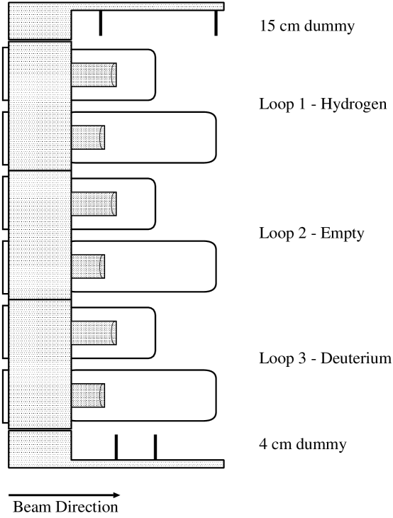
Figure 2.10: Side view of the full cryotarget ladder.

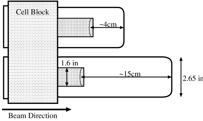
Figure 2.11: Side view of one cryotarget loop.

The cryotarget system has three separate loops (for Hydrogen, Deuterium, and Helium targets), with each loop linked to a short and long target cell. Figure 2.11 shows a side view of the two cells attached to a single target loop. Each loop consists of a circulation fan, a target cell, heat exchangers and high and low powered heaters. The target can dissipate in excess of 200 Watts of power deposited by the electron beam. In the loops, an axial fan inside a heat exchanger forces the target liquid to flow through two cells on an aluminum cell block, which is connected to the heat exchanger. Extending from each cell block are two target cells. The cells are thin aluminum cylinders made from beer can stock, 6.731 cm in diameter, with 0.0178 cm walls. The target liquid flows through these cells. Inside of the large cells are smaller aluminum flasks. The entrance and exit endcaps are both curved slightly, which gives a thickness variation with beam position. The maximum target length change for a 2mm beam offset is less than 0.5% for the 4cm cells, and $\sim$0.1% for the 15cm cells. During the cryotarget running, the beam position was typically kept within 1-2mm of the nominal central position, with an average offset of less than 1mm (better than 0.5 mm for all of the elastic runs). The heat exchanger has approximately 3.5 grams/second of 4 K liquid helium flowing through the refrigerant side, and provides the cooling for the target liquids. The cold helium is provided by the CEBAF End Station Refrigerator, and is returned at $\sim$21.5 K. High power heaters are used to maintain a constant heat load for the system, so that the cooling power stays constant as the beam current changes. There is sufficient cooling power to keep the heaters running on multiple cells. This meant that two cells (one hydrogen and one deuterium) could be kept ready for beam, eliminating delays caused when one loop needs to be powered down before another can be powered up. Low power heaters maintain the cryotargets at their operating temperatures, and correct for small fluctuations in the beam current. The hydrogen target is operated at $\sim$0.2MPa (29 PSIA) pressure, and a temperature of 19K. In this state, the boiling temperature of hydrogen is 22.8K. The deuterium target is also operated in a subcooled fashion, at 22K. Table 2.2 lists the targets available in the cryotarget ladder for e89-008.

Target	$t_{target}$	$t_{cryogen}$	$t_{Al}$	Total Radiation
	(cm)	(g/cm2)	(g/cm2)	Length (%)
LH2	4.36	0.3152	0.0565	0.748
LH2	15.34	1.1091	0.0516	2.024
LD2	4.17	0.6964	0.0502	0.776
LD2	15.12	2.5250	0.0559	2.292
Dummy	4.01	-	0.5215	2.162
Dummy	15.0	-	0.5216	2.163

Table 2.2: Cryogenic target densities.

The loops are connected to a vertical lifting mechanism, which lifts the target ladder in order to place the desired cell in the beam. In addition, if the ladder is lifted to its highest position, the entire assembly can be rotated out of the beam by 90^∘. This allows the insertion of the solid target ladder and keeps the cryotarget cells and lifting mechanism clear of the spectrometer acceptances.

The temperature of the target cryogen is determined by a resistance measurement of two Lakeshore Cernox resistors for each loop, and the absolute temperature is measured to an accuracy of $\sim$100mK. Changes in the temperature are measured with 50mK accuracy. The density dependence on temperature is $\frac{1}{\rho}\frac{d\rho}{dT}=-1.25\%/K$, leading to an an uncertainty in density of less than 0.2%. Pressure changes have a much smaller effect on the density, $\frac{1}{\rho}\frac{d\rho}{dP}=0.01\%/PSIA$, and were negligible in the final density uncertainty. The overall uncertainty in the calculation of the density (without beam) is $\sim$0.4%, mainly due to the uncertainty in the relative amounts of ortho and para hydrogen and the uncertainty in the equation of state. The length of the target cells has been corrected for thermal contraction ($\sim$0.4% at the operating temperatures, and a 0.2% uncertainty is assumed for this correction. The uncertainties in the target thicknesses are summarized in table 2.3.

The density of the hydrogen is 0.07230(36) g/cm³ at the operating temperature of 19K. The deuterium has a density of 0.1670(8) g/cm³ at 22K. There is an additional current-dependent uncertainty in the density due to local target boiling. The analysis of the density dependence for runs up to August 1996 is described in [48]. Figure 2.12 shows the normalized yield (events per charge) for the 15 cm cryogenic deuterium target taken at the end of the experiment. During e89-008 data taking, the cryogenic targets were run at or below 55 $\mu$A, with a $\pm$1.2 mm beam raster. For this current and raster size, there is no significant loss of target density. However, it was discovered after e89-008 that the beam tune into Hall C was not perfect, and that the unrastered beam size was larger than the desired 80-100$\mu$m [49]. In later runs, the tune was improved and the spot size reduced. Because the raster motion is sinusoidal in $x$ and $y$, the beam spends a large fraction of the total time near the edges of the raster pattern (see figure 2.9). Therefore, the intrinsic size of the beam is still important when determining localized boiling. For the runs where the beam tune was improved, there was a density loss of $\sim$0.04%/mm/$\mu$A. This would correspond to a density loss of 1.8% at 55 $\mu$A with a 1.2mm raster. Our typical beam cross section was $\sim$3 times larger then for the improved tune, and was always $\mathrel{\raise 1.29167pt\hbox{$>$}\mkern-14.0mu\lower 2.58334pt\hbox{$\sim$}}$2 times larger. While the beam spot may not have been small enough during e89-008 to have as large of an effect as seen with the improved beam tune, we cannot be sure that the spot size was completely stable during the run. This means that the effect of localized target boiling during data taking could have been larger or smaller than the effect measured during our test run. Therefore, we apply no correction to the density for target boiling, but assign an uncertainty of $0.013\%/mm/\mu$A (one third of the measured effect for the improved tune) to our target density, corresponding to a 0.6% uncertainty at 55 $\mu$A.

Figure 2.12: Rate versus current for cryogenic targets. The different symbols represent different rastering sizes for the beam. At the highest currents, there is a reduction in rate due to localized boiling of the target.

Target	LH4	LH15	LD4	LD15
Beam position at target	0.1%	0.0%	0.2%	0.1%
$d\rho/dT$	0.2%	0.2%	0.2%	0.2%
$dL/dT$	0.2%	0.2%	0.2%	0.2%
$\rho_{calc}$	0.4%	0.4%	0.4%	0.4%
target purity	$<$0.1%	$<$0.1%	0.2%	0.2%
Total (without beam)	0.50%	0.49%	0.57%	0.54%
Local boiling (10-55$\mu$A)	0.1-0.6%	0.1-0.6%	0.1-0.6%	0.1-0.6%
Total	0.5-0.8%	0.5-0.8%	0.6-0.8%	0.6-0.8%

Table 2.3: Uncertainties in the thickness of the cryogenic targets.

Samples of the gases used to fill the targets were taken in order to measure the purity of the cryotargets. For the hydrogen gas used during e89-008, the target was 99.8% Hydrogen, and this was corrected for in the elastic analysis. The quantity of impurities (Nitrogen and Oxygen) was small enough that the background to the elastic measurement is negligible. For the deuterium, the gas was 99.6% Deuterium by number of nuclei, 99.2% by mass.

2.4.2 Solid targets

The solid target ladder is water cooled and has space for three thin targets and two thick targets (see figure 2.13). Two Carbon, two Iron, and one Gold target were used during the experiment (see table 2.4). The target was cooled by flowing water through a copper tube that was attached to the back of the target. The tube was shaped so that water flowed past each target on all four sides. In addition to the physics targets, a Beryllium-Oxide (BeO) target was attached to the bottom of the ladder. It did not need to be water cooled because it was only used for beam tuning. At low currents, the beam spot is visible on the BeO target, and the the spot can be used to determine the position of the beam at the target. At higher current, the spot is visible on all of the targets. The ladder can be rotated so that the spectrometers can have a clear view of the target, without interference from the sides of the target frame. The targets were approximately 3.0 cm high and 4.2 cm wide, but when clamped into the frame, the area visible to the beam was 2.0 cm by 3.3 cm.

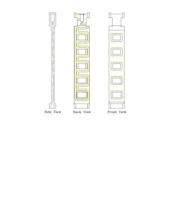
Figure 2.13: The e89-008 solid target ladder. The bottom two slots are deep enough to hold thick (Carbon) targets. The BeO target (not shown) was hung from the bottom of the ladder. The shaded region on the back view shows the copper tubes that carry the cooling water.

Target	Thickness	Thickness	$\delta t/t$
	(radiation lengths)	(mg/cm2)
C	2.09%	.8915(12)	0.5%
C	5.88%	2.510(10)	0.5%
Fe	1.54%	.2129(3)	1.0%
Fe	5.84%	.8034(11)	2.0%
Au	5.83%	.3768(6)	1.0%

Table 2.4: Solid target thicknesses. All targets contained natural isotopic abundances.

The beam has a roughly gaussian distribution, with a width of about 200$\mu$m, and so the size of the beam spot on the target is determined by the raster size ($\pm$1.2mm horizontally and vertically for e89-008). The maximum beam position deviations were less than 4 mm, so there was always at least 5 mm clearance from the frame of the target ladder. This was sufficient to insure that there was no problem with background from the halo of the beam striking the frame. Since the beam profile monitors can only measure the profile of the beam where the intensity is relatively large, we took some test runs with the beam 1mm to 4mm away from the BeO target in order to look for non-gaussian tails to the beam profile. The test gave a crude measurement of the beam width which was consistent with the 200 $\mu$m measured by the harps. Any non-gaussian tail was below the 10^-7 level at 1.5 mm.

The position of the target ladder was not fully surveyed after it was installed because it was replaced at the beginning of the run due to a vacuum leak. We know the position of the targets transverse to the beam to $\pm$2 mm, which is sufficient to insure that the beam was always well clear of the target frame. However, we do not know its exact location upstream or downstream of the central position. In addition to the overall uncertainty in position along the beam direction, there was some tilt to the ladder that caused this position to vary between different targets. From looking at the reconstructed target position (along the beam direction) for each target at identical kinematics, we estimate the offset to be $\approx$4.6 mm over the length of the target ladder, with the central target within 1mm of the nominal target position. Since almost all of the data was taken on the central three targets, we assume a position uncertainty of $\pm$1.3mm. In addition, if the beam is not on the exact center of the target, the angle of the target ladder will give a $z$-position offset. For a 20^∘ target rotation (the maximum angle) and a 2 mm beam offset, this corresponds to a 0.7mm position offset. Combining the two effects, we assign an uncertainty of $\pm$1.5 mm in the $z$-position of the target.

For very forward angle data taking, this position uncertainty causes an uncertainty in distance from the target to the solid angle defining slit, which causes an error in the solid angle assumed in the analysis. The target-slit distance was $\sim$127 cm in both spectrometers, so a $\pm 1.5$ mm position error gives a 0.12%/$\sin{\theta}$ error in the theta and phi acceptance, and a 0.25%/$\sin{\theta}$ error in the total solid angle and extracted cross section. Because the position of the beam varies on a similar scale ($\sim$1-2 mm), the large angle data will have a similar uncertainty in the target-slit distance, and we assign an uncertainty of 0.25% to the measured cross section, independent of target angle.

Because of the uncertainty in target position, and the fact that some of the data was taken with extended targets, we reconstructed events from the focal plane to the target with reconstruction matrix elements that were optimized for an extended target. Since this reconstruction set does not assume that you are at the central position, it will be insensitive to small position variations.

2.5 Spectrometers

The standard detector package in Hall C at CEBAF consists of two magnetic spectrometers with highly flexible detector packages. The High Momentum Spectrometer has a large solid angle and momentum acceptance and is capable of analyzing high-momentum particles (up to 7.4 GeV/c). The Short Orbit Spectrometer also has a large solid angle and momentum acceptance for central momenta up to 1.75 GeV/c. It was designed to detect hadrons in coincidence with electrons in the HMS. For e89-008, the SOS was used as a stand-alone electron spectrometer, as its detector package provides all of the necessary particle identification for running in this mode.

2.5.1 High Momentum Spectrometer

The HMS is a $25^{\circ}$ vertical bend spectrometer, with superconducting magnets in a QQQD configuration. The magnets are supported on a common carriage that rotates around a rigidly mounted central bearing. The detector support frame is mounted on the same carriage as the magnets, thus fixing the detector frame with respect to the optical axis. The shielding hut surrounding the detector package is supported on a separate carriage. Figure 2.14 shows a side view of the HMS spectrometer and detector hut.

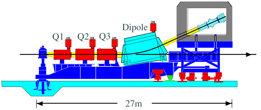
Figure 2.14: Side view of the HMS.

The magnets are cooled with 4K Liquid Helium provided by the CEBAF End Station Refrigerator (ESR). Under standard operating conditions, the HMS magnets require a flow of approximately 4 grams/second, running in parallel to the four magnets, to keep the magnet reservoir full and provide cooling for the current leads. The quadrupoles are cold Iron superconducting magnets. Soft Iron around the superconducting coil enhances the central field and reduces stray fields. Table 2.5 shows the size and operating parameters of the HMS quadrupoles. The quadrupoles are ‘degaussed’ by running the currents up to 120% of their 4 GeV/c values, and then lowering the currents to the desired values. The quadrupole current is provided by three Danfysik System 8000 power supplies. These supplies are water cooled and can provide up to 1250 Amps at 5 Volts. In addition to the quadrupole coils, each magnet has multipole windings. The correction coils are powered by three HP power supplies, capable of providing up to 100 Amps at 5 Volts. The multipole corrections to the quadrupoles were measured to be small when the magnet was mapped, and it was decided not to use the multipole correction coils for the standard point-to-point tune.

magnet	effective	inner pole	$I_{max}$*
	length	radius
Q1	1.89 m	25.0 cm	580 A
Q2	2.155 m	35.0 cm	440 A
Q3	2.186 m	35.0 cm	220 A
*$I_{max}$ is for 4.0 GeV/c central momentum.

Table 2.5: Operating parameters of the HMS quadrupoles.

The HMS dipole is a superconducting magnet with a $25^{\circ}$ bending angle for the central ray. The dipole has a bend radius of 12.06 m and a gap width of 42 cm. Its effective field length is 5.26 m (calculated assuming a perfect dipole, with a 25^∘ bend and 12.06 m radius). It has been operated at up to 1350 Amps, corresponding to a central momentum of just over 4.4 GeV/c. The current is provided by a Danfysik System 8000 power supply capable of providing up to 3000 Amps at 10 Volts.

The HMS was operated in its standard tune: point-to-point in both the dispersive and non-dispersive direction. This tune provides a large momentum acceptance, solid angle, and extended target acceptance (see table 2.6). In this tune, Q1 and Q3 focus in the dispersive direction and Q2 focuses in the transverse direction. The optical axis of each quadrupole was determined using the Cotton-Mouton method [50]. The optical axes were found to be different from the mechanical axes by up to 2mm, and all magnets were aligned with respect to the optical axis. When installed, the magnets were aligned to 0.2 mm, but move slightly when the spectrometer is rotated. The magnets move up to 1.0 mm, but the positions are reproducible up to 0.5 mm. The dipole field is monitored and regulated with an NMR probe. The quadrupole fields are regulated by monitoring the current in the magnets. The fields of dipole and quadrupoles are stable at the $10^{-4}$ level. Table 2.6 summarizes the design goals from the CEBAF Conceptual Design Report [51] and final performance of the HMS.

	CDR	Final Design
Maximum central momentum	6.0 GeV/c	7.4 GeV/c*
Momentum bite[($p_{max}-p_{min})/p_{0}$]	$20\%$	$20\%$
Momentum resolution [$\delta p/p$]	$0.1\%$	$0.02\%$ (0.04%)
Solid angle (no collimator)	10 msr	8.1 msr
Angular acceptance - scattering angle		$\sim\pm 32mr$
Angular acceptance - out-of-plane		$\sim\pm 85mr$
Scattering angle reconstruction	0.1 mr	0.5 mr (0.8 mr)
Out-of-plane angle reconstruction	1.0 mr	0.8 mr (1.0 mr)
Extended target acceptance	20 cm	$\sim 10$ cm
Vertex reconstruction accuracy	$\sim 1$ mm	2 mm (3 mm)
* So far, the HMS has only been operated at settings below 4.4 GeV/c.

Table 2.6: HMS design goals and final performance. Values in parenthesis include the effects of a 200$\mu$m resolution per plane in the drift chambers, and multiple scattering for a 2.5 GeV/c electron.

The initial model used to determine the field settings was generated using the COSY INFINITY program from MSU [52]. The quadrupoles were all field mapped, and the maps were used to determine the conversion between current and field integral ($\int B\cdot dl$). When the first optics test runs were completed, the final field values were fine tuned from the model values in order to give the best focus at the focal plane. The focal plane is defined as the surface created by varying the angles of the initial rays, and determining the point where they are focussed by the magnetic system. We use an approximation that this surface is a plane, whose position and angle are defined by the behavior of this surface near the focal point for rays at the central momentum. This is what we refer to as the ‘true’ focal plane. The focal plane we use when analyzing the data is defined to be the plane perpendicular to the central trajectory, at the position where the central ray intersects the true focal plane. In the HMS, the focal plane is located near the center of the the two drift chambers. The true focal plane of the spectrometer is actually tilted $\sim 85^{\circ}$ from the ‘detector’ focal plane. The focal plane coordinate system is designed to follow the TRANSPORT [53] convention. $x_{fp}$ is the position in the dispersive direction ($\hat{x}$ points downwards for vertical bend spectrometers), $y_{fp}$ is the position in the non-dispersive direction ($\hat{y}$ points left when looking at the spectrometer from the target). The $\hat{z}$ direction is parallel to the central ray (such that $\hat{x}\times\hat{y}=\hat{z}$) with $z=0$ at the focal plane. $x^{\prime}_{fp}$ and $y^{\prime}_{fp}$ are the slopes of the rays at the focal plane ($\frac{dx_{fp}}{dz}$ and $\frac{dy_{fp}}{dz}$). When the tracks are reconstructed to determine the location and direction of the events at the target, the same coordinate system is used. $x_{tar}$ is the vertical position ($\hat{x}$ points downwards), $y_{tar}$ is the horizontal position perpendicular to the spectrometer angle ($\hat{y}$ points left when looking at the spectrometer from the target), and $z_{tar}$ is the horizontal position in the direction perpendicular to $y_{tar}$ ($\hat{x}\times\hat{y}=\hat{z}$). $x^{\prime}_{tar}$ and $y^{\prime}_{tar}$ are the slopes of the ray at the target ($\frac{dx_{tar}}{dz}$ and $\frac{dy_{tar}}{dz}$). While $x^{\prime}$ and $y^{\prime}$ are slopes, they are nearly equal to the out-of-plane and in-plane angles for events in the spectrometer acceptance. Therefore, they are often referred to as the angle relative to the spectrometer angle and given in units of radians or mr. However, they are in fact the tangents of those angles, and are treated as such when calculating kinematics.

The magnet currents were initially set according to the values expected from the model of the spectrometer and the nominal current to field conversion. The quadrupole fields were then varied in order to determine the derivatives $\frac{dx_{fp}}{dQ_{i}}$ and $\frac{dy_{fp}}{dQ_{i}}$, where $x_{fp}$ and $y_{fp}$ are the $x$ and $y$ positions of the focal point for $\delta=0$, and $Q_{1,2,3}$ correspond to the settings of the three quadrupoles. Once these derivatives were measured, Q2 was adjusted in order to center the $y$ (horizontal) position of the focal point, and Q1 was adjusted to center the focal point in $x$. This procedure was iterated once more to give the best focus at the focal point. The focus is relatively insensitive to the Q3 value, so Q3 was fixed during the Q1 and Q2 adjustments. The ratio of Q1 to Q2 after making these adjustments was consistent with the COSY Monte Carlo (described in section 3.3.8), so Q3 was set so that the ratio of Q3 to Q1 matched the COSY model. From analyzing (e,e’p) data at multiple energies, it was found that the dipole field was 0.9% below the desired value, and the dipole field was readjusted. Figure 2.15 compares the focal plane distribution of events and reconstruction of events at the collimator for the final tune and for the COSY model, taken with an octagonal collimator in place. The model uses a uniform cross section in momentum and scattering angle. The data is taken at p=3.21 GeV, $\theta=15^{\circ}$, and the cross section is roughly uniform in momentum, but decreases with increasing scattering angle (decreasing $y^{\prime}_{tar}$, labeled as hsyptar in the figure).

Figure 2.15: HMS focal plane distributions (left) and reconstructed distributions at the collimator (right). The top distributions are from data and the bottom are from the HMS Monte Carlo model with uniform illumination. The left plots show $x$ versus $y$ at the focal plane. The right plots show $x_{tar}$ versus $y_{tar}$ projected to the collimator (126.2 cm from the target).

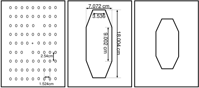
Figure 2.16: The HMS large and small collimators and sieve slit. The small collimator was not used during the experiment. Two holes are missing in order to verify proper left-right and top-bottom reconstruction. The central hole is smaller than the others in order to measure the angular resolution of the reconstructed data.

A slit system was installed in front of the first quadrupole, allowing remote insertion of various collimators. There are three HEAVYMET (machinable Tungsten with 10% CuNi; density=17 g/cm³) collimators and one blank space in the slit box. The three collimators are shown in figure 2.16. The first collimator is a 3.175 cm thick sieve slit used for optics testing. It is an array of small holes (0.508 cm diameter) used to compare focal plane distributions to data with known angular distributions in order to study the optics of the spectrometer. Two holes are missing in the sieve slit in order to verify proper left-right and top-bottom reconstruction. The central hole is smaller than the others in order to measure the resolution of the angular reconstruction. Figure 2.17 shows the event reconstruction at the front of the sieve slit. The other two collimators are octagonal apertures designed to limit the solid angle acceptance of the HMS. Both are 6.35 cm thick and have flared holes that match the acceptance of the spectrometer. The large slit has a solid angle of $\sim 6.8$ msr and was designed to keep losses within the spectrometer low for a point target (no loss in the magnetic elements for a $\pm$5% momentum bite, $<$2% for a momentum bite of $\pm 10$%). The small slit was designed to give small losses in the spectrometer for an extended target ($\mathrel{\raise 1.29167pt\hbox{$<$}\mkern-14.0mu\lower 2.58334pt\hbox{$\sim$}}$0.1% for $\pm$10% with a 4 cm target, $\mathrel{\raise 1.29167pt\hbox{$<$}\mkern-14.0mu\lower 2.58334pt\hbox{$\sim$}}$0.1% for $\pm$5% with a 10cm target). For e89-008, all data was taken using the large octagonal collimator.

Figure 2.17: HMS reconstruction at the Sieve Slit. The vertical hole spacing corresponds to 19.90 mr steps, and the horizontal spacing corresponds to 11.93 mr steps. Note that two holes are missing in order to verify the sign of the angle reconstruction. The central hole is smaller than the others in order to measure the angular reconstruction resolution.

2.5.2 Short Orbit Spectrometer

The SOS was primarily intended to detect hadrons in coincidence with the HMS. Its central trajectory from the target to the back of the detector stack is short ($\sim$9 m) in order to allow detection of short lived particles (Kaons and low momentum pions). It has large solid angle ($\sim$9 msr) and very large momentum bite ($\pm 20\%$), but a somewhat limited extended target acceptance ($\sim$2-3 cm).

The SOS was made based on a $QD\overline{D}$ design developed for the MRS (medium resolution spectrometer) at LAMPF. It consists of a quadrupole (QS) which focuses in the horizontal (non-dispersive) direction followed by two dipoles (BM01 and BM02) which bend the beam up $33^{\circ}$ and then down $15^{\circ}$. Figure 2.18 shows a side view of the SOS magnets. All three magnets and the detector hut rest on a common carriage assembly, and the dipoles share a common yoke. The carriage can be elevated in the rear by hydraulic jacks, allowing the SOS to go out of plane by up to $20^{\circ}$. These jacks can also be used to level the spectrometer for in-plane measurements as the spectrometer rests $0.15^{\circ}$ below the horizontal without the jacks. During the experiment, the jacks were not used. However, for inclusive measurements, there is no need to correct for an offset in the out-of-plane angle.

Figure 2.18: Schematic side view of the SOS magnets.

The quadrupole and dipoles are water cooled non-superconducting magnets. They are powered by three separate InverPower power supplies which can be remotely controlled from the counting house. The power supplies can reverse the output polarity, allowing running for positive and negative particles. The QS and BM02 supplies provide 1000 Amps at 160 Volts and the BM01 supply provides 1000 Amps at 250 Volts. The maximum momentum attainable is limited by the current that can be provided to BM01. However, at the maximum central momentum setting (1.75 GeV), QS is driven to $\sim$170 Volts (which is within the over drive capacity of the supply) and the magnets are near saturation, so while an increase in the maximum momentum would be possible, any increase would have a significant effect on the optics. The magnets and power supplies are cooled by the Hall C Low Conductivity Water system which provides water at 250 PSI. For the SOS, the optical axis of each magnet was found to be the same as its mechanical axis within 0.1mm, and so the magnets were positioned using the mechanical axes. When installed, the magnets were aligned to 0.2 mm, but can shift when the spectrometer is rotated. The magnets move radially up to 2 mm, but the positions are reproducible to better than 0.5 mm. The movement of the magnets is the main contribution to the uncertainty in the spectrometer angle. The dipole and quadrupole magnets have Hall probes which measure the fields and are used to regulate the magnet settings. There is a non-linearity in the field versus current at high momenta. At high SOS momenta ($\mathrel{\raise 1.29167pt\hbox{$>$}\mkern-14.0mu\lower 2.58334pt\hbox{$\sim$}}$1.6 GeV/c), the true momentum for the spectrometer is slightly lower than that expected from the current settings ($\sim$0.6% at 1.75 GeV/c). See section 2.5.3 for more details. However, the SOS data was all taken at momentum values below 1.5 GeV/c, except for some detector calibration runs. The standard degaussing procedure for the SOS involves setting the polarity of the magnets to the desired polarity, increasing the currents to their maximum values, then reducing the currents to zero and switching to the opposite polarity. The currents are again raised to their maximum values and then reduced to zero, and the polarity is set back to the desired value. The quadrupoles can then be raised to the desired currents. As long as the currents are increased, the magnets will stay on the correct side of the hysteresis curve and degaussing is unnecessary. If the current is lowered, or the polarity reversed, the degaussing procedure is repeated before the magnets are set to their desired values.

The SOS optics have been studied in two standard tunes. For this experiment the SOS was operated in the point-to-point tune, with point-to-point focusing in both the dispersive and non-dispersive directions. This tune has a large solid angle and very large momentum bite, but a small extended target acceptance (see table 2.7). The ratio of the dipole fields ($D/\overline{D}$) was determined by integrating the field for the central trajectory using field maps made of the dipoles. Because QS was never mapped, the quadrupole field settings were determined using COSY optics models, generated assuming that QS was a perfect quadrupole. These settings were tested by comparing the model to elastic scattering data taken with a sieve-slit. The analysis of the optics data showed that the quadrupole field was higher than expected for the current, and the quadrupole current was lowered 7% in order to give the field used in the model. Figure 2.19 shows the reconstruction of events at the front face of the sieve slits. As is clearly seen, the out-of-plane angle reconstruction is much better than the scattering angle reconstruction. Figure 2.20 compares the distribution at the ‘detector’ focal plane and at the collimator for data and Monte Carlo. The Monte Carlo was run with a uniform cross section in $\delta$ and $\theta$, while the data has a small $\delta$ and $\theta$ dependence in the cross section. The comparison at the focal plane shows some small differences, but since we fit reconstruction matrix elements to calibration data for the SOS (section 3.3.8), the reconstructed physics quantities are not affected by this difference.

The focal plane we use is defined to be perpendicular to the central ray, and located 6 cm in front of the first drift chamber. The true focal plane of the spectrometer is tilted forward from the ‘detector’ focal plane (used in the software) by $\sim 70^{\circ}$. Table 2.7 summarizes the design goals and true performance of the SOS.

Figure 2.19: SOS reconstruction at the Sieve Slit. The vertical hole spacing corresponds to 20.11 mr steps, and the horizontal spacing corresponds to 12.07 mr steps, except for the central three columns, which are spaced by 8.04 mr. The three columns in the center are not cleanly resolved in the plot. Note that two holes are missing in order to verify the sign of the angle reconstruction and that the central hole is smaller than the others.

Figure 2.20: SOS focal plane distributions. The top distributions are from data and the bottom from the SOS Monte Carlo. The left plots show $x$ versus $y$ at the focal plane. The right plots show $x_{tar}$ versus $y_{tar}$ projected to the collimator (126.2 cm from the target).

	CDR	Final Design
Maximum central momentum	1.5 GeV/c	1.75 GeV/c
Momentum bite[($p_{max}-p_{min})/p_{0}$]	$40\%$	$40\%$
Momentum resolution [$\delta p/p$]		$0.1\%$
Solid angle (no collimator)	9 msr	10.7 msr
Angular acceptance - scattering angle	$\pm 60$ mr	$\pm 70$ mr
Angular acceptance - out-of-plane	$\pm 40$ mr	$\pm 40$ mr
Scattering angle reconstruction		4.0 mr
Out-of-plane angle reconstruction		0.5 mr
Extended target acceptance		$2-3$ cm
Vertex reconstruction accuracy		1.2 mm

Table 2.7: SOS design goals and final performance. Resolutions include effects of a 200$\mu$m resolution per plane in the drift chambers.

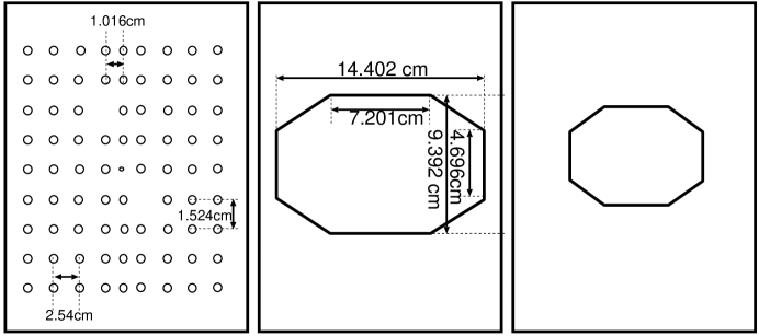
Figure 2.21: The SOS large and small collimators and sieve slit. The small collimator was not used during the experiment. The central three columns of the sieve slit are closer together than the other columns. Two holes are missing in order to verify proper left-right and top-bottom reconstruction. The central hole is smaller than the others in order to measure the angular resolution of the reconstructed data.

A slit system, nearly identical to the HMS slit system, was installed in front of the SOS quadrupole, allowing remote insertion of various collimators. There are three HEAVYMET collimators and one blank space in the slit box. The three collimators are shown in figure 2.21. The first collimator is 3.175 cm thick and has an array of small holes (0.508 cm diameter) used to study the optics of the spectrometer. The holes have a 1.524 cm vertical spacing and a 2.54 cm horizontal spacing, except for the central three columns which have a 1.016 cm spacing. Two holes are missing so that proper left-right and top-bottom reconstruction can be verified. The central hole is smaller so that the resolution of the angular reconstruction can be measured. The other two collimators are octagonal apertures designed to limit the solid angle acceptance of the SOS. Both are 6.35 cm thick and have flared holes that match the acceptance of the spectrometer. The large collimator has a solid angle of $\sim$7.55 msr and was designed to eliminate losses within the spectrometer for a point target (no loss for a momentum bite of $\pm 10$ %) and to keep losses at $\sim$1% for a 2 cm target. The small collimator was designed to keep losses small ($<1\%$) for a 2cm target using a $\pm 20\%$ momentum bite. All of our data was taken using the large octagonal collimator. Figure 2.22 shows the acceptance for an extended target with the large collimator. The geometry of the collimators for both the HMS and SOS is described in table 2.8

Slit	d$\Omega$	Central	Central	Shape
	(msr)	Width	Height
large HMS	6.74	$\pm$27.5mr	$\pm$70.0mr	Octagonal, Flared
small HMS	3.50	$\pm$20.0mr	$\pm$50.0mr	Octagonal, Flared
large SOS	7.55	$\pm$57.5mr	$\pm$37.5mr	Octagonal, Flared
small SOS	3.98	$\pm$32.5mr	$\pm$35.0mr	Octagonal, Flared

Table 2.8: Size of the HMS and SOS collimators.

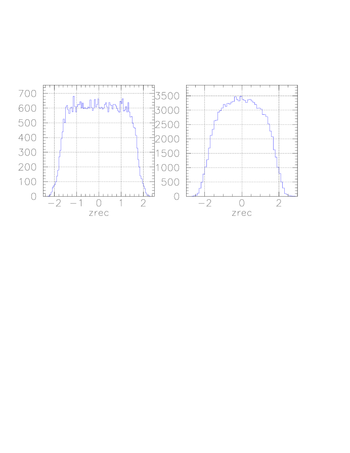
Figure 2.22: SOS extended target acceptance from the SOS Monte Carlo. The figure on the left is the distribution of accepted events versus position along the beam with a $\pm$5% $\delta$ cut applied. The right figure is for the $\delta$ cut used in the analysis, $16\%<\delta<12\%$.

2.5.3 Spectrometer Momentum Calibration

If the beam energy is known, the spectrometer momentum can be determined by measuring elastic H(e,e’) scattering. The uncertainties in this method come from the uncertainty in the beam energy, and the uncertainty in the spectrometer angle. The main uncertainty comes from the beam energy, and limits the spectrometer momentum calibration to $\sim$0.2%.

The spectrometer momentum was also determined by taking a series of elastic scans at different angles, all with the same beam energy. Even if the beam energy is only known at the 0.2% level, the variation of reconstructed $W^{2}$ is sensitive to the uncertainty in the spectrometer momentum. For the HMS, the difference between the measured momentum and the expected momentum had a small $p$-dependence. The fractional momentum variation was $\sim$ 3x10^-4 over the range of angles measured. Figure 2.23 shows the value of $W^{2}-M^{2}$ for the elastic peak as a function of $p_{HMS}$. The curve is a two-parameter fit to the data assuming a fixed offset in $\Delta p_{HMS}/p_{HMS}$ and $\Delta E/E$. The fit gives a -0.15% shift to the assumed beam energy of 4045 MeV (for a beam energy of 4038.9 MeV), and a momentum offset consistent with zero. The uncertainties from the fit are $\delta E/E$=0.04%, $\delta p/p$=0.03%. This energy is compared to the Hall C Arc measurement taken at the same time (4036.1$\pm$0.6 MeV), and used to verify the Arc energy measurements. The energy used in the analysis of the e89-008 data (4045 MeV) was based on the Arc measurement taken during the run.

Figure 2.23: HMS Momentum Calibration from Elastic Scan at Fixed Beam Energy. The points are $W^{2}-M^{2}$ for the elastic peak as a function of $p_{HMS}$. The curve is a two-parameter fit to the data assuming a fixed offset in $\Delta p_{HMS}/p_{HMS}$ and $\Delta E/E$.

The SOS showed variations of $<$0.2% for momentum below 1.5 GeV/c, but decreased at higher momenta, due to a non-linearity of the magnet at fields near the maximum (1.75 GeV/c). At 1.7 GeV/c, the momentum is $\sim$0.6% low. For our data, the SOS momentum is always below 1.5 GeV/c. Previous experiments, using hydrogen elastic to check the SOS momentum at a variety of angles and momentum settings show typical offsets of $\sim$0.1% for momenta below 1.5 GeV/c. We therefore assign an uncertainty of 0.1% to the SOS momentum.

2.5.4 Spectrometer Angle Calibration

The angle of the spectrometer is measured by comparing the position of the back of the spectrometer to marks that have been scribed on the floor of the Hall. This comparison is good to better than 2 mm, and gives an angular uncertainty of less than 0.1 mr in the HMS, and less than 0.3 mr in the SOS. However, the main uncertainty in the spectrometer angle comes from the motion of the magnets as the spectrometer is rotated. For HMS angles below 70^∘, the magnets are stable to approximately 1 mm. The first magnet is approximately 1.5m from the pivot, giving an uncertainty of $\mathrel{\raise 1.29167pt\hbox{$<$}\mkern-14.0mu\lower 2.58334pt\hbox{$\sim$}}$1.0 mr in the HMS angle. For the SOS, the position variation can be up to 2 mm, giving an uncertainty of $\mathrel{\raise 1.29167pt\hbox{$<$}\mkern-14.0mu\lower 2.58334pt\hbox{$\sim$}}$1.5 mr. Because the magnet positions are reproducible at the $\sim$0.5 mm level, this uncertainty could be reduced by carefully surveying the magnet positions at each spectrometer angle. However, the uncertainty in the scattering angle introduces a small uncertainty in the cross section compared to uncertainties in the beam energy and momentum.

Measurements of elastic H(e,e’p) scattering was measured at a variety of kinematics and was used to check for momentum and angle offsets in the spectrometers. The offsets determined this way depend on the assumed beam energy, and it is not always possible to distinguish HMS offsets from SOS offsets. However, the momentum offsets were $\mathrel{\raise 1.29167pt\hbox{$<$}\mkern-14.0mu\lower 2.58334pt\hbox{$\sim$}}0.03\%$ for the HMS, and $\mathrel{\raise 1.29167pt\hbox{$<$}\mkern-14.0mu\lower 2.58334pt\hbox{$\sim$}}0.1\%$ for the SOS (except at large momenta, $\mathrel{\raise 1.29167pt\hbox{$>$}\mkern-14.0mu\lower 2.58334pt\hbox{$\sim$}}$1.6 GeV/c). The HMS and SOS angular offsets vary at the $\pm 1.0$ mr level, which are consistent with the limits from the magnet motion. For the HMS, the inclusive elastic scan can also be used to look for angular offsets. If one assumes that the momentum is well known, then the elastic scan sets a limit of $\sim$0.4 mr to the uncertainty in the scattering angle. For determining errors in the cross section due to spectrometer angle offsets, we assume an RMS uncertainty of 0.5 mr for the HMS, and $\pm 1.5$ mr for the SOS.

2.6 Detector Package

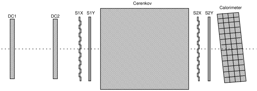
Figure 2.24: Schematic diagram of the HMS detector hut.

The standard HMS and SOS detector packages are very similar. Each spectrometer contains two drift chambers, two sets of x-y hodoscopes, a gas Čerenkov detector, and a lead glass shower counter. The drift chambers provide tracking information, the hodoscopes are used to form the primary trigger, and the calorimeter and Čerenkov signals are used for particle identification (pion rejection) in the trigger and in the offline analysis. A schematic of the HMS detector package is shown in figure 2.24. The layout of the SOS detector package (figure 2.25) is more compact, but is otherwise nearly identical except that the Y planes of hodoscopes come before the X planes, and there is an aerogel Čerenkov behind the gas Čerenkov (not shown in figure 2.25). The aerogel Čerenkov was not utilized for this experiment.

The high voltage for all of the detectors is provided by CAEN high voltage power supplies. Table 2.9 describes the three types of High voltage cards used in the detector huts. The HMS and SOS CAEN crates are located inside the detector huts in order to shield them from the high radiation environment that exists when beam is in the hall. The communication ports in the crates in each hut are daisy chained together and can be monitored and controlled from the counting house by either a terminal RS232 connection, or through the EPICS (Experimental & Physics Industrial Control System [54]) slow control system. The EPICS system controls the crate through a VME CAEN-net controller card located in the huts. The power supplies can be controlled from the counting house through a Tcl/Tk X-windows interface.

HV Card	$V_{max}$	$I_{max}$	Detectors
A403/A503	-3000 V	3.0 mA	Hodoscope/Calorimeter
A503P	+3000 V	3.0 mA	Čerenkov
A505	-3000 V	200 $\mu$A	Drift Chambers

Table 2.9: CAEN HV cards used in HMS and SOS.

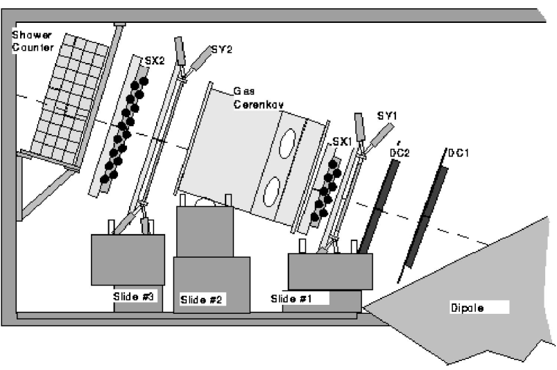
Figure 2.25: diagram of the SOS detector hut.

2.6.1 Detector Supports

The SOS detector package was designed to be very compact in order to allow detection of short lived particles. Therefore, the elements are mounted as closely together as possible. All of the detectors except the calorimeter are mounted on supports which allow the detectors to be pulled out of the hut without removing them from their supports and without disconnecting the power and readout cables. This makes it possible to work on the detectors without disassembling the support structure and allows the detectors to be mounted very closely to one another. There are four separate supports for the detectors. The first three are sliding mounts and the last is a fixed support. The first sliding mount supports the two drift chambers (DC1 and DC2) and the first pair of hodoscope planes (S1X and S1Y), the second supports the gas Čerenkov detector, and the third holds the rear hodoscope planes (S2Y and S2X) and the aerogel Čerenkov detector. The lead glass calorimeter is supported by a fixed frame, mounted to the ceiling and rear wall of the detector hut. A side view of the detectors and support system is shown in figure 2.25.

The drift chamber positions have been measured by the CEBAF survey group with respect to fixed survey marks on the SOS dipole. The drift chamber position are known to 0.4 mm and the differences between the measured drift chamber positions and their desired positions is corrected for in the tracking software. The other detector positions are known to within a few mm from measurements in the huts and surveys of the detector stands. Since the position of the drift chambers was well known, we used data from electron scattering to determine the positions of the other detectors with respect to the chambers. The sliding mounts have a position reproducibility of better than 0.25mm, and are not a leading cause of position uncertainty.

The HMS hut is much larger, and so it was not necessary to mount the detectors as close together. The detectors are mounted on frames that connect to the carriage that supports the magnets. This insures that the detectors stay at a fixed position with respect to the magnets. The shielding hut is on a separate support. The final detector positions used in the analysis were determined following the same procedure as in the SOS.

2.6.2 Drift Chambers

The HMS drift chambers consists of six planes, two measuring $x$ (the dispersive direction), two measuring $y$ (the non-dispersive direction), and two that were rotated $\pm 15^{\circ}$ from the $x$ planes (the $u$ and $v$ planes). The planes were ordered $x,y,u,v,y^{\prime},x^{\prime}$ as seen by incoming particles. The chambers had an active area of approximately 113 cm ($x$) by 52 cm ($y$) with a sense wire spacing of 1 cm. Figure 2.26 shows a front view of the HMS chambers. The planes were spaced 1.8 cm apart and the two drift chambers were separated by 81.2 cm. Each active plane contained alternating field and sense wires. The sense wires (anodes) are 25 $\mu$m diameter Gold-plated tungsten wire, and the field wires (cathodes) are 150 $\mu$m Gold-plated copper-beryllium wires. In between these planes were planes of guard wires. The sense wires detect the ionization from passing charge particles, and the field and guard wires are maintained at negative high voltage in order to isolate the sense wires and provide the electric field that attracts the ionized electrons to the sense wires. The voltage for the guard wires varied depending on its distance from the nearest sense wire, from -1800 V to -2500 V. This provided equipotential contours that were roughly circular. Figure 2.27 shows a cross section of the $y$ and $y^{\prime}$ planes. The distance between the wire and the track is determined by the drift time of the electrons.

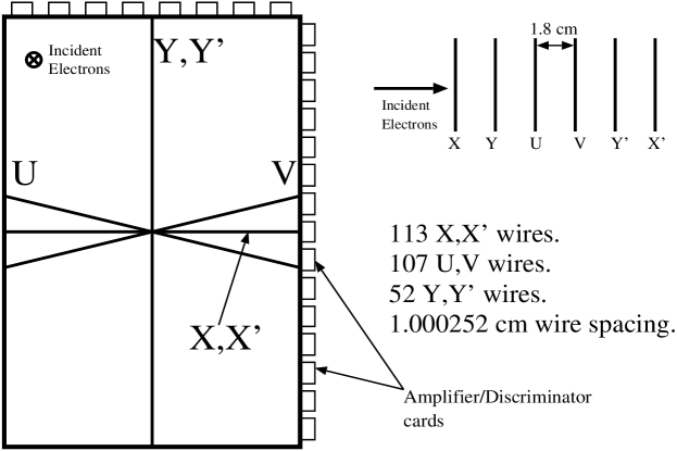
Figure 2.26: Front view of the HMS drift chambers. The lines shown within the chamber indicate the region of coverage for the $x$, $y$, and $v$ wire planes. The position of the readout cards is shown on the outside of the chamber.

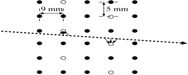
Figure 2.27: HMS drift chamber cell structure for the $y$ and $y^{\prime}$ planes. The black wires are guard wires, and the white wires are the sense wires. As the charged particle ionizes the gas in the drift chambers, the electrons are attracted to the sense wire by the electric potential generated by the field wires. The wires in the chamber are smaller than shown here.

When a charged particle passes through the chamber, the gas is ionized, and the liberated electrons are attracted to the nearest sense wire by the voltage differential maintained by the chamber. By detecting which wire sensed the particle, the position is measured with a 0.5 cm accuracy (half the wire spacing). The time required for the electrons to drift to the wire is measured by taking the time difference between the passage of the charged particle and the signal on the wire. This allows a much better determination of the position of the particle. By measuring the position with 6 planes, the $x$ and $y$ position of the particle and it’s trajectory through the chamber can be measured. A complete description of the HMS drift chambers can be found in [55].

The HMS chambers are filled with an argon/ethane mixture (equal amounts by weight) along with $\sim$1% Isopropyl alcohol. The gas mixing system is located in a shed above the experimental hall and provides parallel gas streams to the two chambers. An MKS 647 menu driven 4-channel controller operates the system. The gas flow is controlled with MKS 1259c proportional mass flow control valves. The flow is monitored by temperature controlled alcohol bubblers on the gas lines going to the chambers.

The sense wires are read out in groups of 16, each connected to a LeCroy 2735DC or Nanometric N-277-L amplifier/discriminator card. The discriminator thresholds for all of the cards is provided by single external Acopian low voltage supply which was controlled remotely from the counting house. The threshold voltage supply in the counting house was set between 5.0 and 5.5 Volts during the experiment, but there is a 1-2 Volt drop between the source and the chambers downstairs. The signals from the discriminator cards are carried on twisted pair ribbon cable and go to LeCroy 1877 multi-hit Time-to-Digital Converters (TDCs) located in the back of the detector hut. The trigger is formed in the counting house and a TDC stop signal is sent back to the hall. The TDCs can store all hits (up to 16 per wire) that came within the last 32 $\mu$s. Because the total time between a particle in the spectrometer and the trigger arriving at the TDC is less than 2 $\mu$s, we programmed the TDCs to read out events within a window of $\sim$4$\mu$s. The drift chamber TDCs measure the time that the wire detected the electrons created by the ionization of the chamber gas, relative to the time of the trigger.

Using the hodoscope TDCs to determine the time that the particle passed through the focal plane (again, relative to the trigger), we can determine the time it took for the electrons created by the ionizing particle to ‘drift’ to the wire. This drift time is converted into a drift distance which is then added to the wire position in order to get the position of the event. The conversion from drift time to drift distance is determined by comparing the distribution of drift times in the chamber with expected position distributions of events within a cell. Combining the hits in all six planes allows us to determine on which side of each wire the particle passed. We make a small angle approximation and assume that for planes that measure the same coordinate, but which are offset by 1/2 cell, the particle passed between the two wires that fired. For events where only one of the two matching planes fired and for unmatched planes ($u$ and $v$), we look through all left-right combinations and take the track with the minimum $\chi^{2}$. The final position resolution is approximately 280 $\mu$m per plane.

Two types of drift chambers were built for the SOS at Brookhaven National Laboratory. The SOS was designed to hold two Type I chambers (DC1 and DC2), in the front of the detector package and one Type II chamber (DC3) at the rear. The Type I and Type II chambers are nearly identical, but the Type II chambers were larger in order to contain the entire beam envelope near the back of the detector package. During e89-008 running, only the two Type I chambers were installed. Each chamber is constructed of sixteen layers of 0.3175 cm G10 frames, sandwiched between two 1.27 cm Al frames. The G10 frames support alternating planes of wires and cathode foils, as shown in figure 2.28. The wire planes consist of alternating sense and field wires. The sense wires (30 $\mu$m diameter) are separated by 1 cm within the plane and detect the electrons released as the particle ionizes of the gas in the chamber. The field wires (60$\mu$m diameter) alternate with the sense wires. The field wires and cathode foils are maintained at a large negative high voltage (-1975 V) in order to provide the field for the sense wires. The wire planes come in pairs that measure positions in the same direction and have their wires offset by 0.5 cm. The wire positions were measured during chamber construction and matched the expected values within the uncertainty of the measurement ($\pm 87\mu$m). The $x$ and $x^{\prime}$ planes measure the position in the dispersive direction, the $u/u^{\prime}$ planes are rotated $60^{\circ}$ clockwise from the $x$ plane, and the $v/v^{\prime}$ planes are rotated $60^{\circ}$ counterclockwise from $x$. There are 64 wires in the $x$ and $x^{\prime}$ planes and 48 wires in the $u,u^{\prime},v,$ and $v^{\prime}$ planes. The active area of the chambers is 63 cm by 40 cm, with cutoffs in the corners as shown in figure 2.29.

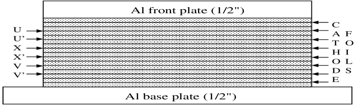
Figure 2.28: Cross section of the SOS drift chambers.

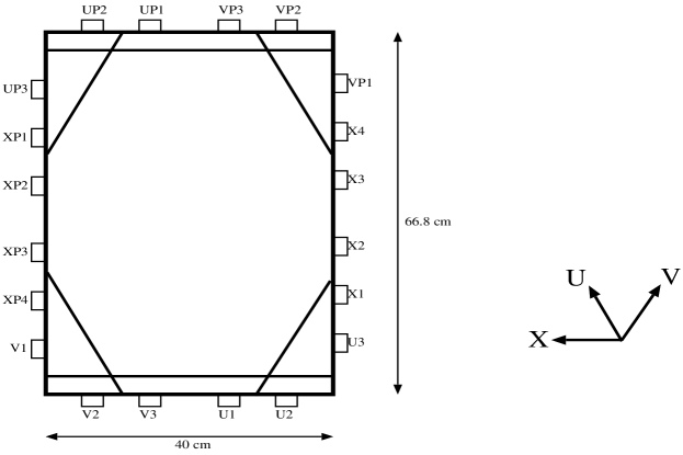
Figure 2.29: Front view of the SOS drift chambers. The position of the readout cards is shown on the outside of the chamber.

The SOS used the same gas mixture and gas handling system as the HMS and nearly identical readout electronics. The threshold voltage for the SOS was set at 1.5 V. The drift distances and left-right determinations were made in the same way as in the HMS. However, because all of the SOS planes come in pairs, the small angle approximation can be used to make the left-right determination for any pair of matched planes in which both planes are hit. An event which fires all six planes in a chamber has its left-right pattern determined unambiguously. The final position resolution for the SOS drift chambers is approximately 180 $\mu$m per plane.

2.6.3 Hodoscopes

The HMS and SOS each have two pairs of (x-y) hodoscopes, identical except for size of the elements. Each hodoscope plane is constructed of 9 to 16 elements. The hodoscope elements are long narrow strips of BC404 scintillator with UVT lucite light guides and Philips XP2282B phototubes on both ends. When charged particles pass through the paddles, they ionize the atoms in the material. The liberated electrons excite molecular levels in the scintillator, which emit light when they decay. The light is detected by Photomultiplier Tubes (PMTs) at the ends of the paddles. The light emitted along the length of the paddles will be detected by PMTs after the light has had time to traverse the length of the paddle. Light that is not emitted along the length of the paddle, but which hits the surface of the scintillator at greater than the critical angle, will be completely reflected and will also reach the PMTs. The HMS scintillators are wrapped with one layer of aluminum foil and two layers of Tedlar to make them light tight with a minimum amount of additional material. The SOS scintillators are wrapped with 1 layer of Aluminized mylar and 1 layer of Tedlar. The scintillators have approximately 0.5 cm of overlap between the paddles in order to avoid gaps between the elements. In the HMS, all of the scintillators are 1.0 cm thick and 8 cm wide. The x elements are 75.5 cm long, and the y elements are 120.5 cm long. The x planes have 16 elements each and the y planes have 10 elements each, giving each x-y pair an active area of 120.5 cm by 75.5 cm. The front and back planes are separated by approximately 220 cm. In the SOS, the front hodoscope pair is smaller than the back. The front x plane (S1X) has 9 elements, 36.5 cm x 7.5 cm x 1.0 cm and the front y plane (S1Y) has 9 elements that are 63.5 cm x 4.5 cm x 1.0 cm. The total active area of the front hodoscope is 63.5 cm x 36.5 cm. The rear hodoscope planes are larger versions of the front planes. The S2X plane is made up of 16 elements, each 36.5 cm x 7.5 cm x 1.0 cm and S2Y has 9 elements, 112.5 cm x 4.5 cm x 1.0 cm. Once again, the widths and lengths of the planes were matched so that the full area (112.5 cm x 36.5 cm) is active. The front and back planes in the SOS are separated by approximately 180 cm.

Each scintillator element is read out by PMTs at both ends. The 8-stage PMTs are connected to bases with zener stabilization in the first and last two stages. The anode output from the bases is sent to a patch panel in the detector hut through $\sim$30 feet of RG58 cable, and then goes upstairs to the counting house through $\sim$450 feet of RG8 cable. The signals are run through a splitter, giving two signals with 1/3 and 2/3 of the amplitude of the original input signal. The smaller signal is put through $\sim$400 ns of RG58 cable delay and then goes to the Analog-to-Digital Converters (ADCs) that measure the integral of the signal. The larger signal goes to PS7106 leading edge discriminators. One set of outputs from the discriminators goes to custom logic delay modules and then to Fastbus TDCs and VME scalers. The other set of outputs is sent to a LeCroy 4654 logic module. This module generates the OR of all tubes on one side of a given plane (e.g. S1X+). The outputs we use for the trigger logic are the AND of the sets of tubes on each side of a plane (e.g. S1X $\equiv$ [S1X+] & [S1X-]) as well as the OR of the front (and back) pairs of planes (e.g. S1 $\equiv$ [S1X] + [S1Y]). Figure 2.30 is a diagram of the hodoscope trigger and readout electronics.

Figure 2.30: Hodoscope electronics diagram. The numbers adjacent to each module indicate the number of channels used in the HMS/SOS.

The hodoscope PMTs were gain matched using a ⁶⁰Co gamma ray source at the center of each element. The tube voltages are set such that the Compton edge from the gamma rays gives a pulse height of 175 mV at the discriminator inputs in the electronics room. Timing calibrations of the scintillators was done using data taken during running. Corrections for the ‘time walk’ due to variations in pulse height and offsets between the individual elements are determined using an offline fitting procedure. The procedure used to determine the timing calibrations is described in detail in section 3.2.2. The final timing resolution achieved was $\sim$100 ps per plane for the HMS, and 80-100 ps per plane for the SOS. The increased timing resolution in the SOS is offset by the reduced lever arm for the time-of-flight measurement, due to the smaller separation of the hodoscope planes. This gives a measurement of the particle velocity, $\beta=v/c$, with an RMS resolution $\sigma_{\beta}$=0.018 at $\beta=1$ for both spectrometers. The resolution improves as $\beta$ decreases because the uncertainty in the time at the hodoscope planes is constant, but the flight time is larger. Therefore, the relative uncertainty is proportional to the inverse of the time of flight, which is proportional to $\beta$.

2.6.4 Gas Čerenkov Detectors

The SOS gas Čerenkov was designed and built at the University of Colorado. A complete description of the detector can be found in the CEBAF SOS Čerenkov Detector Handbook [56]. The detector works by detecting the Čerenkov radiation emitted by particles when they move through a medium at velocities greater than $c/n$, where $c$ is the speed of light in vacuum, and $n$ is the index of refraction of the material. Charged particles moving above the speed of light in the medium will emit light in a forward pointing cone with an opening angle, $\theta_{c}$ defined by:

$$\cos{\theta_{c}}=1/\beta n$$ (2.3)

where $\beta$ is the velocity of the particle relative to the speed of light ($\beta=v/c$). By choosing the index of refraction of the material properly, the threshold velocity ($=c/n$) can be made such that electrons at the spectrometer momentum will emit Čerenkov radiation, and pions will not. Mirrors are used to focus the light onto photomultiplier tubes, which measure the Čerenkov light. The medium must be a material that will allow the Čerenkov light to propagate without significant loss, and which does not generate significant light from scintillation. For separating pions from electrons in a momentum range of 1-4 GeV, the index of refraction must be very small ($10^{-4}\mathrel{\raise 1.29167pt\hbox{$<$}\mkern-14.0mu\lower 2.58334pt\hbox{$\sim$}}(n-1)\mathrel{\raise 1.29167pt\hbox{$<$}\mkern-14.0mu\lower 2.58334pt\hbox{$\sim$}}10^{-3}$). Therefore, a gas can be used as the Čerenkov medium, and the type of gas and operating pressure can be chosen in order to maximize the signal for electrons, while minimizing scintillation and keeping the pion Čerenkov threshold above the spectrometer momentum. The signal increases as the amount of material increases, and so the density is increased until the index of refraction is as large as possible while still maintaining a pion threshold above the spectrometer momentum. Pions can produce a Čerenkov signal, causing the pion to be misidentified as an electron, if the pion produces a knock-on electron of sufficient energy to emit Čerenkov light. In order to reduce the rate of knock-on electrons produced, the entrance window to the Čerenkov tank is made as thin as possible. Because the total thickness of material that could cause knock-on electrons is dominated by the window and detector material immediately in front of the Čerenkov detector, the density of the gas has a very small affect on the rate of $\delta$-ray production.

The SOS Čerenkov detector is a nearly rectangular aluminum box, 99 cm high, 73.7 cm wide, and 111 cm long. The detector was filled with 1 atmosphere of Freon-12 (CCl₂F₂). The index of refraction for Freon-12 is 1.00108, giving an electron threshold of 11 MeV and a pion threshold of 3 GeV (well above the SOS maximum momentum). The expected signal is $\sim$11 photoelectrons for a relativistic electron. The average signal measured in the detector is $\sim$12 photoelectrons for events at the center of the mirror. The light is reflected onto four Burle 8854 photomultiplier tubes by four spherical mirrors. Each phototube has a Winston cone (a reflective cone around the phototube front face) designed to increase the effective solid angle of the tube. The entrance window is rectangular, 27.94 cm high and 60.96 cm wide, with 30.48 cm radius half circles on the top and bottom. The exit window is a 22.86 cm by 60.96 cm rectangle with 33.02 cm radius half circles above and below. Both windows are make of 254 $\mu$m Lexan film covered with 50.8 $\mu$m Tedlar film. The front window has a total thickness of 39 mg/cm², which is small compared to the thickness of the scintillator material in front of the window and the thickness of the Freon gas (530 mg/cm²), and therefore does not significantly increase the number of energetic $\delta$-rays that are usually the dominant contribution to pion misidentification.

The Freon pressure is maintained by the SOS Čerenkov gas handling system. There is a relief valve that will open at 0.5 PSI overpressure, and a solenoid valve that will open to allow freon to flow into the tank at 0.2 PSI underpressure. The solenoid valve is controlled by an Omega pressure meter and the differential pressure is displayed on a monitor in the counting house. Typical pressure variations are at the 0.05 PSID level, corresponding to normal atmospheric pressure changes. The tank is filled by manually opening a release valve at the top of the tank and the freon input valve. The freon valve must be manually adjusted to maintain a pressure of about +0.07 PSID. Approximately 15 kg of Freon is allowed to flow into the tank. (several times the amount necessary to fill the tank). For perfect mixing, this would give a final gas purity of 95$\%$. Because Freon is denser than air and we fill from the bottom and exhaust through the top, the final purity is $>95\%$.

The HMS Čerenkov tank is cylindrical, with an inner diameter of $\sim$150 cm and a length of $\sim$165 cm. The effective length (before the mirrors) is approximately 120 cm. The tank is designed to run at gas pressures of up to 3 atmospheres, as well as running below atmospheric pressure. This allows the Čerenkov to be set up for e/$\pi$ separation using nitrogen at $\sim 1$ atmosphere of pressure, or $\pi$/p separation using 2-3 atmospheres of Freon-12. For this experiment, the tank was filled with 0.42 atmospheres of Perfluorobutane (C₄F₁₀, $n$=1.00143 at 1 atmosphere, 300K) giving an index of refraction of 1.0006. This gives a pion threshold of just over 4 GeV/c and electron threshold of $\sim$15 MeV/c). The expected yield was $\sim$11 photoelectrons, and the average measured signal from an electron was $\sim 10$ photoelectrons. There were two mirrors at the back of the tank which reflected and focussed the Čerenkov light into two 5-inch Burle 8854 PMTs. In addition, the PMT front surfaces were coated with a wavelength shifting coating in order to improve the PMT quantum efficiency in the Ultraviolet wavelengths. The PMT has a UV window, but UV light is cut off below 200nm. The coating (paraterphenyl, 2400nm thick) fluoresces at 380nm when struck by light below 200nm. This allows some fraction of the 200nm light to be detected by the PMT. The tank has circular entrance and exit windows of 0.1016 cm Al (.27 g/cm²). The combined thickness of the entrance window and C₄F₁₀ gas is $\sim$0.7 g/cm². However, the main source of $\delta$-ray production is the two hodoscope planes $\sim$20cm in front of the Čerenkov detector ($\sim$2.3 g/cm² total thickness).

In both spectrometers, signals from the PMTs came up from the detector hut to the counting house through $\sim$10m of RG58 cable and $\sim$150m of RG8 cable. The signals are run through a 50-50 splitter and one set of outputs goes through 360ns of RG58 cable delay to a LeCroy 1881M ADC. The second set of outputs was summed in an Philips 740 linear fan-in module and put through a discriminator to give signals for the trigger logic as well as outputs for TDCs and scalers.

Because the signal from the Čerenkov was used in the trigger, the high voltages were adjusted so that the height of the signal from each tube was identical to within about 10% in the HMS and 20-30% in the SOS. Then a single threshold was applied to the sum of the analog signals from the PMTs. The final voltages varied between 2550 and 2750 Volts in the HMS, and 2650-2800 in the SOS. In the HMS, the mean number of photoelectrons is $\approx$10, and the trigger threshold corresponds to $\sim$1.5 photoelectrons. This means that the Čerenkov trigger signal is $\mathrel{\raise 1.29167pt\hbox{$>$}\mkern-14.0mu\lower 2.58334pt\hbox{$\sim$}}$99.9% efficient. While the mean signal in the SOS is larger than the HMS ($\sim$12 photoelectrons), the difference in gain between the SOS PMTs means that the mean signal can be as low as 9 photoelectrons. The SOS trigger threshold corresponded to $\sim$1.7 photoelectrons, making the Čerenkov trigger signal $\mathrel{\raise 1.29167pt\hbox{$>$}\mkern-14.0mu\lower 2.58334pt\hbox{$\sim$}}$99.8% efficient. Figure 2.31 shows the trigger and readout electronics for the Gas Čerenkov detectors.

Figure 2.31: Gas Čerenkov electronics diagram. The numbers indicate the number of channels for the HMS/SOS.

The normalization of the signals from the gas Čerenkov counters were determined by measuring electrons in the spectrometer, and converting the ADC signal to the number of photoelectrons detected. A clean, high-statistics sample of detected electrons is chosen using the calorimeter to reject pions, and tracking to insure that the event points to the center of one of the mirrors. The number of photoelectrons detected should have a Poisson distribution. For each mirror-PMT combination, the mean and standard deviation of the ADC spectrum are determined, and the conversion from ADC channels to photoelectrons is determined by requiring that the mean value is equal to the square of the standard deviation.

The HMS Čerenkov detector has a larger active area than the calorimeter, and so all events within the acceptance of the calorimeter were far enough from the outer edges of the mirror that all of the Čerenkov light was captured. The mean HMS signal was 10 photoelectrons, but was reduced 10-20% at the edges of the mirrors. However, this was still a large enough signal to provide very efficient electron detection ($\mathrel{\raise 1.29167pt\hbox{$>$}\mkern-14.0mu\lower 2.58334pt\hbox{$\sim$}}99.2\%$ everywhere for a 2 photoelectron cut) with better than 500:1 pion rejection for a cut at two photoelectrons. The majority of pions that have a signal above 2 photoelectrons are pions that produce a knock-on electron of high enough energy to emit Čerenkov light. At high momentum, the pion rejection is limited by the production of knock-on electrons above the electron Čerenkov threshold. This limits the gas Čerenkov pion rejection to $\sim$500:1. Figure 2.32 shows the HMS Čerenkov spectrum for runs with high and low pion to electron ratios, taken without the particle identification in the trigger. The final cut was placed at 2 photoelectrons in order to reject pions with a single photoelectron signal and maintain a high efficiency.

Figure 2.32: HMS Čerenkov spectrum for runs with high ($\sim$100:1) and low ratio of pions to electrons. Most of the pions appear at zero photoelectrons. The counts at $\sim$1 photoelectron are pions with single photoelectron noise.

In the SOS, the Čerenkov detector is also larger than the lead-glass calorimeter, and so no fiducial cut is necessary for the Čerenkov. The average signal from the SOS calorimeter is $\sim$12 photoelectrons. However, there is some loss of signal near the edges of the mirrors due to imperfections in the mirror and possible misalignment. This leads to a reduction in the measured number of photoelectrons at the edge of the Čerenkov detector, and in the region where the mirrors overlap. Because the size of the calorimeter limits the acceptance, the loss of signal at the outer edges is very small ($\sim$5-10%) within the acceptance of the spectrometer. However, the signal was reduced 20-30% in the region of overlap of the mirrors. Figure 2.33 shows the number of photoelectrons for events away from the edges of the mirror, and in the region of overlap, where the signal is the lowest. Because there is less material in front of the SOS Čerenkov than in the HMS, there are fewer knock-on electrons, and the pion rejection limit is $\sim$800:1. However, hardware problems in the SOS reduced the pion rejection to significantly below this limit. The main problem was that the signal from the SOS Čerenkov was fairly noisy, and the noise was sometimes enough to give a signal of a several photoelectrons. Increasing the cut to 3.3 photoelectrons reduced the fraction of pions passing the cut due to noise to $\sim 0.5\%$, and gave a total pion rejection of 150:1. Because of the signal reduction in the region of overlap of the mirrors, there is a significant inefficiency with a 3.3 photoelectron cut. This prevented us from increasing the pion rejection by using a tighter cut. The inefficiency can be as large as 5-10% at the point where the mirrors overlap. However, when the data is binned in the physics variables, each bin contains only a small portion of the overlap region. Therefore, the inefficiency in any given bin is $\mathrel{\raise 1.29167pt\hbox{$<$}\mkern-14.0mu\lower 2.58334pt\hbox{$\sim$}}$0.8%. The measured cross section is corrected for the average inefficiency of the Čerenkov cut, and a systematic uncertainty is applied to represent the uncertainty in the efficiency in any given bin (see section 3.3.3 for details on the inefficiency of the cuts, and the affect on the cross section for binned data).

Figure 2.33: SOS Čerenkov spectrum. A calorimeter cut has been applied in order to create a clean sample of electrons. The left spectrum is for events away from the edges of the mirrors. The right spectrum is for events at the overlap of the mirrors, where the measured number of photoelectrons is the lowest.

2.6.5 Lead Glass Calorimeter

Both the HMS and SOS had lead glass calorimeters used to identify electrons and reject pions. The lead-glass counter is an electromagnetic calorimeter that detects the energy deposited when an electron enters the lead-glass. A high energy electron will radiate photons through Bremsstrahlung in the calorimeter, which will in turn generate positron-electron pairs. These pairs will also radiate photons, and a shower of particles (photons, electrons, and positrons) will be generated. The PMTs on the lead-glass blocks detect the Čerenkov light given off by the charged particles. This signal is proportional to the total track length of charged particles in the calorimeter (for particles above the Čerenkov threshold) which is in turn proportional to the energy of the initial electron. Electrons, positrons, and photons will deposit their entire energy in the calorimeter giving a detected energy fraction of one. The energy fraction is the ratio of energy detected in the calorimeter to particle momentum (determined from the tracking for charged particles). Hadrons (mostly negative pions for e89-008) usually deposit a constant energy per layer, due to ionization and direct Čerenkov light. The pions typically deposit $\sim$300 MeV in the calorimeter. Therefore, pions will show up as a peak in the energy fraction distribution at $E_{cal}/p=0.3GeV/p$. A negative pion can have a charge-exchange reaction in the calorimeter and produce a neutral pion with a significant fraction of the initial pion’s momentum. In this case, the pion will decay into two photons, and the full energy of the neutral pion can be deposited in the calorimeter. This leads to a high-energy tail for pions that goes up to an energy fraction of one. However, the neutral pion will not have the full momentum of the initial charged pion, and unless the charge-exchange reaction and pion decay occur in the front of the calorimeter, some of the particles in the shower will leak out the back of the calorimeter, and their energy will not be measured. At momenta significantly above 300 MeV/c, this high energy tail is the dominant contribution to pion misidentification.

The calorimeters were of identical design and construction except for their total size. Each calorimeter is a stack of 10 cm x 10 cm x 70 cm blocks of TF1 lead glass, with a PMT on one end. The blocks are stacked transversely to the incoming particles, four layers deep and 13 blocks high in the HMS (11 in the SOS), for a total of 52 (44) modules and an active area of 130(110) cm x 70 cm. The calorimeters are rotated $5^{\circ}$ from the optical axis in order to avoid loss through the cracks between the modules (see figure 2.24). TF1 lead glass has a density of 3.86 g/cm³ and a radiation length of 2.54 cm, making the entire calorimeter $\sim$16 radiation lengths total thickness. Each block is wrapped with one layer of Aluminized mylar (25 $\mu$m) and 2 layers of Tedlar PVF film (38 $\mu$m each) to increase reflection and make the modules light tight. Each module was read out from one end by an 8-stage Philips XP3462B 3-inch phototube. The gains of the phototubes and attenuation of the blocks were measured and the best blocks were paired up with the worst phototubes to minimize the signal variation over the calorimeter. The attenuation length varied between 50 and 100cm (at $\lambda=400$nm). The operating voltages were set to match the gain of the individual modules. The outputs were gain matched to within 20$\%$, and the final differences were corrected in software. A detailed description of the calorimeter design and performance will be published elsewhere [57]. In addition, each block had a light guide input for use with a laser gain monitoring system. The gain monitoring system was in place for the calorimeter at the time of the run, but was not used because it had not been sufficiently tested at that time.

The signals from the phototubes are taken from the detector hut to the electronics room through $\sim$30 feet of RG58 and $\sim$450 feet of RG8 coaxial cable. The signal is then run through a 50-50 splitter. One set of outputs is sent through 400 ns of RG58 delay cable to a LeCroy 1881M ADC and the other set is sent to Philips 740 linear fan-in modules to be summed. The sum in the first layer (PRSUM) and the sum in the entire calorimeter (SHSUM) are discriminated to give three logic signals for the trigger. PRHI and PRLO are high and low thresholds on the energy in the first layer, and SHLO is a cut on the total energy in the calorimeter. Also, groups of four modules are summed, sent through discriminators, and scaled in order to look for dead or noisy tubes. Figure 2.34 is a diagram of the electronics for the calorimeter.

Figure 2.34: Calorimeter electronics diagram. The numbers indicate the number of channels used in the HMS/SOS. The sum of the 4th layer was removed from the trigger signals for the SOS.

The raw ADC values are corrected in two ways. First, the signal is corrected for attenuation through the block to remove the signal dependence on distance from the PMT. Then, each channel has a gain correction factor applied, determined by fitting a value for each block in order to match the sum of the blocks to the energy as determined from the momentum reconstruction. Figure 2.35 shows the calorimeter spectrum for two runs (low and high pion to electron ratio), after a Čerenkov cut has been applied. For the SOS, the calorimeter is identical, and the resolution and pion rejection are nearly identical to the HMS. Figure 2.36 shows the resolution as a function of momentum for both calorimeters. The curves shown are fits to the resolution, giving a $6.5\%/\sqrt{E}$ for the HMS, and $5.6\%/\sqrt{E}$ for the SOS. While the calorimeters and readout electronics are identical in the two spectrometers, the HMS had additional noise at the ADC which worsened the average resolution.

Figure 2.35: HMS shower counter spectrum (Energy measured by calorimeter divided by the particle momentum) after a cut on the Čerenkov signal has been applied. The dashed lines are gaussian fits. The left figure is for a run with a low pion to electron ratio (Fe data at 30^∘, p=2.06 GeV/c). The right is for a high pion to electron run (Fe at 30^∘, p=1.11 GeV/c) and shows a clear pion peak, even after the Čerenkov cut. The pions deposit approximately 250 to 300 MeV of energy in the calorimeter, so the pion signal appears at $\sim$.3 GeV/$p_{\pi}$ ($\sim$0.27). The pion peak is wider than the electron peak because the energy deposition is roughly constant, so the energy fraction is widened by the size of the momentum acceptance ($\sim$20%).

Figure 2.36: HMS and SOS shower counter resolution vs energy. The fits are $6.5\%/\sqrt{E}$ for the HMS and $5.5\%/\sqrt{E}$ for the SOS.

2.7 Trigger

The HMS and SOS have separate trigger electronics, which provide independent triggers for events in each spectrometer. There are two different types of single spectrometer triggers when running in electron detection mode. ELREAL is the electron trigger, and requires scintillator hits plus user defined particle identification signals. There is also a pion trigger (PION), which requires just scintillators (and can be vetoed by the Čerenkov if desired), and can be dynamically prescaled independently of the electron triggers. The trigger electronics in Hall C provide single spectrometer triggers and coincidence triggers. The Trigger Supervisor (TS) is programmed to accept, reject, or prescale each of the different trigger types, depending on the needs of the experiment. For e89-008, only singles electron triggers were taken. Pion singles triggers were blocked, and coincidence triggers were prescaled away. However, a coincidence trigger means that there was a singles trigger in each spectrometer. While the COIN triggers, generated in the 8LM, are prescaled away at the TS, if the HMS and SOS triggers come within 7 ns (the TS trigger latching time) of each other, the TS will treat the event as if it were a coincidence trigger, even though the COIN trigger was ignored. Even though the coincidence event contains good HMS and SOS data, the timing for the ADC gates and TDC stops is sometimes incorrect for the coincidences triggers, since the timing was not set for taking coincidence data. The rate of coincidences was low enough that the inefficiency caused by missing these triggers was between 10^-7 to 10^-3, except for a handful of runs. For these runs with extremely high SOS trigger rates, the SOS triggers were prescaled at 100:1 or greater. Because the prescaling occurs before the triggers are latched, the rate of SOS triggers that can cause a false coincidence is also reduced by a factor of 100 or more. After taking the prescaling of the SOS triggers into account, the inefficiency caused by this accidental identification of singles triggers as coincidence events is always negligible ($<$0.1%).

The first part of the trigger comes from the hodoscope signals which fire when a charged particle passes through the spectrometer. The gas Čerenkov counter and calorimeter signals are used to determine if the event is an electron or a pion. Triggers with no Čerenkov signal were labeled as pions. If an event had either a Čerenkov signal or a large shower counter signal, it was counted as an electron. This was highly efficient for electrons, since either detector can identify the event as an electron, but limited the hardware pion rejection. Since the Čerenkov has a large pion rejection ($\sim$500:1 HMS, $\sim$150:1 SOS), the pion rejection in hardware was usually limited by the rejection of the shower counter. Because of this, the thresholds for the calorimeter were set as high as possible, while still having a high ($>90\%$) electron efficiency. This gave a final online pion rejection of $\sim$20:1 for the HMS at the lowest momentum, and better than 100:1 as the momentum increased. Because the SOS was operated at lower momenta, the online rejection was as low as 10:1 for some kinematics. In order to improve the pion rejection, the 4th layer of the calorimeter was removed from the hardware sum. For momenta below $\sim$1.5 GeV, the energy from electrons is contained almost entirely in the first three layers and only pions deposit energy in the last layer. By removing this layer, we reduce the pion signal without losing any signal from the electrons. After the raw spectrometer trigger was formed (the ‘pretrigger’), additional logic provided the final trigger for the Trigger Supervisor (TS) which generates the necessary ADC gates and TDC stop and start signals for the event. The full trigger logic for the single spectrometer trigger is shown in figure 2.37 and is described below.

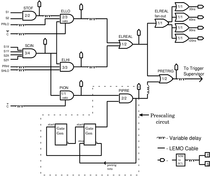
Figure 2.37: HMS/SOS single arm trigger electronics.

2.7.1 Hodoscope

Each hodoscope plane consisted of 9-16 individual elements, each of which was read out on both sides (the ‘positive’ and ‘negative’ ends). The signals from the tubes were discriminated and the tubes from the positive (and negative) ends were ORed together to give the signals S1X+, S1X-, $\ldots$. A hit in a given plane was defined as a coincidence of a hit in one of the positive tubes and a hit in one of the negative tubes, (e.g. S1X $\equiv$ [S1X+] + [S1X-]). This definition does not require both tubes to be on the same scintillator, but requires much less electronics and does not cause any significant amount of random signals. Two scintillator triggers are then formed. ‘STOF’ was defined as the coincidence of one of the front planes and one of the back planes, which is the minimum hit requirement for a good time of flight measurement in the scintillators. ‘SCIN’ required that 3 of the 4 planes fired, and provided a tighter scintillator trigger. Since any combination of three planes will include one S1 plane and one S2 plane, every time SCIN was true, STOF was also true. Occasionally, a PMT would be lost due to a failure in the high-voltage for that channel or a problem with the PMT base. Each plane has an average efficiency of $\sim$99.9%, and so even when a PMT is lost, the trigger efficiency for events passing through that scintillator is still $\sim$99.7%. There were no cases where multiple PMT signals were missing in the trigger electronics. The only cases in which two or more PMT signals were lost involved either a problem in the electronics (after the trigger signal is formed) or else a failure in the PMT base that affected the ADC, but not the discriminated signals used in the trigger. This problem occurred when an anode solder connection broke in such a way that it become AC-coupled. This meant that no charge could flow across the connection, but that the signal could still be large. This gave a distorted pulse shape with a very narrow negative voltage spike followed by a narrow positive spike. However, the signal is still able to fire the discriminator, which generates the trigger and TDC signals. Therefore, the ADC signals were lost, but there was no significant inefficiency in the hodoscope trigger. Finally, for an event with both a good Čerenkov and shower counter signal, the ELLO trigger (see next section) will fire on the STOF hodoscope condition. Therefore, even if a plane was missing completely, the trigger could still fire with one front and one back hodoscope hit as long as both particle identification signals were present. The necessary Čerenkov and shower counter signal were both $\mathrel{\raise 1.29167pt\hbox{$>$}\mkern-14.0mu\lower 2.58334pt\hbox{$\sim$}}98\%$ efficient for all except the lowest momentum settings in the SOS, so in general the STOF signal (two hodoscope planes) was sufficient to generate a trigger.

2.7.2 Electron Trigger

Because of the high pion to electron ratio for some of the kinematic settings, we require the event to pass some particle identification cuts before generating a trigger. In order to have a high efficiency for detecting electrons, we accepted a trigger as an electron if either the Čerenkov fired or if the calorimeter had a large enough signal. This allows an extremely high electron efficiency even if one of the two detectors has a low efficiency, but limits our hardware pion rejection. The Čerenkov signal used in the trigger (CER) was true if the Čerenkov sum fired the discriminator, set at between one and two photoelectrons. The shower counter signals had discriminators on the total (hardware) sum of all blocks (SHSUM) and the sum of all blocks in the first layer (PRSUM). The total energy had one discriminator threshold (SHLO) and the pre-radiator had one discriminator with a high threshold (PRHI) and one with a low threshold (PRLO). The final electron trigger (ELREAL) was the OR of the two conditions. ELHI required a high calorimeter signal, but no Čerenkov signal, while ELLO required a Čerenkov signal, but not a calorimeter signal. ELHI was defined as the coincidence of SCIN, PRHI, and SHLO (a tight scintillator cut and both a high pre-radiator sum and total energy sum from the calorimeter). ELLO required the Čerenkov signal (by vetoing with the $\overline{CER}$ signal) as well as two of the following: a tight hodoscope condition (SCIN), a loose hodoscope condition (STOF), and a shower counter signal (PRLO). If the SCIN signal (3/4 hodoscope planes) is present for an event, there must also be a STOF signal (which requires one front plane and one back plane). This means that ELLO requires the Čerenkov and either the ‘good’ scintillator trigger (SCIN), or the minimum scintillator trigger (STOF) and the lower shower counter signal (PRLO).

2.7.3 Pion Trigger

There was also a pion trigger that allows a sample of the pions to be taken in order to study the pion background. The raw PION signal was defined as a good hodoscope trigger (SCIN) vetoed by the CER signal (note that this is not mutually exclusive with the electron trigger). This PION trigger was prescaled using a dynamic prescaling circuit, and the prescaled pion triggers, PIPRE, were ORed with the ELREAL signal to give the final HMS or SOS singles trigger. The prescaling was accomplished using two gate generators, where each one was opened when the other closed. Thus, the two gates toggle on and off, and pion triggers were passed only when the second gate was open. Whenever a pion trigger was accepted, the second gate was closed. Since the second gate remains closed whenever the first gate is open, the width of the first gate sets the minimum time between accepted pions, and therefore the maximum rate of accepted pions. The maximum pion rate and the minimum prescaling factor can be set by varying $\tau_{1}$ and $\tau_{2}$, where $\tau_{1}$ is the gate width for the first gate generator, and $\tau_{2}$ is the width of the second gate. If the pion rate is very high, a pion will be taken as soon as the second gate opens and all others will be blocked until a time $\tau_{1}$ has passed, and the maximum pion rate is $R_{\pi}^{max}=1/\tau_{1}$. If the pion rate is very low, the second gate will usually stay open for its set width, and the fraction of the time that pions is accepted is equal to $\tau_{2}/(\tau_{1}+\tau_{2})$. Therefore, by setting $\tau_{2}\gg\tau_{1}$ and $1/\tau_{1}=R_{\pi}^{max}$, the prescaling circuit will allow virtually all pions at very low rates, $R_{\pi}^{max}$ at very high rates, and something in between for all other cases. For e89-008, the particle identification provided by the calorimeter and Čerenkov was sufficient to reject the pions, making subtraction of the pions unnecessary. Taking prescaled triggers makes it more difficult to use the hardware scalers as an online diagnostic, and so the pion trigger was disabled for the bulk of the data taking in e89-008.

2.7.4 Other Signals

In addition to providing the information used in the trigger, all of the intermediate signals are sent to scalers and TDCs. The TDCs are mainly used as latches, and tell which signals were present when the trigger was taken. This allows us to determine what kind of event formed the trigger. The scalers allow us to look at raw rates and look for certain types of electronics problems in the intermediate steps of trigger formation. We also use the scalers to measure computer and electronics dead time by comparing the number of triggers that were formed with the number that were accepted (see section 3.3.5).

2.7.5 Data Rates

The maximum data taking rate is limited by the fastbus conversion and data readout time. In basic data acquisition mode, the total time to process an event is just under 1 ms. The time is broken up as follows: $\sim 95\mu$s for fastbus data conversion, $\sim$150 $\mu$s for the fastbus crate controller (FSCC) to read the data from the ADC modules into it’s FIFO, and $\sim$650 $\mu$s for the FSCC to take the data from it’s FIFO into memory and send it out over ethernet. This limits data acquisition to $\sim$1.1 kHz, but gives large computer dead times even at lower rates. Several improvements have been made to improve the data rate and decrease dead time. First, because the FSCC is inefficient at sending data over the ethernet, the readout of the fastbus data was modified so that when running in ‘parallel’ mode, the data was read out from the FSCC FIFO through a VME CPU. This reduced the processing time to $\sim$95 $\mu$s for fastbus conversion, and $\sim$400 $\mu$s for the data readout. In addition, optimization of the fastbus readout of the TDCs and ADCs reduced the fastbus readout time to 300 $\mu$s, giving a total time to process the event of $\sim$400 $\mu$s and a trigger rate limit of $>$ 2 kHz when running in parallel mode. However, the dead time is still large for rates well below this limit. The fraction of events missed is equal to the fraction of the time the computer is busy which equals the rate of events taken over the maximum rate (2-2.5 kHz), so even at 500 Hz the computer dead time is $\sim$20-25%. In addition to the improvements gained by running in parallel mode, the fastbus modules we use allow buffering of 8 events. This allows the trigger supervisor to accept new triggers as soon as the fastbus conversion is done, rather than waiting for the full conversion and readout time. This means that the dead time is roughly one quarter of what it is in non-buffered mode. The total processing time for an event is still $\sim 400\mu$s, so the total event rate limit does not improve, but fewer events will be missed for rates lower than the maximum. Figure 2.38 shows the expected dead time (fraction of triggers that are missed) versus the trigger rate for the basic, parallel, and parallel buffered modes. Figure 2.39 shows the measured dead times for runs taken in the parallel buffered mode.

Figure 2.38: Expected data acquisition dead times for standard(dotted), parallel link(dashed) and parallel buffered(solid) run types as a function of incoming event rate.

Figure 2.39: Data acquisition dead times for runs taken using parallel buffered mode. The solid line is the expected deadtime assuming a 95 $\mu$s trigger processing time. Note that because of buffering, the dead time is below 20% for incoming event rates up to 2.5kHz, even though the maximum rate at which data can be taken to disk is $\sim$2.5 kHz.

For a handful of runs, there was a problem in the synchronization between the drift chamber TDCs and the hodoscope, Čerenkov, and calorimeter ADCs and TDCs. This happened when excessive ‘noise’ caused extra triggers to appear at the fastbus crate containing the drift chambers. In buffered mode, each crate digitizes and stores up to 8 events. If an extra trigger comes to the crate, it will perform an extra read. Because the individual TDC stop signals are not present, it will tag the data for this read as being incomplete. However, it is stored in the buffer and not read out until a real trigger causes the event builder to read the data from each crate. The TDC readout caused by the bad trigger will take the place of the TDC readout caused by the current trigger. After this point, the drift chamber events are always being read out with data from the previous event, or data from earlier events, if the noise caused multiple false triggers. Because this affected only a very small part of the data, the runs where there was a synchronization problem were discarded.

2.8 Data Acquisition

The data files for the runs contain both event information and slow controls readout. These two types of information were read out separately. CODA (the CEBAF Online Data Acquisition system) was the data acquisition system developed by the data acquisition group at CEBAF and used for this experiment. Information on CODA and RunControl (a graphical user interface) can be found in refs. [58, 59]. The system in place for Hall C experiments is shown in figure 2.40 and described in reference [60]. There are three main types of events: status events that have information about the run, physics events that contain data read out from events in the spectrometer, and EPICS (Experimental Physics Industrial Control System [54]) events which have readout from slow controls. The experiment took a total of $\sim$100 Gb of data.

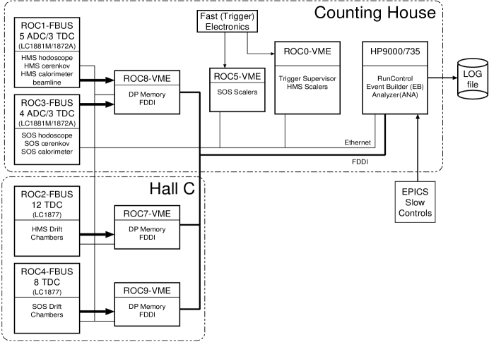
Figure 2.40: Schematic of the Hall C data acquisition system.

2.8.1 CODA Overview

Data acquisition in Hall C is broken up into several pieces, which are controlled by the CEBAF Online Data Acquisition (CODA). The data is read out from Read-Out Controllers (ROCs). In our setup, the ROCs are CPUs in Fastbus and VME crates in the hall and in the electronics room. These crates contain the ADCs, TDCs, and scalers that contain the event information. The Trigger Supervisor (TS) controls the state of the run, and generates the triggers that cause the ROCs to be read out. The Event Builder subsystem (EB) is the part of CODA that reads in the data fragments from the ROCs and puts the data together into an event, incorporating all of the necessary CODA header information needed to describe and label the event and the data fragments. CODA manages the data acquisition system, and takes care of handling the data from the events. After the event is built by the EB, it is placed into a buffer, after which it can be tested (and rejected if desired), analyzed, or sent to disk or tape. For our run, data was directly sent to disk and analyzed by separate processes after it was saved. In addition to running the data acquisition, CODA also includes a graphical user interface (RunControl) which allows the user to start and stop runs, as well as define run parameters.

2.8.2 Status Events

The first events in the log file for each run are a series of status events. There are prestart, start, pause and end events that are included whenever the state of the run changes. In addition, there are several user defined status events. At the beginning of the run, the user can enter information about the run (kinematics, magnet settings, comments) in a Tk/Tcl window. This information is stored in a special beginning of run event. In addition, at the beginning of the run, there are status events that record the ADC threshold values that were programmed in at the beginning of the run. This allows the analysis software to compare the set thresholds to the desired values, as determined by the pedestal events.

2.8.3 Physics Events

For our experiment, the spectrometers gave independent triggers, and the physics events contained data for only one spectrometer (along with some event-by-event beamline information). The TDCs were operated in sparsified mode, so that only channels with stops were read out. The LeCroy 1881M ADCs had programmable thresholds for each channel, allowing sparsified readout of the ADCs as well. The thresholds were typically set at 15 channels above the pedestal, and 1000 random triggers were generated at the beginning of the run (with sparsification disabled) in order to measure the centroids and widths of the pedestals. In addition to the spectrometer information, some beam related quantities were read out on an event-by-event basis. Beam position monitors, beam loss monitors, and beam raster readback values were recorded for each event. Typical event sizes for single spectrometer readout with sparsification enabled were $\sim$400-500 Bytes/event, which corresponds to a data rate of $\sim$1 Megabyte per second for the maximum event rate of 2-2.5 kHz. As this was slightly below our maximum data rate, it was not necessary to limit the event size or improve the data flow rate.

2.8.4 EPICS Events

In addition to the physics events, other user event types can be defined in CODA, allowing readout of hardware scalers or execution of user scripts. Readout of the hardware HMS and SOS scalers was triggered every two seconds by an asynchronous process. Slow controls (detector and beamline controls and readout not directly associated with data acquisition) were read out by a script triggered by CODA every 30 seconds. CEBAF uses an EPICS database as it’s interface to the accelerator and much of the Hall C instrumentation. Values such as spectrometer magnet settings, accelerator settings, and target status variables were accessed this way. In addition, independent processes logged target and magnet status information.

Chapter 3 Data Analysis

3.1 Event Reconstruction

The analysis of the raw data files was done using the standard Hall C event reconstruction software. The event reconstruction code reads the raw events, decodes the detector hits, and generates tracks and particle identification information for each event. In addition, it keeps track of the hardware scalars and generates software scalers for the run. The detector calibrations were done using separate code and the results were taken as input to the event reconstruction software. The data is output in three forms. Report files contain the hardware and software scalars, as well as calculated detector efficiencies. PAW [61] HBOOK files contain the standard set of histograms which can be used to check detector performance and monitor the hardware during a run. PAW Ntuple files contain the event by event information, and are the main output used in the final physics analysis. Histograms and Ntuples are generated using the CERN HBOOK libraries. Input parameters, software scalars, histograms and tests are handled using the CEBAF Test Package (CTP) [62], which was written at CEBAF, and is modeled loosely on the LAMPF Q system [63]. After the tracking, efficiency, and particle identification information is generated by the analysis package, The physics analysis is done using separate stand-alone Fortran and PHYSICA [64] code.

Sections 3.1.1 through 3.1.3 describe the tracking algorithm, time of flight measurement, and particle identification (PID) information. A detailed description of the analysis code is given in appendix A. Section 3.2 describes the detector calibration procedures.

3.1.1 Tracking

The trajectory of the event at the focal plane is measured with two drift chambers, each with six planes. The position of the track as it passes through a plane is determined by starting at the position of the wire that detects the particle, and adding the distance of closest approach between the track and the wire. This distance is determined by measuring the time difference between the time that the particle passed through the focal plane (as determined by the scintillators) and the time at which the wire detected the particle passing. It is assumed that the particle is moving nearly perpendicular to the plane, and that the point of closest approach is in the plane of the drift chamber. In addition, small corrections are applied for the time required for the signal to propagate along the wire and differences in cable lengths from between the chamber and the Time-to-Digital Converters (TDCs).

The drift chamber hits are used to identify clusters of hits (space points) in the front chamber. The drift time is determined from the drift chamber TDC values and the hodoscope start time. For each space point, a ‘stub’ is fit. This is a track determined using just the hits in the first chamber. For each wire in a space point, the particle could have gone past the wire on the left or the right. The left-right determination can be made by fitting a stub through the space point for each left-right combination ($2^{6}$ stubs per space point) and choosing the stub with the lowest $\chi^{2}$. However, in order to improve the speed of the tracking algorithm, we use a small angle approximation for the $y$ and $y^{\prime}$ planes in the HMS (High Momentum Spectrometer), and all of the planes in the SOS (Short Orbit Spectrometer). In the $y$ and $y\prime$ planes (or any two parallel planes), the wires within each plane are separated by 1 cm, but the parallel planes are offset 0.5 cm. If you have a hit in both planes, you can choose the left-right combination that makes the particle go between the wires. For planes that are close together and incoming particles that are nearly perpendicular to the drift chambers, this is a very good approximation. Therefore, a space point with one hit in each of the six planes has only $2^{4}$ possible left-right combinations in the HMS (since the left-right determination for the $y$ and $y$’ planes is made using the small angle assumption), and no left-right ambiguity in the SOS. Approximately 3$\%$ of the time, a plane is missing and the left-right determination for its partner plane is made by looping through all $2^{5}$ possible left-right choices that are not determined by the small angle assumption and choosing the stub with the lowest $\chi^{2}$. After all space points have been found in the front chamber, and stubs fit for each one, the code finds space points and stubs for the second chamber. Finally, for each combination of stubs in the front and back chambers, a full track is fit if the two stubs were consistent (i.e. the slopes of the stubs must be consistent, and they must point to each other). Each of these tracks is recorded along with the $\chi^{2}$ of the fit.

In bench tests, the HMS and SOS chambers had resolutions of $\mathrel{\raise 1.29167pt\hbox{$<$}\mkern-14.0mu\lower 2.58334pt\hbox{$\sim$}}$150 $\mu$m per plane. However, in the final two-chamber tracking, there are additional resolution effects coming from the resolution of the start time from the hodoscopes, wire position offsets or wire sagging, and errors in the drift chamber position or angles. By comparing the position measurements of the individual planes and comparing them to the final fitted track, we obtain a tracking resolution of $\sim$280 $\mu$m per plane in the HMS, and $\sim$180 $\mu$m in the SOS. For the HMS, each chamber has two planes that measure $y$, and four planes that primarily measure $x$. This gives a position resolution in $x$($y$) of $\sim 140\mu m$ ($200\mu m$) and an angular resolution of 0.24 mr for $\frac{dx}{dz}$ and 0.34 mr for $\frac{dy}{dz}$. The resolution on the momentum and reconstructed angles is given in table 2.6 and is a combination of the drift chamber resolution and the error in the track reconstruction. The resolution on the reconstructed quantities is worse at lower electron energy as multiple scattering in the target, scattering chamber, and magnet entrance window. At low momentum spectrometer momentum settings, the multiple scattering dominates the resolution. For the SOS, there are six measurements per plane, with equal $x$ and $y$ information, giving a position resolution of $\sim$ 105 $\mu m$ and an angular resolution of $\sim$0.30 mr. Note that while the position resolution is better in the SOS, the angular resolution is comparable in the two spectrometer because the SOS chambers are separated by 49.5 cm, while the HMS chambers are separated by 81.2 cm.

Before a fitted track is accepted as a good track, cuts are applied to reject bad fits caused by space points with missing wires or with noise hits. The track is used to determine which hodoscope elements and which calorimeter blocks the particle passed through, and cuts are applied on the particle velocity, the signal in the calorimeter, and the measured dE/dx in the hodoscope, all as measured using the detector elements that lie on the fitted track. In addition, a hard cut is placed on the $\chi^{2}$ of the fit for the track. If multiple tracks pass these cuts, then the track with the best $\chi^{2}$ is selected as the final track. In our analysis, the hard cuts were opened up, allowing all good tracks to pass, and the best track was selected using $\chi^{2}$. Typically, multiple tracks are found in 1-2$\%$ of events (3$\%$ worst case). Most of these tracks come from finding space points with slightly different sets of wires. Typically, 5 of the wires occur on both tracks, and only the sixth differs (or is missing). In these cases, the tracks are nearly identical, and the choice of the lower $\chi^{2}$ is effective in selecting the appropriate track when one of the hits is a ‘random’ hit. The fraction of events with true multiple particles in the spectrometer is typically less than 0.1$\%$, and is always less than 1$\%$.

3.1.2 Hodoscope Timing Measurements

The time of flight (TOF) of the particle through the spectrometer is determined for each track found in the drift chambers. Different tracks could point to different scintillators, and only those scintillator hits consistent with the track are included in the TOF measurement. For each scintillator on the track, the TDC values are converted to nanoseconds. A correction is applied for the pulse-height walk, time of propagation through the scintillator, and cable length offsets between the different photomultiplier tubes (see section 3.2). For each scintillator, the times from the two PMTs are combined if there are two hits to give a time for each scintillator. If there is at least one time in the front hodoscope and one in the back, the velocity is calculated for the track using the $z$ position of the hodoscopes, the time for each scintillator, and the angle of the track. Given the velocity of the particle and the momentum (from tracking), the particle mass can be determined, and slow particles can be identified. During e89-008, the spectrometers were looking at negative particles, and the momentum was too high to differentiate pions and electrons using time of flight. However, for the positive polarity runs used to measure the charge-symmetric background (see section 3.3.4), the time of flight was used to verify that there were no protons remaining after the other PID cuts.

In addition to using the hodoscope times to calculate the time of flight for the particle, we also use the hits to determine the time at which the electron passed through the drift chamber. This is subtracted from the TDC value for the individual wire hits in order to determine the drift time which is needed to determine the distance between the particle and the wire as it passed through the chamber. Because this time must be determined before a track has been found, we cannot correct for the time delay caused by the signal propagating from the position of the hit to the PMT. Therefore, we require that both PMTs on the hodoscope paddle fire. If both PMTs give a good time measurement, the velocity corrections for the two PMTs will cancel each other and the mean time will be independent of the position of the hit.

3.1.3 Particle Identification

For many of the e89-008 kinematics, there was a large pion background, sometimes up to 100 times the electron rate. Loose cuts on the gas Čerenkov detector and lead-glass shower counter were used to reject pions in the trigger, and tighter cuts were applied in the offline analysis. The cuts used and their efficiency are discussed in section 3.3.3.

The Čerenkov consisted of four mirrors and PMTs in the SOS, and two in the HMS. In both cases, the Analog-to-Digital Converter (ADC) output from each PMT was converted into the number of detected photoelectrons. The Čerenkov signal for the event is just the sum of the signals from the phototubes. No corrections were applied for position dependence of the signal, but the cuts were chosen to give high efficiency over the entire acceptance of the spectrometer.

For the calorimeter, one ADC value is measured for each module. The ADC value is converted to energy deposited in the block in GeV. Clusters of hits are located, and the energy per layer and total energy is calculated for each cluster. For each track found by the drift chambers, the energy associated with that track is the energy of the cluster that the track points to, if there is one. The energy is corrected for attenuation in the blocks based on the distance of the hit from the PMT, as determined by the tracking.

3.2 Detector Calibrations

Calibrations had to be performed in order to match the timing of the individual scintillator elements, to calibrate the gains of the calorimeter and Čerenkov PMTs, and to convert the drift chamber TDC values to drift distances. For the gas Čerenkov, the final gains were calculated by hand. For each PMT, one gain parameter was needed; the number of ADC channels per photoelectron. The pedestal values were subtracted from the ADCs, and the gains were determined by finding the one photoelectron peak or by comparing the mean and widths of the signal in a central region. The drift chambers, hodoscopes, and calorimeter had a more complicated calibration procedure that involved running the tracking code and saving information for many events, and then fitting for the corrections using stand-alone code.

3.2.1 Drift Chamber Calibrations

The drift chambers provide a list of hits for each event, along with a TDC value for each hit. Using the hodoscopes to determine the time that the particle passed through the focal plane, the drift chamber TDC values can be converted into a drift time. In order to determine how far the track was from the wire, we generated a time-to-distance map using the following procedure. First, we take the TDC values from all of the wires in a given plane for a large number of events (at least 50k). This gives us the drift time distribution. We assume that after averaging over all cells, the drift position distribution is uniform. After applying a loose cut to reject random ‘noise’ hits, we integrate the time spectrum. The drift distance is then just

$$D=D_{max}{{\int_{t_{min}}^{T}F(\tau)d\tau}\over{\int_{t_{min}}^{t_{max}}F(\tau)d\tau}},$$ (3.1)

where $t_{min},t_{max}$ define the range of times to be included in the fit, $D$ is the distance from the wire, $D_{max}$ is the maximum possible distance (1/2 of the wire spacing, or 0.5 cm), $F(\tau)$ is the drift time distribution, and $T$ is the time value from the TDC. In reality, the distribution over a single cell is very non-uniform. However, when the cells are combined, the deviations from uniformity are small enough that the effect on the drift distance reconstruction is on the order of 10 $\mu$m, well below the resolution of the chambers. A separate time-to-distance map is generated for each plane in the chambers. Figure 3.1 shows the measured drift time distribution for one of the $y$ planes, along with the drift distance calculated from the drift time.

Figure 3.1: Drift time and drift distance spectra for the HMS drift chamber. Drift times between -24 ns and 252 ns are mapped into a uniform distribution of drift distances over the half cell size. Note that the first and last bins only partially overlap the 0.5 cm region, and therefore contain less than the other bins. The drift time can be negative because the overall offset between the times measured by the drift chamber and the time measured by the hodoscope is not removed.

The final resolution for the drift chambers was $\sim$280 $\mu$m per plane in the HMS and $\sim$180 $\mu$m per plane in the SOS. A single time-to-distance map was used for all runs. Due to small long term drifts in the electronics, temperature variations, and rate dependence in the chambers, the resolution could have been improved somewhat by using different time-to-distance maps for runs taken at different times or at vastly different event rates. In addition, because the hodoscope provides the drift chamber start time, a more careful calibration of the hodoscope timing could have made a small difference in the resolution. However, the resolution would be improved only 10-20%, and the current resolution is sufficient for e89-008.

3.2.2 Hodoscope Timing Corrections

There are several corrections that need to be made in order to convert from the TDC value of the hit to the time of the hit. Once the particle passes through the scintillator, the light has to propagate through the scintillator until it reaches the phototube. The signal travels through about 500 ns of cable to get to the electronics in the counting house. After passing through a series of discriminators and gates, the signals are then fed to TDCs to measure the time of the event. All of the delays introduced between the event and the final TDC measurement must be corrected for in order to reconstruct the time of the event. Bench tests indicated the the scintillators had a mean time resolution of $\sim$70-100 ps, and so timing corrections had to be carefully fit to achieve a final resolution near this limit. Fortunately, only a relative time between the scintillators need be determined. The overall time it takes to reach the TDC is not important.

The first step in the calibration process was to check the scale (ps/channel) of the TDCs. The linearity of the TDC scale (ps/channel) was determined by testing the TDCs using an ACL-7120 Time Interval Generator. The absolute time scale was verified with the accelerator RF signal (499 MHz), using the prescaled RF as the TDC start, and the raw RF as the TDC stop. This gives a series of peaks separated by 2.004 ns. The calibration of the modules differed from the nominal values by up to 6%, but channel to channel variations within a module were on the level of 1-2%. When we fit the timing corrections for each signal, an arbitrary time offset is included. Therefore, the error due to channel to channel variations is 1-2% of the range of TDC values for that channel. Even though the TDC had a full range of 100 ns, the TDC value for a single signal would typically vary over a range of less than 10 ns. Therefore, a 2% variation in the time scale for the different channels will only cause $\pm$25 ps channel to channel timing variations. Since this is significantly better than the intrinsic resolution of the hodoscopes, the TDC scale for each set of hodoscopes was set to the average value for the entire TDC, and no channel to channel correction was applied.

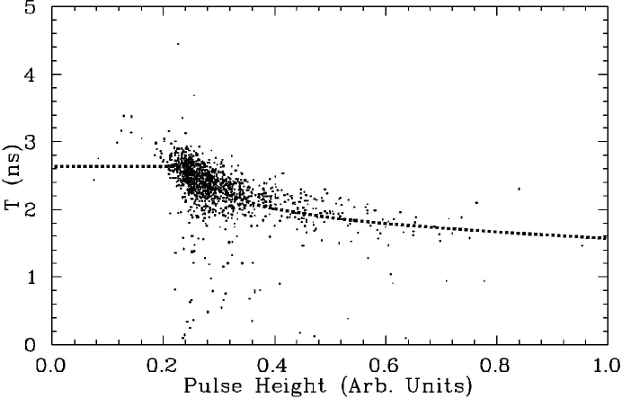
Figure 3.2: Time (relative to start time) from PMT versus pulse height (as determined from the ADC) for events in a small region of the scintillator.

Once the calibration for the TDCs has been determined and the TDC value converted into a time, corrections have to be made for timing variations caused by signal pulse height variations, light propagation time in the scintillators, and overall timing offsets between the individual signals. Because the timing signal comes from a fixed threshold discriminator, the time between the start of the signal and the time that the threshold is exceeded depends on the height of the signal. Thus, large signals will fire the discriminator earlier than small signals. These corrections are hundreds of picoseconds, and have a significant effect on the resolution of the scintillators. If we take hits in a small region of one of the scintillators (to minimize corrections due to light propagation in the scintillator) and compare the time from that PMT hit to the average of all scintillator hits, we can clearly see the variation of timing with pulse height (see figure 3.2). However, this effect is diluted by the fact that the averaged time varies due to pulse height walk in the other scintillators. To fit the correction, we take crossed pairs of scintillators to limit the region of the scintillator that is hit and compare the mean times of the elements (the mean time is the average of the times measured by the PMTs on each end). Taking the mean time eliminates the dependence on position along the scintillator, and leaves only the pulse height correction and an overall offset. By applying a rough correction to the pulse height walk in three of the four PMTs, the remaining dependence on the ADC value of the uncorrected tube gives a measurement of the corrections due to pulse height variations. We use a correction of the form:

$$\Delta t=PHC*\sqrt{max(0,(ADC/PHOFF-1))}+t_{0},$$ (3.2)

where ADC is the raw ADC value, and PHC, PHOFF are the timing correction parameters, and $t_{0}$ is an arbitrary offset between the two scintillators.

Once the pulse height correction is known, the velocity of light propagation along the scintillator element can be measured by taking the difference in times of PMTs on the opposite ends of an element. When plotted versus position along the scintillator, the velocity of propagation can be determined by the slope. Note that this velocity is not just the speed of light in the plastic scintillator, because most of the light bounces off of the sides of the scintillator, rather than going directly towards the PMTs. The velocity correction therefore depends on both the index of refraction and the cross section of the scintillator. A velocity was measured for each plane, and all elements in that plane used this average correction. Finally, each tube has its own time offset due to variations in cable length or different response times of the PMTs. These are fit in the same way as the pulse height corrections. The mean time is generated for a pair of scintillators, with velocity and pulse height walk corrections made. The offsets are adjusted in order to make the time between the scintillator hits agree with the known velocity of the particle ($\beta$=1 for electrons, and $\beta$ as calculated from the momentum of the particle for hadrons).

Figure 3.3: HMS time of flight and timing resolution. The figure on the left is the distribution of measured velocities, $\beta=v/c$. The figure on the right is a distribution of the standard deviation of the focal plane time measurements from the different hodoscope planes. For each hodoscope element on the track, a focal plane time is determined. From these (three or more) time measurements, the standard deviation is calculated.

Figure 3.3 shows the final timing resolution for the HMS. The reconstructed $\beta$ spectrum is shown, along with the standard deviation of the focal plane time measurements from all hodoscope elements that had a good time measurement. For the SOS, the width of the gaussian fit to the $\beta$ peak was identical, but the tails at low $\beta$ were slightly smaller and the average $\sigma$ at the focal plane was 110 ps (median 95 ps). The hodoscope planes in the SOS are separated by $\sim$180 cm, while the HMS hodoscope planes are $\sim$220 cm apart. Therefore, while the SOS has a better timing resolution, the resolution in $\beta$ is identical for the two spectrometers. In both cases, the width of the gaussian fit to the $\beta$ spectrum is the value expected from the timing resolution of the individual hodoscope elements. However, there are noticeable tails in the $\beta$ spectrum. This occurs because a few elements have very poor statistics in the runs used to fit the correction parameters. Because of this, we fit the corrections for each PMT, but use only one set of velocity and pulse height correction coefficients per plane. This helps to prevent getting unreasonable correction parameters for elements with low statistics in the fitting run, but does not take into account element to element variations caused primarily by different distributions of hits over the length of the scintillators. It is possible to improve the tails by checking the fitted values for elements, being careful to avoid poor fits for elements with low statistics. For e89-008 we are not interested in using the time measurements for hadron rejection because pions cannot be cleanly separated from electrons at the values of momentum where we have data. The hodoscope times are needed to generate a start time for the drift chambers, but only require sub-nanosecond resolution, and the tails are well below this level. The drift velocity of the electrons in the drift chamber is roughly 50 $\mu$m/ns, and the intrinsic chamber resolution is $\sim$150 $\mu m$, so nanosecond level variations in the start time have a relatively small effect on the chamber resolution.

3.2.3 Lead Glass Calorimeter Calibrations

In order to determine the energy deposited in the calorimeter, the gain of each module (lead glass block plus PMT) must be determined, and the ADC value measured must be converted into an energy deposited. This measured energy must also be corrected for attenuation in the lead glass block. Attenuation in the lead glass gave a variation of signal with distance from the PMTs, since each block was only read out on one end. To correct for the attenuation, the signal from each block was multiplied by a correction factor based on the hit position. This correction was checked by looking at the distributions of measured energy as a function of distance from the PMTs. Figure 3.4 shows the measured calorimeter energy versus y position (y=0 corresponds to the center of the block) before and after the correction for attenuation. Note that the conversion from ADC channels to Energy (GeV) was determined for a hit in the center of the blocks. Therefore, the attenuation correction corrects the measured energy to the value at the center, rather then raising the signal everywhere to remove the attenuation.

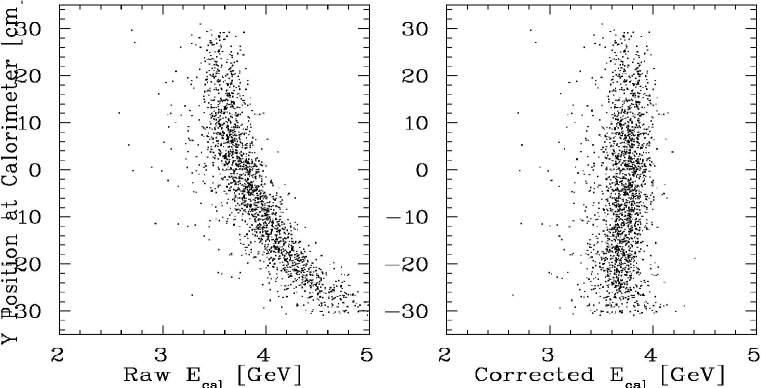
Figure 3.4: HMS Calorimeter

In addition to correcting for attenuation, it is necessary to correct the gains of the individual modules. Electron data was taken, and the operating high voltage values for the calorimeter PMTs were adjusted so that the ADC signal was identical (to $\sim$10%) for blocks in the same layer. Electrons with larger momenta will be bent less in the spectrometers, and will populate the bottom blocks in the calorimeter. Because the bottom blocks are detecting higher energy electrons, their gain must be lower than the top blocks so that the output signals will be of the same size. Therefore, setting the gains such that the output signal is constant as a function of position in the calorimeter means having a gain variation between the blocks roughly equal to the momentum acceptance of the spectrometers ($\sim$20% in the HMS, $\sim$40% in the SOS). The output signals were made equal (rather than the gains) in order to make the calorimeter trigger efficiency as uniform as possible over the entire calorimeter.

In the final data analysis, the ADC signals had to be converted into measured energies, and the signals had to be corrected to the few percent level. In order to correct for the gain differences of the lead glass modules, we select good electron events using the Čerenkov, and record the pedestal subtracted ADC values for each block, along with the energy of the electron as determined from the track reconstruction. The gain correction factor for each block is varied in order to minimize the difference between the energy sum from all blocks and the true energy of the electron. Because electrons deposit most of their energy in the first two or three layers, this procedure is not very reliable for calibrating the last layer of the calorimeter. Pions, which generally deposit the same energy ($\sim$60 MeV) per layer from ionization, are used to calibrate the last layer of the calorimeter. The calibration coefficients for the last layer are determined by using a Čerenkov cut to generate a clean sample of pions, and matching the energy deposition in each block of the last layer. For the third layer of the calorimeter, the electron energy deposition is fairly small except for the highest energy electrons. Therefore, the calibration based on electron energy distributions can be somewhat unreliable, especially at low electron energy or in regions of the calorimeter where there are fewer events. Because of this, the pion energy deposition was used as a check of the calibration in the third layer, and a few gains (mostly near the top and bottom of the calorimeter) were modified.

After the blocks have been calibrated, and the measured energies corrected for attenuation, the resolution, $\delta E/E$, is 5.6%/$\sqrt{E}$ for the SOS, and 6-8%/$\sqrt{E}$ for the HMS (E in GeV), as shown in figure 2.36. The intrinsic resolution of the HMS calorimeter is $\approx$ 6%/$\sqrt{E}$, but for approximately half the data, the ADC pedestals had small fluctuations, and the resolution was worse (see section 3.3.3 for details). A single set of calibration constants was generated for the HMS calorimeter and was used for all runs. Figure 3.5 shows the difference between the energy measured in the calorimeter and the HMS momentum. Over the entire range of momenta used, the measured energy agrees with the expected value to $\mathrel{\raise 1.29167pt\hbox{$<$}\mkern-14.0mu\lower 2.58334pt\hbox{$\sim$}}3\%$. For the SOS, two sets of calibration coefficients were used because of a high-voltage supply change near the end of the run. The measured energies agreed with the detected momenta to better than 3% over the entire run, for momenta between 0.7 and 1.7 GeV/c.

Figure 3.5: HMS measured calorimeter energy as a function of spectrometer momentum.

3.3 Extraction of ${\bf d\sigma/d\Omega/dE^{\prime}}$

The Hall C event reconstruction code provides tracking and particle identification (PID) information for each event. It also measures detector efficiencies and analyzes information from the scaler readouts used to measure the total beam current for the run and to determine the deadtimes and efficiencies needed to generate an absolute cross section from the measured counts. The analysis code is described in detail in appendix A. After the run has been analyzed, separate analysis code applies tracking and particle identification cuts and detector efficiency corrections. In addition, several corrections must be applied to convert between measured counts and cross section. The counts must be corrected for spectrometer acceptance, dead time in the data acquisition, and inefficiency in the hardware trigger, tracking algorithm, and cuts. The measured beam current and target thickness is used to convert the measured counts to cross sections. In order to extract the physics cross section, the measured cross section must be corrected for radiative effects.

3.3.1 Pre-reconstruction Cuts.

Before the events are reconstructed, the TDCs that record the intermediate trigger signals are examined, and events are rejected unless they contain both a Čerenkov signal (CER) and a shower counter signal (PRLO, SHLO, or PRHI). See section 2.7.2 for the definition of the trigger signals. This effectively modifies the online trigger from an OR of the two detectors to an AND. The shower counter signal required in the calorimeter based trigger (ELHI) sometimes has an electron efficiency as low as 90% (at the lowest momentum settings). However, it requires that the total energy be above a fixed threshold (SHLO) and that the energy in the first layer be above a fixed threshold (PRHI). It is this ‘high’ threshold on the first layer energy that causes most of the inefficiency for electrons in the ELHI trigger. By requiring only one of the three signals (SHLO, PRHI, or PRLO, which is a lower threshold on the pre-radiator energy), the efficiency becomes very high ($>$99%).

This offline ‘trigger modification’ is done for two reasons. First, in order to insure that the trigger efficiency would be high even if one of the detectors was not working well, the thresholds were set relatively low. This limited the online pion rejection. By modifying the trigger requirements before reconstructing the event, we can reduce the size of our data set by a factor of two. This significantly reduces the time required to analyze the data set.

In addition to reducing the data set, this cut has an additional benefit in the SOS. In the SOS Čerenkov signal, there was significant noise in the ADC readout which limits the offline pion rejection (see section 3.3.3). Because the noise was in the ADC, the trigger signal was not affected, and the pion rejection is not reduced. Therefore, we use a combination of the trigger signal (a $\sim$1.7 photoelectron on the clean signal) and a cut on the Čerenkov ADC (3.3 photoelectrons on the noisy signal). The online cut rejects pions at $\sim$250:1, and the offline cut rejects pions at $\sim$170:1. The combined efficiency is estimated to be between 300:1 and 380:1, and we assume 300:1 when estimating the pion contamination. The worst case pion contamination after the final particle identification cuts is $\sim$3%, and only occurs for the largest angle data, where the statistical uncertainties and systematic uncertainties due to other backgrounds are their largest ($>$10%).

3.3.2 Tracking Cuts

The event reconstruction code generates information for the tracks at the focal plane, and reconstructed tracks at the target. The focal plane quantities are the $x$ and $y$ positions and slopes of the track at the focal plane ($x_{fp},y_{fp},x^{\prime}_{fp}$,and $y^{\prime}_{fp}$), in the coordinate system defined in section 2.5.1 ($\hat{z}$ is parallel to the central ray, $\hat{x}$ points downwards, and $\hat{y}$ points left when viewing the spectrometer from the target). The reconstructed values are $\delta$, $y_{tar}$, $x^{\prime}_{tar}$, and $y^{\prime}_{tar}$, where $\delta=(p_{recon}-p_{0})/p_{0}$, with $p_{0}$ equal to the spectrometer central momentum, $y_{tar}$ is the horizontal position at the target plane (perpendicular to the spectrometer central ray), and $y^{\prime}_{tar}$ and $x^{\prime}_{tar}$ are the tangents of the in-plane and out-of-plane scattering angles, with $\hat{x}$ pointing downwards, $\hat{y}$ pointing left, and $\hat{z}$ pointing towards the spectrometer. Note that while $x^{\prime}_{tar}$ and $y^{\prime}_{tar}$ are the slopes of the tracks ($x^{\prime}_{tar}=\frac{dx_{tar}}{dz_{tar}}$), they are often referred to as the out-of-plane and in-plane scattering angles, and given the units of radians (or milliradians).

Cuts are applied to the reconstructed target quantities in order to eliminate events that are outside of the spectrometer acceptance but which end up in the detectors after multiple scattering in the magnets or shielding. The cuts are kept loose enough to avoid losing any real events due to the finite tracking resolution caused by the drift chamber position resolution and by multiple scattering in the target and the entrance and exit windows in the spectrometer. In addition, we apply a cut on the reconstructed momentum. This cut is applied so that we analyze data in the momentum region where we have good matrix elements for reconstructing the track to the target. The tracking cuts applied are listed in table 3.1.

In the HMS, the $x^{\prime}_{tar}$,$y^{\prime}_{tar}$, and $y_{tar}$ cuts typically rejected $\sim$1.0% of the total tracked events, and never more than 2%. Of these events, $80-90\%$ come from events that are outside of the acceptance, but scatter back into the detectors at the dipole exit or in the vacuum pipe afterwards. Therefore, the cuts are $>99.5\%$ efficient for good events. Of the events that scatter inside of the spectrometer and end up in the detector stack, $\mathrel{\raise 1.29167pt\hbox{$>$}\mkern-14.0mu\lower 2.58334pt\hbox{$\sim$}}$ 90% are rejected in the tracking cuts or with the background cuts (described later). More than half are rejected by the tracking cuts, and therefore the worst case loss to tracking cuts of 2% indicates a worst case of scraping events of 4%. With $\mathrel{\raise 1.29167pt\hbox{$>$}\mkern-14.0mu\lower 2.58334pt\hbox{$\sim$}}$ 90% rejection, this leaves a possible contamination of 0.4%. No correction is made to the cross section, but a $\pm$0.5% uncertainty is assumed due to possible inefficiency in the cuts or contamination due to scraping events.

In the SOS, the tracking cuts typically reject $\sim$0.3% of the events, and always less than 1%. Of these, more than half come from scraping at the exit of the dipole vacuum can. Thus, the cuts are $>$99.5% efficient. More than 70% of the scraping events are rejected by these cuts, giving a maximum contamination of $<$.4% for the worst runs (with 1% of the events rejected by the tracking cuts). No correction is applied to the cross section for the cut efficiency. A 0.5% systematic uncertainty is applied to the cross section in order to account for possible inefficiency of the tracking cuts, and possible contamination due to scraping events.

HMS	SOS
$|x^{\prime}_{tar}|<90mr$	$|x^{\prime}_{tar}|<40mr$
$|y^{\prime}_{tar}|<55mr$	$|y^{\prime}_{tar}|<80mr$
$|y_{tar}|<7cm+(\mbox{target length})/2$	$|y_{tar}|<2cm+(\mbox{target length})/2$
$|\delta|<14\%$	$-16\%<\delta<12\%$

Table 3.1: Cuts on reconstructed tracks.

3.3.3 Particle Identification Cuts

In addition to electrons, the spectrometer detects negative hadrons (mostly pions). The gas Čerenkov detector and lead-glass shower counter can separate the electrons from the hadrons. The trigger electronics require a signal from either one of these detectors before the event is accepted. Over the full range of the data, the ratio of pions to electrons varies between $10^{-3}$ and $10^{3}$. In order to have a clean sample of electrons, a cut is applied requiring a good signal from both the Čerenkov and the shower counter.

Figure 2.32 shows the HMS Čerenkov spectrum for runs with high and low pion to electron ratios, taken without the particle identification in the trigger. The threshold on the Čerenkov signal in the trigger electronics corresponds to a cut at $\sim$1.5 photoelectrons, while the average signal was 10 photoelectrons. In order to improve pion rejection in software, the event was required to have more than 2 photoelectrons for the HMS. On average, this cut is 99.8% efficient, but at the edges of the mirrors in the HMS, the signal drops as low as $\sim$8-9 photoelectrons, which causes the inefficiency to increase by up to 0.8%. Figure 3.6 shows the measured number of photoelectrons as a function of the vertical position of the track at the HMS Čerenkov mirrors. The data is corrected for the average efficiency (99.8%), and a systematic uncertainty of 0.5% is assigned to the Čerenkov cut. The pion rejection for this cut is $\sim$550:1, with the main source of pion contamination coming from pions which produce knock-on electrons in the material immediately in front of the Čerenkov tank. If the knock-on electron is above the Čerenkov threshold ($\sim$15 MeV/c), it can emit Čerenkov light and cause the pion to be misidentified as an electron.

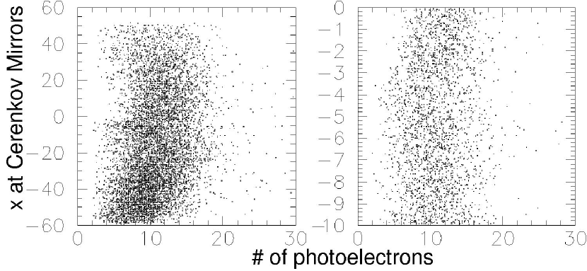
Figure 3.6: HMS Čerenkov signal versus horizontal position at the mirrors. On the right is a blowup of the overlap region. Note that even at the lowest point in the dip, the mean signal is still 8-9 photoelectrons.

In the SOS, the mean signal is $\sim$12 photoelectrons, and the hardware threshold in the trigger corresponds to 1.7 photoelectrons. In the final analysis, a signal of 3.3 photoelectrons is required, giving an efficiency of 99.8%. There is less material in front of the SOS Čerenkov tank, and therefore the pion rejection limit caused by knock-on electrons is $\sim$900:1. However, in the SOS, the ADC signal had significant noise, and the Čerenkov signal would occasionally exceed the initial 2 photoelectron cut. Because of this, the cut was raised to 3.3 photoelectrons, reducing the probability that the noise will cause a pion to exceed the cut to $\leq 0.5$%. This means that the online cut rejects pions at $\sim$160:1, after taking into account the pions which produce knock-on electrons and the pions which have significant noise in the ADC. However, the cut could not be increased above 3.3 photoelectrons without causing a significant inefficiency for electrons, due to the variation of the signal near the edges of the mirrors.

While the average signal is $\sim$12 photoelectrons, it is reduced in the regions where the mirrors overlap due to imperfections in the mirrors and possible misalignment. Therefore, the 3.3 photoelectron cut had a significant inefficiency in some regions. Figure 3.7 shows the SOS Čerenkov signal as a function of vertical position at the mirrors. There is a clear reduction in the signal in the region of overlap of the mirrors (shown in greater detail in the figure on the right). In this overlap region, the Čerenkov has a significant inefficiency for a 3.3 p.e. cut, but lowering the cut would reduce the pion rejection to unacceptable levels. However, in the final analysis the data is binned in the Nachtmann variable $\xi=2x/(1+\sqrt{1+\frac{4M^{2}x^{2}}{Q^{2}}})$ (see section 3.3.9), and while the inefficiency for a 3.3 photoelectron cut is large ($\sim 5$%) where the signal is the lowest, the inefficiency in any $\xi$ bin is much smaller ($\leq 2\%$). Figure 3.8 shows the same data as figure 3.7, but now as a function of $\xi$. The gap that is well localized in $x_{cer}$ is now almost evenly spread out over the lower half of the $\xi$ acceptance. Because the data is binned in $\xi$ for the extraction of the cross section (see section 3.3.9), the worst-case inefficiency for a 3.3 photoelectron cut is only 1-2%. We normalize the data for the average inefficiency (1%), and assign an uncertainty of 1% to cover the variation of the efficiency over the $\xi$ bins.

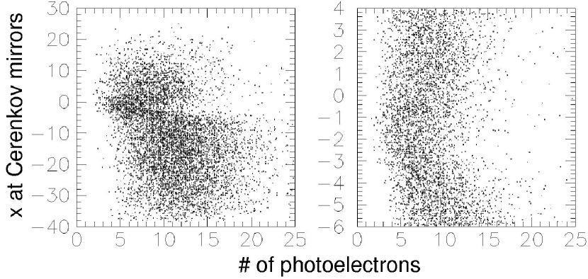
Figure 3.7: SOS Čerenkov signal versus horizontal position at the mirrors. On the right is a blowup of the overlap region. Note that even at the lowest point in the dip, the mean signal is still 8-9 photoelectrons.

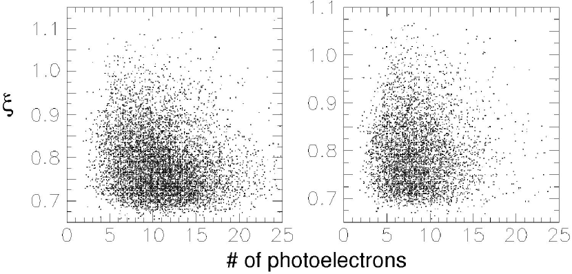
Figure 3.8: SOS Čerenkov signal versus $\xi$. While there is a significant localized reduction of the signal at the overlap of the mirrors, the loss of signal is spread out nearly uniformly over the lower half of the $\xi$ acceptance of the spectrometer. The figure on the right shows the signal versus $\xi$ for data near the overlap regions (same cut as in figure 3.7.

The lead-glass shower counter was also used to reduce the pion contamination. Because the calorimeter does not cover the complete acceptance of the spectrometer (some tracks miss the calorimeter for extreme values of $\delta$), the reconstructed focal plane track was projected to the calorimeter and a fiducial cut was applied requiring that the track was at least 3 cm inside of the edge of the calorimeter.

In the HMS, the intrinsic calorimeter energy resolution is $\sim$6%$/\sqrt{E}$, but during the first half of the running, the ADC pedestals had small fluctuations, and the overall resolution was somewhat worse. Figure 3.9 shows the calorimeter energy as a function of time for a run where there pedestal values varied during the run. The ADC offsets make discrete jumps, leading to offsets in the measured energy for pions and electrons. In cases like figure 3.9, the separation between the pions and electrons (pions should appear at $\sim$0.3 GeV) is large enough that the pion rejection is unaffected. In addition, because the calorimeter energy fraction cut was lowered as the momentum increased (see below), the calorimeter cut is efficient enough that there is no significant inefficiency for electron detection for this run. The fluctuations only occured during the first half of the run (after which the bad ADC was replaced), and only affected $\sim$1/3 of the runs during that period. For the majority of the runs, the electron energies were large and the fluctuations were small. For these cases, the pion rejection and electron efficiency were not significantly affected. For runs where the electron energies were smaller or the fluctuations large, the energy cut was lowered if the Čerenkov cut and reduced pion rejection were sufficient to remove the pions. Runs where this was not possible due to the large pion background were removed from the data set. For some of these runs it would have been possible to measure the pedestal shifts using the values from blocks that had no signal from the electron. However, all of the data that was rejected was taken at kinematics where there were other runs which were unaffected by the pedestal jumps. Therefore it was decided to eliminate the bad runs entirely and take the reduced statistics, rather than trying to correct these runs and have larger systematic uncertainties due to reduced electron efficiency or a non-negligible pion background.

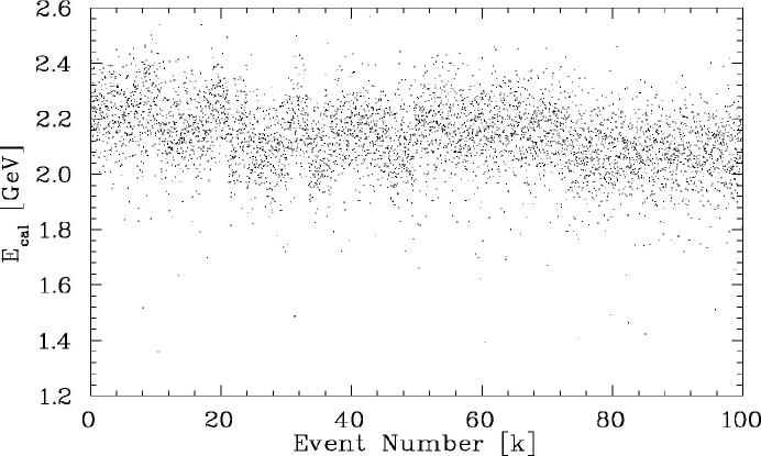
Figure 3.9: HMS calorimeter energy versus time for one of the runs with fluctuating ADC pedestals. The HMS was set at 2.2 GeV/c, so electrons deposit 2.2 GeV and pions deposit $\sim$0.3 GeV in the calorimeter.

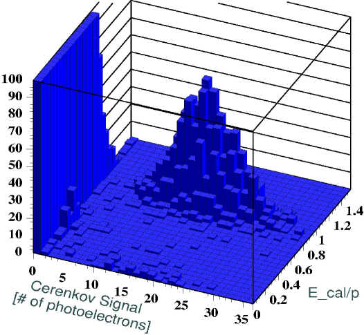
Figure 3.10: Calorimeter ($E_{cal}/p$) versus Čerenkov for HMS run with a pion to electron ratio of approximately 70:1. The majority of the pions occur at 0 photoelectrons, though approximately 1% have a single photoelectron signal from noise.

The HMS detected particles with momenta between 0.995 GeV/c and 4 GeV/c. For the lowest momentum, where the resolution is the worst and the pion-electron separation is the smallest, the electron was required to have an energy fraction, $E_{cal}/p$, greater than 0.7. This cut is always $3\sigma$ or greater, ($\mathrel{\raise 1.29167pt\hbox{$>$}\mkern-14.0mu\lower 2.58334pt\hbox{$\sim$}}99.9\%$ efficient) even for runs where the resolution is worse than usual due to pedestal drift. As the momentum increases, the energy fraction measured for electrons is still one, and the pion peak shifts to lower energy fraction ($\sim 0.3$ GeV/$p$). During a portion of the running, all at higher momenta, the calorimeter ADC signals made discrete jumps during the course of a run. Therefore, while the resolution of the electron peak improves as the energy increases, there were some runs where the effective width was significantly larger then the normal $6\%/\sqrt{E}$. Therefore, the energy fraction cut was varied with energy, so that it was always highly efficient ($>99.8\%$) for all energies, including runs where the pedestals varied during the run. The final cut used was:

$$E_{cal}/p>0.7-0.07*(p-0.995)$$ (3.3)

which corresponds to an energy cut of $0.7315p-0.07p^{2}$. As the momentum increases, the energy resolution improves and the energy fraction cut decreases, increasing the electron efficiency of the cut. In addition, the absolute energy cut increases with momentum (for momentum values below 5 GeV/c), while the energy of the main pion signal remains constant. Therefore, the pion rejection is also improved as the momentum increases. However, even at very high energies there is still a small probability that a pion will deposit enough energy and be misidentified as an electron. While the majority of pions deposit roughly 0.3 GeV in the calorimeter, there is a small tail in the calorimeter energy distribution for pions that extends out to the full pion energy. The tail comes from pions which undergo a charge exchange interactions and become neutral pions. The neutral pions can decay into photons in the calorimeter, and their full energy can be deposited in the calorimeter. For the kinematics measured in e89-008, it is the lower momentum values where the pion rejection is most important, and in this region it is the resolution of the pion energy deposition that limits the pion rejection, rather than the tail. The HMS calorimeter pion rejection is $\sim$ 25:1 at 1 GeV, 50:1 at 1.3 GeV, and 150:1 at 1.5 GeV. For the HMS, the combination of Čerenkov and Calorimeter cuts reduces the pion contamination in the final data to $<1.0\%$ for all kinematics. Figure 3.10 shows calorimeter signal ($E_{cal}/p$) versus the Čerenkov for the HMS at a central momentum of 1.11 GeV/c, with a pion to electron ratio of $\sim$70:1. For some higher momentum runs, the ratio of pions to electrons is much higher, but the calorimeter pion rejection improves as the energy increases, making this one of the worst cases for pion contamination. Figure 3.11 shows the pion to electron ratio (as calculated from the hardware scalers) versus the momentum for all of the data runs. The line shows the $\pi$/e ratio at which there is a 1% contamination after the particle identification cuts. The $\pi/e$ ratio for the run is determined by taking the ratio of the PION and ELLO hardware scalers. At very high $\pi/e$ ratios, the ELLO scaler will have a significant contribution from pions which produce a knock-on electron of sufficient energy to give a signal in the Čerenkov. The ELLO scaler was corrected for the expected pion contamination, based on the pion rejection of the Čerenkov trigger signal. Therefore, the calculated $\pi$/e ratio is accurate for $\pi$/e $\geq$ one. However, for $\pi$/e $\ll 1$, the calculated $\pi$/e is too high, due to electrons which do not fire the Čerenkov discriminator and are identified as pions.

Figure 3.11: Ratio of pions to electrons in the HMS as a function of momentum. The $\pi$/e ratio is calculated from the hardware scalers, and corrects for pion misidentification in the scaler signals. The line shows the $\pi$/e ratio where there is a 1% pion contamination after the particle identification cuts.

For the SOS, the calorimeter is physically identical to the HMS except for the total size. The performance of the SOS calorimeter was nearly identical to the HMS, except that it did not have problems with drifts in the ADC pedestals. The resolution for the SOS calorimeter was $\mathrel{\raise 1.29167pt\hbox{$<$}\mkern-14.0mu\lower 2.58334pt\hbox{$\sim$}}6\%/\sqrt{E}$. However, because the SOS was operated at lower momenta than the HMS, the cut had to be tighter than in the HMS. For the SOS, the energy fraction had to be greater then 0.75. For the lowest SOS momentum, p=0.74 GeV, the energy resolution is $\sim$7%, and the cut is $\mathrel{\raise 1.29167pt\hbox{$>$}\mkern-14.0mu\lower 2.58334pt\hbox{$\sim$}}$99.8% efficient. The pion rejection factor is given as a function of momentum in table 3.2. Figure 3.12 shows the pion to electron ratio (as calculated from the hardware scalers) versus the momentum for all of the data runs. The lines show the $\pi$/e ratio at which there is a 1% (5%) contamination after the particle identification cuts. The hardware scalers are corrected in the same way as in figure 3.11, so the $\pi$/e ratio shown is accurate for $\pi$/e$>1$, but not for small values. The pion rejection of the cut is measured very accurately at 1.11 GeV/c, where there were high statistics runs taken without the particle identification trigger. For the lower momentum runs, the pion rejection shown is determined by assuming that the pions have the same energy distribution at the lower momenta, and reducing the energy cut to 0.75 times the central momentum, which is the cut used in the data analysis (E/p=0.75). However, this underestimates the pion rejection because it assumes that the tail of the pion distribution goes up to 1.11 GeV, when in fact it must fall to zero above the actual pion momentum. A small correction was applied to remove the part of the energy distribution above the pion momentum, but this only removes the end of the pion energy tail, it does not reduce it at intermediate energies. Thus, the pion rejection assumed in figure 3.12 is a lower limit.

Eπ	Pion Rejection
0.75 GeV	10:1
0.90 GeV	20:1
1.11 GeV	50:1
1.30 GeV	150:1

Table 3.2: SOS calorimeter pion rejection as a function of pion energy.

Figure 3.12: Ratio of pions to electrons in the SOS as a function of momentum. The $\pi$/e ratio is calculated from the hardware scalers, and corrects for pion misidentification in the scaler signals. The solid line shows the $\pi$/e ratio where there is a 1% pion contamination after the particle identification cuts, and the dashed line shows the 5% contamination level. The pion rejection is measured very accurately at 1.11 GeV/c, but the pion rejection at lower momentum values is a lower limit of the pion rejection achieved. Therefore, the final pion contamination is always below the 3% worst-case shown here.

For some runs at 74^∘ (and momentum below 1 GeV/c), there is a non-negligible pion contamination after the shower counter and Čerenkov cuts are applied. The worst case pion contamination is below 3%. However, for the large angle data we subtract the charge-symmetric electron background (see section 3.3.4) by subtracting positive polarity data taken at identical kinematics. If the production cross sections for $\pi^{+}$ and $\pi^{-}$ are identical, then the pions remaining after cuts in the electron running will be subtracted out by pions in the positive polarity running. However, there are two errors associated with this subtraction. As discussed in section 3.3.4, the positive polarity runs are only taken for some of the targets. The background for the other targets is scaled according to the effective thickness of the target. Because the pion and positron production rates may have a different dependence on target thickness, the normalization used in subtracting out the positrons is not exactly correct for the pions. In addition, if the production rates for positive and negative pions differ, then the subtraction will be incorrect. The positive polarity measurements are taken with the thick targets, and so the only uncertainty in the subtraction of the pions is the ratio of $\pi^{+}$ to $\pi^{-}$. As long as the $\pi^{+}$ cross section is not more than twice the $\pi^{-}$ cross section, the worst case error in the cross section will still be 3% (a 3% $\pi^{-}$ contamination if the $\pi^{+}$ cross section is zero, or a 3% over-subtraction of the pions if the $\pi^{+}$ cross section is twice the $\pi^{-}$. For the thin targets, there is an additional uncertainty due to the extrapolation from the measured thick target backgrounds to the thin targets. However, for the thin target data, the pion contamination is lower than for the thick target data. Therefore, the worst case pion contamination before subtraction is $<$1.5% for the thin target data, and the maximum final error is still 3%, even if the the number of $\pi^{+}$ subtracted is three times the number of $\pi^{-}$ present, due to the difference in $\pi^{+}$ and $\pi^{-}$ cross section, and the error made in the extrapolation to thin targets. We assume a full pion subtraction for the cross section, and apply no normalization, and assume an uncertainty of 100% in the subtraction of $\pm$70% of the expected pion contamination, leading to a maximum uncertainty of $\pm$3%. Because of the uncertainties caused by the large charge-symmetric background subtraction, and the low statistics for the 74^∘ running, the uncertainty from the possible pion contamination is not a large contribution to the final uncertainty. We assign a 3% uncertainty to the low momentum SOS data due to uncertainty in the pion rejection/subtraction.

3.3.4 Background Rejection

In addition to rejecting pions, it is also necessary to reject background electrons. These are electrons that are not coming from the scattering of beam electrons in the target. There are two main sources of background electrons. First, there are events where particles coming from upstream or downstream of the target (beam halo scattering off of the beam pipe or background from the beam dump) enter the spectrometer after the magnets and create low energy electrons that reach the detectors. There are also ‘secondary’ high energy electrons that are produced in the target rather than being scattered from the beam.

In the HMS, background events come from low energy electrons from the beam dump scattering into the detector hut near the exit of the dipole. There is a vacuum pipe that runs through the magnets and into the detector hut. Particles in the hall that pass through the vacuum pipe after the magnets can be scattered into the detector hut (or produce knock-on electrons that make it into the hut). When the focal plane tracks are projected backwards to a point just before the entrance to the shielding hut, the events that come from scattering in the vacuum pipe can be seen as a ’ring’ in the $x$-$y$ plane, while real events are seen in the center. Prior to the experiment, shielding was added to decrease the background from particles entering the spectrometer after the magnets. In the analysis, a cut is applied to remove events that come from outside of the vacuum pipe. In addition, because these are low energy electrons, most are rejected in the calorimeter cut. The combination of the cut at the entrance to the hut and the calorimeter is sufficient to eliminate this source of background. Figure 3.13 shows a run with a very low rate of real events as well as a high rate run. In the low rate run, the events coming from the vacuum pipe are clearly visible. Because most of the background particles in the hall come from the beamline or the beam dump, they are traveling nearly horizontally when they pass through the vacuum pipe. This means that they pass through significantly more material if they strike the top or bottom of the pipe, and so have a greater chance of being scattered into the hut than particles which pass through the sides of the pipe.

There were also a significant number of events in which particles above the spectrometer momentum would hit the bottom of the dipole and be scattered into the spectrometer, or produce lower energy electrons which made it through the last part of the dipole and into the hut. Before e89-008, shielding was added at the back of the dipole, in between the vacuum pipe and the magnet in order to reduce the background. In the analysis, the combination of the calorimeter cut, the cut at the hut entrance, and the cuts on reconstructed target quantities eliminated these events.

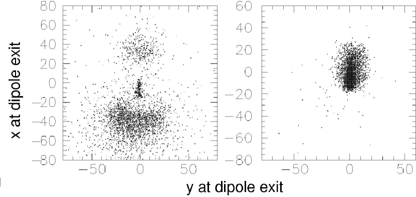
Figure 3.13: Background events coming from the dipole exit can and vacuum pipe. The data on the left come from a run with a very low rate of real events. The run on the right is a run with a high rate of real events. The figures show $x$ versus $y$ 750 cm in front of the focal plane (near the exit of the dipole) before tracking or calorimeter cuts have been applied. Note that $-x$ corresponds to the top of the dipole can.

In the SOS, the back portion of the second dipole is inside of the shielding hut. Therefore, low energy electrons entering the vacuum line outside of the hut would be swept away by the dipole and not reach the detectors. In the SOS, there is no way for a particle to reach the vacuum pipe without passing through the magnets or penetrating the shielding hut. There are two small gaps in the shielding where the SOS dipole enters the hut. This allows events to enter the hut without passing through the magnets, but these events are easy to reconstruct back to the hole. Figure 3.14 shows $x$ versus $y$ at the entrance to the shielding hut. At $x\sim-29$ cm, there are events that come through gaps in the shielding where the dipole enters the hut. While the majority of events coming through the gaps are rejected in the tracking cuts, the events shown have passed the $\delta$, $\theta$, and particle identification cuts. In order to remove these events, we project the track to the wall of the shielding hut, and require $(x_{fp}-100x^{\prime}_{fp})>-24$ cm.

Figure 3.14: $y_{fp}$ versus $x_{fp}$ projected back to the front of the SOS shielding hut, after tracking and particle identification cuts have been applied. At $x\sim-28cm$, there are events coming through gaps in the shielding where the dipole enters the detector hut. Many of the events have been rejected by the $\delta$ and $\theta$ cuts, but some still pass those cuts. A cut has been applied at $x_{dipole}$ = -24 cm.

In addition to background coming from the low energy electrons, there are secondary electrons produced in the target. Since they are secondary electrons, rather than scattered electrons, they are a background for the measurement. The main background of secondary electrons most likely comes from electro-production and photo-production of neutral pions. These pions then decay into photons which can produce positron-electron pairs. This background is charge-symmetric, and can be measured by running with the spectrometers in positive polarity, and detecting the produced positrons. For the largest angles (55^∘ and 74^∘), this background was significant. In this case, the positron production cross section was fit from our measurements and subtracted from the electron data. For the smaller angles, this background was negligible ($<$1%).

Positive polarity data was typically only taken for one or two targets for each kinematics. We parameterize the ratio of positron to electron production in terms of the target thickness (in radiation lengths), and extrapolate the measured positron cross sections to the thickness of the other targets. The $e^{+}/e^{-}$ ratio can vary by up to a factor of four between the different targets, but the positron rate differs from the parameterization by only $\sim$10% over this range. Most of the positive polarity data were taken with the thick targets in order to maximize the positron statistics. Therefore, the extrapolation of the measured $e^{+}/e^{-}$ ratio between the different thick target had only a small uncertainty $\approx$1-2%, while the extrapolation to thin targets was uncertain at the $\sim$10% level. However, the ratio of positrons to electrons was near unity for the thick targets, but only $\sim$30% for the thin targets. Therefore, the uncertainty due to the target thickness extrapolation is $\mathrel{\raise 1.29167pt\hbox{$<$}\mkern-14.0mu\lower 2.58334pt\hbox{$\sim$}}$3% of the total electron cross section. Rather than making a point by point subtraction of the measured positron cross section, all positron data at 55^∘ and 74^∘ was fit in order to obtain the cross section to be subtracted due to the charge-symmetric background. The uncertainty in the positron fit was a combination of the uncertainty due to target thickness differences, and due to the statistics of the measurements.

Figure 3.15 shows the background subtracted electron and raw positron cross sections for scattering from the thick Gold at $55^{\circ}$, and from the thick Iron and thin Carbon targets at $74^{\circ}$. At $55^{\circ}$, the charge symmetric background is $\sim$10% of the electron cross section for the thick targets, and $\sim$3-4% for the thin targets. At $74^{\circ}$, the background can be equal to or larger the electron cross section for the thick targets, and $\sim$20% for the thin targets.

Figure 3.15: Electron and positron cross sections. The filled diamonds are the measured electron cross section after subtraction of the charge symmetric background. The hollow diamonds are the measured positron production cross section. The top plot is 55^∘ data measured with the thick Gold target (5.8% of a radiation length), the middle is 74^∘ with the thick Iron target (5.8% r.l.), and the bottom is 74^∘ data with the thin Carbon target (2.1% r.l.). The solid line is the fit to all positron data that is subtracted from the electron cross section.

3.3.5 Electronic and Computer Deadtime.

The main corrections to the measured number of counts come from data acquisition dead times and inefficiencies in the trigger hardware and the drift chambers. Electronic deadtime is caused when triggers are missed because the hardware is busy when an event that should generate a trigger comes in. When a logic gate in the trigger is activated, the output signal stays high for a fixed time. If another event tries to activate the gate in that time, it is ignored. If the mean event rate is $R$, then the probability of finding $n$ counts in a time $t$ is given by the Poisson distribution:

$$P(n)=\frac{(Rt)^{n}e^{-Rt}}{n!},$$ (3.4)

and the probability distribution for the time between events is

$$P(t)=Re^{-Rt}.$$ (3.5)

An event will be missed if it comes within a time $\tau$ of an event accepted by the gate, where $\tau$ is the gate width of the logic signal. If the probability for this to occur is small enough, then this is nearly identical to the probability of an event coming within time $\tau$ of the previous event (whether or not the previous event triggered the logic gate). Therefore, for small dead times the fraction of measured events is equal to the probability that the time between events will be greater than $\tau$:

$$\frac{N_{measured}}{N_{total}}=\int_{\tau}^{\infty}Re^{-Rt}dt=e^{-R\tau}.$$ (3.6)

In the trigger, all of the logic gates have a width of 30 ns, except for the hodoscope discriminators. The hodoscope discriminators have a very low threshold, and so their gate width was set to 50 ns in order to eliminate double pulsing of the discriminators caused by ringing of the signal. However, the hodoscope discriminators are not dead when their outputs are active. If a new signal comes in while the discriminator output is high, the output signal is extended to 60ns after the latest hit. Therefore, $\tau=30$ns for the electronic dead time. For the trigger rates measured in this experiment, the live time was very close to 100%, and could be approximated by $e^{-R\tau}\approx 1-R\tau$. To correct for the dead time, we generated four versions of the final electron trigger, each with a different gate width ($\tau$ = 30,60,90, and 120 ns). We then made a linear extrapolation to zero dead time in order to determine how many events were lost in the real electron trigger ($\tau$ = 30 ns). For each run we measured the electronic dead time and corrected the final cross section for the number of triggers lost. For the HMS, the maximum correction was $\approx$ 0.1%, and for the SOS it was $\mathrel{\raise 1.29167pt\hbox{$<$}\mkern-14.0mu\lower 2.58334pt\hbox{$\sim$}}$ 0.02%.

There is another source of electronic deadtime, coming from singles triggers which were generated properly, but which were interpreted as coincidence triggers due to a random coincidence with an SOS trigger. As described in section 2.7, the trigger included HMS and SOS singles triggers, as well as coincidence triggers. Coincidence triggers only came as the result of random electron coincidences in the spectrometers. While the COIN triggers formed in the 8LM (see figure B.1) were prescaled away at the trigger supervisor (TS), if the HMS and SOS singles triggers come within the latching time of the TS ($\sim$7 ns), then the event will be treated as a coincidence. While each coincidence trigger indicates a trigger for both the HMS and SOS, they are not analyzed because the timing was not set up properly for coincidences, and there could be mistiming in the ADC gates and TDC stops. Because an event with HMS and SOS events coming within the TS latching time will be treated as a coincidence event, an SOS trigger coming between 7 ns before and 7 ns after an HMS trigger will cause the event to be tagged as a coincidence. If the rate of triggers in the SOS is $R$, and the time window for a coincidence trigger is $\tau$ (15 ns in this case), then the probability of an SOS trigger causing a random coincidence with an HMS trigger is:

$$\int_{0}^{\tau}Re^{-Rt}dt=1-e^{-R\tau}.$$ (3.7)

For $R\tau\ll 1$, the coincidence blocking deadtime can be approximated as $1-e^{-R\tau}\approx 1-(1-R\tau)=R\tau$. For the most part, the coincidence blocking caused an inefficiency between $10^{-7}$ and $10^{-4}$ of the events. However, there were a few runs where the SOS singles rate was high enough to cause $\mathrel{\raise 1.29167pt\hbox{$>$}\mkern-14.0mu\lower 2.58334pt\hbox{$\sim$}}$0.2% of the HMS events to be taken as coincidence triggers. However, for all of the runs where the SOS rate was high enough to cause a noticeable dead time, the SOS triggers were prescaled by a factor of 100 or more. This reduced the number of SOS triggers available to make a false coincidence with the HMS in the TS, and made the dead time negligible for these runs as well.

A more significant source of dead time for this experiment was the computer dead time. In this case, events are lost because a hardware trigger is formed when the data acquisition system is busy processing the previous event. The total processing time for an event is $\sim$300-400$\mu$s. However, when running in buffered mode the data acquisition can accept a new trigger before the old trigger is fully processed. It is only dead for $\sim$100$\mu$s, while the fastbus conversion of the data is in progress (see section 2.7.5 for more details). The computer dead time is measured by counting the number of triggers that were formed and the number of triggers that were processed by the Trigger Supervisor. The number processed over the number generated is the live time of the data acquisition system. The dead time is calculated for each run, and the cross section is corrected for the lost triggers. Figure 3.16 shows the computer deadtime for all runs. A few runs were taken in non-buffered mode, and have a processing time of 300-400$\mu$s, depending on the average size of the event. The average event size is dependent on the ratio of HMS to SOS events and the pion to electron ratio, since electrons will usually have extra ADC and TDC values for the calorimeter and Čerenkov signals. For some early runs, the parallel readout of multiple crates was not enabled and the event processing time was roughly 800$\mu$s. Note that at very high rates ($\mathrel{\raise 1.29167pt\hbox{$>$}\mkern-14.0mu\lower 2.58334pt\hbox{$\sim$}}$2kHz) the deadtime is larger than expected for a 100$\mu$s processing time. This is because the minimum time between events is 100$\mu$s in buffered mode, but each event still requires $\sim$400 $\mu$s to process fully. Therefore, the maximum rate is $\sim$2500 Hz, and the effective processing time increases from 100 to 400$\mu$s as the incoming event rate goes beyond 2500Hz.

Figure 3.16: Measured computer dead time vs. pretrigger rate. The solid line is the expected value for a processing time, $\tau$, of 100$\mu$s, the dashed line is for $\tau$=350$\mu$s and the dotted line is $\tau$=800$\mu$s. Note that there is some uncertainty in the calculated pretrigger rate. The value plotted is the average rate over the entire run. Therefore, if the beam is off for part of the run, or if the current changes as a function of time, the pretrigger rate shown will not exactly represent the instantaneous rate that determines the deadtime.

3.3.6 Trigger Efficiency.

Events are also lost due to detector inefficiencies that cause triggers to be missed, or inefficiency in the drift chambers or tracking algorithm that cause real events to be lost in the event reconstruction. Inefficiencies in the hodoscopes can cause a plane not to fire. The efficiency of each scintillator is determined by taking tracks that point to the center of the paddle (excluding the outer 2 cm of each paddle in the HMS, 1.25 cm in the SOS) and determining how often each paddle fires. Using the measured efficiency of the scintillators, we calculate the probability of missing a trigger due to hodoscope inefficiency and correct the counts for this loss. Because the trigger requires only three of the four planes, the scintillator trigger efficiency is always high, $>$99.4% for all HMS runs and $\mathrel{\raise 1.29167pt\hbox{$>$}\mkern-14.0mu\lower 2.58334pt\hbox{$\sim$}}$99.8% for the SOS. In the HMS, the data is corrected run by run for the scintillator inefficiency, as determined by the measured hodoscope efficiencies for the run, and a 0.05% systematic uncertainty is assumed in the correction.

In the SOS, the calculated hodoscope efficiency is too low, because multiple scattering in the detector makes it hard to determine the efficiency for the rear hodoscopes using tracking information (see appendix A for details on the efficiency calculations). The calculated efficiency for S1X is always better than 99.90%, and for S1Y, it it always better than 99.93%. The calculated efficiency for the rear planes is only about 90%, and shows a small momentum dependence. This is because the efficiency is calculated by taking events where the track points within 1 cm of the center of a hodoscope element, and looking to see if that hodoscope had a signal. In the SOS, the multiple scattering causes some of these events to miss the identified hodoscope element (In the HMS, the hodoscope paddles are wider, and the the multiple scattering is smaller because of the higher momentum). This means that the tracking based efficiency measurements cannot be used to determine the overall hodoscope efficiency. However, for running at a fixed momentum, the measured tracking efficiencies were extremely stable ($\mathrel{\raise 1.29167pt\hbox{$<$}\mkern-14.0mu\lower 2.58334pt\hbox{$\sim$}}$0.2%) over time, indicating that there was never any significant loss of efficiency during the run. The hodoscope efficiency is also measured by looking at the fraction of triggers for which the plane had a hit. While this does not measure the efficiency, it is a fairly good measure of the overall efficiency of the plane. From this efficiency, the front and rear $y$ planes have nearly identical efficiencies, and the front $x$ plane has a slightly smaller efficiency than the rear $x$ plane (due to events which enter at the bottom of the detector stack and pass below the front drift chamber and S1X hodoscope plane. This indicates that the true hodoscope efficiency for the rear planes is comparable to the front planes. Based on the track-independent measurement of the efficiency, and the stability of the track-dependent efficiency, we assume that the rear hodoscopes were at least 98% efficient, giving a 3/4 trigger efficiency of $>$99.95%. Therefore, for the SOS we do not apply a correction for the hodoscope trigger efficiency, and apply a 0.01% systematic uncertainty.

Additional trigger inefficiency can come if the particle identification signals in the trigger do not fire. The thresholds in the trigger are $\mathrel{\raise 1.29167pt\hbox{$>$}\mkern-14.0mu\lower 2.58334pt\hbox{$\sim$}}$99.5% efficient for the Čerenkov, and $>$90% efficient for the Calorimeter (better than $99\%$ efficient for higher energies). Since the trigger requires only one of the calorimeter signal or the Čerenkov signal, the PID is greater than 99.95% efficient in the trigger. Because the PID cuts in the analysis are tighter than the cuts in the trigger, we do not apply a correction for inefficiency in the trigger PID, we apply a single correction to take into account the total inefficiency of all PID cuts. The electron efficiency and pion rejection of the cuts was determined by taking runs with the particle identification signals removed from the trigger. In addition, the pion rejection is checked for each run by examining the calorimeter energy distribution after the final Čerenkov cut has been applied to insure that there is a clean separation of the pion and electron peaks, and that the pion contamination is at or below the level expected from the Čerenkov and calorimeter pion rejection.

3.3.7 Tracking Efficiency.

Even if a trigger is formed, there will be some events where there is not enough information to reconstruct a track. The main sources of inefficiency of this kind are events where too many or too few wires fire in the drift chambers. If too few wires fire, the left-right ambiguity cannot be well determined, and a track is not fit. If too many wires fire, then the tracking takes a large amount of CPU time (finding all pairs and combinations of pairs of hits), and the chance of having a ‘noise’ hit included in the track increases.

The tracking efficiency is defined as the number of events for which a track is found, divided by the number of ‘good’ events (i.e. the number which we expect to have a real track). A trigger is defined as being a ‘good’ event if there was a trigger for the spectrometer, the time of flight determined before tracking determines it was a forward-going particle (rather than a cosmic ray), and one of the two drift chambers had less than 15 hits. We assume that events where both chambers have more than 15 hits are caused by electrons (or pions) which scrape the edge of one of the magnets and cause a shower of particles. Therefore, while there was a real particle, it was not within the acceptance of the spectrometer, and we should not correct for losing it due to tracking inefficiency. An event in which only one drift chamber had 15 hits is assumed to be a good event with additional hits due to noise in the chamber (which sometimes causes all 16 wires on a single discriminator card to fire) or the production of a knock-on electron which produces another short track and therefore another cluster of hits in one of the chambers. Since both of these conditions occur for good events within the acceptance of the spectrometer, we correct for these losses in the tracking efficiency. Once we require that one chamber was clean ($<$15 hits), then the number of tracks is corrected for the fraction lost to a single noisy chamber, a chamber with less than 5 planes hit, or events in which a consistent track cannot be made from the hits in the two chambers (see sections 3.1.1 and A.3.3 for details on the tracking algorithm).

The tracking efficiency is calculated for all events, events passing a particle identification cut, events within a fiducial region of the hodoscopes, and events passing both the fiducial and PID cuts. This is because the efficiency calculated for all events includes the tracking efficiency for pions and background events as well as the real electrons. For runs where the electron cross section is low, the majority of events are pions or background electrons. By applying a PID cut, we reject the majority of the pions. By applying the fiducial cut, we look at the central and low momentum region, where the electron cross section is largest, and the signal to background ratio is larger. The data is corrected for the efficiency calculated using events passing the PID and fiducial cuts.

Figure 3.17: HMS Tracking efficiency as a function of time.

The HMS tracking efficiency is typically 93-97%. Roughly 1% of the loss comes from the drift chamber inefficiency causing too few hits, and the rest comes primarily from noise in a single chamber giving more than 15 hits in a plane. Figure 3.17 shows the HMS tracking efficiency as a function of time. The tracking efficiency has large variations, but it was checked for several low and high tracking efficiency runs that the majority of event lost came from random noise in the amplifier/discriminator cards or the TDC. For the SOS, the tracking efficiency is typically between 95.5% and 96.5%. Roughly 1% comes from drift chamber inefficiency, and the rest comes from noisy amplifier/discriminator cards. Figure 3.18 shows the SOS tracking efficiency as a function of time. The chamber noise in the SOS is significantly more stable than in the HMS.

Figure 3.18: SOS Tracking efficiency as a function of time.

The main uncertainty in this correction comes from the assumption that all events with one noisy chamber correspond to real events, and events with two noisy chambers correspond to bad (scraping) events. By looking at patterns of drift chamber and hodoscope hits for events where both chambers have $>$15 hits, we determined that $\geq$90% of these events come from showers in the detector. Since the maximum fraction of these events is $<$5% of the total events (after the PID and fiducial cuts), the maximum loss of good events is $\mathrel{\raise 1.29167pt\hbox{$<$}\mkern-14.0mu\lower 2.58334pt\hbox{$\sim$}}$0.5%. Similarly, $\geq$90% of the events where one chamber has $>$15 hits correspond to events where there is a single good track in the chambers and hodoscopes, but additional hits in one chamber, usually for a set of wires on a single amplifier/discriminator card. Usually 3-4% of the events have one noisy chamber, leading to a typical correction for ‘junk’ events of $\leq$0.4%. For a handful of runs, the number of events lost due to one chamber with $>$15 hits was as high as 8%, leading to a possible error of $\leq$0.8%. We correct the data for the measured efficiency (after PID and fiducial cuts) and assign an uncertainty of $\pm$0.5% to the correction.

3.3.8 Spectrometer Acceptance

For a fixed angle and momentum setting, the HMS (and SOS) will measure data in a limited range of angles and momenta around the central values. As we move away from the central kinematics, some fraction of the events will be lost if they hit the collimator, scrape the walls of the magnets, or miss detector elements required for the trigger or in the data analysis. For scattering with a cross section $\sigma$, the number of events detected in the spectrometer will be a function of the point where the scattering occurs in the target, and the kinematics of the spectrometer:

$$N=\int d\delta dx^{\prime}dy^{\prime}dxdydz\cdot\sigma(\delta,x^{\prime},y^{\prime},x,y,z)\cdot A^{6}(\delta,x^{\prime},y^{\prime},x,y,z),$$ (3.8)

where $A^{6}(\delta,x^{\prime},y^{\prime},x,y,z)$ is the acceptance function of the spectrometer which represents the probability that a scattering event coming from the point $(x,y,z)$, with kinematics defined by $\delta,x^{\prime},$ and $y^{\prime}$ will be detected. We can use a model of the spectrometer to perform a Monte Carlo calculation of the acceptance function of the spectrometer. However, it is not feasible to generate enough statistics in the Monte Carlo to have a high precision calculation of acceptance as a function of all 6 variables. Therefore, we would like to define a simplified acceptance function, which averages over the behavior of several of the variables.

As long as the target is thin enough that there is no significant loss of beam intensity as a function of position along the target, the cross section is independent of $x,y,$ and $z$. The cross section is then just a function of $\delta$, $x^{\prime}$, and $y^{\prime}$. This means that we can now integrate over $x,y$, and $z$ over the region of interest (as defined by the position and size of the beam and target), and come up with an acceptance function in terms of just $\delta$, $x^{\prime}$, and $y^{\prime}$ which takes into account the acceptance of the spectrometer in $x,y,z,$ and which is independent of the scattering kinematics:

$$N=\int d\delta dx^{\prime}dy^{\prime}\cdot\sigma(\delta,x^{\prime},y^{\prime})\int dxdydz\cdot A^{6}\equiv\int d\delta dx^{\prime}dy^{\prime}\cdot\sigma(\delta,x^{\prime},y^{\prime})\cdot A^{3}(\delta,x^{\prime},y^{\prime}).$$ (3.9)

In order to further simplify the acceptance function, we can fix the central angle of the spectrometer, and convert from $x^{\prime}$ and $y^{\prime}$ to the in-plane and out-of-plane scattering angles $\theta$ and $\phi$. Because the inclusive cross section is independent of $\phi$, we can integrate over $\phi$ and define a two-variable acceptance function, $A^{2}(\delta,\theta)=\int A^{3}(\delta,\theta,\phi)d\phi$, such that

$$N=\int d\delta d\theta\cdot\sigma(\delta,\theta)\cdot A^{2}(\delta,\theta).$$ (3.10)

We can generate events in $x,y,z,\delta,\theta,$ and $\phi$ in the Monte Carlo, and bin the results as a function of just $\delta$ and $\theta$ in order to determine the acceptance of the spectrometer. The Monte Carlo model has three main elements: the event generator, the transportation of the particle through the magnets, and the list of materials and apertures that cause multiple scattering or stop the particles. The event generator creates a large set of initial particles distributed uniformly in $\delta$, $\theta$, $\phi$, $x$, $y$, and $z$. The particles are then run forward through the model of the spectrometer, and focal plane tracks are recorded for all particles which make it all of the way through the detector stack. These tracks are reconstructed to the target in the same way as the measured events.

HMS	$x_{fp}$	$x^{\prime}_{fp}$	$y_{fp}$	$y^{\prime}_{fp}$
$x_{tar}$	-3.0821	0.05681	0	0
$x^{\prime}_{tar}$	0.1555	-0.3273	0	0
$y_{tar}$	0	0	-2.2456	-0.2569
$y^{\prime}_{tar}$	0	0	1.4135	-0.2836
$\delta$	3.7044	-0.001688	0	0

Table 3.3: HMS 1st order forwards matrix elements. $x$ and $y$ are in meters, $x^{\prime}$ and $y^{\prime}$ are slopes (unitless), and $\delta$ the fractional energy difference from the central spectrometer setting ($\delta=(p-p_{0})/p_{0})$.

The magnetic portion of the spectrometer is modeled using the COSY INFINITY program from MSU[52]. COSY takes a list of positions, fields, and lengths for the quadrupoles and dipoles in the spectrometer and generates a forward matrix that converts from rays at the target to rays at the focal point (or any other point in the spectrometer). The transport matrix calculates the focal plane quantities ($x_{fp},x^{\prime}_{fp},y_{fp}$, and $y^{\prime}_{fp}$) based on the target quantities $x_{tar},x^{\prime}_{tar},y_{tar},y^{\prime}_{tar}$, and $\delta=(p-p_{0})/p_{0}$, where $p_{0}$ is the central momentum setting of the spectrometer. The expansion for each of the focal plane quantities is of the following form:

$$x_{fp}=\sum_{i,j,k,l,m}F^{x}_{ijklm}\cdot x_{tar}^{i}y_{tar}^{j}(x^{\prime}_{tar})^{k}(y^{\prime}_{tar})^{l}\delta^{m}\;\;\;\;\;\;\;\;(1\leq i+j+k+l+m\leq N)$$ (3.11)

where N is the order of the expansion, $F^{x}_{ijlkm}$ is one column of the forward transport matrix (one column for each of the four focal plane quantities), and $i,j,k,l,$ and $m$ are integers between 0 and $N$. For the HMS, the forward transport matrix is calculated to 5th order, and for the SOS it is calculated to 6th order. In both cases, a significant fraction of the matrix elements are zero. For example, because of mid-plane symmetry, all terms contributing to $y_{fp}$ and $y^{\prime}_{fp}$ are zero if the combined power of the $y_{tar}$ and $y^{\prime}_{tar}$ terms is even (i.e. if j+l is even). Tables 3.3 and 3.4 show the first order forwards matrix elements for the HMS and SOS.

SOS	$x_{fp}$	$x^{\prime}_{fp}$	$y_{fp}$	$y^{\prime}_{fp}$
$x_{tar}$	-0.3456	-1.2862	0	0
$x^{\prime}_{tar}$	0.0003036	-2.8920	0	0
$y_{tar}$	0	0	-5.749836	-1.0716
$y^{\prime}_{tar}$	0	0	-0.001314	-0.1742
$\delta$	0.8844	0.08832	0	0

Table 3.4: SOS 1st order forward matrix elements. $x$ and $y$ are in meters, $x^{\prime}$ and $y^{\prime}$ are slopes (unitless), and $\delta$ the fractional energy difference from the central spectrometer setting ($\delta=(p-p_{0})/p_{0})$.

COSY is used to generate forward matrices that take an event from the target to several points in the magnetic system, not just the focal plane. The events are transported to the beginning and end of each magnet in order to reject events that are outside of the acceptance of the magnets. In addition, the position for the event is determined 2/3 of the way through Q1 and Q2 in order to reject events that hit the inside of the magnet. COSY also generates reconstruction matrices, used to determine the target quantities $y_{fp},x^{\prime}_{fp},y^{\prime}_{fp}$, and $\delta$ from the focal plane tracks. Because $\delta$ is not directly measured at the focal plane, only four quantities can be reconstructed. For purposes of calculating the reconstruction matrix elements, the events are assumed to come from $x_{fp}$=0, where $x_{fp}$ is the vertical position at the target. Thus, the reconstruction of the target quantities is of the form:

$$y_{tar}=\sum_{i,j,k,l}R^{y}_{ijkl}\cdot x_{fp}^{i}y_{fp}^{j}(x^{\prime}_{fp})^{k}(y^{\prime}_{fp})^{l}\;\;\;\;\;\;\;\;(1\leq i+j+k+l\leq N)$$ (3.12)

where $R^{y}_{ijkl}$ is one column of the reconstruction transport matrix. For the HMS, the COSY generated reconstruction matrix elements were used to reconstruct the target quantities from the measured focal plane quantities in the real data. For the SOS, the reconstruction matrix elements were fitted from data. The fitting procedure is described in [65] and involved fitting sieve slit data in order to reconstruct the angles, elastic data (with a known $p$-$\theta$ correlation) to reconstruct momentum, and sieve slit data from targets at different positions along the beam to reconstruct $y_{tar}$. For the HMS, the COSY reconstruction matrix elements were used because elastic data was not available over the entire range of momenta needed for the analysis of the e89-008 data. However, comparison of the data to the Monte Carlo (sections 2.5.1 and 3.5) and the reconstruction of the sieve slit data (section 2.5.1) indicate that the COSY matrix elements give a good reconstruction of the data.

Finally, multiple scattering effects are applied to the events, and cuts representing physical apertures or software cuts applied to the real data are applied to the events. The most significant multiple scattering occurs in the target material and scattering chamber exit window. While there is greater multiple scattering in the detector material itself, the scattering that occurs before the particle passes through the magnets has the most significant effect on the resolution. Gaussian multiple scattering was applied to the events for scattering in the target and the scattering chamber exit window and spectrometer entrance window. The particles were projected forward to the slit box, and particles outside of the octagonal collimator were rejected. The events were transported through the magnetic field to various points in the spectrometer using the COSY generated forward matrix elements. Cuts were applied at the entrance and exit of each magnet, at a point 2/3 of the way through Q1 and Q2, and at the beamline apertures between the dipole exit and the entrance to the detector hut. Events that hit the magnets or apertures in the spectrometer are rejected. Particles that reached the detector hut were projected through each of the detector systems, with multiple scattering applied for the detectors and the air in the hut. Events which missed detector elements that are required in the trigger or in the data analysis were thrown out. The position at the wire chamber planes were smeared out with the wire chamber resolution and recorded, and tracks were fit through the ‘measured’ positions. This track was reconstructed to the target using the COSY reconstruction matrices. The COSY matrix elements were used for reconstruction for both the HMS and SOS Monte Carlos. Even though we fit the reconstruction matrix elements for the SOS data analysis, we use the COSY values in the Monte Carlo so that we have a consistent model for both forwards and backwards reconstruction. Then, the cuts that were applied to the reconstructed data were applied to the Monte Carlo events. The events that passed through the spectrometer and were reconstructed to the target were binned in $\delta$ and $\theta$. The acceptance for a given $\delta,\theta$ bin is defined as the number of events that pass all cuts and are reconstructed into that bin divided by the expected number of events generated in that bin (i.e. the total number of generated events divided by the number of (equally sized) $\delta,\theta$ bins).

The Monte Carlo distributions of events at the focal plane were compared to the distributions from the data. From this, offsets between the detectors in the Monte Carlo and in the spectrometer were determined, and these offsets were applied to the Monte Carlo. It was noted that the Monte Carlo events were being cut off by the vacuum pipe between the HMS dipole and the detector hut, while in the real data, events were not being lost. Because the vacuum pipe was not precisely surveyed in the spectrometer, it was shifted down 2.0 cm in the model in order to match the cuts seen in the data.

Figure 3.19: HMS $\delta$ and $\theta$ acceptance for $55^{\circ}$. The top figures are for a point target, the bottom for a 4cm target. The curves are arbitrarily normalized to one at the peak value.

Figure 3.20: SOS $\delta$ and $\theta$ acceptance for $55^{\circ}$. The top figures are for a point target, the bottom for a 4cm target. The curves are arbitrarily normalized to one at the peak value.

Figure 3.19 shows the HMS $\delta$ and $\theta$ acceptance at $55^{\circ}$ for a point target, and for the short (4.2cm) target. Note that at $55^{\circ}$, the target length as seen by the spectrometer is 3.4cm. Figure 3.20 shows the SOS acceptance for a point and 4cm target at $55^{\circ}$. In both cases, the acceptance is normalized to one for the central $\delta$ or $\theta$ value. For the SOS, the extended target causes a significant loss of events as $|\delta|$ increases. Section 3.5 shows comparisons of the data to Monte Carlo for a version of the Monte Carlo which has the elastic cross section. This allows us to compare the data to the Monte Carlo directly, without having to divide the cross section out of the data.

Rather than dividing the acceptance out of the data for each $\delta,\theta$ bin, the acceptance correction was applied at the same time as the bin centering corrections in order to reduce the systematic uncertainties and model dependence of that correction. The procedure is described in detail in the following section.

3.3.9 Bin Centering Corrections

In order to measure the cross section at fixed values of $p$ and $\theta$, we must bin the data and make a correction to convert from binned counts (which represent the integral of the cross section over the bin) to the value of the cross section at the center of the bin. The goal of the analysis was to extract the cross section for a range of $p$ values at a fixed angle. Therefore, the initial procedure involved binning the data into small $p$,$\theta$ bins, corresponding to the $\delta,\theta$ bins used in determining the spectrometer acceptance. Each bin then was corrected by the Monte Carlo acceptance for that bin. The acceptance corrected counts were then rebinned into 15 MeV momentum bins and summed over the full $\theta$ acceptance of the spectrometer ($\sim$$\pm 25$ mr for the HMS, $\sim$ $\pm 60$ mr for the SOS). The cross section variation over the 15 MeV $p$ bin was generally small, and the correction was determined by taking a model cross section and calculating the ratio of the central cross section to the average cross section over the momentum bin:

$$\mbox{$p$ Binning Correction}=\frac{\sigma^{*}(p_{0},\theta)\cdot\Delta p}{\int_{p_{0}-\Delta p/2}^{p_{0}+\Delta p/2}\sigma^{*}(p,\theta)dp},$$ (3.13)

where $\sigma^{*}$ is the model differential cross section, and $\Delta p$ is the momentum bin size. Since the number of counts in a $p$ bin measures the integral of the cross section over that bin (the denominator in the above expression), multiplying the measured counts by this bin correction factor yields the central value of the cross section. Because this correction is small (usually $<$1%, and always $\mathrel{\raise 1.29167pt\hbox{$<$}\mkern-14.0mu\lower 2.58334pt\hbox{$\sim$}}$5%) and the model has been adjusted to reproduce the data, the uncertainty on this correction is quite small.

This procedure can be extended to take into account both the $p$ bin and the $\theta$ binning:

$$\mbox{($p,\theta$) Binning Correction}=\frac{\sigma^{*}(p_{0},\theta_{0})\cdot\Delta p\cdot\Delta\theta}{\int_{\theta_{0}-\Delta\theta/2}^{\theta_{0}+\Delta\theta/2}\int_{p_{0}-\Delta p/2}^{p_{0}+\Delta p/2}\sigma^{*}(p,\theta)dpd\theta}.$$ (3.14)

However, as noted before, the $\theta$ bin size is the entire $\theta$ acceptance of the spectrometer. Over this range, the cross section variations can be very large (more than an order of magnitude). In this case the correction is often large, and the model dependence in this correction can be the dominant systematic uncertainty in the analysis.

There were two changes made to the above procedure in order to reduce the size and the uncertainty of this correction. Note that a linear variation to the cross section over the acceptance will have no bin centering correction, and only higher order variations will produce a correction. Therefore, the bin centering correction, coming from higher order variations of the cross section, will grow rapidly with the size of the $\theta$ bin. This means that one could reduce the size of the correction by applying a tight $\theta$ cut. This would reduce the correction, but would also throw out a large part of the data. However, the $\theta$ range is already limited by the acceptance of the spectrometer. When we apply the acceptance correction, we increase the weight of the counts at the edges in $\theta$, where the acceptance is falling off. This is done so that the measured counts represent the incoming counts, before they are cut out by the collimator. We then are measuring the counts over the full $\theta$ range of the spectrometer, and so in the bin centering correction we compare the central value of the cross section to the integral over the full $\theta$ range. If we do not correct for the $\theta$ acceptance, then we are measuring the cross section times the acceptance, and therefore reduce the weight of the measurement when $\theta$ is far from the central angle. We can modify our procedure to take advantage of the fact that the data has reduced acceptance at large angles by rewriting equation (3.14) with the acceptance weighted cross section in the denominator:

$$\mbox{($p,\theta$) Binning Correction}=\frac{\sigma^{*}(p_{0},\theta_{0})\cdot\Delta p\cdot\Delta\theta}{\int_{\theta_{0}-\Delta\theta/2}^{\theta_{0}+\Delta\theta/2}\int_{p_{0}-\Delta p/2}^{p_{0}+\Delta p/2}A(p,\theta)\cdot\sigma^{*}(p,\theta)dpd\theta}.$$ (3.15)

The denominator now represents the acceptance weighted counts, which gives less weight to the values of $\theta$ far from the central angle, thus reducing the correction. This means that by applying the acceptance correction at the same time as the bin centering, we can reduce the size of the binning correction, and therefore the associated uncertainty.

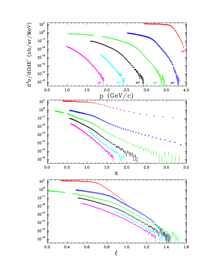
Figure 3.21: Cross section for all HMS angles as a function of $p$, $x$, and $\xi$.

The other improvement involved binning the data in different variables. Once we have applied the bin centering correction, we are looking at the cross section at a fixed valued of $p$ and $\theta$. At that point, we can freely translate to any other desired variables that specify the kinematics. This means that if we start with variables other than $p$ and $\theta$, bin the data and apply acceptance and bin centering corrections, we can convert back to the desired $p$ and $\theta$ values. Thus, if we can replace $p$ with some other variable, over which the $\theta$ variation of the cross section is smaller, we can bin the data over $\theta$ and have a significantly smaller bin centering correction than when we use $p$ and $\theta$. Figure 3.21 shows the cross section for all of the angles as a function of $p$, $x$, and $\xi$. For fixed p, the cross section varies by a factor between 5 and 200 over the theta acceptance of the HMS ($\sim 3^{\circ}$, or roughly 1/2 to 1/3 of the spacing for the angles shown). This is what causes the large correction using the method of equation (3.14). The correction is especially large at the higher values of $p$, corresponding to the large $Q^{2}$ values which are of the most interest, and where the model cross section is least well known. For fixed values of $x$, the cross section variation over the HMS $\theta$ acceptance is typically a factor of 1.5 to 3, and is always $\mathrel{\raise 1.29167pt\hbox{$<$}\mkern-14.0mu\lower 2.58334pt\hbox{$\sim$}}10$. The $\theta$ variation for fixed $\xi$ is even smaller, usually less than a factor of 2, and is smallest at the high $Q^{2}$ values (corresponding to large scattering angles). Therefore, by binning in $\xi$ and $\theta$, and including the acceptance in the correction, rather than directly to the binned counts, we have a significantly smaller bin centering correction of the form:

$$\mbox{($\xi,\theta$) Binning Correction}=\frac{\sigma^{*}(\xi_{0},\theta_{0})\cdot\Delta\xi\cdot\Delta\theta}{\int_{\theta_{0}-\Delta\theta/2}^{\theta_{0}+\Delta\theta/2}\int_{\xi_{0}-\Delta\xi/2}^{\xi_{0}+\Delta\xi/2}A(\xi,\theta)\cdot\sigma^{*}(\xi,\theta)d\xi d\theta},$$ (3.16)

where $\sigma^{*}$ is now the differential cross section $\frac{d\sigma}{d\xi d\Omega}$, rather than $\frac{d\sigma}{dpd\Omega}$.

Figure 3.22 shows the size of the bin centering correction for 30^∘, taking fixed $p,x,$ or $\xi$ and binning over a $\pm$1.4^∘ bin. For each variable, the correction was calculated using two models in order to estimate the model dependence. The top line is using our final model of the cross section (see section 3.4). The bottom line comes from adding an additional $Q^{2}$ dependence to the model. The standard model is typically within 10% of the data (and always within 30%), and has small ($<$10%) variations in the ratio of data to model when comparing different angles. The modified model ($\sigma^{*}=\sigma\cdot\frac{Q^{2}}{\langle Q^{2}\rangle}$) introduces large discrepancies between the model and data (up to a factor of 5), and introduces a large angular variation in the ratio of data to model. While this severely overestimates the uncertainty in the $\theta$ dependence of the model, it still leads to a small uncertainty in the correction when taking fixed $\xi$.

Figure 3.22: Bin centering corrections at 30^∘ for a $\pm$1.4^∘ bin. The dotted line is the correction at fixed $p$, dashed is for fixed $x$, and solid is for fixed $\xi$. The top line in each case represents the correction calculated using the standard cross section model. The bottom line is for the model with a large $Q^{2}$ dependence, used to estimate the uncertainty in the correction.

In the real data, the acceptance does not always include a symmetric region in $\theta$ about the central value in $\xi$. The acceptance of the spectrometer is a roughly rectangular region in $\delta$ and $\theta$. A fixed $\xi$ bin is a roughly straight line through the $\delta$,$\theta$ acceptance region, as shown in figure 3.23. For a value of $\xi$ corresponding to $\delta=0$, $\theta=\theta_{0}$, the entire $\theta$ range is included in the bin. For $\xi$ bins corresponding to high or low values of $\delta$ (at the central angle), only part of the $\theta$ acceptance lies within the spectrometer acceptance. Therefore, the bin centering corrections are largest at the edge of the momentum acceptance, where a bin of fixed $\xi$ only includes half of the $\theta$ acceptance. Instead of comparing the average cross section to the central value, we are comparing the average to the extreme value, and so the maximum bin centering corrections occur at the edge of the acceptance. Figure 3.24 shows the correction for a bin extending from 30^∘ to 31.4^∘, and represents the maximum possible correction (and maximum uncertainty) for the 30^∘ data.

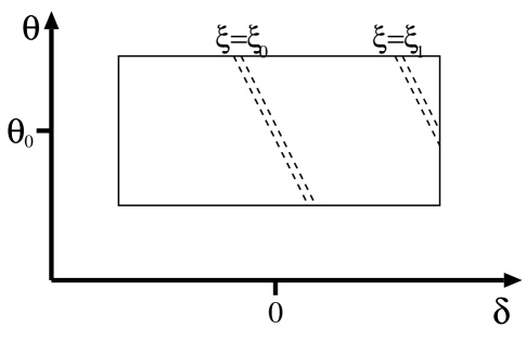
Figure 3.23: Fixed $\xi$ bins within the rectangular $\delta$-$\theta$ acceptance of the spectrometers. For central $\xi$ bins, the entire range of the $\theta$ acceptance is included in the bin. For the highest and lowest values of $\xi$, only half of the $\theta$ acceptance lies within the $\theta$ bin.

Figure 3.24: Bin centering corrections at 30^∘ for bin from 30^∘-31.4^∘. The dotted line is the correction at fixed $p$, dashed is for fixed $x$, and solid is for fixed $\xi$. The top line in each case represents the correction calculated using the standard cross section model. The bottom line is for the model with a large $Q^{2}$ dependence, used to estimate the uncertainty in the correction.

We apply an overall 1% systematic uncertainty in the cross section due to the bin centering correction. In addition, we apply an additional systematic uncertainty equal to 10% of the correction made. The maximum bin centering correction (for 15^∘, very low $\nu$) is 20%, leading to a 2% uncertainty in the correction (in addition to the 1% overall uncertainty).

Because the correction for the cross section variation over the $\xi$ bin is small, it is a good approximation to separate the binning centering correction into two pieces. By separating the $\xi$ and $\theta$ bin centering corrections, the corrections involve one dimensional integrals over the model cross section, rather than a two-dimensional integral. This significantly reduces the time required to calculate the correction.

In order to check the acceptance and bin centering correction, runs with significant overlap in momentum were taken. This allows us to have multiple measurements of the same cross section, taken in different regions of the spectrometer. Figure 3.25 shows the cross sections (in arbitrary units) from three runs with central momentum settings of 2.06, 2.20, and 2.36 GeV/c. It also shows the difference between the fit and the individual points as a function of $\delta$. The typical deviations from the fit are consistent with statistical uncertainties of the individual points ($\chi^{2}_{\nu}$ = 1.10 for 72 degrees of freedom), and a systematic uncertainty of 1% is applied to the acceptance at the peak value. Figure 3.26 shows overlapping runs for the SOS, at central momentum settings of 1.43, 1.56, and 1.70 GeV/c. For the SOS, the average residual is somewhat larger than expected from the statistics of the points ($\chi^{2}_{\nu}$=1.31 for 65 degrees of freedom), and the systematic uncertainty is somewhat larger (1.3% at the center of the acceptance)

Figure 3.25: Normalized yield and fractional deviations for overlapping HMS runs at 30^∘, p=2.06, 2.20, and 2.36 GeV/c.

Figure 3.26: Normalized yield and fractional deviations for overlapping SOS runs at 30^∘, p=1.43, 1.56, and 1.70 GeV/c.

The data is cut when the acceptance for a $\xi$ bin falls below 50% of the maximum acceptance. The uncertainty associated with the acceptance is 1% (1.3% in the SOS) combined in quadrature with 4% of the difference between the acceptance for the bin and the maximum acceptance. Therefore, for a bin with an acceptance of 0.5, the systematic uncertainty is $(.01^{2}+(.04*(1-0.5))^{2})=2.2$%. In $\delta$ and $\theta$, the acceptance is roughly rectangular, and falls from 1 to 0 very quickly. Where the acceptance drops very rapidly, the Monte Carlo is very sensitive to small offsets or differences in resolution. Therefore, the uncertainty is large for a $\delta$ bin at the edge of the acceptance. However, when the data is taken as a function of $\xi$, the decrease in the acceptance comes mainly from the fact that the kinematic transformation between $\xi$ and $\delta$ means that only a certain portion of the $\xi$ bin has acceptance. Because the fraction that is populated comes from the mapping between $\xi$ and $\delta$ rather than losses at the edges of the spectrometer, it is less sensitive to any small offsets or resolution differences. Therefore, the uncertainty in acceptance correction is relatively insensitive to the size of the correction, and even for an acceptance of 0.5 (which leads to a 100% correction in the cross section), the uncertainty is small.

3.3.10 Radiative Corrections

The measured cross sections are also corrected in order to remove the effects of internal and external bremsstrahlung and energy loss in the target. The radiative corrections were applied using the same procedure as was used in the NE3 experiment[34]. Radiative effects are applied to a model cross section, using the radiative correction calculations of Stein et al.[66], which are based on the work of Mo and Tsai [67] and Tsai[68]. In addition, energy loss of the electron in the target, and in the spectrometer entrance window are applied, in order to reproduce the cross section measured in the experiment. The corrected model is compared to the measured cross section, and the model cross section is modified to improve the agreement. This procedure is repeated until the radiative model is consistent with the data. The radiative correction for each point is determined by comparing the model before and after the radiative effects have been applied. The measured cross sections are then multiplied by the ratio of the radiative model to the non-radiative model in order to remove the effect of the radiative losses.

The model used was the sum of a modified $y$-scaling model of the quasielastic cross section and a convolution calculation for the deep inelastic cross section [69]. The model is described in detail in section 3.4. After each iteration, the model is multiplied by a smooth function of $W^{2}$, the missing mass, in order to improve agreement with the model. At each step of the corrections procedure the model non-radiative cross section is of the form:

$$\sigma_{nr}^{*}=f_{i}(W^{2})\cdot(\sigma_{qe}^{*}+\sigma_{dis}^{*})$$ (3.17)

Initially, we start with no correction to the model cross section, i.e. $f_{0}(W^{2})=1$. After applying the radiative effects to the model, the radiated model is compared to the measured cross section, and the model is adjusted by modifying the function $f$ at the points where we have data ($W_{n}^{2}$):

$$f_{i}^{*}(W_{n}^{2})=f_{i-1}(W_{n}^{2})*\frac{\sigma_{meas}(W_{n}^{2})}{\sigma_{r}^{*}(W_{n}^{2})}.$$ (3.18)

$f_{i}^{*}(W_{n}^{2})$ is then smoothed using a cubic smoothing spline calculated using CUBGCV[70]) in order to generate $f_{i}(W^{2})$ for the next iteration. This procedure is complete when the radiated model is consistent with the data, i.e. when $\chi^{2}_{\nu}\leq 1$, where:

$$\chi^{2}=\sum_{i=1}^{n}\frac{(\sigma_{meas}(W_{n}^{2})/\sigma_{r}^{*}(W_{n}^{2}))-1}{(\delta\sigma_{r}^{i}/\sigma_{r}^{i})^{2}}.$$ (3.19)

In order to examine the model dependence of the correction, the procedure was tested with three different models. Figure 3.27 shows the three models used. The solid line is the standard model, described in section 3.4. The dashed line is for a model with the ‘smearing’ of the nucleon structure functions removed ($F_{2}^{A}=ZF_{2}^{p}+NF_{2}^{n}$, no convolution with $f(z)$), and with the quasielastic ($y$-scaling) model calculated for an energy loss 20% farther from the quasielastic peak, and with a 20% increase in the normalization. This leads to a model where the quasielastic and resonance peaks are significantly narrower and higher, and the cross section is not as smooth as a function of $\nu$. The dashed line is for an initial model with a flat cross section (10 nb/Mev/sr). Figure 3.28 shows the radiative correction factor for the 15^∘ data using three different initial models. The top figure is the radiative correction factor ($\sigma_{nr}^{*}/\sigma_{r}^{*}$) for the standard model used to analyze the data. The bottom figure shows the correction for two different models, divided by the correction for the standard model. The dashed and dotted lines correspond to the modified models shown in figure 3.27. For both models, over a range of radiative correction factor from 1.2 to 1.5, the calculated radiative correction factors have only a small model dependence.

Figure 3.27: Three different cross section models used to test the radiative correction procedure. The solid line is the standard model (for Iron at 15^∘). The dashed line has the ‘smearing’ of the nucleon structure functions removed for the inelastic contributions, and decreases the width of the quasielastic peak by 20%, keeping the normalization fixed. The dashed line is a constant cross section of 10 nb/MeV/sr.

Figure 3.28: Radiative correction factor for three different input models. The top curve is the correction factor for the three model shown in figure 3.27. The bottom curve shows the correction factor divided by the value for the standard model used in the analysis.

In addition to checking the model dependence, we can test the external radiative correction procedure by examining data from targets of different thicknesses, and insuring that the corrected cross sections are identical. Figure 3.29 shows the cross section for data taken at identical kinematics with the thin and thick Iron targets. The thin target is 1.54% of a radiation length, and has a radiative correction of between 12% and 24%. The thick target (5.84% of a radiation length) has a correction that varies between 20% and 45%. Therefore, the measured cross sections differ by $\sim$10-20%. However, after applying the radiative corrections, the cross sections are in good agreement. The ratio of thick to thin is 1.0078$\pm$0.0052, which is smaller than the uncertainty in the ratio of the target thicknesses. Another run, taken at different kinematics and with significantly lower statistics, gives a ratio of 1.0326$\pm$0.014. From the model dependence, and tests with different target thicknesses, we assign a 2.5% systematic uncertainty to the radiative corrections.

Figure 3.29: Cross section before and after radiative corrections for two different Iron targets. The hollow points are the measured cross section, and the solid points are the cross section after the radiative corrections have been applied. The boxes are data taken on the thick iron target, and the diamonds are for the thin iron target. The right figure shows the ratio of cross sections, after radiative corrections have been applied.

Because the iterative procedure is applied to each kinematic setting for the experiment, it is somewhat sensitive to the fit to the cross section at the low-$\nu$ value of the data range. For values of $\nu$ below the range of the data, the correction to the model is kept constant at the value from the lowest $\nu$ point available. Therefore, fluctuations in the lowest $\nu$ points can have an effect on the model cross section over a large range of $\nu$ values. The only places where there are large corrections to the model are at low $\theta$ and low $\nu$. In this region, the cross section drops rapidly with decreasing $\nu$. Therefore, the strength coming from this region in the radiative correction is small, and the model dependence is not very large. However, while the effect is always relatively small (within the systematic uncertainties we have assigned), the fluctuations in the data for the low $\nu$ points can cause a systematic error for a large range of the data at that kinematic setting. In addition, correcting each kinematic setting independently means that the error made may be nearly constant for a single momentum and angle setting, but then jump at the few percent level between different kinematic settings. This becomes important when comparing the data taken on different targets. When comparing the structure function per nucleon for the different targets, the differences are typically small ($\mathrel{\raise 1.29167pt\hbox{$<$}\mkern-14.0mu\lower 2.58334pt\hbox{$\sim$}}$10%). If one takes the ratio of structure functions as a function of $x$, the systematic uncertainties can lead to a false $x$ dependence. While the errors made are within the systematic uncertainties assigned, it is important to remember that the systematic uncertainties are not uncorrelated between the different $\nu$ values, nor do they cause an overall offset or normalization to the data set. An overall systematic uncertainty (a normalization or efficiency problem) would cancel when taking the ratio of the target, and even if there was only a partial cancellation, it would not introduce any $x$ dependence to the ratios. A systematic uncertainty that is uncorrelated between different points would make it more difficult to determine the $x$ dependence, but would not tend to introduce systematic differences in the target comparison in different regions of $x$.

The radiative correction procedure will be modified when the deuterium data is analyzed in order to reduce this effect. The plan is to combine all data at a single spectrometer angle with the appropriate normalization and apply the radiative correction to all of the data at once. This means that the extrapolation beyond the range of the data will only be important at the lowest $\nu$ values, where the cross section falls rapidly, and there is very little strength gained from lower $\nu$ values. This will produce a smooth radiative correction over the entire momentum range and eliminate the ‘jumps’ in the extracted cross section coming from the variations in the radiative correction factor at different momentum settings.

3.3.11 Coulomb Corrections

After the incoming electron passes through the atomic electrons of the target atom, it sees a bare nucleus, and is accelerated by the electric field of the nucleus. This acceleration leads to an increase in the energy of the incoming electron, and a decrease in the energy of the scattered electron. This means that the energy of the initial and scattered electron at the scattering vertex is not the same as the energies determined by measurements of the beam energy and the scattered electron momentum. This change in kinematics can have a significant effect on the measured cross section. In addition, the electric field of the nucleus can lead to a deflection of the electron when the scattering occurs at the edge of the nucleus. This deflection of the electron means that at fixed spectrometer angle, we are measuring over a range of scattering angles.

We estimate the effect of the Coulomb energy correction by calculating the cross section from our model (section 3.4) with and without the energy shift due to the Coulomb acceleration. In order to estimate the energy shift, we treat the nucleus as a uniform sphere of radius $R_{0}$. Then, the electric potential for a point $r$ inside of the nucleus ($r<R_{0}$) is given by:

$$V(r)=-\frac{Ze}{8\pi\epsilon_{0}R_{0}}\left(3-\frac{r^{2}}{R_{0}^{2}}\right).$$ (3.20)

with $V(\infty)$ defined to be zero. Outside of the electron cloud, the potential from the nucleus is canceled by the potential from the electrons. However, at typical electron distances, the potential is $\sim$10^-4 of the potential at the surface of the nucleus. We thus neglect the shielding by the atomic electrons, and the energy change for the electron at the surface of the nucleus is:

$$\Delta E(R_{0})=eV(R_{0})=\frac{Ze^{2}}{4\pi\epsilon_{0}R_{0}}=1.44MeV\frac{Z}{R_{0}}.$$ (3.21)

Assuming that the scattering occurs uniformly throughout the nucleus, we calculate the average energy shift for the scattering:

$$\langle\Delta E\rangle=\frac{\int_{0}^{R_{0}}V(r)r^{2}dr}{\int_{0}^{R_{0}}r^{2}dr}=\frac{6}{5}\Delta E(R_{0}).$$ (3.22)

Table 3.5 gives the values for $R_{0}$, $\Delta E(R_{0})$, and $\langle\Delta E\rangle$ used in the correction. Using this average energy correction, we estimate the correction to the cross section by calculating the cross section for our model (section 3.4) at the nominal kinematics, and with the Coulomb energy correction applied ($E\rightarrow E+\langle\Delta E\rangle,E^{\prime}\rightarrow E^{\prime}+\langle\Delta E\rangle$, and $\nu$ remains constant at the point of interaction). We take the modification of the cross section model as our correction to the data for the Coulomb energy correction. The correction is roughly proportional to $\langle\Delta E\rangle$, and averages 2% for Carbon, 5.5% for Iron, and 9.8% for Gold. The largest corrections to the data occur at 74^∘, and are at most 6% for Carbon, 15% for Iron, and 24% for Gold.

Nucleus	$R_{0}$ [fm]	$\Delta E(R_{0})$ [MeV]	$\langle\Delta E\rangle$ [MeV]	RMS $p_{\perp}$ [MeV/c]
12C	3.23	2.67	3.2	1.5
56Fe	4.85	7.72	9.3	4.4
197Au	6.88	16.53	19.8	9.8

Table 3.5: Effective radius, Coulomb energy correction (at surface and averaged over the nucleus), and RMS transverse momentum kick for the target nuclei. The radius is taken from [71], and is the effective radius for the nucleus, assuming a spherical nucleus with uniform charge density.

In addition to the energy change for the initial and scattered electron, the Coulomb field of the nucleus will lead to a deflection of the electron. The maximum deflection occurs when the electron grazes the nucleus. In this case, the incoming electron can be approximated by integrating the component of the force transverse to the electron direction, neglecting the change in the trajectory. In this case, the transverse ‘kick’ received by the electron is:

$$\Delta p_{\perp}=\int_{-\infty}^{0}F_{\perp}dt=\frac{1}{c}\int_{-\infty}^{0}F_{\perp}dr_{\parallel}=\Delta E(R_{0})/c$$ (3.23)

The worst case is for gold, where $\Delta p_{\perp}$=16.5 MeV/c for an electron at $r_{\perp}=R_{0}$. This leads to an angular deflection of $\Delta\theta=\Delta p_{\perp}/p_{beam}=4.1$ mr, which is much larger than the uncertainty in the $\theta$ reconstruction. In addition, there will be a transverse kick of similar magnitude to the scattered electron. Because the scattered electron energy can be much lower than the beam energy (as low as $\sim$600 MeV), the deflection can be much larger. A Monte Carlo calculation was used to determine the distribution of $\Delta p_{\perp}$ for events generated uniformly within the nucleus. Figure 3.30 shows the distribution of $\Delta p_{\perp}$ for Carbon, Iron, and Gold. The distribution is relatively flat, and was approximated by a flat distribution with a width chosen to match the RMS value of the calculated distribution. The correction to the cross section was determined by comparing the model cross section at the measured angle to the average value over the $\theta$ range determined by combining the angular range of the incoming electron ($\Delta\theta=\Delta p_{\perp}/p_{beam}$) with the angular range of the scattered electron ($\Delta\theta^{\prime}=\Delta p_{\perp}/p^{\prime}$). The angular range can be large for high $\nu$ (low $E^{\prime}$), but the cross section has the greatest $\theta$ variation at low $\nu$, and the correction is never very large. While the angular deflection range is proportional to the $\Delta p_{\perp}$ kick, the correction grows at least as fast as the square of the angular range. The correction is $\mathrel{\raise 1.29167pt\hbox{$<$}\mkern-14.0mu\lower 2.58334pt\hbox{$\sim$}}$5% for Gold, $\mathrel{\raise 1.29167pt\hbox{$<$}\mkern-14.0mu\lower 2.58334pt\hbox{$\sim$}}$2% for Iron, and $\mathrel{\raise 1.29167pt\hbox{$<$}\mkern-14.0mu\lower 2.58334pt\hbox{$\sim$}}$0.5% for Carbon, and has the opposite sign as the correction for the energy change of the electrons (except when the correction is very small).

Figure 3.30: $\Delta p_{\perp}$ distribution for electrons due to the Coulomb field of the nucleus. The distributions are approximated as uniform distributions with $\Delta p_{\perp}^{max}$ of 2.7 MeV/c for Carbon, 8.0 MeV/c for Iron, and 17.2 MeV/c for Gold.

Figure 3.31 shows the correction for Iron, as a function of angle. The crosses show the correction to the model when the coulomb energy correction is applied, the diamonds show the correction to the model coming from the deflection of the electrons, and the circles show the combined effect. For Gold the correction is roughly twice as large, and for Carbon, the total correction is roughly one third of the correction for Iron. The Coulomb correction for the Hydrogen elastic scattering data has a negligible effect on the cross section, and a small effect effect on the measured position of the $W^{2}$ peak. However, the effect was small enough that it does not significantly affect the conclusions of the spectrometer momentum and beam energy calibration.

Figure 3.31: Coulomb corrections for the Iron data. The crosses represent the change in the model cross section when $\Delta E$ is applied. the diamonds are the correction when the angular deflection is applied, and the circles are the combined effect. The correction is roughly twice as large for Gold, and one third of the size for Carbon. The multiple points at each angle represent different values of $\nu$. The corrections are largest for the lowest $\nu$ values.

The main source of uncertainty in the correction comes from the assumption that the nucleus can be modeled as a sphere with uniform charge distribution, and the uncertainty in the radius chosen for the sphere. In addition, it is assumed that the electron scattering occurs uniformly throughout the volume of the nucleus. However, the boost in electron energy will modify the cross section as a function of position from the center of the nucleus, leading to a slightly non-uniform distribution of events. We estimate that the uncertainty associated with modeling the nuclei as uniform spheres, and the choice of radius (given in table 3.5) is less than 8% of the correction. The model dependence in calculating the correction is less than 5% of the correction. Finally, the maximum difference in cross section between the center of the nucleus and the edge of the nucleus is $\sim$10% in Gold, $\sim$7% in Iron, and $\sim$2-3% in Carbon. We assume that the average effect of including the cross section weighting is always less than half of the maximum cross section variation, and use half of this value as the overall uncertainty. In the current analysis, we use the maximum correction to determine the overall systematic uncertainty for each target, giving an upper limit for the uncertainty in the extracted cross section of 0.6% for Carbon, 1.7% for Iron, and 2.8% for Gold. This uncertainty is fairly small relative to the other systematic uncertainties (typically 3.5-4.0%). With a more careful comparison of different models for the charge distribution and the effects of neglecting the cross section weighting, these uncertainties should be significantly reduced from their present values, and should have a negligible effect on the total systematic uncertainties for Carbon and Iron, and a small effect for Gold.

As part of the radiative correction procedure, the model cross section is corrected for radiative effects, and the scattering kinematics are corrected for energy loss in the target and in the spectrometer vacuum window. However, while the coulomb correction could also be applied as part of the radiative correction procedures, there are two advantages to making a separate correction. First, we need to apply the same correction to the data from previous measurements [34, 35, 25] in order to compare results (the analysis of the NE3 data and the inclusive analysis of the NE18 data did not include coulomb corrections except for the extrapolation to nuclear matter [72]). Only the Iron data is compared to the SLAC results, and the average coulomb correction is $\sim$4%, and the maximum correction is 10%. In addition, while the energy change due to the coulomb correction is applied as a shift in energy, the deflection of the electron due to the coulomb field leads to an averaging of the cross section over a range in $\theta$. Including this in the radiative correction procedure would significantly increase the CPU time required to determine the radiative corrections.

3.4 Cross Section Model

For the bin centering corrections and the radiative correction, we need a model of the cross section. Because the calculation of these corrections is CPU intensive, we need a model that can be calculated quickly. The radiative corrections are calculated using an iterative procedure, which corrects the model at each iteration, and is relatively insensitive to errors in the model. However, the bin centering correction is not done iteratively, and the model must be in good agreement with the data in order for the correction to be made with a small uncertainty. We break up the model into two pieces, one to model the inelastic cross section, and one to measure the quasielastic cross section. For both pieces, we start with a theoretical model of the cross section, and make adjustments to improve the agreement with our data.

3.4.1 Model of the Inelastic Contributions.

The model used for the inelastic cross section is based on the convolution procedure of Benhar et al. [69], using the fits to the proton and neutron structure function. The procedure is a convolution of the nucleon distribution function and the nucleon structure function. The nucleon distribution function is $f_{A}(z,\beta)$, where $z$ is the momentum of the nucleon in the nucleus (0$<z<$A), and $\beta=|q|/\nu$. The nucleon distribution function is the probability that the nucleon will have a fraction $z$ of the momentum of the nucleus, and is defined as:

$$f_{A}(z,Q^{2})=z\int dEd^{3}kS(k)\delta\left(z-\frac{E\nu-\vec{k}\vec{q}}{m\nu}\right)$$ (3.24)

where $S(k)$ is the relativistic vertex function (which can be approximated by the non-relativistic structure function, ($S(E,\vec{k})\approx\frac{m}{k_{0}}S(E_{s},p_{0})$). This is convoluted with the nucleon structure function, $F_{2}^{N}(x,Q^{2})$, evaluated at $x$ corresponding to the fraction of the nucleon’s momentum carried by the struck quark. The nuclear structure function is then :

$$F_{2}^{A}(x,Q^{2})=\int_{x}^{A}f_{A}(z,\beta)F_{2}^{N}(x/z,Q^{2})dz$$ (3.25)

where $\beta=|q|/\nu$. Values of $f_{A}(z,\beta)$ were provided by Benhar, calculated for nuclear matter. The proton and neutron structure functions were taken from Bodek et al. [73] and corrected for the EMC effect using a parameterization from SLAC experiment E139 [74, 75]. The values of $f_{A}(z,\beta)$ were calculated for nuclear matter. The model was modified by lowering $\beta$ in order to better match the data in the DIS region and a calculation by Simula [76, 77] for the inelastic contributions in Iron for $0.5<x<2.2$ (see section 5.1 for details on the calculation) . Part of the improvement may come from the fact that lowering the value of $\beta$ reduces the width of $f_{A}(z)$, and may take into account some of the difference between the convolution function calculated for nuclear matter and the convolution function for finite nuclei. The cross section model was more sensitive to a modification in $\beta$ in the high-$x$ region, where $\nu$ is low. Taking $\beta=|q|/(\nu+0.5GeV)$ gave significant improvement in the agreement with the calculation by Simula, and also improved the agreement with the data in the DIS region. A further $Q^{2}$ dependent correction was applied in order to improve the agreement between the model and data in the DIS region, where the cross section was approximately correct at low $Q^{2}$, and too low at higher $Q^{2}$. Thus, the cross section calculated from the convolution model (with modified $\beta$) was multiplied by $[0.8+0.42*exp(-Q^{2}/2.0)]$ in order to match the data.

3.4.2 Model of the Quasielastic Contributions.

For the quasielastic contribution, we use a $y$-scaling model, with modifications at lower values of $Q^{2}$ designed to reproduce the cross section in the region where the final-state interactions are large. We use the parameterization from ref. [78] for $F(y)$:

$$F(y)=\frac{Ae^{-a^{2}y^{2}}}{\alpha^{2}+y^{2}}+Be^{-b|y|}.$$ (3.26)

The cross section is then just:

$$\frac{d^{3}\sigma}{dE^{\prime}d\Omega}=F(y)\cdot\bar{\sigma}$$ (3.27)

where $\bar{\sigma}$ comes from Eq. (4.3). The parameters $a,b,\alpha,A,$ and $B$ were chosen to reproduce the data, and were not required to satisfy any normalization condition. The values of the parameters used are given in Table 3.6, with $F_{0}=A+B$ replacing $A$ as one of the parameters.

Target	$F_{0}$	$B$	$a$	$b$	$\alpha$
	GeV-1	GeV-1	(GeV/c)-1	(GeV/c)-1	GeV/c
Carbon	3.3	0.40	3.88	10.0	0.140
Iron	2.8	0.40	3.88	10.0	0.140
Gold	2.5	0.40	3.88	10.0	0.140

Table 3.6: Parameters Used in the $y$-scaling Model of the Quasielastic Cross Section. $\alpha,a,b,B,$ and $F_{0}=A+B$ are fitted to the data, and used in equation 3.26. $a,b,\alpha,$ and $B$ were nearly independent of the target, and were fixed using the Iron data. $F_{0}$ was then fit for all nuclei.

Comparing the data to the model of the inelastic cross section plus the quasielastic cross section revealed some discrepancies in the model. At low angles, the $F(y)$ distribution was wider in the data than in the model. The normalization between the data and model also varied as a function of $\theta$. The parameters $a$ and $F_{0}$ were made functions of $\theta$ in order to improve the agreement:

$$a(\theta) = \frac{a}{1+(\frac{\theta-48^{\circ}}{50.81})^{4}}\;\;\;\;\;\;\;\mbox{for}\;\theta<48^{\circ}$$ (3.28)

$$F_{0}(\theta) = F_{0}\cdot(1.15-0.0068(\theta-15^{\circ})).$$ (3.29)

This gave good agreement between the data and model except for an underestimate of $F(y)$ near $y$=-0.6. A small correction was made by multiplying $F(y)$ by the following correction factor:

$$1+Ae^{-\frac{(y-y_{0})^{2}}{2\sigma^{2}}},$$ (3.30)

where $y_{0}$=-0.6 GeV/c, $\sigma$=0.12 GeV/c, and

$$A=\mbox{max}\;\left(0,40\cdot\left(\frac{1}{\theta}-\frac{1}{53^{\circ}}\right)\right).$$ (3.31)

Finally, by comparing the model to the full calculations from Simula, and by comparing the total model cross section (DIS + QE) to the data, it was clear that the $y$-scaling model was underestimating the cross section at $|y|\mathrel{\raise 1.29167pt\hbox{$<$}\mkern-14.0mu\lower 2.58334pt\hbox{$\sim$}}0.2$ GeV/c. The model was modified by rescaling $y$ near $y=0$, and restoring it for values of $y$ approaching 0.2 GeV/c. The final model used $F(y^{\prime})$, where:

$$y^{\prime}= 0.65y \mbox{for}\;0<|y|<0.05$$ (3.32)

$$y^{\prime}= 0.65y\left[1+\frac{0.35}{0.15(|y|-.05)}\right] \mbox{for}\;0.05<|y|<0.2$$ (3.33)

$$y^{\prime}= y \mbox{for}\;|y|>0.2.$$ (3.34)

While there is no theoretical justification for the exact forms of any of these corrections, they significantly improve the agreement between the model and the data. As long as they are smooth corrections in $\theta$, and reproduce the $\theta$ dependence of the cross section at each spectrometer angle, they should do a sufficient job of determining the $\theta$ bin centering correction. For the radiative correction, radiative effects are applied to the model, and the result is compared to the measured data. The model is then corrected to take this difference into account, and the procedure is repeated. Therefore, the radiative corrections are insensitive to small changes in the model. Figure 3.32 shows the measured Iron cross section versus the model cross section ($y$-scaling for the quasielastic plus the inelastic convolution model).

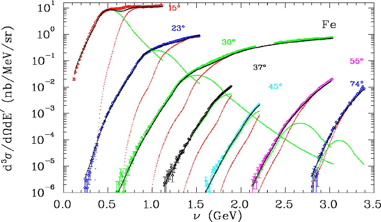
Figure 3.32: Measured cross section versus model values for Iron. The dotted line is the inelastic contribution from the convolution model, the dashed line is the quasielastic (modified $y$-scaling) model, and the solid line is the sum.

3.5 Calibration Data From Elastic Electron-Proton Scattering

H(e,e’) elastic scattering data was taken at each angle in order to check the beam energy and spectrometer momentum calibration, and to check the absolute cross section normalization of the spectrometers. From the High Momentum Spectrometer (HMS) elastic results, the beam energy was found to be consistent with the value measured in the Hall C Arc and the known beam energy drift during the run. (see section 2.3.3).

The elastic scattering data cross section was measured at each angle in order to check the absolute normalization of the measured cross sections. These runs were analyzed, with the standard tracking and particle identification cuts applied. A cut was placed around the elastic peak, and the number of counts was corrected for deadtime, tracking and trigger efficiencies. In order to remove counts coming from the aluminum endcaps of the hydrogen target, data was taken from a dummy target of identical length. The dummy target has aluminum entrance and exit windows at the same position as the hydrogen target, but the dummy windows are 9.23 times thicker. The counts measured from the dummy target were corrected for the difference in aluminum thickness and for the difference in total charge measured. These counts were subtracted from the measured counts in the elastic peak. The aluminum background varied between 2% and 7% of the total number of counts in elastic peak.

The expected number of counts was determined by running the Hall C Monte Carlo program SimC. This code was modified from the Monte Carlo used for analysis of the SLAC experiment NE18 [79, 80]. The models of the SLAC spectrometers were replaced with the HMS and SOS Monte Carlo models used to determine the spectrometer acceptances (see section 3.3.8), and the target and scattering chamber geometry were modified to reflect the CEBAF setup. Electrons are generated randomly within the acceptance of the HMS, and the kinematics for the corresponding proton are determined. The events are weighted by the cross section for the generated kinematics, and multiple scattering and radiative effects are applied to the events. After adequate statistics are generated (300k detected events), the Monte Carlo counts in the desired $W^{2}$ window are normalized to the total charge for the data. The Monte Carlo uses a dipole fit for the electric form factor, and the fit of Gari and Krümpelmann [81] for the magnetic form factor. For the HMS, the ratio of measured counts to Monte Carlo counts is shown in figure 3.33. There is a 1.05% systematic uncertainty that is uncorrelated between the different measurement (primarily from the charge normalization variation over time, cut dependence for the $W^{2}$ cut on the elastic peak, and possible localized boiling which is current and beam tune dependent). In addition, there is a 1.4% overall normalization uncertainty. A better calculation of the elastic cross section, using form factors fit to elastic data measured by Walker [82], was also compared to the data. In the figure, the crosses represent the ratio of the cross section based on the fit to Walker’s data to the cross section model used in the Monte Carlo. The elastic data is consistent with both model cross sections within the systematic uncertainties in the measurement and the uncertainty in the knowledge of the elastic cross section. Therefore, we do not assign any additional uncertainty on the overall normalization of the measured cross sections.

Figure 3.33: Ratio of measured elastic counts to expected counts. The solid circles are the HMS data. The statistical error bars and total uncorrelated errors are shown. The uncorrelated systematic uncertainty is 1.05%. There is an additional overall normalization uncertainty of 1.4%. The hollow circle is the SOS data at 55^∘. Only statistical errors are shown (the systematic uncertainty is $\sim$5%). The crosses represent the ratio of a fit to the Walker data [82] to the Monte Carlo value. The measured cross section is consistent with both the Monte Carlo cross section and the Walker data.

For the SOS, elastic data was taken at 48, 55, and 74 degrees. However, at 48 degrees, the elastic run was taken at a central momentum of 1.53 GeV/c. This means that the elastic peak (p=1.667 GeV/c at 48 degrees) occurs at the large $\delta$ side of the spectrometer. At the central angle, the elastic peak appears at $\delta$=+9.0%, and goes as far as $\delta$=16% within the angular acceptance of the SOS. Since we only use data with $|\delta|\leq 12\%$, and the reconstruction is unreliable outside of this region, we do not use this data for our normalization. In addition, at 1.53 GeV/c, there is an additional uncertainty in the SOS momentum value, due to a non-linearity in the momentum versus current relations for the magnets. This would lead to an additional uncertainty in the measured cross section. At 74 degrees, there is a non-negligible background from secondary electrons, which cannot be subtracted out because we did not take positive polarity data from hydrogen. While we can estimate the background by looking at the counts above the elastic peak, the uncertainty in the knowledge of the shape of the background underneath the elastic peak leads to an additional systematic uncertainty in the cross section ($\sim$3%). In addition, the total statistics at 74 degrees give only a 3-4% measurement of the cross section. Therefore, the 74 degree data is not very useful for normalizing the SOS cross section. At 55 degrees, the ratio of data to Monte Carlo was 0.984$\pm$0.011. While the result is slightly below the expected value, the discrepancy is within the statistical and systematic uncertainties of the measured cross section and the model cross section. However, comparisons of the HMS and SOS cross sections at 30^∘ and 55^∘ indicated that the SOS normalization was incorrect (see section 3.6). As a result, the SOS cross section was increased by 3%, with a 4% systematic uncertainty applied.

Figure 3.34 compares the data and the Monte Carlo distributions in $\delta$, $x^{\prime}_{tar}$, $y^{\prime}_{tar}$, and corsi$\equiv p-p(\theta)$ (the difference between the measured momentum and the momentum expected for elastic scattering at the measured angle) for the elastic run at 15^∘. The dummy target data has been subtracted in order to account for the background from the aluminum endcaps of the cryotarget. Figure 3.35 shows the same for the SOS at 55^∘. For both spectrometers, there is a small offset in $corsi$, but the offset is within the uncertainty caused by the uncertainties in beam energy, spectrometer momentum, and spectrometer angle. Because the small energy and angle offsets may be time or angle dependent, we cannot use the offset in $corsi$ to determine offsets for the energy or angle.

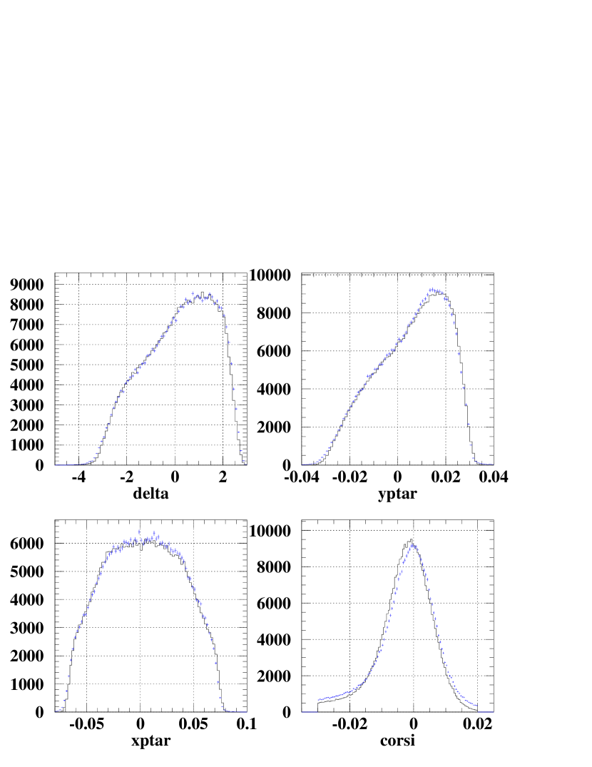
Figure 3.34: HMS 15^∘ elastic data versus Monte Carlo. ‘yptar’ and ‘xptar’ are the tangents of the in-plane and out-of-plane scattering angles at the target (‘yptar’=$y^{\prime}_{tar}$ and ‘xptar’=$x^{\prime}_{tar}$).

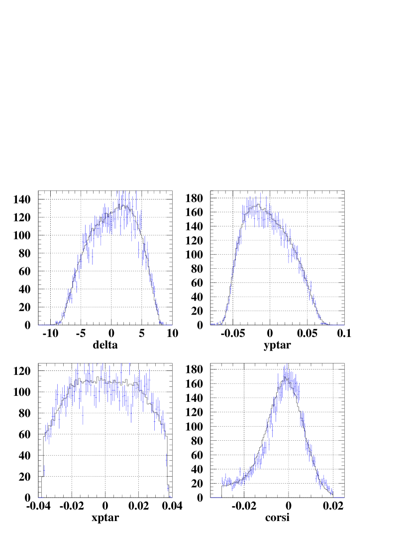
Figure 3.35: SOS 55^∘ elastic data versus Monte Carlo. ‘yptar’ and ‘xptar’ are the tangents of the in-plane and out-of-plane scattering angles at the target (‘yptar’=$y^{\prime}_{tar}$ and ‘xptar’=$x^{\prime}_{tar}$).

3.6 SOS Normalization

For the HMS, we have a good knowledge of the angle and momentum uncertainties from previous measurements, and from the elastic kinematics as a function of scattering angle. In addition, we can compare the elastic cross section to previous measurements at several angles, and the inclusive cross section to the NE3 measurement at kinematic nearly identical to the e89-008 30^∘ data. This gives us good checks of the normalization of the cross section for the HMS. Figure 3.36 shows the e89-008 HMS data at 30^∘, compared to the NE3 data. The NE3 data is corrected for the 50 MeV difference in beam energy between the two experiments, and divided by the e89-008 cross section. The e89-008 results are shown in order to indicate the size of the statistical uncertainty.

Figure 3.36: Comparison of NE3 and e89-008 cross sections at 30^∘. The curves are the NE3 and e89-008 data at 30^∘, divided by the e89-008 result. The errors shown are statistical only. The dashed line indicates the systematic uncertainty ($\sim$3.5% for both experiments). The ratio of cross sections (e89-008/NE3) is 1.014$\pm$.005%, which is well within the systematic uncertainty in the ratio ($\sim$5%).

For the SOS, the momentum and angle are not as well known, and we can only check the elastic normalization at 55^∘. Because the SOS has a lower maximum momentum ($p_{cent}<1.74$ GeV/c), we have data for $x>1$ only at 55^∘ and 74^∘, along with some low-$x$ data at 30^∘ which was used primarily for acceptance studies and detector calibration. In addition, because of the non-linearity in the SOS at higher momentum settings (see section 2.5.3), the high-$x$ data at 55^∘ has a large uncertainty in the scattering kinematics, in the region where the cross section varies most rapidly. Therefore, the data at 55^∘ adds very little to the HMS 55^∘ measurements. Therefore, we used the SOS data at 30^∘ and 55^∘ to determine the absolute normalization of the SOS cross section, and apply this normalization to the 74^∘ data.

Figures 3.37 and 3.38 compare the HMS and SOS cross sections at 30^∘ and 55^∘. For 30^∘, the SOS cross section is $\sim$0-3% lower than the HMS (depending on the value of $\xi$). For 55^∘, the SOS is $\sim$4-6% low compared to the HMS. The SOS elastic is 1.2% below the expected cross section at 55^∘. Averaging these offsets, we apply a 3% correction to the SOS cross section. This is a little high for the 30^∘ data, and a little low for the 55^∘ data, but is within the systematic uncertainties.

Because we have elastic calibration data only at 55^∘, and inclusive data only at 30^∘ (low $x$) and 55^∘, it is difficult to determine if the cross section normalization comes from errors in the efficiencies or errors in the kinematics (SOS momentum, angle, or beam energy). Therefore, we apply a cross section normalization to make the SOS agree with the HMS, and apply a systematic uncertainty based on the possible kinematic dependence of the normalization factor.

Figure 3.37: Comparison of HMS and SOS cross sections at 30^∘. The circles are the HMS cross section, divided by a fit to the HMS. The squares are the SOS data points, divided by the same fit. The SOS is in good agreement with the HMS at low values of $\xi$, and $\approx$3% low at larger $\xi$ values.

Figure 3.38: Comparison of HMS and SOS cross sections at 55^∘. The circles are the HMS cross section, divided by a fit to the HMS. The squares are the SOS data points, divided by the same fit. The SOS points are roughly 4% low at lower $\xi$ values, and $\approx$6% low at larger $\xi$ values.

The angle (and $\xi$) dependence of the observed HMS/SOS ratio indicates that the correction might be different at 74^∘. If the effect comes from an error in the tracking/PID/cut inefficiency, then it might be a function of momentum. If the difference comes from an offset in the spectrometer momentum or angle, then it will have an angle and momentum dependence. However, a shift in the kinematics large enough to modify the cross sections would also be large enough to shift the $W^{2}$ peak for the elastic measurement so that it would not be consistent with the elastic scattering. Therefore, the cross section difference must involve a combination of angle, momentum, and beam energy shifts, along with a possible normalization problem, in order to reproduce the cross sections and the elastic scattering kinematics. Because we cannot determine the cause of the discrepancy, we will determine the offset at 74^∘ assuming a fixed angle change, fixed momentum change, and fixed normalization, and assign an uncertainty to the 3% correction large enough to make the result consistent with any of these possibilities. A fixed momentum offset of 0.4% would correct the 30^∘ and 55^∘ data, and would lead to an offset in the 74^∘ measurement between 2% and 8% (at low and high values of $\xi$). A fixed angle offset of 2.0 mr leads to a correction at 74^∘ between 1% and 4%, and a fixed cross section normalization of 3% is the best value for the 30 and 55 degree data. Therefore, the correction to the 74^∘ data may vary between 1.5% and 8% over the $\xi$ range of the data, depending on the source of the normalization error. Therefore, we apply a 3% normalization correction to the SOS cross sections, and assign a systematic uncertainty of 4% to this correction.

3.7 Systematic Uncertainties

Table 3.7 summarizes the systematic uncertainties for the HMS and SOS. The uncertainties are discussed in the sections given in the table. The positron subtraction, kinematic uncertainties, and Coulomb corrections are discussed below. For the HMS, the systematic uncertainty is typically $\sim 3.5-4.0\%$, though it is somewhat larger at low $x$ and $Q^{2}$ values, where the bin centering correction has the largest uncertainties, at 55 degrees, where there is a significant uncertainty for the thick targets (up to 5%) due to positron subtraction, and at low energy loss (mostly at 15^∘ and 23^∘) where the uncertainty in beam energy and spectrometer momentum has the greatest effect on the cross section. The SOS has data only at 74 degrees, and the uncertainty comes primarily from the 4% uncertainty in the SOS normalization (see section 3.6), the uncertainty in the spectrometer momentum and angle, and the positron subtraction (which dominates the uncertainties for the thick targets).

	HMS	SOS	Section
Acceptance Correction	1.0-2.2%*	1.3-2.4%*	3.3.9
Radiative Correction	2.5%*	2.5%*	3.3.10
Target Track Cuts	0.5%	0.5%	3.3.2
Bin Centering Correction	1.0-2.2%*	1.0-1.6%*	3.3.9
PID Efficiency/Contamination	0.5%*	1.0-3.0%*	3.3.3
Charge Measurement	1.0%	1.0%	2.3.4
Target Thickness	0.5-2.0%	0.5-2.0%	2.4
Target/Beam position offsets	0.25%	0.25%	2.4.2
Tracking Efficiency	0.5%*	0.5%*	3.3.7
Hodoscope Trigger Efficiency	0.05%*	0.05%*	3.3.6
Normalization Uncertainty	0.0%	4.0%*	3.5,3.6
Combined Uncertainty	3.2-4.7%	5.3-6.7%
e+ Subtraction(55∘,74∘)	0-5%*	3-10%*	3.3.4
Kinematic Uncertainties	0.4-8.3%	1.2-4.5%	2.5.3,2.3.3
Coulomb Corrections	0.6-2.8%	0.6-2.8%	3.3.11

Table 3.7: Systematic Uncertainties in the extraction of $d\sigma/d\Omega/dE^{\prime}$. The positron subtraction and kinematic uncertainties are described in the text. Entries marked with a ‘*’ are items where a correction is made to the cross section, with the uncertainty as shown in the table. Unmarked entries are not used to correct the measured cross section. They only contribute the uncertainty.

The uncertainties given for the positron subtraction represent the uncertainty in the measurement of the positron background at 55^∘ (HMS) and 74^∘ (SOS). However, because the charge-symmetric background is nearly equal to the electron signal for the thick targets at 74^∘, the cross section from the negative polarity runs is reduced by a factor of two when the charge-symmetric background is subtracted. Therefore, any systematic uncertainties which are uncorrelated between the negative and positive polarity runs will increase (relative to the measured cross section) after the positron contribution has been subtracted. Because we measure the charge-symmetric background on just one or two targets for each kinematic setting, we make a fit to the $e^{+}$ cross section and use this for the subtraction. Therefore, most of the errors are uncorrelated between the measured electron data and the fit to the positron data, leading to an increase in the fractional uncertainty due to the systematic errors.

The kinematic uncertainties come from taking the uncertainties in the beam energy, spectrometer momentum, and spectrometer angle, and determining the error in the cross section due to these possible offsets. The error is determined by applying the offsets to the model cross section. For the HMS, the beam energy and spectrometer momentum offsets are the main source of uncertainty at low angles and low $\nu$, where a small energy or momentum shift can give a large (fractional) shift in the energy transfer, and where the cross section falls most rapidly as a function of $\nu$. At angles above 23^∘, the scattering angle offset is the main source of error, and the cross section uncertainty is typically $\mathrel{\raise 1.29167pt\hbox{$<$}\mkern-14.0mu\lower 2.58334pt\hbox{$\sim$}}$1% for low $\xi$ values, and 2-3% at high $\xi$ values, where the cross section is dropping rapidly. For the SOS, the spectrometer momentum and angle are not as well known as in the HMS, and the uncertainty is 1-2% at low $\xi$, and 3-4% at high $\xi$, coming mostly from the momentum and angle uncertainties.

The effect of the Coulomb field of the nucleus is corrected for in the analysis (section 3.3.11). 0.6

Figure 3.39 shows the statistical, systematic, and total uncertainties for the HMS data at 15^∘, 30^∘, and 55^∘ and the SOS data at 74^∘ for the Iron cross section. In general, the errors are dominated by the systematic uncertainties except for the lowest $\nu$ points at each angle. The additional uncertainty in the structure function arising from the uncertainty in $R=\sigma_{L}/\sigma_{T}$ is shown (see section 5.6).

Figure 3.39: The dashed lines show the statistical (long dash) and systematic (short dash) uncertainties in the measured cross section for Iron. The solid line is the total uncertainty (statistical and systematic added in quadrature). The dotted line shows the additional uncertainty in the extraction of the structure function due to the uncertainty in $R=\sigma_{L}/\sigma_{T}$ (see section 5.6). The systematic uncertainties coming from the Coulomb corrections (section 3.3.11) are not included. The error in the corrections is estimated to be less than 2.8% for Gold, less than 1.7% for Iron, and less than 1% for Carbon. The systematic error (3.5-4.5% for the HMS, 10-12% for the SOS) dominates the cross section for all but the lowest values of $\nu$ at each angle. The SOS has $\sim$5-6% systematic uncertainties in the measured counts, but because roughly half of the counts are subtracted as part of the charge-symmetric background, the systematic uncertainty is 10-12% of the post-subtraction electron cross section. Because the positron data is only taken on some targets and a fit to the $e^{+}$ cross section is made and subtracted from the negative polarity data, the systematic uncertainties are largely uncorrelated between the negative polarity data and the positron cross section that is subtracted.

All of the uncertainties shown in table 3.7 are included in the quoted systematic uncertainties for the data. However, there is some additional uncertainty for data at the lowest angles (15^∘ and 23^∘) in the region of the quasielastic peak. The cross section model, choice of binning variables, and radiative corrections have been optimized to have a small model dependence and systematic uncertainty in the regions where the cross section is relatively smooth and on the low energy-loss side of the quasielastic peak. At low $Q^{2}$, where the quasielastic peak is clearly distinguishable, there is a greater model dependence to the binning corrections. For the bin centering correction, the problem arises because we bin in $\xi$. At higher values of $Q^{2}$ or $\xi$, the cross section is very smooth as a function of $\theta$ at fixed $\xi$. However, in the region of the resonances and at the center of the quasielastic peak, the data has a smoother $\theta$ dependence for fixed $W^{2}$ than for fixed $\xi$. Because the focus of this experiment was higher $Q^{2}$ and higher $\xi$, it was decided to analyze all of the data in the same fashion, even though it introduces additional uncertainties in the region. For runs taken on either side of the quasielastic peak at 15^∘ and 23^∘, the overlapping data on top of the quasielastic peak do not agree perfectly. However, the error made by binning in $\xi$ rather than $W^{2}$ is only large at the edge of the acceptance, and the error made should be roughly opposite for data at the high-$\delta$ region of the acceptance and low-$\delta$ region. Therefore, while the overlapping data do not agree, the errors made should at least partially cancel when the runs are combined. Because it is difficult to determine the exact size of the model dependence, and because the errors made should at least partially cancel when the runs are combined, we do not assign an additional uncertainty to this regions, but note that the model dependence for our analysis procedure could lead to a somewhat larger error in this region. Figure 3.40 shows the cross section near the quasielastic peak at 15^∘, for measurement with central momentum settings of 3.21 GeV/c and 3.76 GeV/c. In the region of overlap, the two curves differ by $\sim$5%, which is within the assigned systematic uncertainty in the difference. Because the averaging the two sets of data will reduce the error made, any additional systematic uncertainty arising from the additional model dependence in the region should be small relative to the systematic uncertainties already applied.

Figure 3.40: Overlapping cross section measurements at 15^∘. The crosses are from a run with a central momentum setting of 3.76 GeV/c and the circles are for a run with a central momentum of 3.21 GeV/c. The points are offset slightly so that the error bars are visible.

Chapter 4 Theoretical Overview

4.1 Introduction

In this chapter, the electron scattering cross section will be broken up into the quasielastic (QE) and deep-inelastic scattering (DIS) contributions. The quasielastic scattering will be treated in the plane wave impulse approximation, following the approach of Pace and Salmè [12]. The cross section will be examined in the limit where the scaling function, $F(y)$, becomes independent of $Q^{2}$. The inelastic contribution will be examined in a different scaling limit, where the structure functions $MW_{1}(x,Q^{2})$ and $\nu W_{2}(x,Q^{2})$ become independent of $Q^{2}$. Finally, there will be a brief discussion of the apparent scaling of the structure function of the nucleus in $\xi$, observed in previous data [35], and some comments on final-state interactions.

4.2 Quasielastic Cross Section

In the case of quasielastic (QE) scattering, the final state consists of the scattered electron, a single nucleon knocked out of the nucleus, and the recoiling (A-1) nucleus, which can be in an excited state. For (e,e^′N) scattering at moderate and high values of $\nu$ and $Q^{2}$, the reaction is often treated in the plane wave impulse approximation (PWIA). In the PWIA analysis, it is assumed that there are no final-state interactions between the struck nucleon and the recoiling nucleus. It is also assumed that the photon interacts only with the struck nucleon. Because the electromagnetic interaction between the electron and the nucleon is weak, the reaction is well described by the exchange of a single virtual photon. This implies that it is reasonable to assume that the virtual photon does not interact with the residual nucleus. In addition, the final-state interactions are expected to decrease rapidly as the energy and momentum transfer increase. As the energy of the virtual photon increases, the interaction time decreases. If the interaction time is small compared to the interaction time of the nucleons, the electron should be largely unaffected by the final-state interactions of the nucleon.

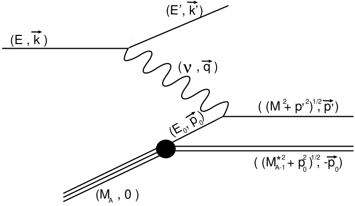
Figure 4.1: PWIA diagram for quasielastic scattering. $E,{\bf k}$ ($E^{\prime},{\bf k^{\prime}}$) are the initial (final) electron energy and momentum. The virtual photon strikes a bound (off-shell) nucleon with energy $E_{0}$ and momentum ${\bf p_{0}}$. The knocked-out nucleon has momentum ${\bf p^{\prime}}={\bf p_{0}}+{\bf q}$ and is on mass shell ($M=M_{nucleon}$). The recoil nucleus has momentum ${\bf-p_{0}}$, and mass $M_{A-1}^{*}$

The inclusive quasielastic cross section can be written as the the exclusive (e,e^′N) cross section integrated over phase space for the ejected nucleon. In the PWIA, the exclusive cross section is just the sum of the cross sections of the individual nucleons:

$${{d^{5}\sigma}\over{dE^{\prime}d\Omega d^{3}\vec{p}^{\prime}}}=\sum_{nucleons}\sigma_{eN}\cdot S^{\prime}_{N}(E_{0},\vec{p}_{0}),$$ (4.1)

where $S^{\prime}_{N}(E_{0},\vec{p}_{0})$ is the spectral function (the probability of finding a nucleon with energy $E_{0}$ and momentum $\vec{p}_{0}$ in the nucleus) and $\sigma_{eN}$ is the electron-nucleon cross section for scattering from a bound (off-shell) nucleon.

Separating the proton and neutron contributions and integrating over the nucleon final state gives us the inclusive cross section:

$${{d^{3}\sigma}\over{dE^{\prime}d\Omega}}=\int{(~{}Z\sigma_{ep}S^{\prime}_{p}(E_{0},\vec{p}_{0})+N\sigma_{en}S^{\prime}_{n}(E_{0},\vec{p}_{0})~{})d^{3}\vec{p}^{\prime}}.$$ (4.2)

We will neglect the difference between the spectral function for protons and neutrons and use $S^{\prime}(E_{0},\vec{p}_{0})$ for all nucleons. In addition, for unpolarized scattering, we will take $S^{\prime}$ to be spherically symmetric. Replacing the proton and neutron spectral functions with $S^{\prime}$ and changing to spherical coordinates, we have:

$${{d^{3}\sigma}\over{dE^{\prime}d\Omega}}=\int{(Z\sigma_{ep}+N\sigma_{en})\cdot S^{\prime}(E_{0},p_{0})\cdot p^{\prime 2}dp^{\prime}d(cos\vartheta)d\varphi},$$ (4.3)

where $\vartheta$ is the angle between the virtual photon and the initial nucleon momentum ($\vec{q}$ and $\vec{p}_{0}$) and $\varphi$ is the angle between the electron scattering plane and the nucleon scattering plane.

Note that $\vec{p}^{\prime}=\vec{p}_{0}+\vec{q}$, and that $\vec{q}$ is fixed by measuring the initial and scattered electron. Therefore, $d^{3}\vec{p}^{\prime}=d^{3}\vec{p}_{0}$. By replacing $p^{\prime 2}dp^{\prime}$ with $p_{0}^{2}dp_{0}$ and noting that S is independent of $\varphi$, we can rewrite the cross section as follows:

$${{d^{3}\sigma}\over{dE^{\prime}d\Omega}}=2\pi\int{\tilde{\sigma}_{0}\cdot S^{\prime}(E_{0},p_{0})\cdot p_{0}^{2}~{}dp_{0}~{}d(cos\vartheta)},$$ (4.4)

where we have defined:

$$\tilde{\sigma}_{0}={1\over{2\pi}}\int_{0}^{2\pi}{(Z\sigma_{ep}+N\sigma_{en})d\varphi}.$$ (4.5)

Noting that the initial and final particles are on-shell, energy conservation gives us the following constraints:

$$M_{A}=E_{0}+\sqrt{M_{A-1}^{*2}+p_{0}^{2}},$$ (4.6)

and

$$M_{A}+\nu=\sqrt{M^{2}+(\vec{p}_{0}+\vec{q})^{2}}+\sqrt{M_{A-1}^{*2}+p_{0}^{2}},$$ (4.7)

where $M_{A}$ is the mass of the initial nucleus, $M_{A-1}^{*}$ is the mass of the recoiling (A-1) system, and M is the mass of the ejected nucleon. Combining these constraints and simplifying gives:

$$E_{0}+\nu=\sqrt{M^{2}+p_{0}^{2}+q^{2}+2\,p_{0}\,q\cos{\vartheta}}.$$ (4.8)

This allows one to determine $E_{0}$ for any value of $\vec{p}_{0}$, given $\nu$ and $\vec{q}$. Therefore, we can rewrite the inclusive cross section from Eq. (4.4) as follows:

$${{d^{3}\sigma}\over{dE^{\prime}d\Omega}}=2\pi\int{\tilde{\sigma}_{0}\cdot S^{\prime}(E_{0},p_{0})\cdot\delta(Arg)\cdot p_{0}^{2}~{}dp_{0}~{}d(cos\vartheta)~{}dE},$$ (4.9)

where $Arg=E_{0}+\nu-(M^{2}+p_{0}^{2}+q^{2}+2\,p_{0}\,q\cos{\vartheta})^{1/2}$.

Using the $\delta$ function to evaluate the $\vartheta$ integral gives:

$${{d^{3}\sigma}\over{dE^{\prime}d\Omega}}=2\pi\int{\tilde{\sigma}_{0}\cdot S^{\prime}(E_{0},p_{0})\cdot{E_{N}\over{p_{0}\,q}}\cdot p_{0}^{2}~{}dp_{0}~{}dE},$$ (4.10)

where $E_{N}$ is to energy of the struck nucleon ($E_{N}=(M^{2}+p^{\prime 2})^{1/2}$).

The spectral function, $S^{\prime}(E_{0},p_{0})$, can be expressed as a function of the separation energy, $E_{s}\equiv M_{A-1}^{*}+M-M_{A}$, rather than as a function of the nucleon’s initial energy. Let us take $S(E_{s},p_{0})\equiv-S^{\prime}(E_{0},p_{0})$, where the Jacobian coming from transforming from $E_{0}$ to $E_{s}$ has been absorbed into the definition of $S$. By taking $\tilde{\sigma}=(E_{N}/q)\cdot\tilde{\sigma_{0}}$ and replacing $S^{\prime}$ with $S$ we can write the cross section (this time with explicit integration limits) as follows:

$${{d^{3}\sigma}\over{dE^{\prime}d\Omega}}=2\pi\int_{E_{s}^{min}}^{E_{s}^{max}}{\int_{p_{0}^{min}(E_{s})}^{p_{0}^{max}(E_{s})}{\tilde{\sigma}\cdot S(E_{s},\vec{p}_{0})\cdot p_{0}~{}dp_{0}~{}dE_{s}}}.$$ (4.11)

The integration limits for $p_{0}$ are the two solutions to the energy conservation condition (Eq. (4.7)) where $\vec{p}_{0}$ is parallel to $\vec{q}$:

$$M_{A}+\nu=\sqrt{M^{2}+y^{2}+2q\,y+q^{2}}+\sqrt{M_{A-1}^{*2}+y^{2}},$$ (4.12)

with $p_{0}^{min}\equiv|y_{1}|$ and $p_{0}^{max}\equiv|y_{2}|$, where $y_{1}$ and $y_{2}$ are the two solutions to the above equation. The minimum separation energy, $E_{s}^{min}$, occurs when the recoil nucleus is the (A-1) ground state. The upper limit, $E_{s}^{max}$, occurs when the struck nucleon is at rest in the final state (where $p_{0}^{min}(E_{s})=p_{0}^{max}(E_{s})$):

$$E_{s}^{max}=\sqrt{(M_{A}+\nu)^{2}-q^{2}}-M_{A}.$$ (4.13)

4.3 $y$-scaling

The scaling limit in the PWIA arises from the behavior of the integration limits in Eq. (4.11) and the form of the cross section and spectral function.

First, we note that the spectral function is expected to be peaked at $p_{0}=0$ and $E_{s}=E_{s}^{0}$ [83], where $E_{s}^{0}$ is the minimum separation energy when the recoil nucleus is in its ground state. As will be seen when we examine the off-shell cross section, $\tilde{\sigma}$ varies extremely slowly with $p_{0}$ and $E_{s}$. The rapid decrease of the spectral function (relative to the slow variation of the cross section) means that it is a good approximation to replace $\tilde{\sigma}(E_{s},p_{0})$ with its value at the peak of the spectral function, $\tilde{\sigma}(E_{s}^{0},p_{0}^{min})$. Finally, we will extend the upper integration limits to infinity. The rapid decrease of the spectral function means that the error made by extending the integration limits will decrease rapidly as $Q^{2}$ increases. By extending the upper limit of integration and replacing $\tilde{\sigma}$ with a constant value, we get the following:

$${{d^{3}\sigma}\over{dE^{\prime}d\Omega}}=2\pi\bar{\sigma}\int_{E_{s}^{min}}^{\infty}{\int_{|y_{1}(E_{s})|}^{\infty}{S(E_{s},p_{0})\cdot p_{0}~{}dp_{0}~{}dE_{s}}},$$ (4.14)

where $\bar{\sigma}=\tilde{\sigma}(E_{s}^{0},p_{0}^{min})$.

Figure 4.2: Integration region of Eq. (4.14) for a variety of kinematics from e89-008. The left figure shows the integration region up to $E_{s}$ of 0.5 GeV/c. The right figure shows the lower $p_{0}$ limits for $E_{s}$ near $E_{s}^{0}$ ($\sim$17 MeV for Carbon). The dotted line is for $\theta=15^{\circ}$, the dashed is $23^{\circ}$, and the solid is $30^{\circ}$.

Finally, we need to look more carefully at the lower limit of the momentum integration, $|y_{1}(E_{s})|$. Figure 4.2 shows the region of integration for scattering from ¹²C for several kinematics measured in the experiment. All contours are for an initial electron energy of 4.045 GeV, with varying angles for the scattered electron. The energy of the scattered electron is chosen so that the contours pass through the point $E_{s}$ = $E_{s}^{0}$ = 0.0173 GeV, $p_{0}$ = 0.15 GeV/c. Because the spectral function is strongly localized within the region of integration, we have already extended the upper integration limits to infinity. Note that as the momentum transfer increases, the lower $p_{0}$ limit becomes a slowly varying and nearly linear function of $E_{s}$. Because the spectral function is localized around $E_{s}=E_{s}^{0}$, we can approximate the lower integration limit with a constant value, $|y_{1}(E_{s})|\approx|y_{1}(E_{s}^{0})|\equiv|y|$. This allows us to rewrite the cross section as:

$${{d^{3}\sigma}\over{dE^{\prime}d\Omega}}=\bar{\sigma}\cdot F(y)$$ (4.15)

where

$$F(y)=2\pi\int_{E_{s}^{min}}^{\infty}{\int_{|y|}^{\infty}{S(E_{s},p_{0})\cdot p_{0}~{}dp_{0}~{}dE_{s}}}$$ (4.16)

is the scaling function.

In order to determine $F(y)$ from the measured cross sections, we need to have the electron-nucleon cross section for an off-shell nucleon. There is no unambiguous procedure for determining the off-shell (e,e^′N) cross section from measurements of the on-shell form factors. For our analysis of the data, we choose the De Forest $\sigma_{1}^{cc}$ prescription [84] for $\sigma_{eN}$:

$$\sigma_{eN}=\frac{\sigma_{m}}{\bar{E}E_{N}}\Biggl{\{}(F_{1}+F_{2})\cdot\Biggl{(}\frac{\bar{Q}^{2}}{2}\tan^{2}{\frac{\theta}{2}}+\frac{Q^{2}}{4q^{2}}(\bar{Q}^{2}-Q^{2})\Biggr{)}+(F_{1}+\frac{\bar{Q}^{2}}{4M^{2}}F_{2})\cdot\Biggr{.}$$

$$\Biggl{.}\Biggl{(}\Biggl{[}\frac{Q^{2}}{2q^{2}}(\bar{E}+E_{N})+\Biggl{(}\frac{Q^{2}}{q^{2}}+\tan^{2}{\frac{\theta}{2}}\Biggr{)}^{1/2}p^{\prime}\sin{\vartheta}\cos{\varphi}\Biggr{]}^{2}+\tan^{2}{\frac{\theta}{2}}p^{\prime 2}\sin^{2}{\vartheta}\sin^{2}{\varphi}\Biggr{)}\Biggr{\}}$$

where $E_{N}=(M^{2}+p^{\prime 2})^{1/2}$, $Q^{2}=q_{\nu}q^{\nu}=q^{2}-\nu^{2}$, $\bar{E}=((\vec{p^{\prime}}-\vec{q})+M^{2})^{1/2}$, and $\bar{q}^{2}=q^{2}-(E_{N}-\bar{E})^{2}$. $\sigma_{m}$ is the Mott cross section, given by:

$$\sigma_{m}=\frac{(\alpha\hbar c)^{2}\cos^{2}{\theta/2}}{4E_{beam}\sin^{4}{\theta/2}}.$$ (4.18)

From this expression we determine the contribution to $\tilde{\sigma}$ from a single nucleon ($\tilde{\sigma}_{N}=\frac{1}{2\pi}\int_{0}^{2\pi}\sigma_{eN}d\varphi$):

$$\tilde{\sigma}_{p(n)}=\frac{\sigma_{m}}{\bar{E}q}\Biggl{\{}(F_{1}+F_{2})\cdot\Biggl{[}\frac{\bar{Q}^{2}}{2}\tan^{2}{\frac{\theta}{2}}+\frac{Q^{2}}{4q^{2}}(\bar{Q}^{2}-Q^{2})\Biggr{]}\;+\Biggr{.}$$ (4.19)

$$\Biggl{.}(F_{1}+\frac{\bar{Q}^{2}}{4M^{2}}F_{2})\cdot\Biggl{[}\frac{Q^{4}}{4q^{4}}(\bar{E}+E_{N})^{2}+\Biggl{(}\frac{Q^{2}}{q^{2}}+\tan^{2}{\frac{\theta}{2}}\Biggr{)}p^{\prime 2}\sin^{2}{\vartheta}\Biggr{]}\Biggr{\}}.$$

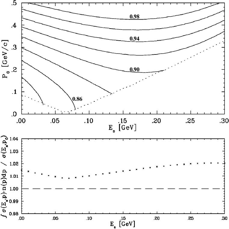
Figure 4.3: The top figure shows $\tilde{\sigma}(E_{s},p_{0})/\tilde{\sigma}(E_{s}^{0},p_{0}^{min})$ contours in the region of integration for Iron at 15^∘, $\nu$=0.6 GeV. The dashed line shows $p_{0}^{min}(E_{s})$. The bottom figure shows the ratio of the cross section weighted by a model momentum distribution to the value of the cross section at the minimum momentum as a function of $E_{s}$.

We obtained scaling in $y$ by assuming that $\tilde{\sigma}$ varied slowly over the integration region. Figures 4.3 and 4.4 show the ratio of $\tilde{\sigma}(E_{s},p_{0})$ to $\tilde{\sigma}_{max}(E_{s},p_{0})$ for two different kinematics. Figure 4.3 is for $\theta$=15^∘, $\nu$=0.6 GeV, and figure 4.4 is for $\theta$=55^∘, $\nu$=2.6 GeV (both are near the top of the quasielastic peak). While this ratio varies by up to $\sim$20%, the average value of $\tilde{\sigma}$ at fixed $E_{s}$, weighted by a model momentum distribution, differs from the value at the minimum momentum by $\mathrel{\raise 1.29167pt\hbox{$<$}\mkern-14.0mu\lower 2.58334pt\hbox{$\sim$}}$2%. The momentum distribution is determined by taking a fit to the measured $F(y)$ and extracting the momentum distribution using equation 4.21. The ratio of $\int\tilde{\sigma}(E_{s},p_{0})n(p)dp$ to $\tilde{\sigma}(E_{s},p_{0}^{min}(E_{s}))$ is shown in the bottom part of figures 4.3 and 4.4 as a function of $E_{s}$.

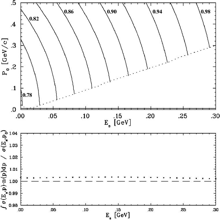
Figure 4.4: The top figure shows $\tilde{\sigma}(E_{s},p_{0})/\tilde{\sigma}(E_{s}^{0},p_{0}^{min})$ contours in the region of integration for Iron at 55^∘, $\nu$=2.6 GeV. The dashed line shows $p_{0}^{min}(E_{s})$. The bottom figure shows the ratio of the cross section weighted by a model momentum distribution to the value of the cross section at the minimum momentum as a function of $E_{s}$.

Once the cross section is measured, and $F(y)$ extracted, we can use the scaling function in order to examine the momentum distribution of the nucleus. $F(y)$ can be expressed in terms of the nucleon momentum distribution, $n(p_{0})$. Because the momentum integration limit no longer depends on $E_{s}$, (once the upper limit is extended to infinity and the lower limit fixed) we can reverse the order of integration, noting that $n(p_{0})=\int_{E_{s}^{min}}^{\infty}{S(E_{s},p_{0})}$, and rewrite $F(y)$ as:

$$F(y)=2\pi\int_{|y|}^{\infty}{n(p_{0})\cdot p_{0}~{}dp_{0}}.$$ (4.20)

We can then express the momentum distribution in terms of the scaling function:

$$n(p_{0})={-1\over{2\pi p_{0}}}{dF(p_{0})\over dp_{0}}.$$ (4.21)

In order to extract the momentum distribution from the scaling function, one needs to verify that the assumptions that lead to the scaling of $F(y)$ are valid. The final-state interactions must be small, the error made by extending the momentum integration limit to infinity must be small, and the region of $E_{s}$ where the spectral function contributes significant strength to the momentum distribution, $n(p_{0})$, must be small enough ( or have a smooth enough $E_{s}$ dependence) that taking the momentum lower limit to be independent of $E_{s}$ is a good approximation. If any of these are not true, then a better model than described here must be used, in order to take into account the final-state interactions or errors made by fixing the integration limits. The data in the scaling region can be used to extract the momentum distribution, but the data showing the approach to scaling is also needed in order to help verify that the assumptions in the model are satisfied, or to demonstrate that the model of final-state interactions used to correct errors coming from the assumptions of the PWIA is adequate.

When the momentum distribution is extracted from the scaling function, it can be used to examine the effects of the nuclear medium, and the nucleon-nucleon interactions. For $|y|<k_{F}$, the Fermi momentum, the momentum distribution is sensitive to the mean field seen by the nucleon in the nucleus. For $|y|>k_{F}$, the momentum distribution is sensitive to short-range correlations of the nucleons. A discussion of the general form of $F(y)$ in terms of the momentum distribution of the nucleons in the nucleus can be found in [78], along with a parameterization for $F(y)$ that takes into account the mean-field and short-range nature of the different regions of the momentum distribution.

In addition to studying the momentum distribution of nucleons in the nucleus, one can look for modifications to the structure of the nucleon when it is in the nuclear medium. It was assumed that the structure function for the nucleon was unchanged when the nucleon was placed inside of a nucleus. If this is not true, then the normalization of the scaling function will be modified. For example, if the size of the nucleon increases when placed in the nucleus, then the form factors at a given $Q^{2}$ would be reduced, and the extracted $F(y)$ would be smaller than expected. In this case, the normalization of $F(y)$ would not agree with it’s definition in terms of the nucleon momentum distribution. Previous data has been used to set limits on the ‘swelling’ of nucleons in the nucleus for ³He [85], and heavier nuclei [34, 86, 87]. However, the previous data on heavy nuclei was at lower $Q^{2}$, where the final-state interactions were still significant. For the data presented here, the final-state interactions may be small enough to examine this problem, but a better model of the inelastic contributions is necessary in order to remove the large inelastic contributions to the data.

4.4 Inelastic Cross Section and $x$-scaling

In the case of inelastic electron scattering, the final state does not consist of a single ejected nucleon and a residual (A-1) nucleus. The struck nucleon can be excited into a resonance state or break up completely. When just the electron is detected in the final state, the only available information about the final state is the invariant mass $W$ of the total hadronic final state:

$$W^{2}=2M\nu+M^{2}-Q^{2}$$ (4.22)

In this case, where the final state is unknown, the PWIA approach used to examine the quasielastic scattering is clearly not applicable. For the general case of unpolarized electron scattering from a charged particle with internal structure, the differential cross section can be written in the one-photon-exchange approximation as:

$$\frac{d^{3}\sigma}{dE^{\prime}d\Omega}=\frac{4\alpha^{2}E^{\prime 2}}{Q^{4}}\left[2W_{1}(\nu,Q^{2})\sin^{2}{\theta/2}+W_{2}(\nu,Q^{2})\cos^{2}(\theta/2)\right].$$ (4.23)

The structure of the system is described by the two unknown functions, $W_{1}$ and $W_{2}$. If we consider the case of inelastic electron-proton scattering, then $W_{1}$ and $W_{2}$ are the structure functions of the proton. As we increase the momentum transfer, the wavelength of the virtual photon will become smaller, and the reaction occurs over a short time scale. If the reaction occurs on a time scale much less than the interaction time of the quarks in the nucleon (the hadronization time), the electron will not ‘see’ the interactions of the quark after the exchange of the virtual photon, and the reaction should look like scattering from a quasi-free quark (bound and off-mass shell, but not interacting with the other quarks). The cross section for elastic scattering from a free structureless, spin-$\frac{1}{2}$ fermion is:

$$\frac{d^{3}\sigma}{dE^{\prime}d\Omega}=\frac{4\alpha^{2}E^{\prime 2}}{Q^{4}}\left[\frac{Q^{2}}{2m_{q}^{2}}\sin^{2}{\theta/2}+\cos^{2}(\theta/2)\right]\frac{1}{\nu}\delta(1-\frac{Q^{2}}{2m_{q}\nu}).$$ (4.24)

We can see that in the high $\nu$ and $Q^{2}$ limit of deep inelastic scattering (DIS), where the scattering is the interaction of the virtual photon with a single quark, the structure functions from Eq. (4.23) take simplified forms. Equating these expressions for the differential cross section and choosing dimensionless versions of the structure functions gives us the following:

$$2m_{q}W_{1}={Q^{2}\over 2m_{q}\nu}\delta(1-{Q^{2}\over 2m_{q}\nu})$$ (4.25)

$$\nu W_{2}=\delta(1-{Q^{2}\over 2m_{q}\nu}).$$ (4.26)

So in the limit where the electron is scattering from a point quark, the structure functions simplify to functions of $\frac{Q^{2}}{2m_{q}\nu}$, rather than functions of $\nu$ and $Q^{2}$ independently. For confined quarks, the $\delta$-function is replaced by the momentum distribution of the quarks. It is conventional to express the structure functions in term of the Bjorken $x$ variable, $x_{Bjorken}={Q^{2}\over 2M\nu}$, where $M$ is the nucleon mass, rather than in terms of $\frac{Q^{2}}{2m_{q}\nu}$. In the limit of $\nu,Q^{2}\rightarrow\infty$ ($\frac{\nu}{Q^{2}}$ finite), $x$ is the fraction of the nucleon’s momentum carried by the struck quark ($0<x<1$), and the structure function in the scaling limit then represents the momentum distribution of the quarks in the nucleon [10]. This can be seen in the parton model of the nucleon. Working in the infinite momentum frame, where the momentum of the nucleon is much larger than the mass of the nucleon, we can assign the struck parton a fraction $\zeta$ of the nucleon’s momentum, energy, and mass. Noting that $\zeta=m_{q}/M$, and so $\frac{Q^{2}}{2m_{q}\nu}=x/\zeta$, Eqs. (4.25 and 4.26) give:

$$F_{1}=MW_{1}=\frac{M}{2m_{q}}{x\over\zeta}\delta(1-{x\over\zeta})=\frac{1}{2\zeta}x\delta(\zeta-x)$$ (4.27)

$$F_{2}=\nu W_{2}=\delta(1-{x\over\zeta})=\zeta\delta(\zeta-x).$$ (4.28)

for the structure function of a single parton. The structure function for the nucleon is just the charge-weighted sum over the individual partons, integrated over the momentum distribution for the partons, $f_{i}(\zeta)$. We can then write $F_{2}$ as:

$$F_{2}^{N}=\sum_{i}\int_{0}^{1}e_{i}^{2}f_{i}(\zeta)F_{2}^{i}(\zeta)d\zeta=\sum_{i}\int_{0}^{1}e_{i}^{2}f_{i}(\zeta)\zeta\delta(\zeta-x)d\zeta=\sum_{i}e_{i}^{2}xf_{i}(x).$$ (4.29)

$F_{1}(x)$ is simply $\frac{x}{2\zeta^{2}}F_{2}(x)$, and so $F_{1}(x)$ and can also be written as a sum over the same parton distribution functions:

$$F_{1}^{N}=\sum_{i}\int_{0}^{1}e_{i}^{2}f_{i}(\zeta)\frac{x}{2\zeta^{2}}F_{2}^{i}(\zeta)d\zeta=\sum_{i}\frac{1}{2}e_{i}^{2}f_{i}(x)=\frac{1}{2x}F_{2}.$$ (4.30)

Thus, the scaling limit of the structure functions is closely related to the momentum distribution of the quarks.

The same argument can be applied to scattering from a nucleus. The expectation of scaling and the connection between the scaling function and the quark momentum distribution holds true for both scattering from a free nucleon, and scattering from a nucleus. In the deep inelastic limit, the structure function for the nucleus should become independent of $Q^{2}$. However, in scattering from a nucleus, the scaling limit of the structure function represents the quark momentum distribution in the nucleus. The quark momentum distribution can be modified from that for a free nucleon by the momentum distribution of the nucleons and by modifications to the internal structure of the nucleon in the nuclear medium. In scattering from a nucleon, $x$ was constrained to be between 0 and 1. In scattering from a nucleus, the nucleons share their momentum, and $x$ can range from 0 to $A$, the number of nucleons in the nucleus.

4.5 $\xi$-scaling

Another variable used to examine scaling in inelastic electron-proton scattering is the Nachtmann variable $\xi=2x/(1+\sqrt{1+\frac{4M^{2}x^{2}}{Q^{2}}})$. As $Q^{2}\rightarrow\infty$, $\xi\rightarrow x$, and so the scaling of the structure function seen in $x$ should also be seen in $\xi$, though the approach to scaling at finite $Q^{2}$ will be different. It was shown by Georgi and Politzer [17] that $\xi$ is the correct variable to use in studying QCD scaling violations in the nucleon. At finite $Q^{2}$, $\xi$ reduces $O(1/Q^{2})$ violations arising from target mass effects which dominate the expected QCD scaling violations. A more recent work by Gurvitz proposes a new scaling variable that includes parton confinement effects [2, 15].

There is also reason to expect scaling in terms of $\xi$ for quasielastic scattering at very high $Q^{2}$. One can expand $\xi$ in terms of $y$:

$$\xi=1-\frac{1}{M}\left[y+\sqrt{M^{2}_{A-1}+y^{2}}-M_{A-1})+E_{s}\right]-\frac{M}{2q}+O(Q^{-2}).$$ (4.31)

Therefore, at very high $Q^{2}$, $\xi$ is a function of $y$, and so for purely quasielastic scattering, the data should show the same type of scaling behavior in $\xi$ as in $y$. However, it will have a different approach to scaling at lower $Q^{2}$ values due to the $\frac{M}{2q}$ and $O(Q^{-2})$ terms. For the $Q^{2}$ range of this experiment and the previous data, the scaling violations due to the $Q^{2}$ dependence of $\xi$ in terms of $y$ are significant, and the scaling behavior seen in terms of $y$ is not expected to be seen as a function of $\xi$.

As with $x$-scaling, $\xi$-scaling should also be valid for scattering from a nucleus, as long as we look in the deep inelastic limit. In addition, one might expect to see some kind of scaling behavior in the quasielastic region, but not for the $Q^{2}$ values measured in the previous data. However, in addition to reducing the scaling violations in deep inelastic scattering, $\xi$ also appears to extend the scaling into the resonance and quasielastic regions in previous data [35], where the $x$-scaling picture of scattering from a quasi-free quark is not valid.

For purely inelastic scattering, the data are expected to show scaling in $\xi$, similar to the $x$-scaling. It was observed [35] (figure 1.7) that in electron scattering from nuclei the structure function, $\nu W_{2}$, appeared to scale at the largest measured values of $Q^{2}$ for all values of $\xi$, not just for low $\xi$ (corresponding to DIS) or high $\xi$ (QE). The onset of scaling occurred at higher $Q^{2}$ values as $\xi$ increased, but there were indications of scaling behavior for all $\xi$. Figures 1.6 and 1.7 show the measured structure function for Iron plotted against $x$ and $\xi$. The data scales in $x$ only at the lowest values of $x$ ($x\mathrel{\raise 1.29167pt\hbox{$<$}\mkern-14.0mu\lower 2.58334pt\hbox{$\sim$}}0.4$), far into the inelastic region. But when taken vs. $\xi$, the structure function appears to be approaching a universal curve for all values of $\xi$.

It has been suggested [35] that this observed scaling is a consequence of the local duality observed by Bloom and Gilman [20] in electron-proton scattering. Examining the structure function in the resonance region as a function of $\omega^{\prime}=1/x+M^{2}/Q^{2}$ and $Q^{2}$, they observed that the resonance form factors have the same $Q^{2}$ behavior as the structure functions, and that the scaling limit of the inelastic structure functions could be generated by (locally) averaging over the resonance peaks seen at low $Q^{2}$. The strengths of the resonances (at fixed $W^{2}$) fall more rapidly with $Q^{2}$ than the inelastic structure function (at fixed $\omega^{\prime}$, which corresponds to fixed $x$ at high $Q^{2}$ where $\omega^{\prime}\approx 1/x$). However, as $Q^{2}$ increases, the resonances shift to lower values of $\omega^{\prime}$, and because the structure function falls as $\omega^{\prime}$ decreases, the resonance peaks maintain a constant strength with respect to the inelastic structure function (see figure 1.3). When examined as a function of $x$ instead of $\omega^{\prime}$, the elastic peak is fixed at $x=1$, and therefore does not exhibit this local duality. It was later shown [23] that this duality was predicted by perturbative QCD, and that it includes the elastic peak if the structure function is taken as a function of $\xi$. More recently, West showed that the duality relation:

$$\frac{2M}{Q^{2}}\int_{0}^{\bar{\nu}}d\nu F_{2}(\nu,Q^{2})=\int_{1}^{\bar{\omega}^{\prime}}d\omega^{\prime}F_{2}(\omega^{\prime}),$$ (4.32)

is valid near $x=1$ [88].

If this same behavior is true for a nucleon in the nucleus, then the momentum distribution of the nucleons may cause this averaging of the resonances and the elastic peak. If this is the case, then we would expect the $\xi$-scaling of the deep inelastic structure function to extend into the resonance region, since the resonances, averaged locally by the nucleus, will have the same $Q^{2}$ behavior as the DIS structure function. If the local duality is unaffected by the nuclear medium, and if the nucleon momentum provides appropriate averaging over the resonances, then we might expect duality to hold for all values of $\xi$. This would allow extraction of the scaling limit of the structure function from data at moderate $Q^{2}$, even in the presence of resonance or quasielastic contributions. Bloom-Gilman duality has been examined in nuclei [89], and new, high-precision measurements have been made at CEBAF to study duality on the proton, neutron, and deuteron [90]. There are also approved experiments [91, 92] that will look for duality in the spin structure functions, and use Bloom-Gilman duality to measure higher-twist effects.

An alternative explanation has been proposed by by Benhar and Luiti [37]. They explain the observed scaling at high $\xi$ values in terms of the $y$-scaling of the quasielastic cross section. They suggest that the $Q^{2}$ dependence that arises from examining $\xi$ rather than $y$ is cancelled by the $Q^{2}$ dependence of the final-state interactions. They predict that this cancellation will lead to an ‘accidental’ scaling of the structure function, and that the scaling violations seen in the previous data should continue up to higher $Q^{2}$ values. This will be discussed in more detail in section 5.8.

4.6 Final-State Interactions

For both quasielastic and deep inelastic scattering, a scaling behavior is expected in the limit of large momentum transfers. The argument for scaling in both cases relies in part on the assumption that the final-state interactions will become small as the momentum transfer increases, and that the electron will exchange a photon with a single particle (nucleon or quark), which is bound, but which momentarily behaves as if it’s not interacting with the rest of the nucleus (over the time scale of the interaction with the virtual photon). Because the electromagnetic interaction is relatively weak, it is well described by the exchange of a single virtual photon, and it is assumed that the virtual photon does not interact with the residual nucleus. A more significant final-state interaction comes from the struck object (nucleon or quark) interacting with the rest of the nucleus. These final-state interactions can be quite large, and in some cases are the dominant contribution to the measured cross section.

In a simple picture, these final-state interactions (FSIs) are expected to decrease rapidly as the energy and momentum transfers increase. In the parton model, the FSIs are assumed to be higher-twist effects, and therefore fall at least as quickly as $m^{2}/Q^{2}$. This assumption is based on the fact that as the energy of the virtual photon increases, the interaction time between the photon and struck object decreases. If this interaction time is significantly smaller than the interaction time between the struck object and the rest of the nucleus, then the inclusive scattering should be largely unaffected by the FSIs of the struck nucleon or quark.

There have been several attempts to check this assumption in non-relativistic two-body models [3, 4, 5, 6, 7, 93], and more recently in relativistic models [2, 8]. These models indicate that the effects of final-state interactions are in agreement with the parton model assumptions. In addition, the observation of $y$-scaling behavior in previous data [24, 29, 94, 95, 96] indicate that the final state interactions are becoming small at moderate $Q^{2}$ values ($Q^{2}>$ 2-3 (GeV/c)²).

However, it has recently been argued that the final state interactions in quasielastic scattering may not fall as rapidly as expected from the parton model. In ref. [77], the authors consider absorption of the virtual photon by a pair of correlated nucleons. They conclude that for $1.3\mathrel{\raise 1.29167pt\hbox{$<$}\mkern-14.0mu\lower 2.58334pt\hbox{$\sim$}}x\mathrel{\raise 1.29167pt\hbox{$<$}\mkern-14.0mu\lower 2.58334pt\hbox{$\sim$}}2$, the cross section has a large contribution from the interaction of the virtual photon with a correlated pair, and the rescattering of the pair into the continuum. Figure 4.5 shows their calculation of final-state interactions broken up into mean field and correlated pair contributions. The contributions from the correlated nucleons are still large even at $Q^{2}=3.0$ GeV/c, and show little $Q^{2}$ dependence. The fact that the final-state interactions are nearly $Q^{2}$ independent above $Q^{2}$=2-3 (GeV/c)² could lead to the observed scaling behavior even though the final-state interactions are still large, and the assumptions of the PWIA are not satisfied.

Figure 4.5: Final-state interactions in Iron from correlated nucleons at $x>1$ (from [77]). The dotted line represents the Impulse Approximation contribution to $F(y)$, the dot-dashed line represents the mean field contributions to the final-state interactions, the dashed line shows the final-state interactions from correlated nucleons pairs, and the solid line represents the full calculation (Impulse Approximation + full final-state interactions). The data are from the NE3 measurement.

While the observations of scaling behavior is not sufficient to rule out the possibility of large final-state interactions, the normalization of the scaling function $F(y)$ may be able to limit the size of possible final-state interactions. In the absence of final-state interactions, $F(y)$ was shown to be closely related to the momentum distribution of the nucleons in the nucleus. By measuring the scaling function over a range of $Q^{2}$ values, the models for the final-state interactions can be tested, both in the region where they fall rapidly, and in the regions where the data show scaling, and the FSIs appear to be small. In addition, a careful extraction of the momentum distribution from the scaling function can be used to constrain the size of the final state interactions based on the normalization condition for the momentum distribution. However, if the final-state interactions are large relative to the elementary cross section only in the tails of the momentum distribution, then the normalization of the momentum distribution will not be sensitive to the presence of final-state interactions.

Chapter 5 Results

5.1 Measured Cross Sections

Figures (5.1) through (5.3) show the cross sections for all of the solid targets. The cross sections have had the radiative effects removed, and are corrected for all dead times and inefficiencies. The error bars shown are statistical only. The systematic uncertainties in the cross section are listed in table 3.7. It was decided to delay the analysis of the deuterium data, due to early problems in understanding the spectrometer acceptances. These problems were worse for the extended targets, and so the initial analysis focussed on the solid targets. During the course of the analysis, the acceptance problems were resolved, and the deuterium data will be available in the near future.

Figure 5.1: Carbon cross sections. Errors shown are statistical only. The $Q^{2}$ values indicated are for $x=1$.

Figure 5.2: Iron cross sections. Errors shown are statistical only. The $Q^{2}$ values indicated are for $x=1$.

Figure 5.3: Gold Cross Sections. Errors shown are statistical only. The $Q^{2}$ values indicated are for $x=1$.

Figure 5.4 shows the cross section for iron, compared to calculations provided by Rinat [97, 98] and Simula [76, 77]. The dashed line is the prediction by Rinat and Taragin. Their calculation is based on a convolution of the free nucleon structure function with a structure function for a nucleus composed of point particles. It is argued to be valid for large $Q^{2}$, but shows significant discrepancies for the lowest angles ($Q^{2}\mathrel{\raise 1.29167pt\hbox{$<$}\mkern-14.0mu\lower 2.58334pt\hbox{$\sim$}}2$). Their prediction is high for the low energy loss values at each angle, but is very sensitive to the tails of the momentum distribution used in extracting their point-nucleon structure function. The calculation shown is for their $n_{2}$ momentum distribution [99]. The cross section calculated for extremely low $\nu$ (e.g. $\nu\mathrel{\raise 1.29167pt\hbox{$<$}\mkern-14.0mu\lower 2.58334pt\hbox{$\sim$}}1.0$ at 30^∘) can be significantly lower (by a factor of 2-5) for their $n_{1}$ and $n_{3}$ momentum distributions. In addition, uncertainties in the final-state interactions in this region can be large. The solid line is the calculation by Ciofi degli Atti and Simula. This calculation used the convolution approach of Refs. [100, 101], using the nucleon spectral function of Refs. [102, 103] to calculate the inelastic contributions, and the method of Ref. [77] to calculate the quasielastic contributions and final-state interactions. In addition to final-state interactions from single nucleon rescattering (interactions of a single nucleon knocked out of a shell model state), the authors include final-state interactions for two-nucleon rescattering, where the virtual photon interacts with a correlated pair of nucleons. For $1.3\mathrel{\raise 1.29167pt\hbox{$<$}\mkern-14.0mu\lower 2.58334pt\hbox{$\sim$}}x\mathrel{\raise 1.29167pt\hbox{$<$}\mkern-14.0mu\lower 2.58334pt\hbox{$\sim$}}2$, the final-state interactions are dominated by the interaction of the virtual photon with a correlated pair, and the rescattering of the pair into the continuum. At low $\nu$, corresponding to large values of the initial nucleon momentum, uncertainty in the high-momentum portion of the spectral function leads to an uncertainty in the calculated cross section.

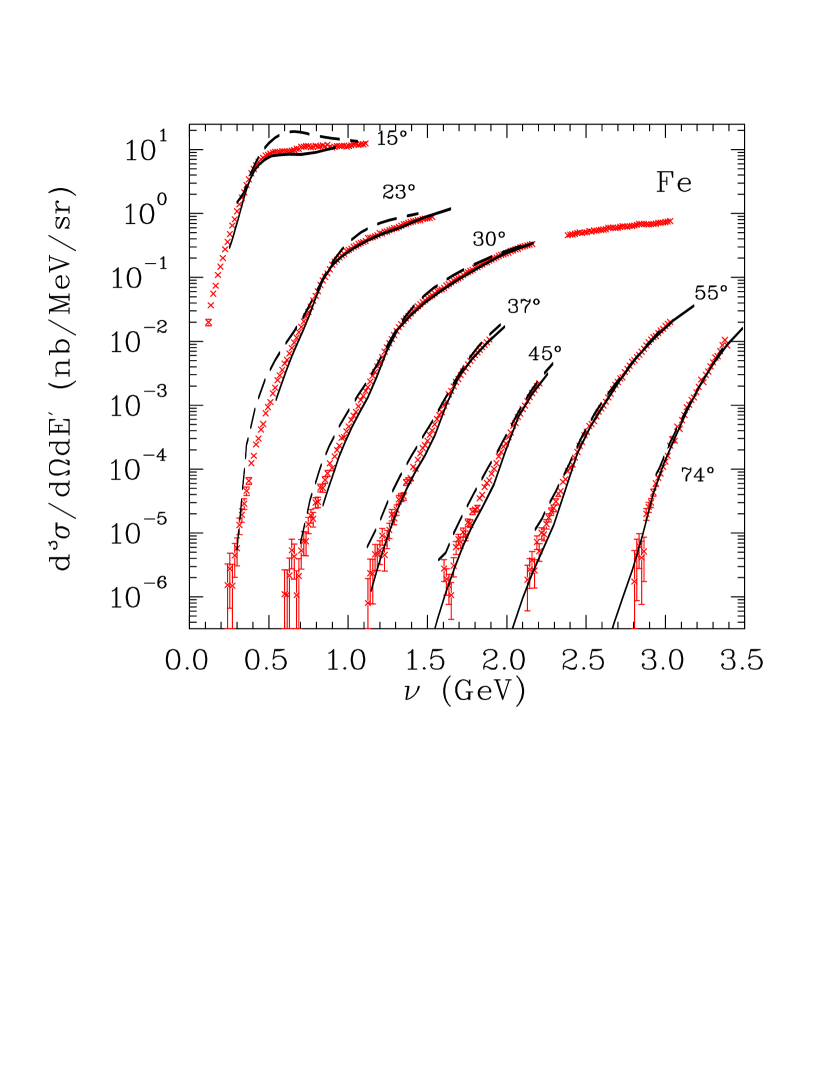
Figure 5.4: Measured Iron cross section compared to theoretical predictions by Rinat and Taragin [97, 98] (dashed lines) and Ciofi degli Atti and Simula [77] (solid lines). The prediction by Rinat and Taragin is not expected to be valid for low $Q^{2}$ values, and shows a noticeable difference from the data at the lowest angles. Both calculations are sensitive to the high momentum components of the assumed momentum distribution or spectral function used in the calculation.

5.2 Extraction of $F(y)$

In order to derive the scaling function $F(y)$ from the cross section, we solve Eq. (4.15) for $F(y)$:

$$F(y)=\frac{d^{3}\sigma}{dE^{\prime}d\Omega}\cdot\bar{\sigma}^{-1}$$ (5.1)

where $\bar{\sigma}$ uses the off-shell cross section from Eq. (4.3) and the values of $E_{s}^{0}$ in table 5.1, with $y$ calculated using Eq. (4.12). The values of $E_{s}^{0}$ are the mass differences between the initial and final (A-1) nuclei, averaged between proton and neutron knock-out and weighted by isotopic abundance of the targets. Note that the values of $E_{s}^{0}$ used in this analysis differ from the values used in analyzing the NE3 and NE18 SLAC data [24, 34, 25], but are consistent with the definition of Pace and Salmè [12]. $F(y)$ for the SLAC data presented here have been recalculated using the values of $E_{s}^{0}$ from table 5.1.

Nucleus	$E_{s}^{0}$ (MeV)
2H	2.25
C	17.27
Fe	10.60
Au	6.93

Table 5.1: $E_{s}^{0}$ values used to determine $y$.

5.3 $y$-scaling

The measured scaling functions are expected to converge to the scaling limit as $Q^{2}$ increases. In the absence of final-state interactions, $F(y)$ should approach the scaling limit from below as the integration region in Eq. (4.11) increases, and the approximation of extending the upper limits to infinity becomes better. Final-state interactions can change this picture significantly. In addition, at positive $y$ values, there is a large deep inelastic contribution to the scattering, which increases as the momentum transfer increases. For values of $Q^{2}$ above $\sim$1-2 (GeV/c)², these contributions become significant even for negative $y$ values, causing the scaling to break down at high $Q^{2}$, even for values of $y$ near $-250$ MeV/c.

Figures (5.5) through (5.7) show $F(y)$ vs. $y$ for Carbon, Iron, and Gold. The error bars shown are statistical only. The fractional systematic uncertainties are identical to the uncertainties given for the cross section in table 3.7. For purely quasielastic scattering, $F(y)$ should be symmetric about $y=0$, and should show scaling for all $Q^{2}$ values high enough that the assumptions in our PWIA model are valid. The inelastic scattering contributes significant strength at $y>0$, and the contribution of the inelastic scattering increases relative to the quasielastic data as $Q^{2}$ increases. Therefore, $F(y)$ is asymmetric, and increases with $Q^{2}$ for $y\mathrel{\raise 1.29167pt\hbox{$>$}\mkern-14.0mu\lower 2.58334pt\hbox{$\sim$}}0$. For $y\mathrel{\raise 1.29167pt\hbox{$<$}\mkern-14.0mu\lower 2.58334pt\hbox{$\sim$}}-0.3$ GeV, the inelastic contributions are small, and we see the behavior of the quasielastic contribution. In the derivation of $y$-scaling, we extended the integration limits of the nucleon initial momentum to infinity. As $Q^{2}$ increases, this approximation should become better, and the measured $F(y)$ should approach the scaling limit from below, as more of the spectral function is included in the integration. However, final state interactions are the dominant source of scale-breaking for low momentum transfers, and the data approach the scaling limit from above.

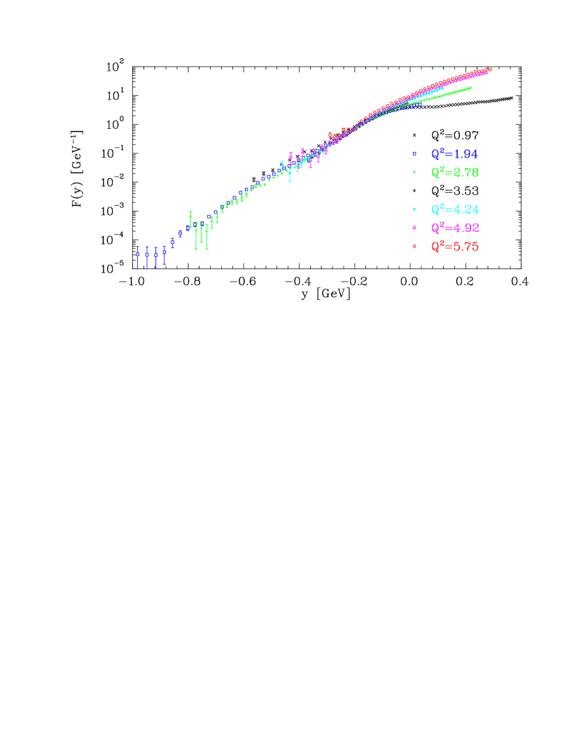
Figure 5.5: $F(y)$ for Carbon. Errors shown are statistical only. The $Q^{2}$ values indicated are for $x=1$.

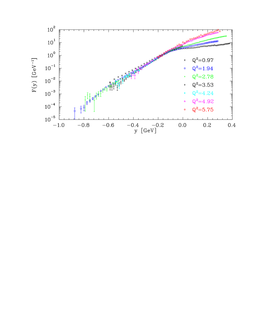
Figure 5.6: $F(y)$ for Iron. Errors shown are statistical only. The $Q^{2}$ values indicated are for $x=1$.

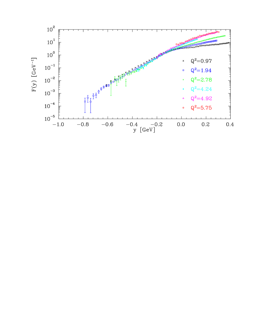
Figure 5.7: $F(y)$ for Gold. Errors shown are statistical only. The $Q^{2}$ values indicated are for $x=1$.

Figures 5.8 and 5.9 shows the approach to scaling for several values of $y$ for Iron. The e89-008 data is shown along with the NE3 [34] data, for which $y$ has been recalculated using the the same $E_{s}^{0}$ values used for e89-008. The lines are the calculations by Simula [76, 77], with the quasielastic contribution shown with a dotted line, and the total shown with a solid line. For low values of $|y|$, there is a clear breakdown of scaling for the high $Q^{2}$ values due to the contribution from inelastic scattering. For higher $|y|$, the data are independent of $Q^{2}$. In the vicinity of $y=-0.3$, the calculation underestimates the data. Figure 5.10 shows the data versus the calculation as a function of $y$ at 30^∘ and 45^∘. The calculation shows a dip in the scaling function near $y=-0.3$ GeV/c for all $Q^{2}$ values, and somewhat underestimates $F(y)$ for more negative values of $y$. For large values of $y$, there are significant uncertainties coming from uncertainties in the calculation of the final state interactions, and from uncertainties in the spectral function at very large momenta (above the Fermi momentum).

Figure 5.8: Approach to scaling of $F(y)$ for Iron. $F(y)$ values at fixed $y$ are interpolated from the data and shown vs. $Q^{2}$ for several values of $y$. Solid symbols are e89-008 data, and hollow symbols are data from NE3 (and NE18 for $y=0$). The lines are the calculation by Simula. The dashed line is the quasielastic contribution and the solid line is the total.

Figure 5.9: Approach to scaling of $F(y)$ for Iron. $F(y)$ values at fixed $y$ are interpolated from the data and shown vs. $Q^{2}$ for several values of $y$. Solid symbols are e89-008 data, and hollow symbols are data from NE3. The lines are the calculation by Simula. The dashed line is the quasielastic contribution and the solid line is the total.

Figure 5.10: $F(y)$ versus $y$ for Iron at 30^∘ and 45^∘. The data are shown along with the calculation by Simula for the quasielastic contribution (dashed line) and total (QE+DIS) contribution (solid line).

5.4 Subtraction of the Inelastic Background.

If we wish to use the measurement of $F(y)$ to examine the momentum distribution of the nucleons, we need to extract $F(y)$ for all values of $y$, in a region where the effects of final-state interactions are small. Because $F(y)$ is symmetric about $y=0$, we only need to extract the scaling function for $y<0$. While the final-state interactions are smaller at higher momentum transfer (though not necessarily negligible), the inelastic cross section begins to become important for small values of $|y|$ as we go to higher $Q^{2}$. In order to try to disentangle the quasielastic and inelastic contributions, we will use a model of the inelastic cross section to subtract the inelastic contributions.

5.4.1 Inelastic Subtracted $F(y)$.

Figures (5.11) through (5.13) show the background subtracted $F(y)$ vs. $y$ for Carbon, Iron, and Gold. The error bars shown are statistical only. The model of the inelastic contributions is described in section 3.4.1. It is a modified version of the convolution procedure of Benhar, et al. [69], but has been extended to lower $Q^{2}$ values than it was designed for, and been modified to match our data in the DIS region. For the $Q^{2}$ values measured, a full convolution of the spectral function with the cross section would be a better approach, but this model was chosen because it is significantly faster to compute, and in the radiative correction procedure, the computation time was a significant factor.

In the region of $y\mathrel{\raise 1.29167pt\hbox{$>$}\mkern-14.0mu\lower 2.58334pt\hbox{$\sim$}}-0.1$ GeV, subtracting the inelastic contribution significantly reduces the scaling violations at larger $Q^{2}$, as expected. The scaling function now decreases for positive $y$, and is roughly symmetric about $y=0$ for small $|y|$. However, for the largest values of $y$, the inelastic contributions can be 10-1000 times larger than the quasielastic contributions. Therefore, while the model can be compared to the cross section at low $x$ (large positive $y$) in order to check the normalization of the model, a small error in the model can lead to an error much larger than the extracted value of $F(y)$. While the uncertainty in the inelastic model at negative values of $y$ is fairly large, the inelastic contributions in this region are generally quite small. Only for values near $y=0$ does this uncertainty have a significant impact on the subtracted values at high $Q^{2}$. A better model is required in order to have a good measurement of $F(y)$ for small values of $|y|$, which is an important region in checking the normalization of $F(y)$.

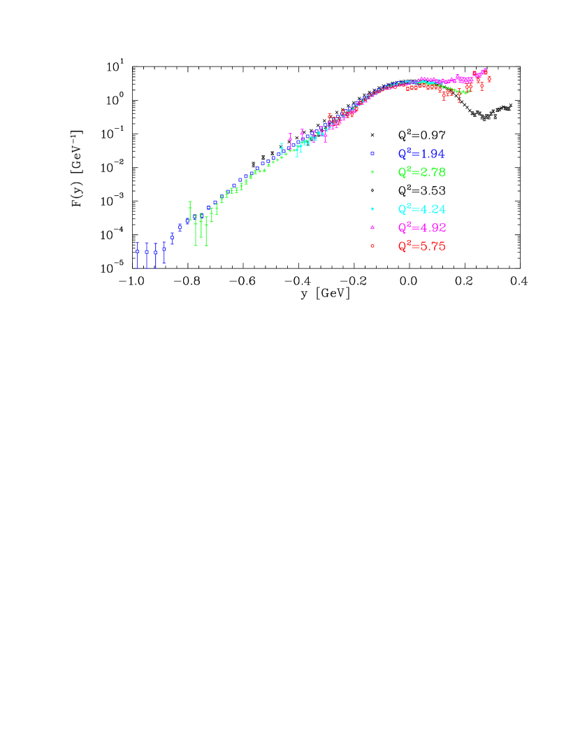
Figure 5.11: Background subtracted $F(y)$ for Carbon. Errors shown are statistical only. The $Q^{2}$ values indicated are for $x=1$.

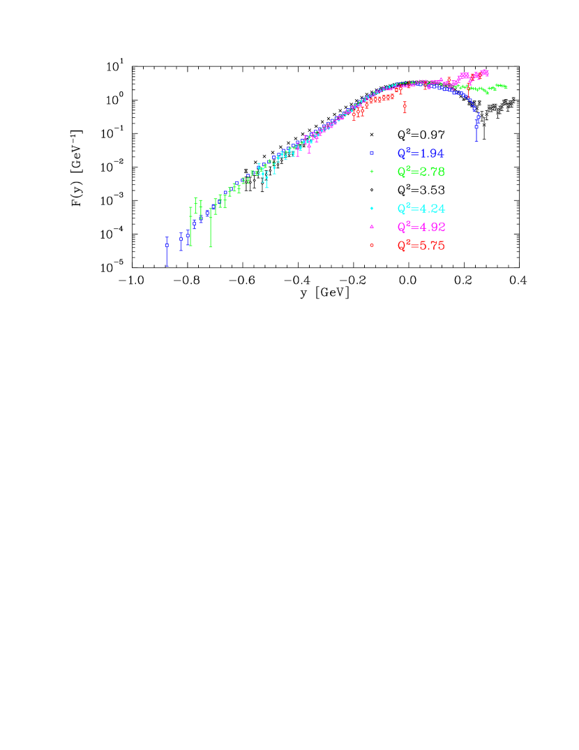
Figure 5.12: Background subtracted $F(y)$ for Iron. Errors shown are statistical only. The $Q^{2}$ values indicated are for $x=1$.

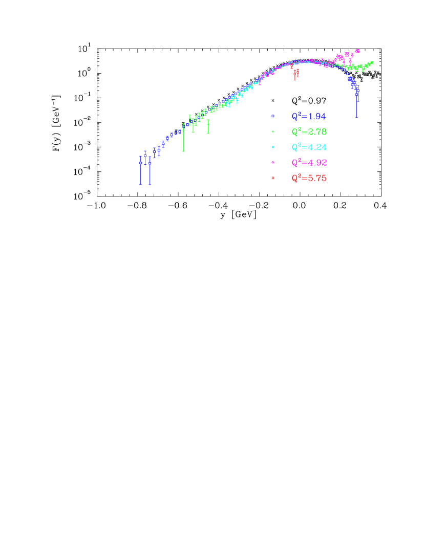
Figure 5.13: Background subtracted $F(y)$ for Gold. Errors shown are statistical only. The $Q^{2}$ values indicated are for $x=1$.

5.5 Alternate $y$-scaling Variables.

There are alternative scaling variables and scaling functions that can be used to examine scaling of the quasielastic cross section. Some of these come about from modifying the assumptions used in reducing the PWIA cross section to the scaling limit. For example, in section 4.3 we chose to replace the off-shell cross section with it’s value at $E_{s}^{0}$, the minimum separation energy with the recoil nucleus in the ground state. In the analysis of the SLAC NE3 data [34], the cross section was taken at a value of $E_{s}$ based on measurements of the spectral function for a variety of nuclei [104] and corrected to compensate for the relativistic recoil of the nucleon. While the difference in choice of $E_{s}^{0}$ does not modify the conclusion that $F(y)$ will show scaling at large $Q^{2}$, it does modify the exact form of the scaling function, and in particular the approach to scaling at lower $Q^{2}$.

In addition, other scaling functions have been suggested for examining the quasielastic scattering. A modified scaling was proposed by Sick, Day, and McCarthy [95]. In their approach, the scaling variable $y^{\prime}$ is obtained from:

$$\omega=(m^{2}+Q^{2}+2Qy^{\prime}+y{{}^{\prime}2}+k_{\perp}^{2})^{1/2}+(y^{\prime 2}+((A-1)m)^{2})^{1/2}-Am+E_{s}$$ (5.2)

where $k_{\perp}=\sqrt{0.4}k_{F}$. The scaling function is defined as:

$$F_{2}(y^{\prime})=\frac{d^{2}\sigma}{d\Omega dE^{\prime}}\frac{1}{(Z\sigma_{ep}+N\sigma_{en})}\frac{\partial\omega}{\partial y^{\prime}}.$$ (5.3)

More recently, a modified version of the $y$-scaling variable was proposed [78] that is designed to represent the two-nucleon correlation tail at large values of $y$. This is done by calculating $y$ assuming that the final state consists of the knocked out nucleon, a correlated nucleon with momentum opposite to the initial momentum of the knocked out nucleon, and a recoiling ($A$-2) spectator system in an unexcited state (as shown in figure 5.14). For these assumptions, the new scaling variable, $y_{2}$, is given by:

$$y_{2}=\left|-\frac{q}{2}+\left[\frac{q^{2}}{4}-\frac{4\tilde{\nu}^{2}M^{2}-\tilde{W}^{4}}{\tilde{W}^{2}}\right]^{1/2}\right|,$$ (5.4)

where $\tilde{\nu}=\nu+\tilde{M}$, $\tilde{M}=2M-E_{th}^{(2)}$, $E_{th}^{(2)}=\left|E_{A}\right|-\left|E_{A-2}\right|$, and $\tilde{W}^{2}=\tilde{M}^{2}+2\nu\tilde{M}-Q^{2}$. $y_{2}$ can be interpreted as the scaling variable related to a deuteron-like configuration within the nucleus, with mass $\tilde{M}=2M-E_{th}^{(2)}$. $y_{2}$ is designed to take into account the nature of the correlations for large $|y|$, and reduce the uncertainties in the extraction of the momentum distribution by reducing the binding corrections that have to be made in order to account for the error made by taking a fixed $E_{s}$ (i.e. assuming that the residual (A-1) nucleus is in it’s ground state). It should therefore improve scaling in the correlation region, but for small values of $y_{2}$, $y_{2}\approx y$. Therefore, $y_{2}$ is useful over the entire region of $y$.

Additional scaling variables similar to $y$ are discussed in [13].

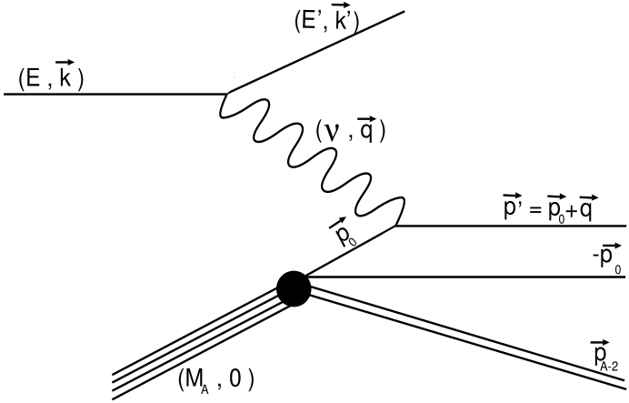
Figure 5.14: PWIA diagram for quasielastic scattering with a correlated pair of nucleons. $E,{\bf k}$ ($E^{\prime},{\bf k^{\prime}}$) are the initial (final) electron energy and momentum. The virtual photon strikes a bound (off-shell) nucleon with energy $E_{0}$ and momentum ${\bf p_{0}}$. The struck nucleon is part of a deuteron-like configuration within the nucleus, and there is a spectator nucleon with momentum ${-\bf p_{0}}$. The knocked-out nucleon has momentum ${\bf p^{\prime}}={\bf p_{0}}+{\bf q}$ and is on mass shell ($M=M_{nucleon}$). The recoil nucleus has a recoil momentum ${\bf p_{A-2}}$, and mass $M_{A-2}$

5.6 Extraction of the Structure Function

The inclusive differential cross section from Eq. (4.23) can be written in the following form:

$$\frac{d^{\sigma}}{d\Omega dE^{\prime}}=\sigma_{Mott}\left[W_{2}+2W_{1}\tan^{2}(\theta/2)\right],$$ (5.5)

where $\sigma_{Mott}=4\alpha^{2}E^{2}\cos^{2}(\theta/2)/Q^{4}$. In order to separate the structure functions $W_{1}$ and $W_{2}$ we would need a measurement of the $\theta$ dependence of the cross section at fixed $\nu$ and $Q^{2}$. Because we have not measured this, we need to make an assumption about the ratio of the transverse to the longitudinal cross section, $R=\sigma_{L}/\sigma_{T}=(1+\nu^{2}/Q^{2})W_{2}/W_{1}-1$. Given a value for $R$, we can determine the dimensionless structure function $\nu W_{2}$ directly from the cross section:

$$\nu W_{2}=\frac{\nu}{1+\beta}\cdot\frac{\frac{d\sigma}{d\Omega dE^{\prime}}}{\sigma_{Mott}},$$ (5.6)

where

$$\beta=2\tan^{2}(\theta/2)\frac{1+\frac{Q^{2}}{4M^{2}x^{2}}}{1+R}=2\tan^{2}(\theta/2)\frac{1+\frac{\nu^{2}}{Q^{2}}}{1+R}.$$ (5.7)

Because we do not directly measure $R$ in this experiment, we must assume a value for $R$ and assign additional uncertainty in the extracted value of the structure function based on the uncertainty in our knowledge of $R$. Fortunately, the large uncertainty in $R$ has a relatively small effect on the uncertainty in $\nu W_{2}$. For small scattering angles, the contribution from $W_{1}$ is suppressed by a factor of $\tan^{2}(\theta/2)$. The uncertainty associated with $R$ increases for larger angles.

In the quasielastic region, $R$ for an isoscaler target can be expressed in terms of the elastic nucleon form factors in the non-relativistic plane-wave impulse approximation [105]:

$$R=\frac{4M^{2}(G_{Ep}^{2}+G_{En}^{2})}{Q^{2}(G_{Mp}^{2}+G_{Mn}^{2})}.$$ (5.8)

Assuming scaling for the nucleon elastic form factors, $G_{Ep}(Q^{2})=G_{Mp}(Q^{2})/\mu_{p}=G_{Mn}(Q^{2})/\mu_{n}$, and $G_{En}=0$, $R$ becomes:

$$R=\frac{4M^{2}}{Q^{2}(\mu_{p}^{2}+\mu_{n}^{2})}=\frac{0.32\mbox{(GeV/c)}^{2}}{Q^{2}}.$$ (5.9)

A measurement of $R$ near $x=1$ in a $Q^{2}$ range identical to e89-008 [36] indicates that R is independent of $x$, and is well described by $R=0.32/Q^{2}$, though with large uncertainties for $Q^{2}$ values above 4 (GeV/c)². In the deep inelastic range, data taken in a $Q^{2}$ range from 1-5 (GeV/c)² and for $0.2<x<0.5$ [106, 107, 108], indicate that $R$ for Iron in the DIS region is less than 0.5, and has little dependence on $x$ or on the target mass. The data are fairly well described by $R=0.5/Q^{2}$. For our analysis, we assume $R=0.32/Q^{2}$, with a 100% uncertainty in R. This give a maximum uncertainty in $\nu W_{2}$ of $\sim$6% for the largest energy transfer at $74^{\circ}$. At this angle, the systematics in the cross section are dominated by the uncertainty in the subtraction of the charge-symmetric background, and are larger than the uncertainty due to $R$. For the angles below $74^{\circ}$, the uncertainty due to $R$ varies from 0.5% to 5.0%, and is largest at the larger angles (as shown in figure 3.39).

5.7 $x$-scaling

Figures (5.15) through (5.17) show $\nu W_{2}(x,Q^{2})$ vs. $x$ for Carbon, Iron, and Gold. The error bars shown are statistical only. The systematic uncertainties are identical to the uncertainties given for the cross section in table 3.7 except for the additional uncertainty caused by the uncertainty in $R$.

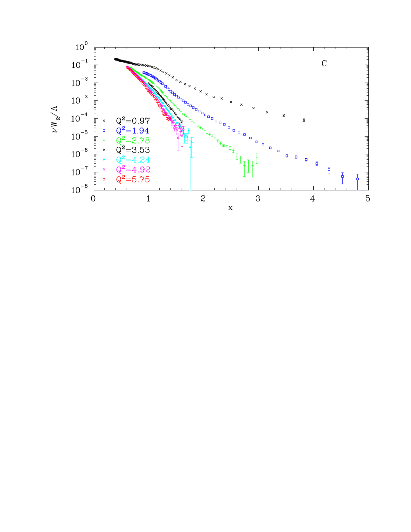
Figure 5.15: Carbon structure function, $\nu W_{2}^{C}(x,Q^{2})$. Errors shown are statistical only. The $Q^{2}$ values indicated are for $x=1$.

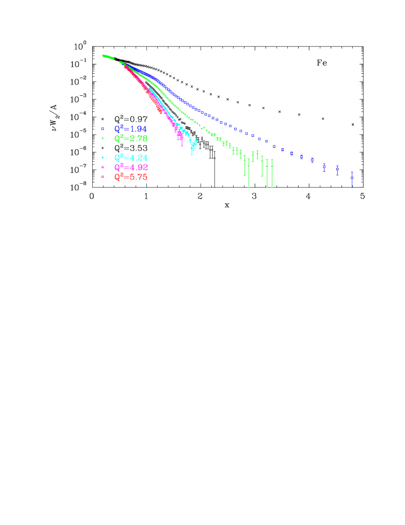
Figure 5.16: Iron structure function, $\nu W_{2}^{Fe}(x,Q^{2})$. Errors shown are statistical only. The $Q^{2}$ values indicated are for $x=1$.

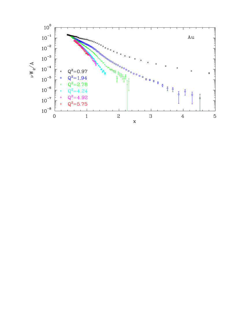
Figure 5.17: Gold structure function, $\nu W_{2}^{Au}(x,Q^{2})$. Errors shown are statistical only. The $Q^{2}$ values indicated are for $x=1$.

For all of the target nuclei, it is clear that $x$-scaling is not valid for this range of $Q^{2}$ except at the lowest $x$ values measured ($x\mathrel{\raise 1.29167pt\hbox{$<$}\mkern-14.0mu\lower 2.58334pt\hbox{$\sim$}}0.5$). At low $x$ values, the dominant process is deep inelastic scattering. In this region, we see the expected $x$-scaling, and the structure function at fixed $x$ becomes independent of $Q^{2}$. As $x$ increases, quasielastic contributions become more important, and the scaling is violated due to the $Q^{2}$ dependence of the nucleon elastic form factors. The success of $y$-scaling in the region $y<0$ (corresponding to $x\mathrel{\raise 1.29167pt\hbox{$>$}\mkern-14.0mu\lower 2.58334pt\hbox{$\sim$}}1$) indicates that for large $x$ values, the process is dominated by quasielastic scattering, and we should not expect to see scaling of the structure function.

5.8 $\xi$-scaling

Figures (5.18) through (5.20) show $\nu W_{2}$ for Carbon, Iron, and Gold, but this time as a function of $\xi$ and $Q^{2}$. The error bars shown are statistical only.

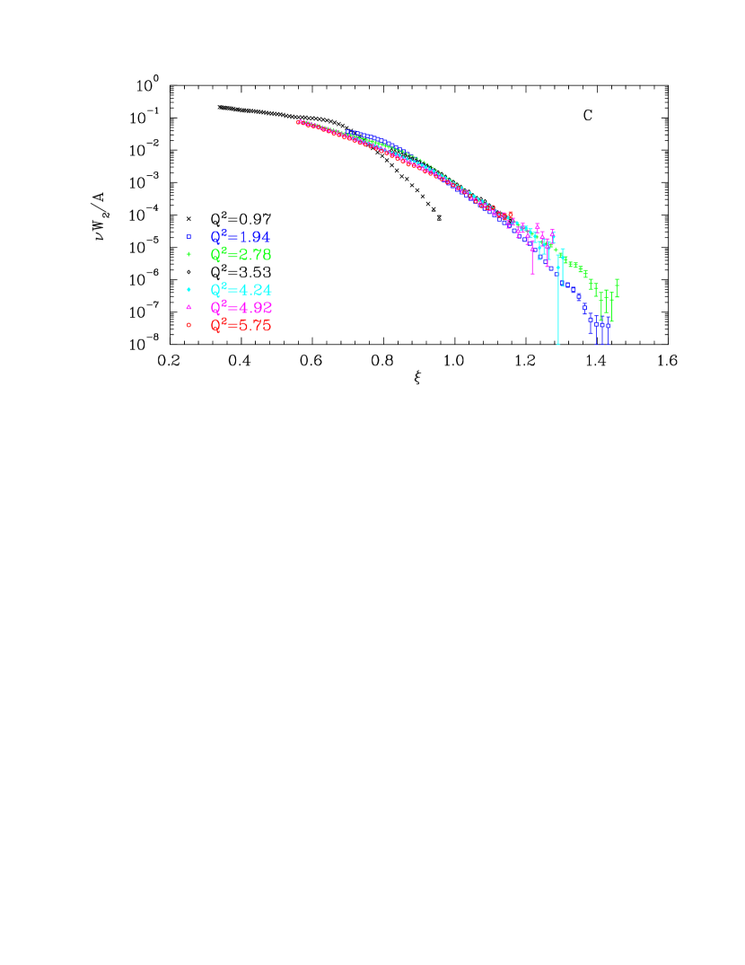
Figure 5.18: Carbon structure function, $\nu W_{2}^{C}(\xi,Q^{2})$. Errors shown are statistical only. The $Q^{2}$ values indicated are for $x=1$.

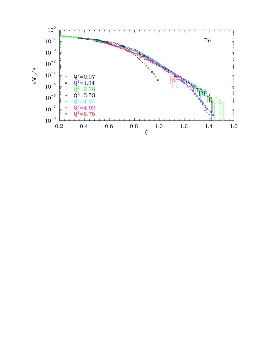
Figure 5.19: Iron structure function, $\nu W_{2}^{Fe}(\xi,Q^{2})$. Errors shown are statistical only. The $Q^{2}$ values indicated are for $x=1$.

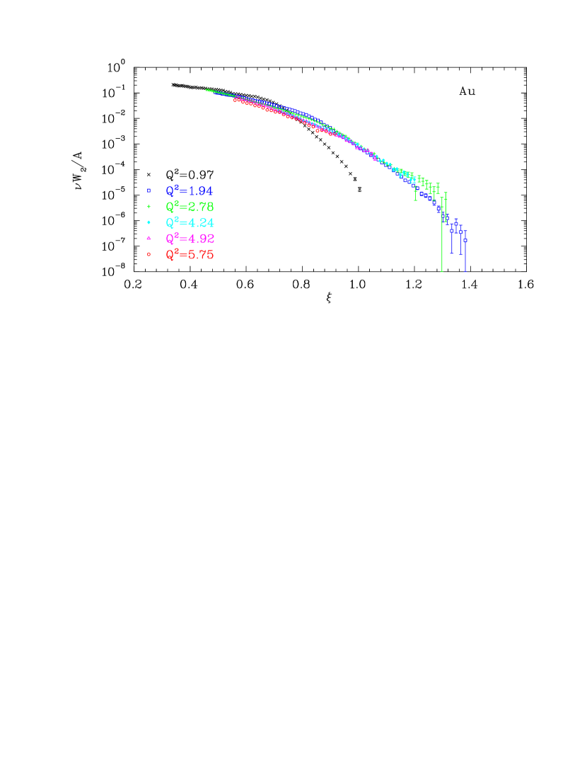
Figure 5.20: Gold structure function, $\nu W_{2}^{Au}(\xi,Q^{2})$. Errors shown are statistical only. The $Q^{2}$ values indicated are for $x=1$.

When examined at fixed $\xi$, the $Q^{2}$ behavior of the structure function is very different than when examined at fixed $x$. While the structure function showed signs of scaling vs. $x$ only for the lowest values of $x$, approximate scaling occurs for all $\xi$ at the larger values of $Q^{2}$. At the lowest $\xi$ values, below the quasielastic peak for all angles, the structure function shows scaling at low $Q^{2}$. For high values of $\xi$, the structure function approaches the high-$Q^{2}$ value from below. In the intermediate $\xi$ region ($\xi\sim 0.8-1.0$), the structure function increases as the quasielastic contribution reaches it’s maximum, and then falls to the high-$Q^{2}$ value. While the quasielastic peak is fixed at $x=1$, it occurs at $\xi=2/(1+\sqrt{1+4M^{2}/Q^{2}})$, increasing towards $\xi=1$ as $Q^{2}$ increases. Therefore, $\xi=0.8$ is above the quasielastic peak (corresponds to $x>1$) at low $Q^{2}$, is on top of the quasielastic peak at $Q^{2}\simeq 2.8$ (GeV/c)², and is below the peak at larger $Q^{2}$. Figure 5.21 shows the contribution to the structure function from quasielastic scattering and inelastic scattering for a fixed value of $\xi$. The quasielastic and inelastic contributions are taken from the model described in section 3.4. Figures 5.22 and 5.23 show the $Q^{2}$ dependence of the structure function for several values of $\xi$. The errors shown do not include the contribution coming from the uncertainty in $R=\sigma_{L}/\sigma_{T}$ because it is highly correlated for the different $Q^{2}$ values.

Figure 5.21: Structure function at fixed $\xi=0.85$ vs. $Q^{2}$. The dashed and dotted lines are the quasielastic and inelastic contributions from the model described in section 3.4. While the NE11 [94] and NE18 [25] measurements extend to higher $Q^{2}$ values than the present measurement, they are taken in the vicinity of $x\approx 1$. Therefore, the coverage in $\xi$ is limited to $0.6\mathrel{\raise 1.29167pt\hbox{$<$}\mkern-14.0mu\lower 2.58334pt\hbox{$\sim$}}\xi\mathrel{\raise 1.29167pt\hbox{$<$}\mkern-14.0mu\lower 2.58334pt\hbox{$\sim$}}1.0$, with low $Q^{2}$ values at low $\xi$, and higher $Q^{2}$ values at high $\xi$.

Figure 5.22: Structure function for Iron at fixed $\xi$ vs. $Q^{2}$. Solid symbols are e89-008 data, and hollow symbols are data from NE3. Statistical and total uncertainties are shown (excluding systematic uncertainty from the knowledge of $R=\sigma_{L}/\sigma_{T}$).

Figure 5.23: Structure function for Iron at fixed $\xi$ vs. $Q^{2}$. Solid symbols are e89-008 data, and hollow symbols are data from NE3. Statistical and total uncertainties are shown (excluding systematic uncertainty from the knowledge of $R=\sigma_{L}/\sigma_{T}$).

The scaling of $\nu W_{2}$ as a function of $\xi$ has been interpreted to be a consequence of the observed Bloom-Gilman duality in electron-nucleon scattering (see section 4.5) which suggests that when taken over a finite region in $\xi$, the $Q^{2}$ behavior of the quasielastic peak and resonances matches the behavior of the deep inelastic structure function. If the momentum distribution of the nucleons sufficiently averages the distribution, then the behavior of the structure function in the resonance region should match the behavior in the deep inelastic limit for all $\xi$ values, even if there are still large contributions to the cross section from quasielastic and resonance scattering.

An alternative explanation has been proposed by by Benhar and Luiti [37]. They explain the observed scaling at high $\xi$ values in terms of the $y$-scaling of the quasielastic cross section. They suggest that the $Q^{2}$ dependence that arises from examining $\xi$ rather than $y$ (as discussed in section 4.5) is cancelled by the $Q^{2}$ dependence of the final-state interactions. Expanding $y$ (for nuclear matter) in terms of $\xi$, gives:

$$y=y_{0}(\xi)-\frac{M_{N}^{3}\xi}{Q^{2}}+O(1/Q^{4}),$$ (5.10)

with $y_{0}(\xi)\equiv M_{N}(1-\xi)-E_{min}$. Therefore, $y$ is not just a function of $\xi$, it has an additional $Q^{2}$ dependence, and the data should not scale in $\xi$ until the $Q^{2}$ dependence becomes very small. However, final-state interactions introduce a modification to the cross section, which can be expressed in terms of a shift in $y$. They calculate the final-state interactions (using the approach of [109]) and write $F(y)$ in terms of the PWIA scaling function at a modified value of $y$:

$$F(y)=F_{IA}\left(y_{0}(\xi)-a_{\xi}(Q^{2})+b_{FSI}(y,Q^{2})\right)$$ (5.11)

where $a_{\xi}(Q^{2})$ is the $Q^{2}$ dependent term in the translation from $\xi$ into $y$ ($a_{\xi}(Q^{2})=\frac{M_{N}^{3}\xi}{Q^{2}}+O(1/Q^{4})$). They find that for $Q^{2}\mathrel{\raise 1.29167pt\hbox{$>$}\mkern-14.0mu\lower 2.58334pt\hbox{$\sim$}}3$ (GeV/c)², $a_{\xi}(Q^{2})$ and $b_{FSI}(y,Q^{2})$ largely cancel ($a_{\xi}(Q^{2})$ + $b_{FSI}(y,Q^{2})$ is roughly constant). Thus, the final state interactions cancel the variation in the scaling function coming from taking fixed $\xi$ rather than fixed $y$.

However, while there may be significant cancellation between the $Q^{2}$ dependence that comes from the transformation from $y$ to $\xi$ and the $Q^{2}$ dependence of the final-state interactions, the cancellation is not complete, and the data (which exhibit scaling in $F(y)$ as a function of $y$) do not show scaling when taken as a function of $\xi$. Figure 5.24 shows the quasielastic scaling function $F(y)$, taken as a function of $\xi$. The data do not appear to scale in the quasielastic scaling function when taken as a function of $\xi$. While the data may be closer to showing scaling than in the absence of the final-state interactions, the $Q^{2}$ dependence at high $\xi$ values is significantly larger than seen in the structure function $\nu W_{2}(\xi,Q^{2})$.

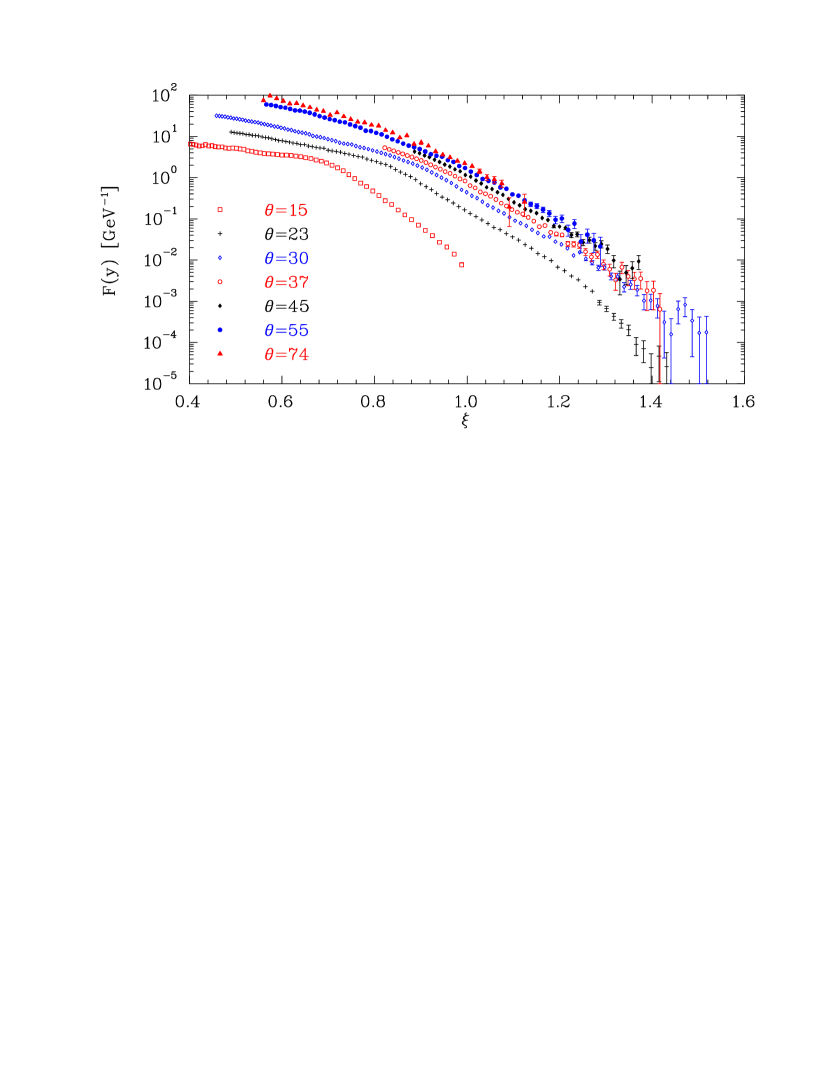
Figure 5.24: Scaling of the quasielastic scattering as a function of $\xi$. The plot shows the quasielastic scaling function $F(y)$, but as a function of $\xi$. The data are measurements on Iron with statistical uncertainties only.

In addition, while $F(y)$ appears to scale in $y$, the structure function $\nu W_{2}$ does not (see figure 5.25). Therefore, even if the cancellation between the $Q^{2}$ dependence of the transformation of variables and the final-state interactions is complete, the structure function would not show scaling in $\xi$. The $Q^{2}$ dependence would be as large as it is when taken as a function of $y$. Therefore, it appears that the observed $\xi$-scaling behavior of the structure function arises from something more than just the $y$ scaling of the quasielastic data and an accidental cancellation of $Q^{2}$ dependent effects.

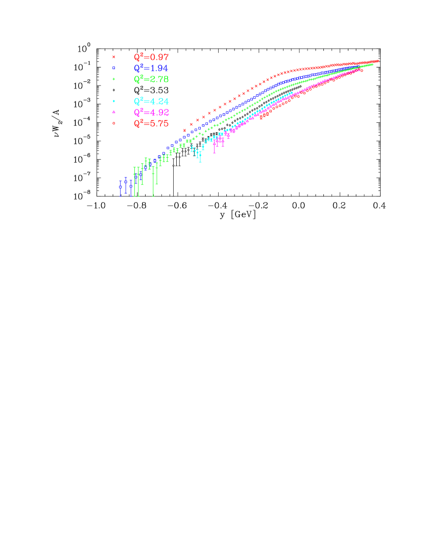
Figure 5.25: Iron structure function versus $y$. The plot shows the structure function $\nu W_{2}$ as a function of $y$. While $F(y)$ shows scaling in this $Q^{2}$ range, $\nu W_{2}$ does not. The data are measurements on Iron from NE3.

5.9 $A$-dependence

Figures 5.26 and 5.27 show the structure function per nucleon for Carbon, Iron, and Gold as a function of $x$ for $\theta$=23^∘ and 55^∘. The quasielastic peak is more pronounced in the lighter target, because the average nucleon momentum is larger for the heavier target, leading to a broadening of the quasielastic peak. This effect is smaller at the larger angles because the inelastic contribution becomes significant compared to the quasielastic for the larger angles. For $0.5<x<0.9$, we see a decrease in the structure function per nucleon as $A$ increases, corresponding to the the EMC effect [9] as observed in the EMC ‘large $x$’ data. For $x>1$, the structure function is larger for the heavier nuclei, due to the broadening of the nucleon momentum distribution. However, much of the strength at $x>1$ comes from nucleon-nucleon correlations in the nucleus [110] which are relatively $A$-independent for $A\mathrel{\raise 1.29167pt\hbox{$>$}\mkern-14.0mu\lower 2.58334pt\hbox{$\sim$}}12$. Therefore, the ratio of structure functions does not continue to rise as $x$ increases, as would be expected for, e.g., gaussian broadening of the quasielastic peak.

Figure 5.26: The top figure shows $\nu W_{2}/A$ for Carbon, Iron, and Gold at 23^∘. Near the quasielastic peak ($x\approx 1$), the structure function decreases as $A$ increases, due to the momentum distribution of the nucleus smearing out the peak. As $A$ increases, the peak becomes shorter and wider. For large $x$ values, the structure function increases somewhat with increasing $A$. The bottom figure shows the ratio of Gold to Iron and Iron to Carbon. Errors shown are statistical only. There is a systematic uncertainty of $\sim$5% in the ratio.

Figure 5.27: The top figure shows $\nu W_{2}/A$ for Carbon, Iron, and Gold at 55^∘. Near the quasielastic peak ($x\approx 1$), the structure function decreases as $A$ increases, but it is a smaller effect at 55^∘ because the cross section has a somewhat larger contribution from inelastic scattering than from quasielastic scattering. For large $x$ values, the structure function increases slightly with increasing $A$. The bottom figure shows the ratio of Gold to Iron and Iron to Carbon. Errors shown are statistical only. There is systematic uncertainty of 5-6% in the ratio.

Only statistical uncertainties are shown in the figures. The systematic uncertainties are $\sim$3.5-4.0% (3.5-4.5% at 55^∘) in each data set, and are mostly uncorrelated between the different targets due to the current radiative correction procedure (see section 3.3.10). The radiative correction procedure will be modified in order to study the $A$-dependence more carefully once the Deuterium data has been analyzed. This will not improve the systematic uncertainties in the measure cross section, but will cause the errors to be correlated between the different targets, thus decreasing the systematic uncertainty in the ratios. In addition, the deuterium data will allow us to directly generate EMC-like ratios for the data at $x>1$, and allow a more direct examination of short range correlations and deuteron-like configurations in the nucleus (see [110, 111, 13, 78]).

Chapter 6 Summary and Conclusion

Results have been shown for the cross section, $y$-scaling function, and structure function for inclusive electron scattering from Carbon, Iron, and Gold for values of $Q^{2}$ between 0.8 and 7.3 (GeV/c)². Where possible, the data start well below the elastic peak ($x\mathrel{\raise 1.29167pt\hbox{$>$}\mkern-14.0mu\lower 2.58334pt\hbox{$\sim$}}0.5$) and are cross-section limited at high $x$ values. Data were also taken on Deuterium, and these results will be published at a later date.

The $y$-scaling function, $F(y)$, has been extracted to extremely high $|y|$ ($y\approx-800MeV/c$ for $Q^{2}\mathrel{\raise 1.29167pt\hbox{$<$}\mkern-14.0mu\lower 2.58334pt\hbox{$\sim$}}3.0$, $y\approx-500MeV/c$ for $Q^{2}$ up to $\sim$5.0 GeV/c). At moderate values of momentum transfer, the scaling breaks down for $y\mathrel{\raise 1.29167pt\hbox{$>$}\mkern-14.0mu\lower 2.58334pt\hbox{$\sim$}}0$, and at the highest values of $Q^{2}$, scaling violations are seen as low as $y\approx-250MeV/c$. for $Q^{2}\mathrel{\raise 1.29167pt\hbox{$>$}\mkern-14.0mu\lower 2.58334pt\hbox{$\sim$}}3.0$, the scaling is very good and final-state interactions seem to be small GeV/c², but from the observations of scaling alone, it is not possible to determine if the final-state interactions are negligible, or if they are still significant, but have a small $Q^{2}$ dependence. These measurements of $F(y)$ can be used to examine the momentum distribution of nucleons in the nucleus, and complement exclusive measurements of the momentum distribution at CEBAF and elsewhere [112, 113] with significant coverage at large $|y|$.

The structure function is examined for scaling of the inelastic scattering, and scaling in $x$ is seen only at the lowest values of $x$ measured ($x\mathrel{\raise 1.29167pt\hbox{$<$}\mkern-14.0mu\lower 2.58334pt\hbox{$\sim$}}0.5$). This is not surprising, as the success of the $y$-scaling at $y\mathrel{\raise 1.29167pt\hbox{$<$}\mkern-14.0mu\lower 2.58334pt\hbox{$\sim$}}0$ ($x\mathrel{\raise 1.29167pt\hbox{$>$}\mkern-14.0mu\lower 2.58334pt\hbox{$\sim$}}1$) indicates the dominance of the quasielastic cross section. However, while we are not in the scaling regime for the inelastic contributions, the $A$-dependence of the structure function (as a function of $x$) can be used to examine the effects of the nuclear medium on the quark momentum distributions in the nucleus. For $x>1$, the $A$-dependence, and especially the ratio of the heavier nuclei to deuterium, is sensitive to the details of the high-momentum components of the momentum distribution.

When the structure function is examined as a function of $\xi$, the data do appear to scale. It has been suggested that this may be a consequence of Local Duality, where the structure of the quasielastic form factors is washed out by the nucleon motion, and the quasielastic and inelastic structure functions have the same $Q^{2}$ dependence. The data are consistent with scaling for low and high values of $\xi$ ($\xi\mathrel{\raise 1.29167pt\hbox{$<$}\mkern-14.0mu\lower 2.58334pt\hbox{$\sim$}}0.7$ and $\xi\mathrel{\raise 1.29167pt\hbox{$>$}\mkern-14.0mu\lower 2.58334pt\hbox{$\sim$}}1.0$), with small but non-negligible $Q^{2}$ dependence for intermediate values of $\xi$.

Additional information will become available when the analysis of the Deuterium data is complete. The deuterium data will allow us to compare target ratios for $x>1$, and allow us to compare the high-momentum components of the wavefunction for the different nuclei. In addition to including the deuterium in the analysis, the improvement in the radiative correction procedure (described in section 3.3.10) will reduce the systematic uncertainties in the $A$-dependence analysis of the data. Finally, an extension of the experiment up to 6 GeV beam energies has been approved at CEBAF [114]. The increase from 4 GeV to 6 GeV will give a small increase in the $Q^{2}$ coverage for $x\mathrel{\raise 1.29167pt\hbox{$>$}\mkern-14.0mu\lower 2.58334pt\hbox{$\sim$}}2$, but a significant increase ($\sim$50%) in the $Q^{2}$ range for intermediate $x$ and $y$ values ($1\mathrel{\raise 1.29167pt\hbox{$<$}\mkern-14.0mu\lower 2.58334pt\hbox{$\sim$}}x\mathrel{\raise 1.29167pt\hbox{$<$}\mkern-14.0mu\lower 2.58334pt\hbox{$\sim$}}1.8$, $|y|\mathrel{\raise 1.29167pt\hbox{$<$}\mkern-14.0mu\lower 2.58334pt\hbox{$\sim$}}500MeV/c$). Because the high-$x$ data comes from relatively low $Q^{2}$ measurement, the large $x$ region between ($2<x<4$) maps into a small range in $\xi$ ($1.4\mathrel{\raise 1.29167pt\hbox{$<$}\mkern-14.0mu\lower 2.58334pt\hbox{$\sim$}}\xi\mathrel{\raise 1.29167pt\hbox{$<$}\mkern-14.0mu\lower 2.58334pt\hbox{$\sim$}}1.7$). Therefore, the $Q^{2}$ coverage will increase significantly for most of the $\xi$ range.

This thesis and tables of cross sections, $F(y)$, and $\nu W_{2}$ values will be available over the web at http://www.krl.caltech.edu/$\sim$johna.

Appendix A Hall C Analysis Engine

A.1 Engine Overview

The event decoding and reconstruction and the analysis of scalers and slow controls was done using the standard Hall C analysis software (the Hall C Engine). The Engine uses a minimal set of the CEBAF Online Data Acquisition (CODA) routines in order to unpack the raw CODA physics, scalar, and control events. In addition to the event reconstruction and data analysis in the Engine, there is a test/histogramming package (‘CTP’ - the CEBAF Test Package) and an event display/debugger (‘evdisplay’).

A.2 CEBAF Test Package

The CEBAF Test Package (CTP) [62] software was written in C by Stephen Wood at CEBAF to provide a flexible way to define and evaluate tests, histograms, and scalers. It also allows the storage, modification, and sharing of other analysis parameters. CTP is modeled loosely on the LAMPF Q system [63]. In order for CTP to share variables with the Fortran code, the variables must be registered using calls to CTP subroutines. In the Hall C engine, all common blocks are contained in .cmn files. When the code is compiled, these files are parsed and all of the variables defined in the common blocks are automatically registered. They are then accessible from both the Fortran source code and from CTP. The variables can then be examined or changed without recompiling code. CTP uses remote procedure calls (RPC) to access these shared variables. In addition, variables that are not part of the engine’s Fortran code can be defined in CTP input files and used to create tests and to define histograms.

The analysis engine primarily uses CTP to input parameters and run time flags that control the analysis, and to define the histograms, tests, and scalar reports to be output. The input parameters and the histogram and test definitions are stored in ASCII files and read in at the beginning of the analysis code. At the end of each event, the CTP tests are evaluated. Then, histograms are filled and software scalars incremented using the results of the tests.

CTP’s ability to examine and modify variables in the Engine is used by the event display code (evdisplay) in order to give a graphical representation of an event. In addition to displaying hits in the detectors and tracking information, the event display also acts as a user interface to the analysis code. By defining CTP tests in the event display, one can set conditions for the events to be displayed. This allows selection of events to examine based on raw hits, decoded detector information, and tracking and particle identification information. Once an event is selected, any registered variable can be examine or modified. This event selection and examination capability makes the event display a useful tool for debugging both hardware and analysis problems.

A.3 Analysis Engine

The flow of the analysis code is shown in figure A.1. The subsections of the code are described below.

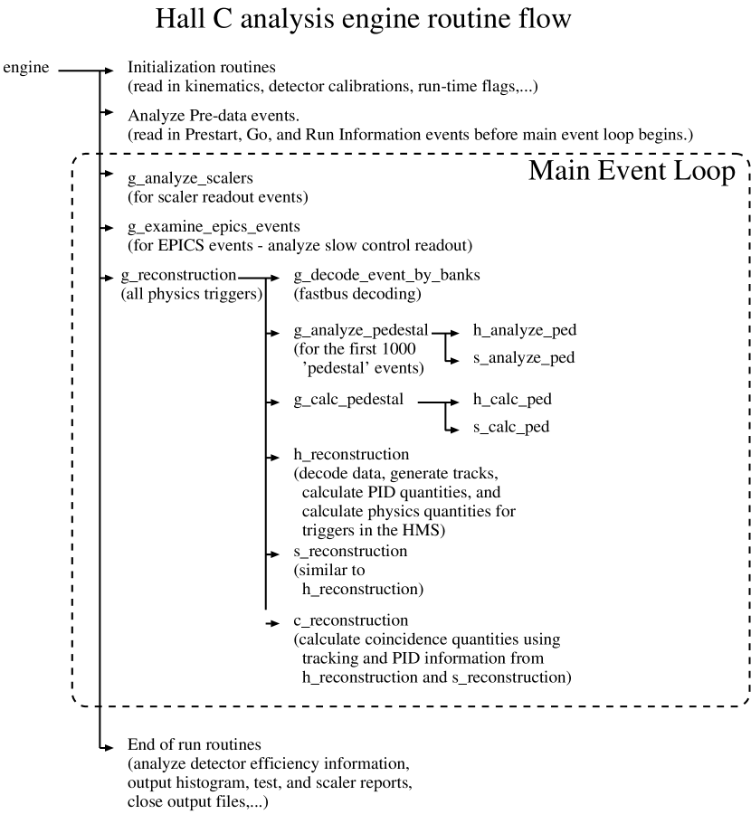
Figure A.1: Software flow diagram for the Hall C analysis engine.

A.3.1 Initialization

The engine starts by reading in the main configuration file, defined by an environment variable. This file contains several runtime flags and pointers to the data file, the output files, and several parameter files. Some of the files set the parameters that define the locations, calibrations, and decoding of the detector elements. Others are used to define CTP histograms, tests, and scalers. Output filenames are given, as well as template files which define the histograms and scalers to be output. Kinematics and other quantities that vary run to run are read from a separate parameter file. After all of the run parameters are defined, the PAW (Physics Analysis Workstation) HBOOK and Ntuple initializations are performed, and the raw data input file is open. CTP statements can be entered at the command line and override values taken from any of the input files or the default values. This can be used to set run time flags, or override any of the parameters read from the kinematics or database files. After initializations are completed, the engine then begins looping through the events in order to analyze the beginning of run information events. These include CODA status events, readback values of the ADC (Analog-to-Digital Converter) thresholds, runtime options, and kinematics input by hand at the beginning of each run. Once these initialization events have been analyzed, the main event loop begins.

A.3.2 Main Event Loop

In the main event loop, each event is read in and then processed according to the event type. If the event is a scalar read, it is analyzed and the total counts and change in counts are recorded for each of the hardware scalers. In addition, the time and accumulated charge since the last event are calculated, and the total charge is incremented.

If the event is an EPICS (Experimental & Physics Industrial Control System) read event, the EPICS variables are stored. The HMS (High Momentum Spectrometer) magnet settings are compared to the expected value for the desired momentum of the run (the SOS (Short Orbit Spectrometer) magnet settings were not accessible to the EPICS database during e89-008), and the target position readback values are compared to the expected values for the desired target. Quantities related to the beam position monitors in the Hall C Arc and beamline, and the beam energy as determined by the Arc are written to an EPICS summary file, along with diagnostics information from the cryotarget.

Finally, if the event is a physics event, it is analyzed. There are four types of physics triggers. At the beginning of each run, 1000 pedestal (PED) triggers are taken. These are triggers generated by a pulser, and contain data from all of the ADCs. These values are used to determine the pedestal value for each ADC channel. The calculated pedestals are subtracted from the ADC values for each event. In addition, a threshold is calculated for each ADC input (15 channels above pedestal). The thresholds are compared to the values that were programmed into the ADC for that run, and warning messages are generated for signal with improper thresholds in the ADC. For each run, a file of thresholds is generated, and can be used to update the thresholds that are programmed into the ADCs at the beginning of each run.

The other physics event types are HMS, SOS, and COIN. These are the events caused by the real spectrometer triggers. The raw detector hits are read in for these events and passed to the main reconstruction routine for the HMS and/or SOS. The event is reconstructed, and tracking and particle identification information stored for each spectrometer. Cuts on the tracks are applied and then physics quantities are calculated for singles triggers in each spectrometer, and for coincidence events if both spectrometers fired. After each event is tracked, CTP tests are evaluated and scalars and histograms incremented. In addition, there are routines that keep statistics on tracks and detector hits in order to measure the efficiency of each detector element. These are calculated at the end of the analysis, and detectors with low efficiencies are noted.

A.3.3 Event Reconstruction

Figure A.2: Software flow diagram for the HMS event reconstruction code.

The general flow of the event reconstruction routine is as follows. First, tracking independent quantities are calculated for the hodoscopes, calorimeter, and drift chamber hits. Next, the tracking routine is called, and a list of possible tracks is generated. For each of these tracks, track dependent quantities are recorded for the hodoscopes and calorimeter. User defined cuts are then applied in order to reject ‘bad’ tracks, and of the ‘good’ tracks, the one with the best $\chi^{2}$ is chosen as the final track. For the final track, physics quantities are calculated and recorded. Finally, scalers used to measure the detector efficiencies are incremented.

The reconstruction code is nearly identical for the two spectrometers, except for the aerogel analysis in the SOS and geometry differences between the HMS and SOS drift chambers. The data structures and analysis code are the same for the HMS and SOS detectors, and for the most part only the names and parameters are different for the two spectrometers. Figure A.2 shows the flow diagram for the HMS reconstruction. The SOS is identical except for the addition of code that analyzes the aerogel Čerenkov.

First, the hodoscope hits are translated from raw ADC and TDC (Time-to-Digital Converter) values to pulse heights and times. Timing corrections due to pulse height variations, cable length offsets, and signal propagation through the scintillator element are applied. Events outside of a user defined timing window are discarded to eliminate random hits. The time measured in each scintillator plane is used to determine the time that the particle passed through the scintillators. This time is used as as the start time for the drift chambers. The difference between the start time and the drift chamber TDC measurement is the time it took for the signal from the particle passing through the drift chamber gas to reach the wire. This drift time will be converted into a drift distance in order to determine the distance between the point where the particle passed and the center of the wire.

After the hodoscopes have been decoded and the start time determined, the drift chamber, calorimeter, and Čerenkov hits are decoded and track independent quantities are calculated. For the drift chamber, a list of hit wires is generated, containing the plane and wire number of the hit wire, and the TDC value. For the Čerenkov, the ADC value for each tube is recorded, as well as the number of photoelectrons in each tube and the total sum. The calorimeter generates a list of blocks which measure energy deposition above a software threshold. For each hit, the raw ADC value and the energy deposited are kept. In addition, the total energy in each layer as well as the energy in the entire calorimeter are calculated. Finally, the ADCs containing event by event beamline information are decoded.

Next, the tracking routine is called. The details of the tracking algorithm are described in the Event Reconstruction chapter. For each chamber, clusters of hits (space points) are identified, and mini-tracks (stubs) are fitted to the single chamber space points. The tracking routine loops over all combination of stubs in the two chambers, and fits a full track if the two stubs are consistent. The focal plane track is reconstructed to generate a track at the target. All tracks found are kept, and tracking dependent quantities are calculated for each track.

For each track, the time of flight is calculated. The focal plane track is used to identify hodoscope elements corresponding to that track. The track must point within 2 cm of the track to be included in the time of flight calculation. The time from each photomultiplier tube (PMT) is corrected for propagation time along the scintillator (using the track to determine the distance from the PMT), the pulse height walk, and offset for that particular PMT. If both PMTs on a scintillator have a time, they are combined to form a mean time for that element. Both PMTs are required to have a good time in order to be used in the time of flight fit. As long as this does not cause a significant inefficiency, it reduced the uncertainty in the time measurement, as the velocity corrections will cancel. If the track points to adjacent elements that both have hits, then the two scintillator mean times will be averaged in order to generate the time for that hodoscope plane. If at least one of the front plane (S1X or S1Y) and one of the back (S2X or S2Y) have a good time, a least-squares fit of the time of flight is made based on the times, $z$-positions of the hodoscope elements (taking into account the staggering of the adjacent elements), and the angle of the track. Using this velocity and the momentum of the particle (as determined by the track reconstruction), the mass of the particle can be determined from:

$$\beta=\frac{p}{E}=\frac{p}{\sqrt{p^{2}+m^{2}}}.$$ (A.1)

In addition to calculating the particle velocity and mass, the energy deposition ($dE/dx$) is calculated for each plane. In order to negate the effect of attenuation, both PMTs are required to have an ADC value, and the $dE/dx$ for the plane is taken as the geometric mean of the two ADC values. For exponential attenuation, this quantity will be independent of hit position. $dE/dx$ can be used to help separate slower hadrons, but was not used as a particle identification test for e89-008.

Quantities used for particle identification are then calculated for each track that was found. First, clusters of hits are found in the lead glass blocks, and the energy per layer and total energy associated with each cluster are calculated. For each track, the calorimeter energy associated with the track is the energy in the cluster the track points to, if any. The track must point to within 3cm of the center of the cluster in order to be associated with the shower. The energy is then corrected for attenuation in the lead glass modules, using the track to determine the distance from the PMT of the hit. For the Čerenkov, all tracks use the sum of all four mirrors as the signal.

After the timing and particle identification (PID) quantities have been calculated for each track, hard cuts are applied to reject bad tracks. Cuts are applied on the $\chi^{2}$ of the track, $dE/dx$ in the hodoscopes, the particle velocity, and the calorimeter total energy, and events that fail these cuts are rejected. These cuts serve two purposes. The particle identification cuts can be used to reject tracks corresponding to particles that are a background for the measurement. In addition, a cut on $\beta$ or $dE/dx$ can be used to insure that the track points to multiple scintillator elements, even if the cut is too loose to be used for particle identification. For e89-008, these cuts were opened up and all tracks were kept. Because the rate of true multiple tracks is very small (almost always $<$0.1%), we assumed that there was only one particle in the spectrometer, and did not use these cuts to differentiate between pions and electrons in a single trigger. If multiple tracks pass these cuts, then the track with the best $\chi^{2}$ is selected as the final track. There are typically multiple tracks in 1-2% of the events, and these usually come from events where two nearly identical space points are found in a single chamber, where 5 of the wires are included in both space points, and the sixth wire differs (or is missing). This usually gives two very similar tracks, and selecting the best $\chi^{2}$ is effective in selecting the appropriate track.

For the final track, the desired physics quantities are calculated, and the CTP tests are evaluated and scalers and histograms incremented for the singles events. If there was a final track in both spectrometers, the coincidence physics quantities are calculated, and coincidence tests, scalers, and histograms are evaluated and incremented.

After all information for the event has been saved, the tracking information is used to measure the efficiency of each detector element. The general procedure is to use the track to determine which detector elements should have had a signal. A counter of the number of expected hits is incremented for each element which should have had a signal, and if that element did have a signal, a counter of actual hits is incremented as well. Because of uncertainty in the reconstruction and multiple scattering of the electron, we require that a track point near the center of the detector element before declaring that the detector should have had a hit. For the drift chambers, the track must pass within 0.3 cm of the wire. For the hodoscopes, the track must be at least 2 cm inside of the edge of the HMS elements, and 1 cm inside the edge of the SOS elements. Efficiencies for the PMTs on each end of the element, as well as the efficiency of both firing together are calculated. Because of the multiple scattering in the detector, runs at lower momenta ($\mathrel{\raise 1.29167pt\hbox{$<$}\mkern-14.0mu\lower 2.58334pt\hbox{$\sim$}}$1.5 GeV/c) showed a lower hodoscope efficiency for the rear planes. This was because the multiple scattering in the front hodoscopes could deflect the particle enough that it sometimes missed the rear elements, even though the track at the drift chambers pointed at the center of an S2X or S2Y element. This problem was worse in the SOS, because the Y elements were only 4.5 cm wide. Therefore, even if only tracks pointing to the central 0.5cm of the element were examined, 2 cm of multiple scattering would cause an inefficiency to appear in the calculation, even though the element may have been 100% efficiency. Therefore, the hodoscope efficiencies were used to monitor the SOS hodoscope trigger efficiency, but not to calculate a correction for the inefficiency. For the calorimeters, the track must point within 2 cm of the edge, and have a Čerenkov signal to insure that the particle is an electron and will leave a large signal in the calorimeter. In the Čerenkov, the track is used to determine what mirror the track points to. The event is required to have a good time of flight and calorimeter signal for an electron ($\beta\approx 1$, $E>1$GeV). The efficiency is calculated for each mirror, and for the entire Čerenkov area.

In order to insure that the track is reconstructed well in the drift chamber, a cut is applied to the $\chi^{2}$ of the track fit before a track is used to measure the efficiency. All tracks with a low $\chi^{2}$ are used in the efficiency calculation, except for the Čerenkov and calorimeter which have PID cuts. This means that if the efficiency is different for different particle types, then the measured efficiency may not reflect the efficiency for the events of interest. However, for e89-008 the efficiencies were close enough for electrons and pions that the calculated values were sufficient for monitoring the drift chamber and hodoscope efficiencies.

Finally, after the HMS and/or SOS tracks have been reconstructed, a call is made to the CTP routines which evaluate the user defined tests and increment the scalers and histograms.

A.3.4 Efficiency Calculations

After the last trigger is analyzed, the efficiency scalers for each detector element are used to determine the efficiency for each element. If the efficiency is below a threshold given for the detector, that element is included in a list of possible bad elements. Finally, the efficiencies of the individual elements are used to calculate overall plane and detector efficiencies. These are used to calculated the expected trigger efficiency for the hodoscopes (which require hits with both PMTS in three of the four planes to fire), and the tracking efficiency for the drift chambers (which requires five of six planes to fire in each chamber).

A.3.5 Output

When the end of the run event is encountered, the engine writes the output files. Scalar report files contain the final values for the hardware and software scalers, as well as the accumulated charge, measured detector efficiencies, and dead time correction factors. The histogram files primarily contain detector summary histograms, so that the detector performance can be monitored online and the calibrations can be checked offline. The Ntuple files contain the event by event information. Tracking information, reconstructed quantities, and particle ID information are contained in the Ntuple, and cuts on the reconstructed or PID quantities can be applied.

Appendix B Trigger Supervisor

The interface between the trigger hardware and the computer data acquisition system is the trigger supervisor (TS). The TS makes all of the ‘decisions’ about how to process the triggers it receives, choosing which triggers to respond to as well as determining the current state of the run. The TS splits the run into two parts, allowing us to sparsify the ADCs and still record the pedestal values for each channel. In order to reduce the event size, we used the sparsification feature of our ADCs and TDCs. The TDCs normally operate in sparsified mode, giving an event for a channel only if it received a stop signal after the common start. The LeCroy 1881M ADCs can be programmed to ignore all channels that have a signal smaller than a threshold value which can be set for each channel. However, using the sparsification means that we do not get pedestal values for each channel during normal data taking. To determine the pedestal values, we divide up the run into two different phases. First, we take a fixed number of events (usually 1000) generated by a random trigger while data sparsification is disabled and the real triggers are blocked. This allows us to measure the pedestal values for the ADCs. After these events, we enable sparsification and block the random triggers, taking only the real triggers. The data acquisition mode is controlled using the TS status outputs. There are three outputs from the TS that determine how events will be processed. The TS GO signal is active at all times when a run is in progress. The TS enable1 (EN1) signal indicates that a run is in progress and normal data taking in enabled. Finally, the TS BUSY signal is active whenever the TS is busy processing an event. During a normal run, the following sequence of events occurs: first, the TS GO signal comes on, and we generate pedestal triggers (from a pulser). After 1000 events the ADCs change over to sparsified mode and the TS sets the TS EN1 signal, enabling the physics triggers and blocking the pedestal triggers. In addition, the TS provides a busy signal that blocks triggers whenever the TS is busy processing an event.

The Trigger Supervisor provides all of the control signals, but in order to have an ‘external’ record of the logic that went into processing the event, the blocking of triggers due to the status of the TS is done in external logic and the intermediate steps are sent to scalers and TDCs to be recorded. The trigger signals (HMS, SOS, and PED triggers) and the TS control signals (GO, EN1, and BUSY) are fed into a LeCroy 8LM programmable logic module (2365). The 8LM has eight outputs. Four are used for the HMS, SOS, COIN, and PED pretriggers. A pretrigger is generated for each incoming pretrigger during the appropriate part of the run, even if the TS was busy (i.e. PED pretriggers are passed during the beginning of the run, and the HMS and SOS pretriggers are passed and coincidence pretriggers generated during the normal running). The other four outputs are the HMS, SOS, COIN, and PED triggers. These are identical to the pretriggers except that they also require that the BUSY signal is not on. These triggers are fed directly to the TS, and each one should cause an event to be read out. A prescaling factor can be set for each of the trigger types. TableB.1 shows the programming of the 8LM.

output signal		definition
HMS PRETRG	=	$(HMS)\&(EN1)$
SOS PRETRG	=	$(SOS)\&(EN1)$
COIN PRETRG	=	$(COIN)\&(EN1)$
PED PRETRG	=	$(PED)\&(GO)\&(\overline{EN1})$
HMS TRIG	=	$(HMS)\&(EN1)\&(\overline{BUSY})$
SOS TRIG	=	$(SOS)\&(EN1)\&(\overline{BUSY})$
COIN TRIG	=	$(COIN)\&(EN1)\&(\overline{BUSY})$
PED TRIG	=	$(PED)\&(GO)\&(\overline{EN1})\&(\overline{BUSY})$

Table B.1: 8LM trigger logic. The triggers are identical to the pretriggers except that the triggers require that the $BUSY$ signal is not active. The $EN1$ signal is used to block physics triggers during the pedestal running, and block pedestal triggers during normal data taking.

In addition to determining what types of triggers are to be processed, the trigger supervisor determines what hardware will be read out based on the trigger type. When a trigger arrives, the TS waits 7 ns and then latches all of the enabled trigger signals into a data word. It then uses a lookup table to determine what event type the trigger corresponds to and what gates need to be generated for data readout. Trigger signals which are prescaled away do not generate events, and are ignored when the TS latches the enabled trigger signals. There are four defined event types: HMS, SOS, COIN, and PED events. These do not exactly correspond to the incoming trigger types, because if multiple triggers come in, the TS has to decide what kind of event it is. For example, if both the HMS and SOS triggers come (or the COIN with anything else), the TS treats the event as a coincidence. Normally, there should be no ambiguity. PED triggers cannot come at the same time as any of the physics triggers, and the coincidence window in the 8LM is larger than the 7 ns the TS waits for triggers, so any HMS and SOS overlap in the TS should also form a COIN trigger in the 8LM. The singles triggers are delayed so that the COIN trigger will always reach the TS first. For PED and COIN triggers, gates go out to all of the fastbus modules (HMS, SOS, and beamline information), while for the singles triggers, only the appropriate spectrometer and beamline Fastbus modules receive gates and starts. For e89-008, the spectrometers were operated independently, and the only COIN triggers came from random coincidences between electrons in the two spectrometers and were prescaled away. However, even though the COIN triggers were prescaled away, if the HMS and SOS singles triggers came within the 7 ns TS trigger latching time, the event is treated as a coincidence.

After the HMS and/or SOS gates are generated by the TS, they are retimed with respect to the single arm trigger for that spectrometer. This is necessary for coincidences because the ADC gates must come at a fixed time with respect to the time the particle passed through the detector. The trigger for that spectrometer comes at a nearly fixed time with respect to the detected particle, but a coincidence trigger has its timing set by the later of the two spectrometers. Therefore, if the HMS came first, the timing of its ADC gates would be set by the SOS trigger for coincidence events, and the ADC gate might fail to properly overlap the signal it is supposed to integrate. The gates from the TS are then delayed and have their widths set so that they are timed properly for use as ADC gates and TDC starts. Figure B.1 shows the trigger supervisor related electronics.

Figure B.1: Trigger supervisor electronics.

References

- [1] R. K. Ellis, W. Furmanski, and R. Petronzio, Nucl. Phys. B212, 29 (1983).
- [2] S. A. Gurvitz, Phys. Rev. D 52, 1433 (1995).
- [3] B. L. Ioffe, V. Khoze, and L. N. Lipatov, Hard Processes (Horth-Holland, Amsterdam, 1984).
- [4] E. Pace, G. Salmè, and G.B.West, Phys. Lett. B 273, 205 (1991).
- [5] O. Greenberg, Phys. Rev. D 47, 331 (1993).
- [6] B.L.Ioffe, ZhEFT Lett. 58, 930 (1993).
- [7] E.Pace, G.Salmè, and A.S.Rinat, Nucl. Phys. A572, 1 (1993).
- [8] E. Pace, G. Salmè, and F. M. Lev, preprint hep-ph/9802020, 1998.
- [9] J. Aubert et al., Phys. Lett. B 123, 275 (1983).
- [10] J.D.Bjorken, Phys. Rev. 179, 1547 (1969).
- [11] G. B. West, Phys. Rep. 18, 263 (1975).
- [12] E. Pace and G. Salmè, Phys. Lett. B 110, 411 (1982).
- [13] D.B.Day et al., Annu. Rev. Nucl. Part. Sci. 40, 357 (1990).
- [14] J.D.Bjorken and E.A.Paschos, Phys. Rev. 185, 1975 (1969).
- [15] S. A. Gurvitz, A. Mair, and M. Traini, Phys. Lett. B 383, 233 (1996).
- [16] R. M. Barnett et al., Phys. Rev. D 54, 1 (1996).
- [17] H. Georgi and H. D. Politzer, Phys. Rev. D 14, 1829 (1976).
- [18] S. D. Drell and T. M. Yan, Phys. Rev. Lett. 24, 181 (1970).
- [19] G. B. West, Phys. Rev. Lett. 24, 1206 (1970).
- [20] E. Bloom and F. Gilman, Phys. Rev. D 4, 2901 (1971).
- [21] S.Rock et al., Phys. Rev. D 46, 24 (1992).
- [22] L.W.Whitlow et al., Phys. Lett. B 282, 475 (1992).
- [23] H. G. A. DeRujula and H. D. Politzer, Ann. Phys. 103, 315 (1977).
- [24] D. B. Day et al., Phys. Rev. Lett. 59, 427 (1987).
- [25] J. Arrington et al., Phys. Rev. C 53, 2248 (1996).
- [26] W. Schütz et al., Phys. Rev. Lett. 38, 259 (1977).
- [27] S.Rock et al., Phys. Rev. Lett. 49, 1139 (1982).
- [28] R. Arnold et al., Phys. Rev. Lett. 61, 806 (1988).
- [29] D. B. Day et al., Phys. Rev. Lett. 43, 1143 (1979).
- [30] J. S. McCarthy et al., Phys. Rev. C 13, 712 (1976).
- [31] B. Collaboration, Z. Phys C 63, 29 (1994).
- [32] C. Collaboration, Z. Phys C 49, 187 (1991).
- [33] M. Vakili, Ph.D. thesis, University of Cincinnati, expected 1998.
- [34] D. H. Potterveld, Ph.D. thesis, California Institute of Technology, 1989.
- [35] B. W. Filippone et al., Phys. Rev. C 45, 1582 (1992).
- [36] P. Bosted et al., Phys. Rev. C 46, 2505 (1992).
- [37] O. Benhar and S. Luiti, Phys. Lett. B 358, 173 (1995).
- [38] C. Yan et al., Nucl. Instrum. Meth. A365, 261 (1995).
- [39] P. Gueye, Status of the Actual Beam Position Monitors in the Hall C Beamline, CEBAF Internal Report (unpublished).
- [40] C. Yan, User’s manual of Hall C Beamline, CEBAF Internal Report (unpublished).
- [41] P. Gueye, M. Tiefenback, and C. Yan, Hall C Beam Energy Measurment, CEBAF Internal Report (unpublished).
- [42] D. Dutta et al., Beam Energy Determination Using Kinematic Methods, CEBAF Internal Report (unpublished).
- [43] E. Offermann et al., Phys. Rev. C 44, 1096 (1991).
- [44] G. Niculescu, Resonant Cavities used as Beam Current Monitors, CEBAF Internal Report (unpublished).
- [45] C. Armstrong, Beam Current Measurement in Hall C, CEBAF Internal Report (unpublished).
- [46] K. B. Unser, The Parametric Current Transformer, a Beam Current Monitor Developed for LEP, CERN SL/91-42 (unpublished).
- [47] F. Duncan, Hall C Cryogenic Target User Manual, CEBAF Internal Report (unpublished).
- [48] K. Gustafsson, Cryotarget Density Dependence on Beam Current, CEBAF Internal Report (unpublished).
- [49] R. Ent, private Communication.
- [50] J. Cobb and J. Murray, Nucl. Instrum. Meth. 46, 99 (1967).
- [51] CEBAF Conceptual Design Report (CEBAF press, Newport News, 1995).
- [52] M. Berz, COSY Infinity Version 7 Reference Manual, NSCL Technical Report MSUCL-977, Michigan State University, 1995.
- [53] D. C. Carey, K. L. Brown, and F. Rothacker, TRANSPORT, A Computer Program for Designing Charged Particle Beam Transport Systems, SLAC-R-95-462, 1995.
- [54] Experimental & Physics Industrial Control System (EPICS), Los Alamos National Laboratory, 1984.
- [55] O.K.Baker and other, Nucl. Instrum. Meth. A367, 92 (1995).
- [56] W. Smythe, CEBAF Hall C SOS Gas Cerenkov Detector Handbook, University of Colorodo, Boulder, Colorodo (unpublished).
- [57] H. Mkrtchyan (unpublished).
- [58] G. Heyes et al., in Proc. of the TOOLS 8 Conference (Prentice Hall, Santa Barbara, CA, July 1992), pp. 171–183.
- [59] G. Heyes et al., in Proc. of the CHEP Conference, edited by S. Loken (., San Francisco, CA, Apr. 1994), pp. 122–126.
- [60] D. Abbott et al., in Proc. of the IEEE Conference on Real-Time Computer Applications in Nuclear, Particle, and Plasma Physics, edited by R. Fox (Michigan State University - NSCL, East Lansing, 1995), p. 147.
- [61] C. Group, PAW (Physics Analysis Workstation) Users Guide, Program Library Q121, CERN.
- [62] S. A. Wood and W. A. W. III, in Conference Record of the Eigth Conference on Real-Time Computer Applications in Nuclear, Particla and Plasma Physica, edited by D. Axen and R. Poutissou (TRIUMF, Vancouver B.C. Canada, 1993), p. 60.
- [63] Introduction to Q, LAMPF internal report LA-7001-M, 1978.
- [64] J. L. Chuma, Physica analysis package, TRIUMF.
- [65] K. A. Assamagan, D. Dutta, and P. Welch, Hall C Matrix Element Optimization Package, CEBAF Internal Report (unpublished).
- [66] Stein et al., Phys. Rev. D 12, 1884 (1975).
- [67] L. W. Mo and Y. S. Tsai, Rev. Mod. Phys. 41, 205 (1969).
- [68] Y. S. Tsai, SLAC-PUB-848, SLAC Report (unpublished).
- [69] O. Benhar et al., preprint hep-ph/9706353, 1997.
- [70] M. F. Hutchinson, ACM Trans. Math. Softw. 12, 150 (1986).
- [71] H. Überall, Electron Scattering from Comples Nucli (Academic Press, New York, 1971), p. 210.
- [72] D. B. Day et al., Phys. Rev. C 40, 1011 (1989).
- [73] A. Bodek et al., Phys. Rev. D 20, 1471 (1979).
- [74] R. G. Arnold et al., Phys. Rev. Lett. 52, 727 (1984).
- [75] SLAC-PUB-3257, 1983.
- [76] S. Simula, private Communication.
- [77] C. C. degli Atti and S. Simula, Phys. Lett. B 325, 276 (1994).
- [78] C. C. degli Atti and G. B. West, preprint nucl-th/9702009, 1997.
- [79] T. G. O’Neill, Ph.D. thesis, California Institute of Technology, 1994.
- [80] N. C. R. Makins, Ph.D. thesis, Massachusettes Institute of Technology, 1994.
- [81] M. Gari and W. Krümpelmann, Phys. Lett. B 141, 295 (1984).
- [82] Walker et al., Phys. Rev. D 49, 5681 (1994).
- [83] A. E. L. Dieperink et al., Phys. Lett. B 63, 261 (1976).
- [84] T. D. Forest, Nucl. Phys. A392, 232 (1983).
- [85] R. D. McKeown et al., Phys. Rev. Lett. 56, 1452 (1986).
- [86] R. L. Jaffe et al., Phys. Lett. B 134, 449 (1984).
- [87] L. S. Celenza et al., Phys. Rev. C 31, 212; 232; 946 (1985).
- [88] G. B. West, preprint hep-ph/9612403, 1996.
- [89] G. Ricco et al., Phys. Rev. C 57, 356 (1998).
- [90] C. Keppel et al., in Proc. of the 6th Conference on Intersections Between Particle and Nuclear Physics, edited by T. W. Donnelly (AIP, Big Sky, MT, 1997), p. 585.
- [91] C. E. Keppel et al., CEBAF Approved Experiment E97-010, 1997.
- [92] O. Rondon et al., CEBAF Approved Experiment E96-002, 1996.
- [93] S.A.Gurvitz and A.S.Rinat, Phys. Rev. C 47, 2901 (1993).
- [94] P. Bosted et al., Phys. Rev. Lett. 49, 1380 (1982).
- [95] I. Sick, D. Day, and J. S. McCarthy, Phys. Rev. Lett. 45, 871 (1980).
- [96] P. D. Zimmerman, C. Williamson, and Y. Kawazoe, Phys. Rev. C 19, 279 (1979).
- [97] A.S.Rinat and M.F.Taragin, Nucl. Phys. A624, 773 (1997).
- [98] A.S.Rinat and M.F.Taragin, Nucl. Phys. A620, 417 (1997).
- [99] A.S.Rinat and M.F.Taragin, Nucl. Phys. A598, 349 (1996).
- [100] S. Simula, Few-Body Systems Suppl. 8, 423 (1995).
- [101] S. Simula, Few-Body Systems Suppl. 9, 466 (1995).
- [102] C. C. degli Atti and S. Simula, Phys. Rev. C 53, 1689 (1996).
- [103] C. C. degli Atti et al., Phys. Rev. C 44, R7 (1991).
- [104] E. J. Moniz et al., Phys. Rev. Lett. 26, 445 (1971).
- [105] I. McGee, Phys. Rev. 161, 1640 (1967).
- [106] S. Dasu et al., Phys. Rev. Lett. 60, 2591 (1988).
- [107] S. Dasu et al., Phys. Rev. Lett. 61, 1061 (1988).
- [108] S. Dasu et al., Phys. Rev. D 49, 5641 (1994).
- [109] O. Benhar et al., Phys. Rev. C 44, 2328 (1991).
- [110] L. L. Frankfurt et al., Phys. Rev. C 48, 2451 (1993).
- [111] O. Benhar et al., Phys. Lett. B 343, 47 (1995).
- [112] W. Bertozzi et al., CEBAF Experiment E89-003, 1989.
- [113] L. Kester, Ph.D. thesis, Vrije Universiteit, 1993.
- [114] A. Lung, D. Day, and B. Filippone, CEBAF Approved Experiment E89-008 Extension, 1995.