Determination of the pion charge form factor for $Q^{2}$=0.60-1.60 GeV²

Abstract

The data analysis for the reaction ¹H$(e,e^{\prime}\pi^{+})n$, which was used to determine values for the charged pion form factor $F_{\pi}$ for values of $Q^{2}$=0.6-1.6 GeV², has been repeated with careful inspection of all steps and special attention to systematic uncertainties. Also the method used to extract $F_{\pi}$ from the measured longitudinal cross section was critically reconsidered. Final values for the separated longitudinal and transverse cross sections and the extracted values of $F_{\pi}$ are presented.

I Introduction

Hadron form factors are an important source of information on hadronic structure. Of these, the electric form factor, $F_{\pi}$, of the charged pion plays a special role. One of the reasons is that the valence structure of the pion is relatively simple. The hard part of the $\pi^{+}$ form factor can be calculated within the framework of perturbative QCD (pQCD) as the sum of logarithms of $Q^{2}$ multiplied by powers of $1/Q^{2}$ lep79 . As $Q^{2}\rightarrow\infty$, only the leading-order term remains

$$F_{\pi}(Q^{2}\rightarrow\infty)\rightarrow\frac{16\pi\alpha_{s}(Q^{2})f_{\pi}^{2}}{Q^{2}}$$ (1)

where $\alpha_{s}$ is the strong-coupling constant and $f_{\pi}$ the pion decay constant. Thus, in contrast to the nucleon case, the asymptotic normalization of the pion function is known from the decay of the pion. The theoretical prediction for $F_{\pi}$ at experimentally accessible $Q^{2}$ is less certain, since the calculation of the soft contributions is difficult and model dependent. This is where considerable theoretical effort has been expended in recent years. Some examples include next-to-leading order (NLO) QCD bak04 ; melic , QCD Sum Rules radyushkin91 ; braun , Constituent Quark Models hwa01 , and Bethe-Salpeter Equation mar00 calculations. (See Ref. sterman for a review.) Some of these approaches are more model independent than others, but it is fair to say that all benefit from comparison to high quality $F_{\pi}$ data, to delineate the role of hard versus soft contributions at intermediate $Q^{2}$.

The experimental measurement of the pion form factor is quite challenging. At low $Q^{2}$, $F_{\pi}$ can be measured in a model independent manner via elastic scattering of $\pi^{+}$ from atomic electrons such as at the CERN SPS ame86 . Above $Q^{2}>0.3$ GeV², one must determine $F_{\pi}$ from pion electroproduction on the proton. The dependence on $F_{\pi}$ enters the cross section via the $t$-channel process, in which the incident electron scatters from a virtual pion, bringing it on-shell. This process dominates near the pion pole at $t=m_{\pi}^{2}$. The physical region for $t$ in pion electroproduction is negative, so measurements should be performed at the smallest attainable values of $-t$. To minimize background contributions, it is also necessary to separate the longitudinal cross section $\sigma_{L}$, via a Rosenbluth L/T(/LT/TT) separation. The value of $F_{\pi}(Q^{2})$ is then determined by comparing the measured longitudinal cross section at small values of $-t$, where it is dominated by the $t$-pole term, which contains $F_{\pi}$, to the best available model for the reaction ¹H$(e,e^{\prime}\pi^{+})n$, adjusting the value of $F_{\pi}$ in the latter.

Using the electroproduction technique, the pion form factor was studied for $Q^{2}$ values from 0.4 to 9.8 GeV² at CEA/Cornell beb78 and for $Q^{2}$=0.35 and 0.70 GeV² at DESY ack78 ; bra79 . Ref. bra79 performed a longitudinal/transverse separation by taking data at two values of the electron energy. In the experiments done at CEA/Cornell, this was done in a few cases only, but even then the resulting uncertainties in $\sigma_{\mathrm{L}}$ were so large that the L/T separated data were not used, and $\sigma_{\mathrm{L}}$ was determined by assuming a certain parametrization for $\sigma_{\mathrm{T}}$. Consequently, the values of $F_{\pi}$ extracted from these data have sizable systematic uncertainties.

More recently, the ¹H$(e,e^{\prime}\pi^{+})n$ reaction was measured at the Thomas Jefferson National Accelerator Facility (JLab) in order to study the pion form factor from $Q^{2}$=0.6-1.6 GeV². Because of the excellent properties of the electron beam and experimental setup at JLab, L/T separated cross sections were determined with high accuracy. These data were used to determine the value of $F_{\pi}$ and the results were published in Ref. vol01 . Since then, the whole analysis chain has been repeated with careful investigation of all steps, including the contribution of various systematic uncertainties to the final uncertainty of the separated cross sections. Furthermore, the method to determine $F_{\pi}$ from the longitudinal cross sections was re-investigated, leading to a different method to extract $F_{\pi}$. In this paper, we report on these studies and present final results for the longitudinal and transverse cross sections, as well as the extracted values of $F_{\pi}$ from these data. We also discuss in detail the extraction of $F_{\pi}$ from the measured cross sections, and the related extraction uncertainties (model dependence).

II Experiment and Cross Section Data Analysis

The cross section for pion electroproduction can be written as

$$\frac{d^{3}\sigma}{dE^{\prime}d\Omega_{e^{\prime}}d\Omega_{\pi}}=\Gamma_{V}J(t)\frac{d^{2}\sigma}{dtd\phi},$$ (2)

where

$$\Gamma_{v}=\frac{\alpha}{2\pi^{2}}\frac{E^{\prime}_{e}}{E_{e}}\frac{1}{Q^{2}}\frac{1}{1-\epsilon}\frac{W^{2}-M^{2}}{2M}$$ (3)

is the virtual photon flux factor, $\phi$ is the azimuthal angle of the outgoing pion with respect to the electron scattering plane, $t=(p_{\pi}-q)^{2}$ is the Mandelstam variable, $J$ is the Jacobian for the transformation from $d\Omega_{\pi}$ to $dtd\phi$ and $W$ is the photon-nucleon invariant mass.

The two-fold differential cross section can be written as

$$2\pi\frac{d^{2}\sigma}{dtd\phi} = \epsilon\hskip 1.42262pt\frac{d\sigma_{\mathrm{L}}}{dt}+\frac{d\sigma_{\mathrm{T}}}{dt}+\sqrt{2\epsilon(\epsilon+1)}\hskip 2.84526pt\frac{d\sigma_{\mathrm{LT}}}{dt}\cos{\phi}$$ (4)

$$+\epsilon\hskip 1.42262pt\frac{d\sigma_{\mathrm{TT}}}{dt}\hskip 1.42262pt\cos{2\phi},$$

where $\epsilon=\left(1+2\frac{|{\bf q^{2}}|}{Q^{2}}\tan^{2}\frac{\theta}{2}\right)^{-1}$ is the virtual-photon polarization parameter. The $\sigma_{X}\equiv\frac{d\sigma_{\mathrm{X}}}{dt}$ cross sections depend on $W$, $Q^{2}$ and $t$. By using the $\phi$-acceptance of the experiment and taking data for the same (central) kinematics ($W,Q^{2},t$) at two energies, and thus two values of $\epsilon$, the cross sections $\sigma_{\mathrm{L}}$, $\sigma_{\mathrm{T}}$, $\sigma_{\mathrm{LT}}$ and $\sigma_{\mathrm{TT}}$ can all be determined.

Using 2.4-4 GeV electron beams impinging upon a liquid hydrogen target, data for the ¹H$(e,e^{\prime}\pi^{+})n$ reaction were taken at a central value of $W=1.95$ GeV for central $Q^{2}-$values of 0.6, 0.75, 1.0 and 1.6 GeV². The scattered electron was detected in the Short Orbit Spectrometer (SOS) and the produced pion in the High Momentum Spectrometer (HMS) of Hall C.

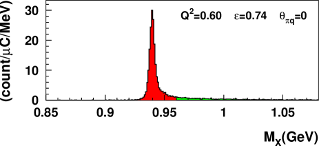
Figure 1: (Color online) Representative missing mass distribution. Cuts at 0.925 and 0.960 GeV were applied to select the recoil neutron final state.

The data analysis is an updated version of that in Ref. vol01 . First, experimental yields were determined. Electrons in the SOS were identified by using the combination of a lead glass calorimeter and gas C̆erenkov detector. Pion identification in the HMS was accomplished by requiring no signal in a gas C̆erenkov detector and by using time of flight between two scintillator hodoscope planes. The momenta of the scattered electron and the pion at the target vertex were reconstructed from the wire chamber information of the spectrometers, correcting for energy loss in the target. From these, the values of $Q^{2}$, $W$, $t$, and the missing mass were reconstructed. A cut on the latter of 0.925 to 0.96 GeV was used to select the neutron exclusive final state, excluding additional pion production (Fig. 1). Experimental yields as function of $Q^{2}$, $W$, $t$ and $\phi$ were then determined by subtracting random coincidences (varying with bin but typically 1.2%) and aluminum target window contributions (typically 0.6%) and correcting for trigger, tracking and particle-identification efficiencies, pion absorption, local target-density reduction due to beam heating, and dead times. Details of these procedures are similar to those found in Ref. thesis .

Cross sections were obtained from the yields using a detailed Monte Carlo (MC) simulation of the experiment, which included the magnets, apertures, detector geometries, realistic wire chamber resolutions, multiple scattering in all materials, optical matrix elements to reconstruct the particle momenta at the target from the information of the wire-chambers of the spectrometers, pion decay (including misidentification of the decay muon as a pion), and internal and external radiative processes.

Calibrations with the over-determined ¹H$(e,e^{\prime}p)$ reaction were instrumental in various applications. The beam momentum and the spectrometer central momenta were determined absolutely to better than 0.1%, while the incident beam angle and spectrometer central angles were determined with an absolute accuracy of about 0.5 mrad. The spectrometer acceptances were checked by comparison of the data to the MC simulations. Finally, the overall absolute cross section normalization was checked. The calculated yields for $e+p$ elastics agreed to better than 2% with predictions based on a parameterization of the world data bos95 .

In the pion production reaction, the experimental acceptances in $W$, $Q^{2}$ and $t$ are correlated. By using a realistic cross section model in the MC simulation, possible errors resulting from averaging the measured yields when calculating cross sections at average values of $W$, $Q^{2}$ and $t$, can be minimized. A phenomenological cross section model was obtained (see below) by fitting the different cross sections $\sigma_{X}$ of Eqn. (4) globally to the data as a function of $Q^{2}$ and $t$ in the whole range of $Q^{2}$. The dependence of the cross section on $W$ was assumed to follow the phase space factor $(W^{2}-M^{2}_{p})^{-2}$, which is supported by previous data bra79 .

The experimental cross sections can then be calculated from the measured and simulated yields via the relation

$$\left(\frac{d\sigma(\overline{W},{\overline{Q}}^{2},t,\phi)}{dt}\right)_{\mathrm{exp}}=\frac{\langle Y_{\mathrm{exp}}\rangle}{\langle Y_{\mathrm{MC}}\rangle}\left(\frac{d\sigma(\overline{W},{\overline{Q}}^{2},t,\phi)}{dt}\right)_{\mathrm{MC}}.$$ (5)

This was done for five bins in $t$ at each of the four $Q^{2}$-values. Here, $\langle Y\rangle$ indicates that the yields were averaged over the $W$ and $Q^{2}$ acceptance, $\overline{W}$ and $\overline{Q}^{2}$ being the acceptance (of high and low $\epsilon$ together) weighted average values for that $t$-bin. By using these average values, possible errors due to extrapolating the MC model cross section used to outside the region of the experimental data, is avoided.

Figure 2: Example of the measured cross sections, $\frac{d^{2}\sigma}{dtd\phi}$ as a function of $\phi$ at $Q^{2}$=0.6 GeV² for two values of $\epsilon$. The curves shown represent the model cross section used in the Monte Carlo simulation.

By combining for every $t$-bin (and for the four values of $Q^{2}$) the $\phi$-dependent cross sections measured at two values of the incoming electron energy, and thus of $\epsilon$, the experimental values of $\sigma_{\mathrm{L}}$, $\sigma_{\mathrm{T}}$, $\sigma_{\mathrm{LT}}$ and $\sigma_{\mathrm{TT}}$ can be determined by fitting the $\phi$ and $\epsilon$-dependence (Fig. 2). In this fit, the leading order $\sin\theta$ ($\sin^{2}\theta$) of $\sigma_{\mathrm{LT}}$($\sigma_{\mathrm{TT}}$), where $\theta$ is the angle between the three-momentum transfer and the direction of the outgoing pion, was taken into account. Those values were then used to improve upon the model cross section used in the MC simulation. This whole procedure was iterated until the values of $\sigma_{\mathrm{L}}$, $\sigma_{\mathrm{T}}$, $\sigma_{\mathrm{LT}}$ and $\sigma_{\mathrm{TT}}$ converged. The dependence of $\sigma_{L}$ (and $\sigma_{T}$) on the MC input model was small (see below).

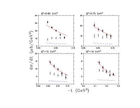
Figure 3: (Color online) Separated cross sections $\sigma_{\mathrm{L}}$ [solid] and $\sigma_{\mathrm{T}}$ [open]. The error bars represent the combination of statistical and $t$ uncorrelated systematic uncertainties. In addition, there is an overall systematic uncertainty of about 6%, mainly from the $t$ correlated, $\epsilon$ uncorrelated systematic uncertainty. The solid and dashed curves denote VGL model calculations for $\sigma_{\mathrm{L}}$ and $\sigma_{\mathrm{T}}$ with parameters $\Lambda^{2}_{\pi}$=0.393, 0.373, 0.412, 0.458 GeV²for $Q^{2}$=0.6-1.6 GeV², and with common $\Lambda^{2}_{\rho}$=1.5 GeV². The discontinuities in the curves result from the different average $\overline{W}$ and ${\overline{Q}}^{2}$ of each $t$-bin.

The separated cross sections $\sigma_{\mathrm{L}}$ and $\sigma_{\mathrm{T}}$ are shown in Fig. 3. They are presented as differential cross sections $d\sigma/dt$ as a function of $t$, at the center of the $t$-bin. The longitudinal cross section exhibits the expected $t$-pole behavior. The transverse cross section is mostly flat.

The total uncertainty in the experimental cross sections is a combination of statistical and systematic uncertainties. All contributions to the systematic uncertainty were carefully investigated, also using the results of extensive single-arm L/T separation experiments and of ¹H$(e,e^{\prime}p)$ calibration reactions in Hall C chr04 . The experimental systematic uncertainties include contributions that, like the statistical uncertainties, are uncorrelated between the measurements at the two $\epsilon$ values, and others that are correlated. Most of the uncorrelated ones are common to all $t$ bins, but there is a small contribution, estimated as 0.7%, that is also uncorrelated in $t$. The $\epsilon$-uncorrelated uncertainties in $\sigma_{\mathrm{L}}$ are inflated by the factor $1/\Delta\epsilon$ in the L/T separation, where $\Delta\epsilon$ is the difference (typically 0.3) in the photon polarization between the two measurements. The effect on $\sigma_{\mathrm{T}}$ depends on the exact $\epsilon$ values. The $\epsilon$-uncorrelated systematic uncertainty in the unseparated cross sections common for all $t$-bins was estimated to be 1.7%, while the total correlated uncertainty is 2.8-4.1%, depending on $t$. Apart from a dependence of the separated cross sections on the MC model used, which ranges from 0.2% to a maximum of 3% for one highest $t$-bin, the largest contributions are: the detection volume (1.5%), dependence of the extracted cross sections on the momentum and angle calibration (1%), target density (1%), pion absorption (1.5%), pion decay (1%), the simulation of radiative processes (1.5%), and detector efficiency corrections (1%). The overall uncertainty is slightly smaller than used in Ref. vol01 .

Figure 4: Differential cross section comparison between our earlier $Q^{2}$=0.75 GeV² results [open circles] (Ref. vol01 ) and this work [filled circles]. The unseparated cross sections ($\sigma_{uns}=\epsilon\sigma_{L}+\sigma_{T}$) at high and low $\epsilon$ are nearly identical, but the differences between the separated $\sigma_{\mathrm{L}}$ and $\sigma_{\mathrm{T}}$ are somewhat larger. The $\sigma_{uns}$ error bars include the statistical and epsilon uncorrelated systematics only and are in many cases smaller than the plotting symbols. Those for $\sigma_{L,T}$ include the contribution of all statistical and systematic uncertainties.

$\overline{Q^{2}}$	$\overline{W}$	$-t$	$d\sigma_{L}/dt$	$d\sigma_{T}/dt$
(GeV2)	(GeV)	(GeV2)	($\mu$b/GeV2)	($\mu$b/GeV2)
0.526	1.983	0.026	31.360 $\pm$ 1.602, 1.927	8.672 $\pm$ 1.241
0.576	1.956	0.038	24.410 $\pm$ 1.119, 1.774	10.660 $\pm$ 1.081
0.612	1.942	0.050	20.240 $\pm$ 1.044, 1.583	10.520 $\pm$ 1.000
0.631	1.934	0.062	14.870 $\pm$ 1.155, 1.366	10.820 $\pm$ 0.992
0.646	1.929	0.074	11.230 $\pm$ 1.469, 1.210	10.770 $\pm$ 1.097
0.660	1.992	0.037	20.600 $\pm$ 1.976, 1.895	9.812 $\pm$ 1.532
0.707	1.961	0.051	16.280 $\pm$ 1.509, 1.788	10.440 $\pm$ 1.344
0.753	1.943	0.065	14.990 $\pm$ 1.270, 1.573	8.580 $\pm$ 1.150
0.781	1.930	0.079	11.170 $\pm$ 1.214, 1.416	9.084 $\pm$ 1.091
0.794	1.926	0.093	9.949 $\pm$ 1.376, 1.277	8.267 $\pm$ 1.110
0.877	1.999	0.060	14.280 $\pm$ 1.157, 1.103	7.084 $\pm$ 0.791
0.945	1.970	0.080	11.840 $\pm$ 0.887, 0.978	6.526 $\pm$ 0.657
1.010	1.943	0.100	9.732 $\pm$ 0.773, 0.837	5.656 $\pm$ 0.572
1.050	1.926	0.120	7.116 $\pm$ 0.789, 0.747	5.926 $\pm$ 0.570
1.067	1.921	0.140	4.207 $\pm$ 1.012, 0.612	5.802 $\pm$ 0.656
1.455	2.001	0.135	5.618 $\pm$ 0.431, 0.442	3.613 $\pm$ 0.294
1.532	1.975	0.165	4.378 $\pm$ 0.356, 0.390	3.507 $\pm$ 0.257
1.610	1.944	0.195	3.191 $\pm$ 0.322, 0.351	3.528 $\pm$ 0.241
1.664	1.924	0.225	2.357 $\pm$ 0.313, 0.310	3.354 $\pm$ 0.228
1.702	1.911	0.255	2.563 $\pm$ 0.356, 0.268	2.542 $\pm$ 0.227

Table 1: Separated cross sections $\sigma_{\mathrm{L}}$ and $\sigma_{\mathrm{T}}$ from this work. The two listed uncertainties for $\sigma_{\mathrm{L}}$ are the combination of statistical and $t$-uncorrelated systematic uncertainties, and the combination of the $\epsilon$-correlated and uncorrelated uncertainties. The statistical and $t$-uncorrelated uncertainties are applied before fitting the VGL model to the data, while the $\epsilon$-correlated and uncorrelated uncertainties are applied afterwards. The listed errors for $\sigma_{\mathrm{T}}$ include all experimental uncertainties.

The unseparated cross sections and hence also the values of $\sigma_{\mathrm{L}}$ and $\sigma_{\mathrm{T}}$ of the present analysis differ from those of our earlier analysis presented in Ref. vol01 . Compared to that analysis, small adjustments were made in the values of cuts and efficiencies. Also, a small mistake was found in calculating the value of $\theta$, which affects the calculation of the cross section in Eqn. 5. Finally, as mentioned, the method to separate the cross sections was changed. The cross sections in Table 1 are our final values. Except for a few cases, the difference with the previous values is well within the total uncertainty quoted in Ref. vol01 . As an example, the old and the new cross sections for the case $Q^{2}$= 0.75 GeV² are shown in Fig. 4. It can be seen that the differences in the extracted unseparated cross sections (top panels) are very small, but the L/T separation increases them. On average over the four $Q^{2}$ cases, $\sigma_{\mathrm{L}}$ is 6% smaller than in Ref. vol01 and $\sigma_{\mathrm{T}}$ is 3% larger. The largest differences occur for $Q^{2}$=1.0 GeV², where $\sigma_{\mathrm{L}}$ is 14% smaller and $\sigma_{\mathrm{T}}$ is 10% larger.

III Extraction of $\bf F_{\pi}(Q^{2})$ from the Data

It should be clear that the differential cross sections $\sigma_{\mathrm{L}}$ versus $t$ over some range of $Q^{2}$ and $W$ are the actual observables measured by the experiment. The extraction of the pion form factor from these cross sections can be done in a number of approaches, each with their own merits and associated uncertainties.

Frazer frazer originally proposed that $F_{\pi}$ be extracted from $\sigma_{\mathrm{L}}$ via a kinematic extrapolation to the pion pole, and that this be done in an analytical manner, à la Chew-Low chew . This extrapolation procedure fails to produce a reliable answer, since different polynomial fits, each of which are equally likely in the physical region, differ considerably when continued to $t=m_{\pi}^{2}$. Some attempts were made kellett to reduce this uncertainty by providing some theoretical constraints on the behavior of the pion form factor in the unphysical region, but none proved adequate.

Bebek et al. beb78 embraced the use of theoretical input when they used the Born term model of Berends berends to perform a form factor determination. Brauel et al. bra79 similarly used the Born term model of Gutbrod and Kramer gut72 to extract $F_{\pi}$. The presence of the nucleon and its structure complicates the theoretical model used, and so an unavoidable implication of this method is that the extraction of the pion form factor becomes model dependent.

As in Ref. vol01 ; hor06 , the Regge model by Vanderhaeghen, Guidal and Laget (VGL, Ref. van97 ) is used here to extract $F_{\pi}$. In this model, the pole-like propagators of Born term models are replaced with Regge propagators, and so the interaction is effectively described by the exchange of a family of particles with the same quantum numbers instead of the exchange of one particle. The model was first applied to pion photoproduction. Most of the model’s free parameters were determined from data on nucleon resonances. The use of Regge propagators, and the fact that both the $\pi$ ($J=0$) and the $\rho$ ($J=1$) trajectories are incorporated in the model proved to be essential to obtain a good description of the $W$- and $t$-dependence of the photoproduction data for both $\pi^{+}$ and $\pi^{-}$ particles. For electroproduction, the pion form factor and the $\rho\pi\gamma$ form factor are added as adjustable parameters, parameterized with a monopole form

$$F_{\pi}(Q^{2})=[1+Q^{2}/\Lambda^{2}_{\pi}]^{-1}.$$ (6)

The Regge model does a superior job of describing the $t$ dependence of the differential pion electroproduction cross sections of bra79 ; ack78 than the Born term model. Over the range of $-t$ covered by this work, $\sigma_{\mathrm{L}}$ is completely determined by the $\pi$ trajectory, whereas $\sigma_{\mathrm{T}}$ is also sensitive to the $\rho$ exchange contribution. The value of $\Lambda^{2}_{\rho}$ is poorly known, while $\Lambda^{2}_{\pi}$ is much better known and in the end is determined by the fitting of the model to the $\sigma_{\mathrm{L}}$ data.

The VGL model for certain choices of $\Lambda^{2}_{\pi}$ and $\Lambda^{2}_{\rho}$ is compared to our data in Figure 3. The VGL cross sections have been evaluated at the same $\overline{W}$ and $\overline{Q^{2}}$ values as the data, resulting in the discontinuities shown. The model strongly underestimates $\sigma_{\mathrm{T}}$ for any value of $\Lambda^{2}_{\rho}$ used (variation of $\Lambda^{2}_{\rho}$ within reasonable values can change $\sigma_{\mathrm{T}}$ by up to 40%). Since the JLab data have been taken at relatively low values of $W\approx 1.95$ GeV, this may be due to contributions from resonances, enhancing the strength in $\sigma_{\mathrm{T}}$. No such terms are included explicitly in the Regge model. The VGL model calculation for $\sigma_{\mathrm{L}}$ gives the right magnitude, but the $t$ dependence of the data is somewhat steeper than that of the calculations. This is most visible at $Q^{2}$=0.6 GeV². As in the case of $\sigma_{\mathrm{T}}$, the discrepancy between the data and VGL is attributed to resonance contributions. This is supported by the fact that the discrepancy is strongest at the lowest $Q^{2}$ value, at higher $Q^{2}$ the resonance form factor reduces such contributions.

Given this discrepancy in shape between the VGL calculations and the $\sigma_{\mathrm{L}}$ data, the questions are: 1) how to determine the value of $F_{\pi}$ from the measured longitudinal cross sections $\sigma_{\mathrm{L}}$, and 2) what is the associated ‘model uncertainty’ in doing so? The difficulty is that there is no theoretical guidance for the assumed interfering background. This applies even if one assumes that the background is due to resonances: virtually nothing is known about the L/T character of resonances at $W=1.95$ GeV, let alone their influence on $\sigma_{\mathrm{L}}$ (via interference with the VGL amplitude).

III.1 Summary of our Previous Extraction Method

In our previous analysis vol01 , the following procedure was adopted. When fitting the value of $\Lambda^{2}_{\pi}$ (and hence $F_{\pi}$) for the separate $t$-bins the value of $\Lambda^{2}_{\pi}$ increases when $-t$ decreases, since the data are steeper in $|t|$ than the VGL calculations. The value of $F_{\pi}$ extracted from the lowest $|t|$-bin, which is closest to the pole, was thus taken as a lower limit.

An upper limit for $F_{\pi}$ was obtained by assuming that the background effectively yields a constant negative contribution to $\sigma_{\mathrm{L}}$. This background and the value of $\Lambda^{2}_{\pi}$ were then fitted together, assuming that the background is constant with $t$. The fitted contribution of the background was found to drop strongly as $Q^{2}$ increased from 0.6 to 1.6 GeV². Since in $\sigma_{\mathrm{T}}$ this ‘missing background’ (i.e. the difference between the data and VGL model) decreases, at least for $Q^{2}$=0.6 GeV², with decreasing $-t$ (Fig. 3), and assuming that this also holds for $\sigma_{\mathrm{L}}$, these assumptions give an upper estimate for $F_{\pi}$. The best estimate for $F_{\pi}$ was then taken as the average of the two results and one half of the average of the (relative) differences was taken as the ‘model uncertainty’.

However, the asumptions made in this procedure may be questioned. Firstly, the value of $F_{\pi}$ extracted from the lowest $|t|$-bin does not have to be a lower limit, and secondly, the assumption of a negative interfering $t$-independent cross section in the upper limit calculation requires a special magnitude and phase for the interfering amplitude with respect to the VGL amplitude.

III.2 Another Form Factor Extraction Method

Since the publication of those results, we have looked at the discrepancy between the $t$-dependence predicted by the VGL model and the data in more detail by assuming, besides the VGL amplitude, a $t$-independent interfering background amplitude, and fitting the latter together with the value of $\Lambda^{2}_{\pi}$. The fitting uncertainty in $\Lambda^{2}_{\pi}$ varies between 5% and 18%, while the magnitude and phase of the fit background amplitude are very poorly constrained (uncertainties in the hundreds of percent).

Although the fitting uncertainties are very large, the results of this exercise suggest an interfering amplitude whose magnitude decreases monotonically with increasing $Q^{2}$, but whose phase with respect to the VGL amplitude does not necessarily result in a net negative cross section contribution to $\sigma_{\mathrm{L}}$, as has been assumed in the previous analysis. However, here also a special assumption was used, i.e. an interfering amplitude with a magnitude and phase that do not depend on $t$. Thus, determining $F_{\pi}$ in this way is not a viable method, either.

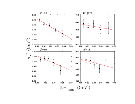
Figure 5: (Color online) Values of $\Lambda^{2}_{\pi}$ determined from the fit of the VGL model to each $t$-bin, and linear fit to same. The error bars reflect the statistical and $t$-uncorrelated systematic uncertainties. The additional overall systematic uncertainties, which are applied after the fit, are not shown.

III.3 Adopted Form Factor Extraction Method

Given that no information is available on the background, we are forced to make some assumptions in extracting $F_{\pi}$ from these data. Our guiding principle is to minimize these assumptions to the greatest extent possible. The form factor extraction method that we have adopted relies on the single assumption, that the contribution of the background is smallest at the kinematic endpoint $t_{min}$.

$Q^{2}$	W	$\Lambda^{2}_{\pi}$	$F_{\pi}$
(GeV2)	(GeV)	(GeV2)
0.60	1.95	$0.458\pm 0.031^{+0.255}_{-0.068}$	$0.433\pm 0.017^{+0.137}_{-0.036}$
0.75	1.95	$0.388\pm 0.038^{+0.135}_{-0.053}$	$0.341\pm 0.022^{+0.078}_{-0.031}$
1.00	1.95	$0.454\pm 0.034^{+0.075}_{-0.040}$	$0.312\pm 0.016^{+0.035}_{-0.019}$
1.60	1.95	$0.485\pm 0.038^{+0.035}_{-0.027}$	$0.233\pm 0.014^{+0.013}_{-0.010}$
0.70	2.19	$0.627\pm 0.058^{+0.096}_{-0.085}$	$0.473\pm 0.023^{+0.038}_{-0.034}$

Table 2: $\Lambda^{2}_{\pi}$ and $F_{\pi}$ values from this work, and the reanalyzed data from Ref. bra79 using the same method. The first error includes all experimental and analysis uncertainties, and the second error is the ‘model uncertainty’ as described in the text.

Our best estimate for $F_{\pi}$ is thus determined in the following manner. Using the value of $\Lambda^{2}_{\pi}$ as a free parameter, the VGL model was fitted to each $t$-bin separately, yielding $\Lambda^{2}_{\pi}(\overline{Q^{2}},\overline{W},t)$ values as shown in Fig. 5. The values of $\Lambda^{2}_{\pi}$ tend to decrease as $-t$ increases, presumably because of an interfering background not included in the model. Since the pole cross section containing $F_{\pi}$ increases strongly with decreasing $-t$, and the background presumably remains approximately constant, as suggested by the difference between data and VGL calculations for $\sigma_{\mathrm{T}}$, we assume that the effect of this background will be smallest at the smallest value of $|t|$ allowed by the experimental kinematics, $|t_{min}|$. Thus, an extrapolation of $\Lambda^{2}_{\pi}$ to this physical limit is used to obtain our best estimate of $F_{\pi}$. The value of $\Lambda^{2}_{\pi}$ at $t_{min}$ is obtained by a linear fit to the data in Fig. 5. The resulting $\Lambda^{2}_{\pi}$ and $F_{\pi}$ values are listed in Table 2. The first uncertainty given represents both the experimental and the linear fit extrapolation uncertainties.

The $F_{\pi}$ values listed in Table 2 correspond to the true values within the context of the VGL model if, and only if, the background vanishes at $|t-t_{min}|=0$. Because of the uncertainty inherent in this assumption, we also estimate a ‘model uncertainty’ to account for the possible influence of the missing ingredient in the VGL model (background) at $|t-t_{min}|=0$. Lacking a model for the background, we can only try to make a fair estimate of this uncertainty. This was done by looking at the variation in the fitted values of $\Lambda^{2}_{\pi}$ when using two different assumptions for the background. We used the two cases considered earlier in this paper when trying to determine $F_{\pi}$. The first case assumes the $t$-independent negative background in addition to the VGL model used in Sec. III.1. The second case assumes the interfering background amplitude with a $t$-independent magnitude and phase discussed in Sec. III.2. However, here they are not used to determine $F_{\pi}$, but only to estimate the model uncertainty in our best value of $F_{\pi}$ determined above.

The estimated model uncertainty is determined from the spread of the $\Lambda^{2}_{\pi}$ values at each $Q^{2}$ given by these two methods. Each effectively represents a different background interference with the VGL model. To keep the number of degrees of freedom the same in all cases, the background was fixed to the minimum $\chi^{2}$ value determined in each of the above two studies, and $\Lambda^{2}_{\pi}$ and its uncertainty was then determined in a one-parameter fit of the VGL model plus background to the $\sigma_{\mathrm{L}}$ data. Since there is a strong statistical overlap between the two fits, the statistical plus random uncertainties of the data were quadratically removed from the $\Lambda^{2}_{\pi}$ uncertainties. The model uncertainty at each $Q^{2}$ is then assigned to be the range plus fitting uncertainty given by the two methods, relative to the value of $\Lambda^{2}_{\pi}$ at $t_{min}$. The resulting (asymmetric) uncertainties are listed as the second uncertainty in Table 2.

The model uncertainty in the $F_{\pi}$ value drops from about 20% at $Q^{2}$=0.6 GeV² to about 5% at 1.6 GeV². This is consistent with the fact that the discrepancy with the $t$-dependence of the VGL calculation is smaller for the larger values of $Q^{2}$. It is also at least compatible with the idea that resonance contributions, which presumably have a form factor that drops fast with $Q^{2}$, are responsible. The corresponding model uncertainty quoted in Ref. vol01 was approximately 8.5% at all $Q^{2}$, but that was based on a more restrictive assumption on the background (in essence case 1).

IV Results and Discussion

Because of the arguments given above, the values presented in Table 2 and Fig. 6 are our final estimate of $F_{\pi}$ from these data using this model. However, we stress that the primordial results of our experiment are the $\sigma_{\mathrm{L}}$ cross sections. When improved models for the ¹H$(e,e^{\prime}\pi^{+})n$ reaction become available, other (better) values of $F_{\pi}$ may be extracted from the same cross sections.

The present values for $F_{\pi}$ are between 7% and 16% smaller than our previously published values vol01 , which is about the combined experimental and model uncertainty. The largest difference is at $Q^{2}=0.75$ GeV². On average, one quarter of the difference is because the final values of $\sigma_{\mathrm{L}}$ are smaller than those of Ref. vol01 (see Fig. 4 for a representative comparison), and the remaining three quarters are due to the $F_{\pi}$ extraction method, the present method being closer to the method used in Ref. vol01 to obtain the lower limit.

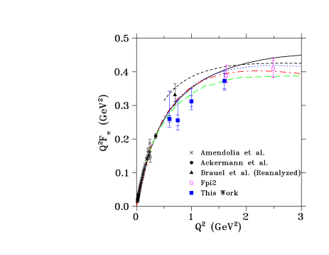
Figure 6: (Color online) $Q^{2}F_{\pi}$ data from this work, compared to previously published data. The Brauel et al. bra79 point has been reanalyzed using the $F_{\pi}$ extraction method of this work. The outer error bars for this work and the reanalyzed Brauel et al. data include all experimental and model uncertainties, added in quadrature, while the inner error bars reflect the experimental uncertainties only. Also shown are the light front quark model hwa01 (dash-dot), Dyson-Schwinger mar00 (solid), QCD sum-rule nes82 (dot), dispersion relation ges00 (long-dash), and quark-hadron duality mel03 (short-dash), calculations.

Analyses of other data at higher $W$ indicate that the discrepancy with the $t$-dependence of the VGL calculation is much smaller at higher values of $W$. The data from Brauel et al. bra79 , taken at $Q^{2}$=0.70 GeV² and a value of $W$=2.19 GeV, were reanalyzed using the $F_{\pi}$ extraction method presented here. The result is 0.4% higher than that obtained using the $F_{\pi}$ extraction method of Ref. vol01 . This indicates that our $F_{\pi}$ extraction methods are robust when the background contribution is small, as appears to be the case at this higher value of $W$.

The data from our second experiment hor06 at $W$=2.22 GeV and $Q^{2}$=1.6, 2.45 GeV² are also shown in Fig. 6. There, the VGL model adequately describes the $t$-dependence of the $\sigma_{\mathrm{L}}$ data, again indicating that the background contributions for $\sigma_{\mathrm{L}}$ are smaller at higher $W$, even though the model strongly underpredicts the magnitude of $\sigma_{\mathrm{T}}$. In that case, the VGL model was fit to the full $t$-range of the $\sigma_{\mathrm{L}}$ data with only small fitting uncertainties. It is seen in the figure that the revised $Q^{2}$=1.6 GeV² result from this work agrees well with that from our second experiment, taken at higher $W$ and 30% closer to the $\pi^{+}$ pole. The excellent agreement between these two results, despite their significantly different $t_{min}$ values, indicates that the uncertainties due to the $\pi^{+}$ electroproduction reaction mechanism seem to be under control, at least in this $Q^{2}$-range.

Fig. 6 compares our final data from this work and from our second experiment hor06 to several QCD-based calculations. The combined data sets are consistent with a variety of models. Up to $Q^{2}$=1.5 GeV², the Dyson-Schwinger calculation of Ref. mar00 , the light front quark model calculation of Ref. hwa01 , and the QCD sum-rule calculation of Ref. nes82 are nearly identical, and are all very close to the monopole form factor constrained by the measured pion charge radius ame86 . Such a form factor reflects non-perturbative physics. Our revised data are below the monopole curve. A significant deviation would indicate the increased role of perturbative components at moderate $Q^{2}$, which provide in that region a value of $Q^{2}F_{\pi}\approx$0.15-0.20 only bak04 . The dispersion relation calculation of Geshkenbein et al. ges00 is closer to our results in the $Q^{2}$=0.6-1.6 GeV² region, while still describing the low $Q^{2}$ data used for determining the pion charge radius. The quark-hadron duality calculation by Melnitchouk mel03 is not expected to be valid below $Q^{2}$=2.0 GeV². This is reflected in its significant deviation from the monopole curve at low $Q^{2}$. To better distinguish between these different models, it is clear that especially higher $Q^{2}$ data, as well as more data at higher values of $W$ in the $Q^{2}$=0.6-1.6 GeV² region, are needed. Plans are underway to address both of these at JLab.

V Summary and Conclusions

To summarize, the data analysis for our ¹H$(e,e^{\prime}\pi^{+})n$ experiment at $Q^{2}$=0.6-1.6 GeV², centered at $W=1.95$ GeV, has been repeated with careful inspection of all steps. The final unseparated cross sections presented here are in most cases consistent with our previous analysis within experimental uncertainties. After the magnifying effect of the L/T separation, the resulting $\sigma_{\mathrm{T}}$ values are slightly larger than before, and the $\sigma_{\mathrm{L}}$ values are correspondingly smaller. The experimental systematic uncertainties were critically reviewed, and are slightly smaller compared to the previous analysis.

As before, we use a fit of the Regge model of Ref. van97 to our $\sigma_{\mathrm{L}}$ data to extract $F_{\pi}$. The data display a steeper $t$-dependence than the model, which we attribute to the presence of longitudinal background contributions not included in the model. After revisiting our prior assumptions used to extract $F_{\pi}$ from $\sigma_{\mathrm{L}}$ with the model, we conclude that some of our prior analysis assumptions were unwarranted. Therefore, we employ a revised $F_{\pi}$ extraction method which relies only on the assumption that the background contributions are minimal at $t_{min}$. The resulting values are our best estimate of $F_{\pi}$ from these data with this model, and are between 8% and 16% smaller than before, primarily due to the different extraction method. The Brauel et al. bra79 data at similar $Q^{2}$ but higher $W$ are robust against our fitting assumptions, consistent with our expectation that a longitudinal background contribution not included in the Regge model is the cause of the discrepancy.

The new analysis, in addition to providing our final $F_{\pi}$ results for the $Q^{2}$=0.6-1.6 GeV² range, gives an indication of the contribution of the analysis assumptions to the $F_{\pi}$ determination. A detailed analysis yields model uncertainties that decrease with increasing $Q^{2}$ and $W$. They are consistent with the differences in the values of $F_{\pi}$ determined using the previous and present extraction methods. They indicate that, given the present electroproduction model, the uncertainty in the dtermination of $F_{\pi}$ in this $W$ and $Q^{2}$ range is of the order of 10%.

The revised data indicate that for $Q^{2}$$>0.5$ GeV², $F_{\pi}$ starts to fall below the monopole curve that describes the low $Q^{2}$ elastic scattering data. These results are consistent with those of our second, more precise experiment at higher $Q^{2}$and $W$ hor06 . The two sets of data at $Q^{2}=1.6$ GeV² are taken with significantly different $t_{min}$, and so if the various form factor extraction issues were not being handled well by the VGL model, a significant discrepancy would have been expected to result. Their good agreement lends further credibility to the analysis presented here. It will be useful to acquire additional electroproduction data in the $0.5<Q^{2}<1.5$ GeV² range at higher $W$ in order to be able to extract more precise values of $F_{\pi}$ without the difficulties encountered here.

VI Acknowledgments

The authors would like to thank Drs. Guidal, Laget and Vanderhaeghen for stimulating discussions and for modifying their computer program for our needs. This work is supported by DOE and NSF (USA), FOM (Netherlands), NSERC (Canada), KOSEF (South Korea), and NATO.

References

- (1) G.P. Lepage, S.J. Brodsky, Phys. Lett. 87B (1979) 359.
- (2) A.P. Bakulev et al., Phys. Rev. D 70 (2004) 033014.
- (3) B. Melic, B. Nizic, K. Passek, Phys. Rev. D 60 (1999) 074004.
- (4) A.V. Radyushkin, Nucl. Phys. A 532 (1991) 141c.
- (5) V.M. Braun, A. Khodjamirian, M. Maul, Phys. Rev. D 61 (2000) 073004.
- (6) C.-W. Hwang, Phys. Rev. D 64 (2001) 034011.
- (7) P. Maris, P.C. Tandy, Phys. Rev. C 62 (2000) 055204.
- (8) G. Sterman, P. Stoler, Ann. Rev. Nucl. Part. Sci. 47 (1997) 183.
- (9) S. R. Amendolia, et al., Nucl. Phys. B277 (1986) 168.
- (10) C. J. Bebek, et al., Phys. Rev. D 17 (1978) 1693.
- (11) H. Ackermann, et al., Nucl. Phys.B137 (1978) 294.
- (12) P. Brauel, et al., Z. Phys. C3 (1979) 101.
- (13) J. Volmer, et al., Phys. Rev. Lett. 86 (2001) 1713.
- (14) J. Volmer, PhD thesis, Vrije Universiteit, Amsterdam (2000),
- (15) P. E. Bosted, Phys. Rev. C 51 (1995) 409.
- (16) M.E. Christy, et al., Phys. Rev. C 70 (2004) 015206.
- (17) W.R. Frazer, Phys. Rev. 115 (1959) 1763.
- (18) G.F. Chew, F.E. Low, Phys. Rev. 113 (1959) 1640.
- (19) B.H. Kellett, C. Verzegnassi, Nuo. Cim. 20A (1974) 194.
- (20) F.A. Berends, Phys. Rev. D 1 (1970) 2590.
- (21) F. Gutbrod and G. Kramer, Nucl. Phys. B49 (1972) 461.
- (22) T. Horn, et al, Phys. Rev. Lett. 97 (2006) 192001.
- (23) M. Vanderhaeghen, M. Guidal and J.-M. Laget, Phys. Rev. C 57 (1998) 1454; Nucl. Phys. A627 (1997) 645.
- (24) V.A. Nesterenko, A.V. Radyushkin, Phys. Lett. 115 B (1982) 410.
- (25) B.V. Geshkenbein, Phys. Rev. D 61 (2000) 033009.
- (26) W. Melnitchouk, private communication 2006, and Eur. Phys. J. A 17 (2003) 233.