A measurement of the ⁴He$(\gamma,n)$ reaction from 23 $\bm{<}$ E$\bm{}{\gamma}$ $\bm{<}$ 70 MeV

Abstract

A comprehensive set of ⁴He$(\gamma,n)$ absolute cross-section measurements has been performed at MAX-lab in Lund, Sweden. Tagged photons from 23 $<$ $E_{\gamma}$ $<$ 70 MeV were directed toward a liquid ⁴He target, and neutrons were identified using pulse-shape discrimination and the time-of-flight technique in two liquid-scintillator detector arrays. Seven-point angular distributions have been measured for fourteen photon energies. The results have been subjected to complementary Transition-coefficient and Legendre-coefficient analyses. The results are also compared to experimental data measured at comparable photon energies as well as Recoil-Corrected Continuum Shell Model, Resonating Group Method, and Effective Interaction Hyperspherical-Harmonic Expansion calculations. For photon energies below 29 MeV, the angle-integrated data are significantly larger than the values recommended by Calarco, Berman, and Donnelly in 1983.

I Introduction

Over the past 50 years, a very large body of experimental work has been performed in order to understand the near-threshold photodisintegration of ⁴He. In 1983, Calarco, Berman, and Donnelly (CBD) assessed all of the available experimental data in a benchmark review article Calarco et al. (1983) and made a recommendation as to the value of the ⁴He$(\gamma,n)$ photodisintegration cross section from threshold up to $E_{\gamma}$ $\sim$ 50 MeV. Since then, most of the experimental effort has been directed towards measuring either the ratio of the photoproton-to-photoneutron cross sections or simply the photoproton channel. Up-to-date reviews of all available data are made in Refs. Quaglioni et al. (2004); Shima et al. (2005). In contrast to the $(\gamma,p)$ situation, only three near-threshold measurements of the photoneutron channel have to our knowledge been published Komar et al. (1993); Shima et al. (2001, 2005).

In this Paper, we present a comprehensive new data set for the ⁴He$(\gamma,n)$ reaction near threshold which has been obtained using tagged photons with energies from 23 $<$ $E_{\gamma}$ $<$ 70 MeV. We compare our data with the CBD evaluation as well as the post-CBD data. We also report the results of Transition-coefficient and Legendre-coefficient analyses of our data, and compare them to Recoil-Corrected Continuum Shell Model (RCCSM) calculations Halderson and Philpott (1981); Halderson (2004), a Resonating Group Method (RGM) calculation Wachter et al. (1988), and an Effective Interaction Hyperspherical Harmonic (EIHH) Expansion calculation Quaglioni et al. (2004). A detailed description of the experiment is presented in Ref. Nilsson (2003), and preliminary findings have been sketched in Refs. Sims et al. (1998); Nilsson et al. (2005).

II Experiment

The experiment was performed at the tagged-photon facility Adler et al. (1997) located at MAX-lab max , in Lund, Sweden. A pulse-stretched electron beam with an energy of $\sim$93 MeV, a current of $\sim$30 nA, and a duty factor of $\sim$75% was used to produce quasi-monoenergetic photons via the bremsstrahlung-tagging technique Adler et al. (1990). A diagram of the experimental layout is shown in Figure 1.

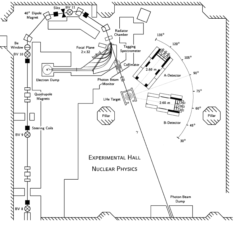
Figure 1: The photonuclear hall at MAX-lab at the time of the experiment. The electron beam passed through a 0.1% radiation-length Al radiator generating bremsstrahlung. Non-interacting electrons were dumped. Recoil electrons were momentum-analyzed using a magnetic tagging spectrometer equipped with a 64-counter focal-plane scintillator array. The resulting tagged-photon beam was collimated before it struck the storage-cell liquid-⁴He target (see Figure 2). Knocked-out neutrons were detected in two movable, large solid-angle, liquid-scintillator arrays (see Figure 3). See text for further details.

II.1 Photon beam

A 0.1% radiation-length aluminum radiator was used to convert the incident electron beam into bremsstrahlung. Non-radiating electrons were dumped into a Faraday cup which recorded the electron-beam current. This cup was surrounded by borated water, lead, and concrete shielding. Post-bremsstrahlung electrons were momentum-analyzed using a magnetic spectrometer equipped with a 64-counter focal-plane scintillator array. The photon-energy resolution of $\sim$300 keV resulted almost entirely from the 10 mm width of a single focal-plane counter. The scintillators were mounted in two 32-counter modules, and photon-energy ranges were selected by sliding the array to the appropriate position along the focal plane of the spectrometer. The average single-counter rate during these measurements was 0.5 MHz.

The size of the photon beam was defined by a tapered tungsten-alloy primary collimator. The primary collimator was followed by a dipole magnet and a post-collimator which were used to “scrub” any charged particles produced in the primary collimator. The photon-beam intensity was monitored continuously using a crude pair spectrometer which consisted of an array of three 0.5 mm thick plastic scintillators. The position of the photon beam at the target location was determined by irradiating Polaroid film after every adjustment of the electron beam. The beam spot was typically 2 cm in diameter at this position.

The tagging efficiency Adler et al. (1997) is the ratio of the number of tagged photons which struck the target to the number of recoil electrons which were registered by the associated focal-plane counter. It was measured both absolutely (using a 100% efficient lead/scintillating-fiber photon detector) and relatively (using the pair-spectrometer beam monitor) during the experiment. The absolute measurements required a very low intensity photon beam to avoid pileup in the photon detector, and were performed periodically throughout the experiment. The relative measurement was made continuously. Tagging efficiency was typically $\sim$25%.

II.2 Cryogenic target

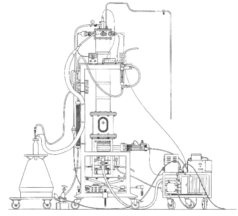
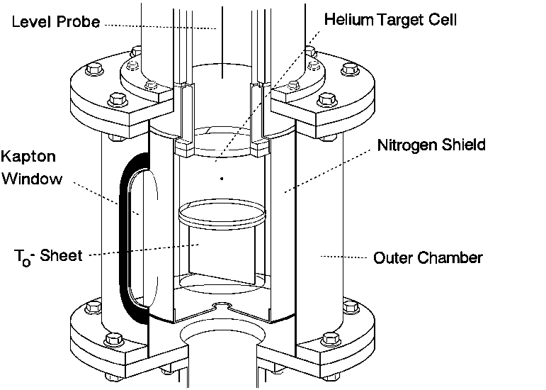
Figure 2: The cryogenic target. The top panel shows the entire cryogenic target system (including the vacuum pumps and the filling, monitoring, and support subsystems), while the bottom panel shows just the target chamber, in which two target cells were stacked vertically on top of one another. The upper cell contained the liquid ⁴He and was also used for the empty-target measurements, while the lower cell contained the 1 mm thick steel sheet used for TOF calibration of the neutron detectors. The cells could be moved in and out of the photon beam in the laboratory vertical direction using a ladder mechanism. See text for further details.

Liquid ⁴He was provided by a 6 liter, top-loaded, storage-cell cryostat Nilsson (2003), which was refilled on a $\sim$24 hour basis. The cylindrical target cell (see Figure 2) was made of 80 $\mu$m thick Kapton foil, and had a diameter of 90 mm and a height of 75 mm. It was mounted with the cylinder axis perpendicular to the direction of the photon beam and the reaction plane. The level of the liquid ⁴He in the cryostat was continuously monitored throughout the experiment by measuring the resistance of a superconducting NbTi probe. Radiative heating of the target cell was reduced using a heat shield of three layers of 30 $\mu$m thick Al foil and about ten layers of the super-insulation NRC-2, all maintained at liquid-N₂ temperature. The assembly sat in a 2 mm thick stainless-steel vacuum chamber with 125 $\mu$m thick Kapton entrance and exit windows. Vacuum was maintained using a water-cooled double-flow turbomolecular pump. The vacuum pressure in the target dewar zones was about 2 $\times$ 10^-7 mbar, which was well below the critical accomodation pressure Nilsson (2003) of 4.4 $\times$ 10^-6 mbar. Density fluctuations in the liquid ⁴He were inferred from the rate of evaporation Tate and Sadler (1983). This was monitored continuously using both the superconducting level probe and a gas-flow meter which measured the rate of outgassing of the evaporating ⁴He. The flow-rate fluctuations were negligible Nilsson (a), so that the density of the liquid helium employed in the experiment was 125.20 mg/cm³ $\pm$ 0.01%.

Empty target-cell measurements were used to determine the non-⁴He background, which was negligible. A 1 mm thick steel sheet mounted below the cell on the movable target ladder was used to convert photons to relativistic $e^{+}e^{-}$ pairs for TOF calibration of the neutron detectors (see below).

II.3 Neutron detectors

II.3.1 General properties

Neutrons were detected in two large solid-angle neutron detectors Annand et al. (1997). Each detector consisted of a 3 $\times$ 3 array of 9 rectangular cells with internal dimensions 20 cm $\times$ 20 cm $\times$ 10 cm (deep) filled with the liquid scintillator NE213A. Each cell was instrumented with a 5” photomultiplier (model 9823) from Thorn EMI. The arrays were mounted on movable platforms (30 $\deg$ $<$ $\theta_{\rm neutron}$ $<$ 135 $\deg$) and encased in Pb, steel, and borated-wax shielding. Plastic scintillators which were 65 cm $\times$ 65 cm $\times$ 2 cm (thick) were placed in front of the arrays and used to identify and veto incident charged particles. Each of the veto scintillator paddles was instrumented with two 2” photomultipliers (model XP2262B) from Philips. Since only moderate energy resolution was necessary to identify the two-body photodisintegration of ⁴He unambiguously, the detectors were placed $\sim$2.6 m (a relatively short flight path) from the target. The resulting nominal geometrical solid angle subtended by a single cell within the array was $\sim$6 msr.

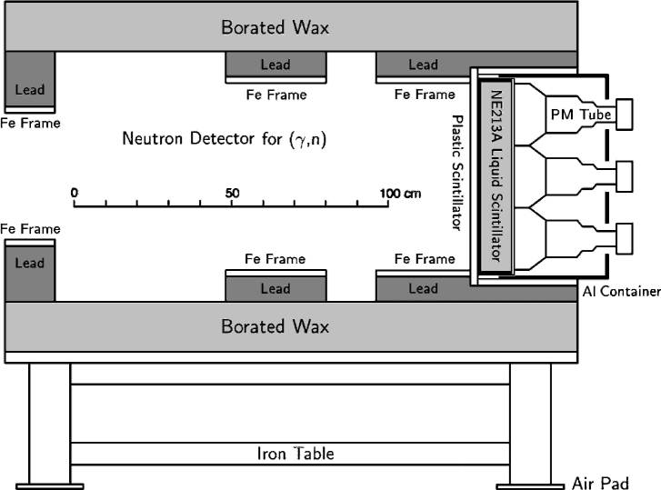
Figure 3: A sideview of one of the neutron detectors. The 9-cell detector array together with the plastic-scintillator veto and the associated shielding sat on table which could be moved using airpads. See text for further details.

II.3.2 Pulse-shape discrimination (PSD)

The PSD technique was employed in this experiment to distinguish between neutrons and photons. This technique relies on the fact that the shape of the scintillation pulse in the NE213A scintillator is dramatically different for neutrons and photons. The scintillation pulse from NE213A has both fast ($<$5 ns) and slow ($\sim$500 ns) decay components whose relative intensities depend upon the density of the ionization along the track of the interacting particle. Highly ionizing, non-relativistic protons from neutron-induced reactions in the liquid scintillator have an enhanced slow-decay intensity compared to electrons resulting from photon conversion. The total charges resulting from pulse-integration periods of 25 and 500 ns were compared using purpose-built hardware Annand (1987) which provided both a comparison (difference) analog output (the “pulse-shape” or “PS” signal) and a logic output which signaled that the comparison voltage-level threshold had been crossed. The latter was used in the hardware event trigger.

II.3.3 Time-of-flight (TOF) technique

The TOF technique was employed to determine the neutron energy. The principles of this technique are demonstrated in Figure 4. In the top panel, the tagged photon knocks a neutron out of the liquid-⁴He target cell at time $T_{0}$. This neutron is subsequently detected in a neutron-detector cell located a distance $D$ from the target at time $t_{n}$. The neutron-detector signal is used to start a time-to-digital converter (TDC), which is then stopped by the signal from the recoil electron striking the tagger focal plane. The TDC thus measures the neutron TOF ($\Delta t_{n}$) from which the neutron kinetic energy $T_{n}$ is obtained. In the bottom panel, a typical TOF spectrum is shown for neutrons of approximate energies 2.5 $<$ $T_{n}$ $<$ 6.5 MeV, which are displayed as the shaded bump. The width of this bump results from the neutron-energy range, the flight-path uncertainty, and any electronic pick-off uncertainty. The “photon” calibration peak labeled $T_{\gamma}$ lying between the neutrons and the $T_{0}$ position is much narrower, reflecting the lack of any velocity-dependent broadening. Often referred to as the “gamma flash”, it results in principle from a TOF measurement of the photons originating in the target which made it past the hardware PSD (see Section II.4). This “light-speed” peak is a useful calibration point from which $T_{0}$ can be calculated. For measurement purposes, it was enhanced by switching the plastic veto detectors in front of the neutron arrays to coincidence mode so that relativistic electrons produced in the target were also registerd. A full-width-at-half-maximum TOF neutron-energy resolution of better than 2 MeV for all photon energies was obtained in this experiment. Further, as a result of the two-body kinematics, the measured energy of the neutrons provided a cross check upon the tagged-photon energy.

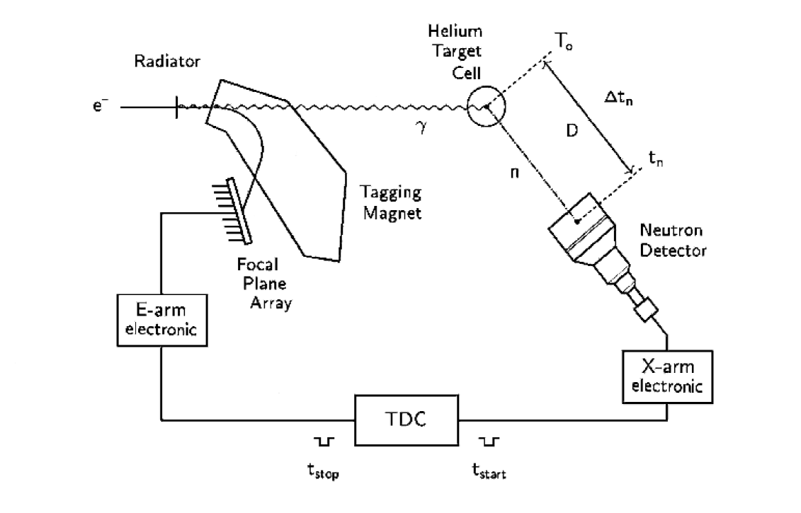
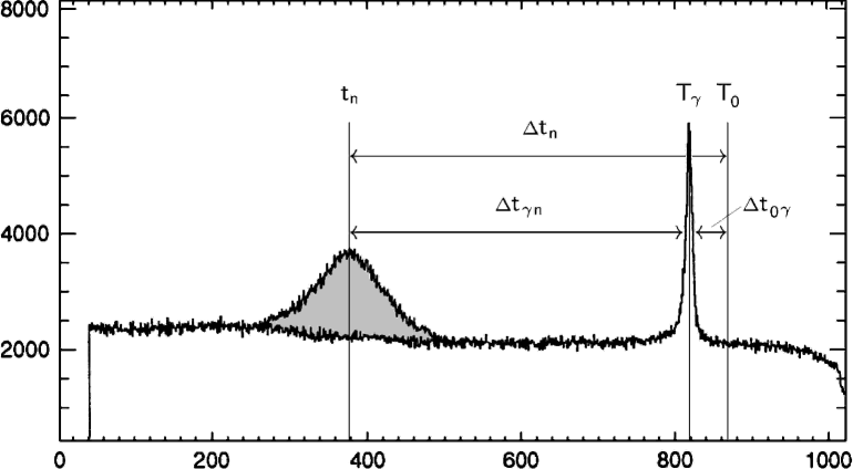
Events

TOF (TDC channels)

Figure 4: An illustration of the TOF technique. In the top panel, an overview of the TOF measurement is presented. A tagged photon knocks a neutron out of the ⁴He target which is then detected in the neutron-detector cell. This signal starts a TDC. The corresponding recoil electron is detected in the tagger focal plane, which results in a stop signal for the TDC. As a result, the TOF (and thus the neutron energy) is measured. In the bottom panel, a corresponding TOF spectrum is shown. Quasimonoenergetic neutrons are displayed as a gray bump superimposed on a random background. See text for further details.

II.4 Electronics and data acquisition

Figure 5: An overview of the experiment electronics. See text for further details.

An overview of the experiment electronics is presented in Figure 5. The analog signals from the liquid scintillators were symmetrically divided three ways and passed to a charge-to-digital converter (QDC), a PSD module, and a constant-fraction discriminator (CFD). The logical OR of the CFD signals, in anti-coincidence with the equivalent veto-detector output, formed a primary event trigger which was used to start the analog-to-digital circuitry.

The PSD modules were used to identify photons. When photons were identified, the logical outputs from the PSDs were used to abort the event processing and fast clear the QDCs and TDCs. When photons were not identified, the event was read out. The PSD thresholds were set conservatively to avoid the rejection of any neutrons, and as a result, a small fraction of the otherwise overwhelming number of background photon events “leaked” into the data set (see Figure 7).

No hardware coincidence was made between the neutron TOF spectrometers and the tagger focal-plane array, but coincidences were recorded in the TDCs attached to the 64 focal-plane counters. The neutron detectors made the common start. Focal-plane rates were recorded in the 64 free-running scalers also attached to the focal-plane counters. As the scalers were not inhibited during the data-acquisition dead time, proper normalization of the neutron yield required a livetime-efficiency correction. This correction was simply the ratio of the number of processed events (given by the sum of the scalers counting the number of read & clears and fast clears) to the number of potential triggers (which came from a free-running scaler counting the OR of the CFD signals). The system livetime was also estimated using two other methods which are described in detail in Ref. Nilsson (2003). The first method considered the interrupt rates of read & clears and fast clears together with their processing times and the duty factor of the beam. The second method considered the outputs of free-running and inhibited oscillators together with the duty factor of the beam. All three methods yielded the same results.

Figure 6 shows the distribution of livetime over the duration of the experiment, with each point in the Figure representing a single 1-hour run. As previously mentioned, the hardware PSD was purposely set rather “loose” so that no neutrons could accidentally be rejected. As a result, background photon events which made it into the data stream contributed overwhelmingly to the livetime of the system. As the neutron detectors were sensitive to even the smallest fluctuations in the electron beam, run-to-run variations in the livetime occurred for otherwise identical experiment configurations. Further, the background level was a strong function of angle, which also led to variations in the system livetime. The mean value was $\sim$50%.

Data acquisition and storage were handled using an in-house toolkit Ruijter (1995). Subsequent offline analysis was performed using the program acqu Annand (1993).

Figure 6: The livetime efficiency correction as a function of run number. Variations in the correction are due to variations in the event rate due to different electron-beam intensities and different neutron-detector angles. See text for further details.

III Analysis

III.1 Neutron-detector energy calibration

Gamma rays with energies ranging from 1.2 $<$ $E_{\gamma}$ $<$ 7.1 MeV from the sources ⁶⁰Co and ²³⁹PuBe were used to calibrate the energy deposited in the NE213A scintillators by measuring the pulse-height distributions from recoiling Compton electrons Annand et al. (1997). The method reported in Ref. Knox and Miller (1972) was used to determine the Compton edge position, but other prescriptions Flynn et al. (1964); King and Johnson (1984) did not produce a significantly different calibration. The calibration was necessary to determine the neutron-detection threshold (in MeV_ee or “MeV electron-equivalent”) which in turn was necessary to calculate the neutron-detection efficiency (see below). The non-linear response of NE213A to low-energy recoil protons was modeled using the empirical expression of Ref. Cecil et al. (1979). In general, the neutron-detection efficiency was very sensitive to the neutron pulse-height threshold, and thus a precise energy calibration of the NE213A scintillators was crucial.

III.2 Particle identification (PID)

As previously discussed, a PSD cut made using the trigger-processing electronics was used to reject photons at the hardware level, as the background photon flux was $\sim$10⁵ times greater than the neutron flux. More precise PID was performed offline using the recorded PS amplitude from the PSD module, plotted as a function of energy deposited in the NE213A scintillator (the “pulse height” or “PH” signal). Figure 7 shows the distinct separation between neutron and photon events which resulted.

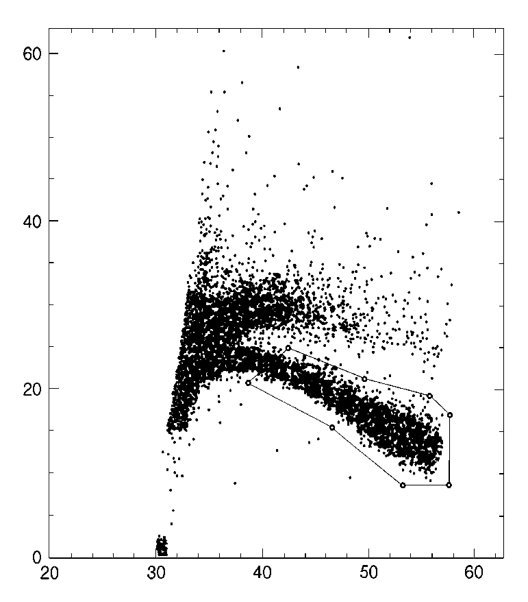
Pulse Shape (ADC channels)

Pulse Height (ADC channels)

Figure 7: A typical PID scatterplot for a single neutron-detector cell. Pulse shape (PS) was plotted versus pulse height (PH). Separation between neutrons and random photons is clearly demonstrated. The cut polygon which encircles the photon ridge was set very “loose” to ensure that no neutron events were discarded. Higher PH cuts were applied at a later stage of the data analysis. See text for further details.

III.3 Background removal

After the selection of candidate neutron events, the resulting data set for each neutron detector consisted of 64 TOF spectra containing both real coincidences with the tagger focal plane and a random background (see the top panel of Figure 8). The ratio of the number of prompt neutrons to random background was a strong function of photon energy, ranging from better than 1-to-1 at $E_{\gamma}$ $=$ 68.5 MeV to 1-to-10 at $E_{\gamma}$ $=$ 24.6 MeV.

Figure 8: A typical TOF spectrum measured at $\theta_{\rm LAB}$ $=$ 90 $\deg$ for $E_{\gamma}$ $=$ 29 MeV. Also shown in the top panel is the fitted function defined in Eq. (1). The prominent peak corresponds to neutron events. The same distribution, this time with the background removed and plotted as a function of neutron kinetic energy, is shown in the bottom panel. The vertical solid line is the fitted neutron-peak location (6.0 MeV), while the vertical dashed line is the anticipated neutron-peak location (6.1 MeV). See text for further details.

The removal of this random background proved to be a challenging exercise due to a periodic ripple in the time structure of the photon beam resulting from microstructure in the electron beam extracted from the pulse-stretcher ring Hoorebeke et al. (1993). This ripple may be clearly seen in the TOF spectrum shown in the top panel of Figure 8. Thus, the TOF spectra were fitted with a function of the form

$$Y(t)=A\cdot\exp~{}(B\cdot t)+C\cdot\sin(D\cdot t)+E\cdot\exp-(\frac{t-F}{\sqrt{2}~{}G})^{2}$$ (1)

to determine the random yield. A prompt Gaussian peak (coefficients E, F, and G) was superimposed upon a background which contained a sinusoidal term (coefficients C and D) to describe the ripple and an exponential term (coefficients A and B) which accounted for deadtime in the detector electronics and the single-hit TDCs which instrumented the tagger focal plane.

The bottom panel of Figure 8 shows the same distribution as in the top panel, but this time after the background had been removed and now plotted as a function of neutron kinetic energy. The background remaining after the subtraction is both flat as a function of energy and consistent with zero. The vertical solid line at 6.0 MeV is the neutron-peak location obtained from a Gaussian fit, while the vertical dashed line at 6.1 MeV is the expected location of the neutron peak based upon the tagger-determined photon energy and two-body ⁴He$(\gamma,n)$ kinematics. The 100 keV difference is less than the 300 keV photon-energy resolution which arises from the physical width of a single focal-plane counter.

The true number of neutrons was obtained after a “stolen-coincidence” correction Hornidge (2003) was applied to the neutron yield. Stolen coincidences occurred when an uncorrelated (random) recoil electron stopped the focal-plane TDCs prior to a (real) recoil electron correlated in time with a neutron event. A correction was applied to account for these events, which would otherwise be missed. The correction to the neutron yield was approximately 5% for the counting rates employed in the present experiment.

An identical analysis was performed on the empty-target data and demonstrated that there was no measurable contribution to the full-target spectra.

III.4 Cross section

The laboratory differential cross section for each photon-energy bin was extracted using

$$\frac{d\sigma}{d\Omega}(E_{\gamma},\theta)=\frac{Y(E_{\gamma},\theta)}{N_{\gamma}(E_{\gamma})\cdot\tau_{\rm He}\cdot\Delta\Omega(\theta)}$$ (2)

where $Y(E_{\gamma},\theta)$ was the true neutron yield corrected for electronic-livetime efficiency, neutron-detection efficiency, neutron-yield attenuation, and neutron inscattering; $N_{\gamma}(E_{\gamma})$ was the total number of photons corresponding to a given photon-energy bin corrected for focal-plane dead-time effects; $\tau_{\rm He}$ was the target thickness simulated using a geant3 model of the target cell and corrected for boiling effects and photon-flux attenuation; and $\Delta\Omega$ was the detector geometrical acceptance corrected for extended-target and extended-beam effects. The details of the corrections are discussed below. The resulting data are shown in Figure 11 and presented in Table 3. Figure 14 shows the angle-integrated cross-section data, which are presented in Table 6.

Figure 9: The neutron-attenuation, inscattering, and detection-efficiency corrections as a function of neutron kinetic energy. The estimated systematic uncertainties in these quantities are represented by the band at the base of each panel. See text for further details.

III.4.1 Neutron-yield attenuation

A neutron knocked out of the ⁴He nucleus into the acceptance of the neutron detectors had to first penetrate significant thicknesses of non-detector material before reaching the detector (see Figure 10). Thus, a correction for neutron-yield attenuation was necessary. Neutron absorption in the liquid ⁴He, the target cell, the target vacuum chamber, the air in the hall, the veto scintillator, and the liquid-scintillator canister was determined using a geant3-based gea model of the experiment setup. The correction was clearly largest at $T_{n}$ $<$ 10 MeV, and was dominated by the contribution of the veto detector, which was as large as $\sim$10%.

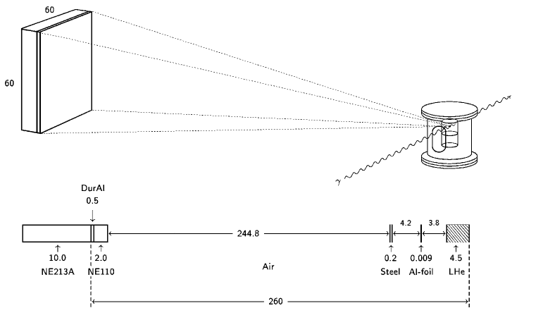
Figure 10: The relationship between the photon beam, the target cell, and the detector aperture is shown in the top panel. A cross-sectional view of the layers of matter between the target and the detector is shown in the bottom panel. All dimensions quoted are in cm. See text for further details.

III.4.2 Neutron inscattering

The geant3 model was also used to determine the neutron-inscattering correction to the data Nilsson (b). This effect arose from neutrons scattering in the materials between and around the target/detector system. The mass of material surrounding the detector was much greater than the mass of material which lay in the direct path between the target and the detector. Thus, the number of neutrons scattering into the detectors (which otherwise would have missed) exceeded the number of neutrons scattering out of the detectors (which otherwise would have hit). The Monte-Carlo model of the target and detectors was extended to include the neutron-detector lightguides, the shielding, and the support tables (recall Figure 3). The model was then embedded in a detailed mockup of the experiment hall, which included the concrete floor and ceiling (recall Figure 1). Appropriate TOF cuts which took into consideration the measured TOF resolution were employed to ensure that only neutrons of the correct energy were considered. The inscattering correction was a strong function of these cuts. As shown in the middle panel of Figure 9, this correction was also dependent upon neutron energy.

III.4.3 Neutron-detection efficiency

The neutron-detection efficiency was determined using the 1979 version of the stanton code Cecil et al. (1979). This code is based upon neutron cross-section data. The PH thresholds of the neutron-detector cells were set as low as possible in hardware to maximize the neutron-detection efficiency. However, in the offline analysis, the applied software threshold was varied above the hardware value in order to achieve the optimum compromise between neutron TOF signal-to-noise ratio and neutron-detection efficiency. The offline software threshold was used because the lower hardware voltage threshold had an associated uncertainty due to variations in the shape of the detected pulse. Ultimately, in all but the lowest $E_{\gamma}$ bins, the average PH threshold employed in the analysis was $\sim$2.0 MeV_ee, corresponding to a neutron energy of $\sim$4.5 MeV, and an average neutron-detection efficiency of $\sim$18% (see Figure 9).

Checks of the low-energy predictions made by stanton and geant3 were made by measuring the neutron-detection efficiency using a ²⁵²Cf fission-fragment source Karlsson (1997). A detailed description of the development and testing of geant3/stanton-based simulations of neutron detection is given in Ref. Reiter et al. (2006). This testing included the measurement of the well-known two-body deuteron photodisintegration cross section, which was also performed in previous MAX-lab $(\gamma,n)$ measurements Annand et al. (1993); Andersson et al. (1995). Unfortunately, time constraints prevented the installation of a deuterium target during the present experiment, but all MAX-lab $(\gamma,n)$ deuteron-photodisintegration tests of neutron-yield corrections have produced $(\gamma,n)$ cross sections which are entirely consistent with the generally accepted $(\gamma,p)$ values.

III.4.4 Number of photons

The procedure used for obtaining the number of photons incident upon the target is presented in detail in Ref. Adler et al. (1997). The incident photon flux for each photon-energy bin was determined by counting the number of recoil electrons in the tagger focal plane and multiplying the result by the measured tagging efficiency, which averaged $\sim$25%. Attenuation of the photon flux due to atomic processes within the target materials and the liquid helium itself Storm and Israel (1970) was also carefully investigated and found to be negligible. The 64 TOF spectra were summed in eight groups of eight tagger counters resulting in $\sim$2.5 MeV wide photon-energy bins, each accumulating $\sim$10¹² photons over the course of the measurement.

III.4.5 Geometrical acceptance

The geometrical acceptance of the neutron-detector cell was also determined using the geant3 simulation. In this manner, both the extended photon-beam profile and the resulting extended-target volume were considered. These extended-source effects resulted in a correction of approximately 1% to the $\sim$6 msr point-source acceptance of each cell.

III.4.6 Contamination of the two-body peak

The reaction thresholds for the $\gamma$ $+$ ⁴He $\rightarrow$ ³He + $n$ (2bbu) and $\gamma$ $+$ ⁴He $\rightarrow$ ²H $+$ $p$ $+$ $n$ (3bbu) are 20.57 and 26.06 MeV, respectively. Thus, if the neutron energy resolution is not sufficient, there may be some contamination of the 2bbu signal by 3bbu neutrons. This is particularly true for the higher photon-energy bins which correspond to higher neutron energies, since for a fixed target-to-detector flight path, the neutron-energy resolution degrades as the velocity increases.

An upper limit on the level of contamination of our results was determined using simulations ann performed within the root roo framework. These simulations were used to generate 2bbu and 3bbu neutrons according to the available kinematic phase space, and considered the extended beam, the target, and the detectors in the geometry of the experiment. With additional smearing to account for the electronic time-pickoff uncertainty, the measured widths of the observed 2bbu TOF peaks were reproduced well. Equal 2bbu and 3bbu total cross sections were assumed, and the number of 3bbu neutrons which impinged upon the 2bbu neutron-energy integration region was determined. The results are presented in Table 1.

Table 1: A summary of the contamination of the 2bbu yield by neutrons resulting from the 3bbu of ⁴He. The results represent an upper limit determined using equal 2bbu and 3bbu total cross sections. See text for further details.

$E_{\gamma}$	$<$contamination$>$
(MeV)	(%)
38.8	$<$0.1
40.6	$<$0.1
51.5	1.0
53.6	1.5
56.0	2.0
58.4	2.6
63.6	4.1
68.5	5.0

Cross-section data for the 3bbu reaction in the present energy range are sparce, but the available evidence Quaglioni et al. (2004) suggests that the 3bbu cross section is less than that for 2bbu. Thus, we believe that the results presented in Table 1 represent an upper limit on the contamination. We do not correct our data for this effect.

III.4.7 Systematic uncertainties

The systematic uncertainty in the measurement was dominated by the systematic uncertainty in the neutron-detection efficiency, which ranged from $\sim$5% for $E_{\gamma}$ $=$ 68.5 MeV to $\sim$26% for $E_{\gamma}$ $=$ 24.6 MeV. Other large sources of uncertainty were the neutron-inscattering correction ($\sim$9%), the neutron-yield attenuation correction ($\sim$6%), and the number of photons (a combination of the tagger focal-plane livetime and the tagging efficiency; $\sim$4%). A summary of the systematic uncertainties is presented in Table 2. The systematic uncertainties associated with each of the individual cross-section data points are presented in Tables 3 and 6. See also the discussion of the additional systematic uncertainties arising from the analysis of the angular distributions presented in Section IV.2, and the uncertainty bands shown in Figures 11 and 14.

Table 2: A summary of the correction factors applied to the cross-section data together with systematic uncertainties. In the case of the kinematic-dependent corrections, average values for the correction and the uncertainty are stated.

kinematic-dependent quantity	$<$value$>$	$<$uncertainty$>$
neutron-detection efficiency	0.20	8%
neutron-inscattering	1.25	9%
neutron-yield attenuation	0.85	6%
tagger focal-plane livetime	0.95	2%
neutron-detector livetime	0.50	1%
photon-beam attenuation	(see text)	$<$1%
scale quantity	value	uncertainty
tagging efficiency	0.25	3%
geometrical acceptance	(see text)	2%
target density	(see text)	2%
particle misidentification	(see text)	$<$1%

IV Results

IV.1 The calculations

In this Section, we compare our data to Recoil-Corrected Continuum Shell Model (RCCSM) calculations Halderson and Philpott (1981); Halderson (2004), a Resonating Group Method (RGM) calculation Wachter et al. (1988), and an Effective Interaction Hyperspherical Harmonic (EIHH) Expansion calculation Quaglioni et al. (2004). Note that the authors of the RCCSM and RGM calculations originally presented their results in the form of Legendre coefficients for the ³He$(n,\gamma)$ reaction expressed as a function of Center-of-Mass (c.m.) proton energy corresponding to the ³H$(p,\gamma)$ reaction, while the authors of the EIHH calculations present their results as a function of photon energy. These calculations consider only the two-fragment photodisintegration of ⁴He into the ($n+^{3}$He) final state.

The RCCSM calculations were performed using a continuum shell-model framework in the ($1p1h$) approximation where the transition-matrix elements of the M1 and the (spin-independent) M2 multipole operators vanished. Target-recoil corrections were applied. The effective nucleon-nucleon (NN) interaction included central, spin-orbit, and tensor components in addition to the Coulomb force. Perturbation theory was used to compute matrix elements for the multipoles. The multipole operators were calculated in the long-wavelength limit. After corrections applied for spurious c.m. excitations, these calculations were essentially equivalent to the multichannel microscopic RGM calculations described below. Note that the newer RCCSM calculation Halderson (2004) expanded the model space of the earlier calculation Halderson and Philpott (1981) to include more reaction channels and all $p$-shell nuclei.

The multichannel microscopic RGM calculations were performed using a semi-realistic NN force similar to the one detailed above. The variational principle was used to determine the scattering wave functions. Radiative processes were treated within the Born Approximation, and the electromagnetic transition operators were again taken in the long-wavelength limit. Angular momenta up to $L=2$ were allowed in the relative motion of the fragments. To the knowledge of the authors, further development of the RGM framework for photonuclear processes has ceased.

The EIHH calculation used a correlated hyperspherical expansion of basis states, with final-state interactions accounted for in a rigorous manner using the Lorentz Integral Transform Method (which circumvents the calculation of continuum wave functions).

IV.2 Angular distributions

Figure 11: c.m. angular distributions for the ⁴He$(\gamma,n)$ reaction from 23 $<$ E_γ $<$ 70 MeV. Error bars are the statistical uncertainties, while the systematic uncertainties are represented by the bands at the base of each panel. The solid lines are the fitted functions, while the dashed lines are the fitted functions extrapolated to zero at $\theta_{\rm c.m.}$ $=$ (0,180) $\deg$. See text for further details and Table 3 for numerical values.

The angular distributions measured at each photon energy were converted from the laboratory to the c.m. frame. In the two angular analyses we present below (and similar to analyses of complementary ⁴He$(\gamma,p)$ angular-distribution data Jones et al. (1991); cal ), we constrained our angular distributions to vanish at $\theta_{\rm c.m.}$ $=$ (0,180) $\deg$. We note that Weller et al. Weller et al. (1982) claim non-zero interfering E1 $S=1$ strength, which results in a non-vanishing angular distribution at $\theta_{\rm c.m.}$ $=$ (0,180) $\deg$. However, the present data do not have the precision and angular range necessary to investigate this small effect.

The systematic uncertainties in the angular distribution coefficients were estimated from the systematic uncertainties in the angular distributions (see Section III.4.7). Three extreme scenarios were considered, where the systematic uncertainty in the differential cross-section data would have a maximal effect upon the extracted angular-distribution coefficient. The first scenario involved shifting all the differential cross-section data points in an angular distribution either up or down in unison by their associated systematic uncertainty. The second scenario involved shifts of the same magnitude, but not in unison. Rather, they were made to either emphasize or de-emphasize the degree of forward/backward asymmetry in the angular distribution. The third scenario again involved shifts of the same magnitude, but this time to either emphasize or de-emphasize the peaking of the angular distribution at $\theta_{\rm c.m.}$ $\sim$ 90^∘. These three extreme sets of angular distributions were fitted as described in the sections below. The resulting systematic uncertainties were taken as the average spread in the value of the derived coefficients, and are displayed as error bands in Figures 12 and 13.

IV.2.1 The Transition-coefficient Approach

In the context of the Transition-coefficient Approach, the c.m. angular distributions were fitted using

$$\frac{d\sigma}{d\Omega}(\theta_{\rm c.m.})=\alpha~{}\left\{\sin^{2}(\theta_{\rm c.m.})\left[1+\beta\cos(\theta_{\rm c.m.})+\gamma\cos^{2}(\theta_{\rm c.m.})\right]+\delta+\epsilon\cos(\theta_{\rm c.m.})~{}\right\}.$$ (3)

This expansion assumes that the photon multipolarities are restricted to E1, E2, and M1, and that the nuclear matrix elements of the E-multipoles to final states with a channel spin of unity are negligible Jones et al. (1991). Under these assumptions, $\alpha$ arises from the incoherent sum of the E1, E2, and M1 multipoles, $\beta$ is due to the interference of the E1 and E2 multipoles, $\gamma$ results from the E2 multipole, $\delta$ arises from the M1 multipole, and $\epsilon$ is vanishingly small. As previously mentioned, in this analysis, the angular distributions were constrained to vanish at $\theta_{\rm c.m.}$ $=$ (0,180) $\deg$ – in this case, by forcing the $\delta$ and $\epsilon$ coefficients to be zero.

Figure 12 presents the $\alpha$, $\beta$, and $\gamma$ coefficients (filled circles) as a function of photon energy. The values are summarized in Table 4. Error bars are the statistical uncertainties, while the systematic uncertainties are represented by the bands at the base of each panel. Also shown are earlier RCCSM Halderson and Philpott (1981) and RGM Wachter et al. (1988) calculations. Angular distributions were not published in Refs. Halderson (2004) (newer RCCSM) or Quaglioni et al. (2004) (EIHH).

Figure 12: The $\alpha$, $\beta$, and $\gamma$ coefficients: present data – filled circles; earlier RCCSM calculations Halderson and Philpott (1981) – solid lines; RGM calculation Wachter et al. (1988) – dashed line. Error bars are the statistical uncertainties, while the systematic uncertainties are represented by the bands at the base of each panel. See text for further details.

As shown, the data basically follow the trends predicted by the calculations. At the lower photon energies where the E1 multipole is completely dominant, the $\alpha$-coefficient data have a clear resonant structure peaking at $E_{\gamma}$ $\sim$ 28 MeV. The earlier RCCSM calculation tends to overestimate the data, but also shows resonant structure peaking at $E_{\gamma}$ $\sim$ 25 MeV. The energy dependence of the $\beta$-coefficient data is reasonably consistent with both the earlier RCCSM and the RGM predictions, given the systematic uncertainties for $E_{\gamma}$ $<$ 26 MeV. Similarly, there is no significant disagreement between the present $\gamma$-coefficient data and the earlier RCCSM calculation when uncertainties are considered. At higher photon energies, E2 strength is expected to become more important. Unfortunately, the calculations do not cover the range of the higher-energy data. That said, these data do appear to be consistent with the energy-extrapolated trends of both the lower-energy data and the calculations.

IV.2.2 The Legendre Approach

In the context of the Legendre Approach, the c.m. angular distributions were fitted using

$$\frac{d\sigma}{d\Omega}(\theta_{\rm c.m.})=A_{0}\left[1+\sum_{n=1}^{4}a_{n}P_{n}(\cos(\theta_{\rm c.m.}))\right].$$ (4)

The angular distributions were constrained to vanish at $\theta_{\rm c.m.}$ $=$ (0,180) $\deg$ by enforcing the constraints $a_{1}=-a_{3}$ and $1+a_{2}+a_{4}=0$ (equivalent to the $\delta=\epsilon=0$ constraints used in the Transition-coefficient Approach).

Figure 13 presents the $A_{0}$ and $a_{1}$–$a_{4}$ coefficients (filled circles). Values are summarized in Table 5. Error bars are the statistical uncertainties, while the systematic uncertainties are represented by the bands at the base of each panel. Also shown are earlier RCCSM Halderson and Philpott (1981) and RGM Wachter et al. (1988) calculations for the ³He$(n,\gamma)$ reaction. In keeping with the convention chosen by the authors of these theoretical works, our data and their calculations have been plotted as a function of c.m. proton energy for the ³H$(p,\gamma)$ reaction.

As shown again, the data largely reproduce the trends predicted by the calculations. At lower energies, the E1 multipole is completely dominant and the $A_{0}$ coefficient has a clear resonant structure peaking at $E_{p}$ $\sim$ 7 MeV. The earlier RCCSM calculation tends to overestimate these data, but also has the resonant structure peaking at $E_{p}$ $\sim$ 6 MeV. The energy dependence of the $a_{1}=-a_{3}$ data is reasonably consistent with both the earlier RCCSM and RGM predictions, given the systematic uncertainties for $E_{p}$ $<$ 8 MeV. Similarly, there is no significant disagreement between the present $a_{2}=-(1+a_{4})$ data and the calculations. Finally, while the calculations again do not cover the range of the higher-energy data where the E2 strength is expected to become more important, these data do appear to be consistent with the energy-dependent trends of both the lower-energy data and the calculations.

Figure 13: The Legendre coefficients: present data – filled circles; earlier RCCSM calculations Halderson and Philpott (1981) – solid lines; RGM calculation Wachter et al. (1988) – dashed line. Error bars are the statistical uncertainties, while the systematic uncertainties are represented by the bands at the base of each panel. See text for further details.

IV.3 Angle-integrated cross section

Figure 14 presents the angle-integrated cross-section data (filled circles). Also shown are the CBD evaluation Calarco et al. (1983), data from a ³He$(n,\gamma)$ measurement Komar et al. (1993), data from ⁴He$(\gamma,^{3}$He$)$ active-target measurements Shima et al. (2001, 2005), the newer RCCSM calculation Halderson (2004), and the EIHH calculation Quaglioni et al. (2004). Note that both calculations employ the semi-realistic MTI-III potential Malfliet and Tjon (1969). Error bars show the statistical uncertainties, while the systematic uncertainties are represented by the bands at the base of the panel. For clarity, the systematic uncertainties in the data from Refs. Shima et al. (2005, 2001) have been centered at $-$0.1 and $-$0.25, respectively. Also for clarity, the small uncertainty in the EIHH calculation for the photon-energy region between 2bbu threshold at $E_{\gamma}$ $=$ 20.6 MeV and 3bbu threshold at $E_{\gamma}$ $=$ 26.1 MeV discussed in Ref. Quaglioni et al. (2004) is not shown here.

Figure 14: The angle-integrated ⁴He$(\gamma,n)$ cross section: present data – filled circles; CBD evaluation Calarco et al. (1983) – hatched band; RCCSM calculation Halderson (2004) – dashed-dotted line; and EIHH calculation Quaglioni et al. (2004) – solid line. Error bars are the statistical uncertainties, while the systematic uncertainties associated with each of the data sets are represented by the bands at the base of the panel. See text for further details.

The present ⁴He$(\gamma,n)$ angle-integrated cross-section data has a clear resonant structure which peaks at $E_{\gamma}$ $\sim$ 28 MeV. On average, these data are approximately 7% larger than those which result from simply scaling our projected $\theta_{\rm c.m.}$ $=$ 90 $\deg$ results by $8\pi/3$. Although data are lacking for 42 $<$ $E_{\gamma}$ $<$ 50 MeV, there is no apparent discontinuity in this region. Furthermore, the present data extrapolate smoothly to the lower-energy data of Ref. Komar et al. (1993). Conversely, the data of Refs. Shima et al. (2001, 2005) below 25 MeV are at odds with all other data, the calculations, and the CBD evaluation, although it is in good agreement with the present experiment near 30 MeV. Both the RCCSM and EIHH calculations are in good agreement with the present data and those of Ref. Komar et al. (1993) up to the resonant peak at $E_{\gamma}$ $\sim$ 28 MeV. At higher energies, both calculations tend to overpredict the data. Nevertheless, the EIHH calculation follows the general shape of the excitation function up to $E_{\gamma}$ $\sim$ 70 MeV reasonably well. Development of the EIHH formalism continues Gazit et al. (2006); Barnea et al. so that the total photoabsorption may now be calculated using the Argonne V18 NN potential in conjunction with the Urbana IX 3N potential, and we anticipate new predictions for the partial two-body photodisintegration channels in the near future.

V Summary and conclusions

In summary, $\frac{d\sigma}{d\Omega}(E_{\gamma},\theta)$ for the ⁴He$(\gamma,n)$ reaction have been measured with tagged photons and compared to other available measurements and calculations. The energy dependence of the transition coefficients $\alpha$, $\beta$, and $\gamma$ as well as the Legendre coefficients $A_{0}$, $a_{1}$, and $a_{2}$ extracted from the angular distributions agrees reasonably well with trends predicted by earlier RCCSM Halderson and Philpott (1981) and RGM Wachter et al. (1988) calculations. The marked resonant behavior of the present angle-integrated cross section, peaking at $E_{\gamma}$ $\sim$ 28 MeV, is in good agreement with newer RCCSM Halderson (2004) and EIHH Quaglioni et al. (2004) calculations as well as capture data Komar et al. (1993) which extend close to the $(\gamma,n)$ threshold. This behavior disagrees with an evaluation of $(\gamma,n)$ data Calarco et al. (1983) made in 1983, and recent active-target data Shima et al. (2001, 2005).

Appendix A Data tables

A.1 Differential cross-section data

A summary of the differential cross-section data is presented in Table 3.

Table 3: The differential cross-section data (mb/sr) for the ⁴He$(\gamma,n)$ reaction shown in Fig. 11. The first uncertainty is statistical and the second uncertainty is systematic.

$\theta_{\rm c.m.}$	d$\sigma$/d$\Omega_{\rm c.m.}$	$\theta_{\rm c.m.}$	d$\sigma$/d$\Omega_{\rm c.m.}$
($\deg$)	(mb/sr)	($\deg$)	(mb/sr)
$E_{\gamma}$ $=$ 24.6 MeV		$E_{\gamma}$ $=$ 26.7 MeV
		47.9	0.091 $\pm$ 0.009 $\pm$ 0.015
64.1	0.124 $\pm$ 0.020 $\pm$ 0.023	63.6	0.114 $\pm$ 0.007 $\pm$ 0.019
79.6	0.154 $\pm$ 0.014 $\pm$ 0.034	79.0	0.152 $\pm$ 0.007 $\pm$ 0.025
94.8	0.145 $\pm$ 0.010 $\pm$ 0.040	94.2	0.197 $\pm$ 0.008 $\pm$ 0.036
109.6	0.167 $\pm$ 0.018 $\pm$ 0.049	109.0	0.202 $\pm$ 0.008 $\pm$ 0.039
124.1	0.087 $\pm$ 0.010 $\pm$ 0.017	123.6	0.166 $\pm$ 0.009 $\pm$ 0.030
138.4	0.111 $\pm$ 0.018 $\pm$ 0.038	137.9	0.130 $\pm$ 0.008 $\pm$ 0.025
$E_{\gamma}$ $=$ 28.9 MeV		$E_{\gamma}$ $=$ 31.1 MeV
47.7	0.079 $\pm$ 0.006 $\pm$ 0.010	47.6	0.065 $\pm$ 0.005 $\pm$ 0.008
63.4	0.108 $\pm$ 0.005 $\pm$ 0.014	63.2	0.089 $\pm$ 0.004 $\pm$ 0.010
78.7	0.145 $\pm$ 0.005 $\pm$ 0.020	78.6	0.105 $\pm$ 0.004 $\pm$ 0.012
93.9	0.144 $\pm$ 0.006 $\pm$ 0.020	93.7	0.106 $\pm$ 0.004 $\pm$ 0.013
108.7	0.166 $\pm$ 0.006 $\pm$ 0.025	108.6	0.123 $\pm$ 0.004 $\pm$ 0.015
123.4	0.144 $\pm$ 0.006 $\pm$ 0.021	123.2	0.115 $\pm$ 0.005 $\pm$ 0.014
137.7	0.109 $\pm$ 0.006 $\pm$ 0.017	137.6	0.082 $\pm$ 0.004 $\pm$ 0.010
$E_{\gamma}$ $=$ 34.6 MeV		$E_{\gamma}$ $=$ 36.4 MeV
47.5	0.045 $\pm$ 0.005 $\pm$ 0.005	47.5	0.040 $\pm$ 0.004 $\pm$ 0.005
63.1	0.061 $\pm$ 0.004 $\pm$ 0.007	63.0	0.068 $\pm$ 0.004 $\pm$ 0.008
78.5	0.093 $\pm$ 0.004 $\pm$ 0.011	78.4	0.093 $\pm$ 0.005 $\pm$ 0.011
93.6	0.089 $\pm$ 0.004 $\pm$ 0.010	93.5	0.079 $\pm$ 0.004 $\pm$ 0.009
108.5	0.094 $\pm$ 0.004 $\pm$ 0.011	108.5	0.067 $\pm$ 0.003 $\pm$ 0.008
123.1	0.075 $\pm$ 0.004 $\pm$ 0.009	123.1	0.075 $\pm$ 0.004 $\pm$ 0.009
137.5	0.051 $\pm$ 0.004 $\pm$ 0.006	137.5	0.052 $\pm$ 0.004 $\pm$ 0.006
$E_{\gamma}$ $=$ 38.8 MeV		$E_{\gamma}$ $=$ 40.7 MeV
47.5	0.033 $\pm$ 0.004 $\pm$ 0.004	47.5	0.037 $\pm$ 0.004 $\pm$ 0.004
63.1	0.059 $\pm$ 0.004 $\pm$ 0.007	63.0	0.047 $\pm$ 0.004 $\pm$ 0.006
78.4	0.071 $\pm$ 0.005 $\pm$ 0.008	78.4	0.064 $\pm$ 0.004 $\pm$ 0.007
93.5	0.073 $\pm$ 0.004 $\pm$ 0.009	93.5	0.057 $\pm$ 0.004 $\pm$ 0.007
108.4	0.074 $\pm$ 0.004 $\pm$ 0.009	108.4	0.061 $\pm$ 0.003 $\pm$ 0.007
123.0	0.058 $\pm$ 0.004 $\pm$ 0.007	123.0	0.047 $\pm$ 0.003 $\pm$ 0.006
137.5	0.041 $\pm$ 0.004 $\pm$ 0.005	137.5	0.035 $\pm$ 0.003 $\pm$ 0.004
$E_{\gamma}$ $=$ 51.4 MeV		$E_{\gamma}$ $=$ 53.6 MeV
31.0	0.013 $\pm$ 0.004 $\pm$ 0.001	31.0	0.011 $\pm$ 0.003 $\pm$ 0.001
45.9	0.027 $\pm$ 0.005 $\pm$ 0.003	45.9	0.022 $\pm$ 0.005 $\pm$ 0.002
62.1	0.031 $\pm$ 0.004 $\pm$ 0.003	62.1	0.037 $\pm$ 0.004 $\pm$ 0.004
77.0	0.035 $\pm$ 0.005 $\pm$ 0.003	77.0	0.029 $\pm$ 0.004 $\pm$ 0.003
92.1	0.033 $\pm$ 0.006 $\pm$ 0.005	92.1	0.026 $\pm$ 0.005 $\pm$ 0.004
108.3	0.035 $\pm$ 0.006 $\pm$ 0.003	108.3	0.029 $\pm$ 0.005 $\pm$ 0.003
123.1	0.024 $\pm$ 0.004 $\pm$ 0.002	123.1	0.023 $\pm$ 0.003 $\pm$ 0.002
$E_{\gamma}$ $=$ 56.0 MeV		$E_{\gamma}$ $=$ 58.4 MeV
31.0	0.012 $\pm$ 0.004 $\pm$ 0.001	31.0	0.014 $\pm$ 0.003 $\pm$ 0.001
45.9	0.019 $\pm$ 0.004 $\pm$ 0.002	45.9	0.019 $\pm$ 0.004 $\pm$ 0.002
62.1	0.035 $\pm$ 0.004 $\pm$ 0.003	62.1	0.026 $\pm$ 0.004 $\pm$ 0.002
77.0	0.034 $\pm$ 0.004 $\pm$ 0.003	77.0	0.030 $\pm$ 0.004 $\pm$ 0.002
92.1	0.030 $\pm$ 0.005 $\pm$ 0.004	92.1	0.026 $\pm$ 0.005 $\pm$ 0.004
108.3	0.022 $\pm$ 0.006 $\pm$ 0.002	108.3	0.022 $\pm$ 0.005 $\pm$ 0.002
123.1	0.022 $\pm$ 0.003 $\pm$ 0.002	123.2	0.017 $\pm$ 0.003 $\pm$ 0.003
$E_{\gamma}$ $=$ 63.6 MeV		$E_{\gamma}$ $=$ 68.5 MeV
31.0	0.009 $\pm$ 0.003 $\pm$ 0.001	31.0	0.008 $\pm$ 0.002 $\pm$ 0.001
45.9	0.012 $\pm$ 0.004 $\pm$ 0.001	45.9	0.014 $\pm$ 0.003 $\pm$ 0.001
62.1	0.020 $\pm$ 0.003 $\pm$ 0.002	62.1	0.020 $\pm$ 0.002 $\pm$ 0.002
77.0	0.015 $\pm$ 0.003 $\pm$ 0.001	77.0	0.022 $\pm$ 0.002 $\pm$ 0.002
92.1	0.017 $\pm$ 0.004 $\pm$ 0.002	92.1	0.018 $\pm$ 0.003 $\pm$ 0.003
108.3	0.019 $\pm$ 0.004 $\pm$ 0.002	108.3	0.014 $\pm$ 0.003 $\pm$ 0.002
123.2	0.013 $\pm$ 0.004 $\pm$ 0.001	123.3	0.008 $\pm$ 0.002 $\pm$ 0.001

A.2 Angular-distribution coefficients

A summary of the angular-distribution coefficients is presented in Tables 4 and 5.

Table 4: A summary of the coefficients $\alpha$, $\beta$, and $\gamma$ extracted from the data. The first uncertainty is statistical and the second uncertainty is systematic. See also Figure 12.

$E_{\gamma}$	$\alpha$	$\beta$	$\gamma$
(MeV)	(mb/sr)
24.6	0.151 $\pm$ 0.009 $\pm$ 0.035	0.081 $\pm$ 0.193 $\pm$ 0.418	0.186 $\pm$ 0.440 $\pm$ 1.093
26.7	0.180 $\pm$ 0.005 $\pm$ 0.026	$-$0.545 $\pm$ 0.055 $\pm$ 0.158	0.341 $\pm$ 0.149 $\pm$ 0.421
28.9	0.151 $\pm$ 0.004 $\pm$ 0.017	$-$0.414 $\pm$ 0.048 $\pm$ 0.085	0.533 $\pm$ 0.134 $\pm$ 0.335
31.1	0.111 $\pm$ 0.003 $\pm$ 0.009	$-$0.380 $\pm$ 0.050 $\pm$ 0.121	0.785 $\pm$ 0.143 $\pm$ 0.178
34.6	0.094 $\pm$ 0.003 $\pm$ 0.009	$-$0.249 $\pm$ 0.061 $\pm$ 0.141	0.004 $\pm$ 0.148 $\pm$ 0.246
36.4	0.080 $\pm$ 0.003 $\pm$ 0.007	$-$0.104 $\pm$ 0.060 $\pm$ 0.224	0.419 $\pm$ 0.166 $\pm$ 0.280
38.8	0.076 $\pm$ 0.003 $\pm$ 0.003	$-$0.183 $\pm$ 0.071 $\pm$ 0.153	0.021 $\pm$ 0.179 $\pm$ 0.260
40.7	0.061 $\pm$ 0.003 $\pm$ 0.003	$-$0.075 $\pm$ 0.077 $\pm$ 0.185	0.287 $\pm$ 0.206 $\pm$ 0.215
51.4	0.034 $\pm$ 0.004 $\pm$ 0.003	0.186 $\pm$ 0.176 $\pm$ 0.117	0.450 $\pm$ 0.516 $\pm$ 0.344
53.6	0.030 $\pm$ 0.003 $\pm$ 0.003	0.253 $\pm$ 0.165 $\pm$ 0.136	0.672 $\pm$ 0.494 $\pm$ 0.262
56.0	0.032 $\pm$ 0.003 $\pm$ 0.003	0.319 $\pm$ 0.157 $\pm$ 0.103	0.254 $\pm$ 0.443 $\pm$ 0.239
58.4	0.027 $\pm$ 0.003 $\pm$ 0.002	0.423 $\pm$ 0.185 $\pm$ 0.141	0.443 $\pm$ 0.526 $\pm$ 0.289
63.6	0.017 $\pm$ 0.003 $\pm$ 0.002	0.146 $\pm$ 0.308 $\pm$ 0.156	1.091 $\pm$ 0.893 $\pm$ 0.336
68.5	0.019 $\pm$ 0.002 $\pm$ 0.002	0.706 $\pm$ 0.170 $\pm$ 0.124	$-$0.151 $\pm$ 0.398 $\pm$ 0.250

Table 5: A summary of the Legendre coefficients extracted from the data. The first uncertainty is statistical and the second uncertainty is systematic. See also Figure 13.

$E_{\gamma}$	$A_{0}$	$a_{1}$	$a_{2}$	$a_{3}$	$a_{4}$
(MeV)	(mb/sr)			($=-a_{1}$)	($=-(1+a_{2})$)
24.6	0.105 $\pm$ 0.007 $\pm$ 0.012	0.041 $\pm$ 0.108 $\pm$ 0.225	$-$0.936 $\pm$ 0.134 $\pm$ 0.331	$-$0.041 $\pm$ 0.108 $\pm$ 0.225	$-$0.064 $\pm$ 0.134 $\pm$ 0.331
26.7	0.129 $\pm$ 0.003 $\pm$ 0.010	$-$0.311 $\pm$ 0.032 $\pm$ 0.103	$-$0.884 $\pm$ 0.044 $\pm$ 0.123	0.311 $\pm$ 0.032 $\pm$ 0.103	$-$0.116 $\pm$ 0.044 $\pm$ 0.123
28.9	0.111 $\pm$ 0.002 $\pm$ 0.007	$-$0.229 $\pm$ 0.027 $\pm$ 0.079	$-$0.830 $\pm$ 0.037 $\pm$ 0.095	0.229 $\pm$ 0.027 $\pm$ 0.079	$-$0.170 $\pm$ 0.037 $\pm$ 0.095
31.1	0.086 $\pm$ 0.001 $\pm$ 0.006	$-$0.200 $\pm$ 0.026 $\pm$ 0.088	$-$0.762 $\pm$ 0.036 $\pm$ 0.054	0.200 $\pm$ 0.026 $\pm$ 0.088	$-$0.238 $\pm$ 0.036 $\pm$ 0.054
34.6	0.062 $\pm$ 0.002 $\pm$ 0.003	$-$0.155 $\pm$ 0.037 $\pm$ 0.061	$-$0.992 $\pm$ 0.050 $\pm$ 0.085	0.155 $\pm$ 0.037 $\pm$ 0.061	$-$0.008 $\pm$ 0.050 $\pm$ 0.085
36.4	0.058 $\pm$ 0.001 $\pm$ 0.003	$-$0.062 $\pm$ 0.034 $\pm$ 0.062	$-$0.864 $\pm$ 0.047 $\pm$ 0.081	0.062 $\pm$ 0.034 $\pm$ 0.062	$-$0.136 $\pm$ 0.047 $\pm$ 0.081
38.8	0.051 $\pm$ 0.001 $\pm$ 0.002	$-$0.115 $\pm$ 0.042 $\pm$ 0.063	$-$0.987 $\pm$ 0.059 $\pm$ 0.088	0.115 $\pm$ 0.042 $\pm$ 0.063	$-$0.013 $\pm$ 0.059 $\pm$ 0.088
40.7	0.043 $\pm$ 0.001 $\pm$ 0.002	$-$0.048 $\pm$ 0.044 $\pm$ 0.081	$-$0.902 $\pm$ 0.061 $\pm$ 0.073	0.048 $\pm$ 0.044 $\pm$ 0.081	$-$0.098 $\pm$ 0.061 $\pm$ 0.073
51.4	0.025 $\pm$ 0.002 $\pm$ 0.001	0.097 $\pm$ 0.097 $\pm$ 0.067	$-$0.854 $\pm$ 0.138 $\pm$ 0.073	$-$0.097 $\pm$ 0.097 $\pm$ 0.067	$-$0.146 $\pm$ 0.138 $\pm$ 0.073
53.6	0.023 $\pm$ 0.001 $\pm$ 0.001	0.130 $\pm$ 0.087 $\pm$ 0.075	$-$0.794 $\pm$ 0.121 $\pm$ 0.064	$-$0.130 $\pm$ 0.087 $\pm$ 0.075	$-$0.206 $\pm$ 0.121 $\pm$ 0.064
56.0	0.023 $\pm$ 0.001 $\pm$ 0.001	0.176 $\pm$ 0.089 $\pm$ 0.064	$-$0.914 $\pm$ 0.128 $\pm$ 0.064	$-$0.176 $\pm$ 0.089 $\pm$ 0.064	$-$0.086 $\pm$ 0.128 $\pm$ 0.064
58.4	0.020 $\pm$ 0.001 $\pm$ 0.001	0.227 $\pm$ 0.102 $\pm$ 0.083	$-$0.856 $\pm$ 0.139 $\pm$ 0.069	$-$0.227 $\pm$ 0.102 $\pm$ 0.083	$-$0.144 $\pm$ 0.139 $\pm$ 0.069
63.6	0.014 $\pm$ 0.001 $\pm$ 0.001	0.070 $\pm$ 0.151 $\pm$ 0.077	$-$0.687 $\pm$ 0.186 $\pm$ 0.059	$-$0.070 $\pm$ 0.151 $\pm$ 0.077	$-$0.313 $\pm$ 0.186 $\pm$ 0.059
68.5	0.013 $\pm$ 0.001 $\pm$ 0.001	0.422 $\pm$ 0.103 $\pm$ 0.086	$-$1.042 $\pm$ 0.135 $\pm$ 0.073	$-$0.422 $\pm$ 0.103 $\pm$ 0.086	0.042 $\pm$ 0.135 $\pm$ 0.073

A.3 Angle-integrated cross-section data

A summary of the angle-integrated cross-section data is presented in Table 6.

Table 6: A summary of the angle-integrated cross-section data. The first uncertainty is statistical and the second uncertainty is systematic. See also Figure 14.

$E_{\gamma}$	$\sigma$
(MeV)	(mb)
24.6	1.310 $\pm$ 0.134 $\pm$ 0.289
26.7	1.610 $\pm$ 0.064 $\pm$ 0.287
28.8	1.397 $\pm$ 0.049 $\pm$ 0.198
31.1	1.072 $\pm$ 0.038 $\pm$ 0.131
34.6	0.786 $\pm$ 0.034 $\pm$ 0.092
36.4	0.729 $\pm$ 0.035 $\pm$ 0.085
38.8	0.635 $\pm$ 0.033 $\pm$ 0.075
40.6	0.542 $\pm$ 0.031 $\pm$ 0.064
51.4	0.314 $\pm$ 0.046 $\pm$ 0.003
53.6	0.287 $\pm$ 0.039 $\pm$ 0.003
56.0	0.284 $\pm$ 0.038 $\pm$ 0.003
58.4	0.243 $\pm$ 0.037 $\pm$ 0.003
63.6	0.170 $\pm$ 0.036 $\pm$ 0.002
68.5	0.158 $\pm$ 0.019 $\pm$ 0.002

References

- Calarco et al. (1983) J. R. Calarco, B. L. Berman, and T. W. Donnelly, Phys. Rev. C. 27, 1866 (1983), and the references therein.
- Quaglioni et al. (2004) S. Quaglioni, W. Leidemann, G. Orlandini, N. Barnea, and V. D. Efros, Phys. Rev. C. 69, 044002 (2004), and the references therein.
- Shima et al. (2005) T. Shima, S. Naito, Y. Nagai, T. Baba, K. Tamura, T. Takahashi, T. Kii, H. Ohgaki, and H. Toyokawa, Phys. Rev. C. 72, 044004 (2005).
- Komar et al. (1993) R. J. Komar, H. B. Mak, J. R. Leslie, H. C. Evans, E. Bonvin, E. D. Earle, and T. K. Alexander, Phys. Rev. C. 48, 2375 (1993), and the references therein.
- Shima et al. (2001) T. Shima, Y. Nagai, T. Baba, T. Takahashi, T. Kii, H. Ohgaki, and H. Toyokawa, Nucl. Phys. A687, 127c (2001).
- Halderson and Philpott (1981) D. Halderson and R. J. Philpott, Nucl. Phys. A359, 365 (1981), and the references therein; the calculation shown for in the top panel of Fig. 12 was provided via private communication.
- Halderson (2004) D. Halderson, Phys. Rev. C. 70, 034607 (2004), and the references therein.
- Wachter et al. (1988) B. Wachter, T. Mertelmeier, and H. M. Hofmann, Phys. Rev. C. 38, 1139 (1988), and the references therein.
- Nilsson (2003) B. Nilsson, Ph.D. thesis, University of Lund, Sweden (2003), eprint http://www.maxlab.lu.se/kfoto/publications/nilsson.pdf.
- Sims et al. (1998) D. A. Sims et al., Phys. Lett. B442, 43 (1998).
- Nilsson et al. (2005) B. Nilsson et al., Phys. Lett. B626, 65 (2005).
- Adler et al. (1997) J. O. Adler et al., Nucl. Instrum. Methods Phys. Res. Sect. A 388, 17 (1997).
- (13) eprint http://www.maxlab.lu.se/.
- Adler et al. (1990) J. O. Adler et al., Nucl. Instrum. Methods Phys. Res. Sect. A 294, 15 (1990).
- Tate and Sadler (1983) M. W. Tate and M. E. Sadler, Nucl. Instrum. Methods 204, 295 (1983).
- Nilsson (a) B. Nilsson, eprint to be submitted to Nucl. Instrum. Methods Phys. Res. Sect. A in 2006.
- Annand et al. (1997) J. R. M. Annand, B. E. Andersson, I. Akkurt, and B. Nilsson, Nucl. Instrum. Methods Phys. Res. Sect. A 400, 344 (1997).
- Annand (1987) J. R. M. Annand, Nucl. Instrum. Methods Phys. Res. Sect. A 262, 371 (1987).
- Ruijter (1995) H. Ruijter, Ph.D. thesis, University of Lund, Sweden (1995), eprint http://www.maxlab.lu.se/kfoto/publications/ruijter.pdf.
- Annand (1993) J. R. M. Annand, Kelvin Laboratory Data Acquisition System for Nuclear Physics, University of Glasgow, UK (1993).
- Knox and Miller (1972) H. H. Knox and T. G. Miller, Nucl. Instrum. Methods 101, 519 (1972).
- Flynn et al. (1964) K. F. Flynn, L. E. Glendenin, E. P. Steinberg, and P. M. Wright, Nucl. Instrum. Methods 27, 13 (1964).
- King and Johnson (1984) K. J. King and T. L. Johnson, Nucl. Instrum. Methods 227, 257 (1984).
- Cecil et al. (1979) R. A. Cecil, B. D. Anderson, and R. Madey, Nucl. Instrum. Methods 161, 439 (1979).
- Hoorebeke et al. (1993) L. V. Hoorebeke, D. Ryckbosch, C. V. den Abeele, R. V. de Vyver, and J. Dias, Nucl. Instrum. Methods Phys. Res. Sect. A 326, 608 (1993).
- Hornidge (2003) D. Hornidge, Ph.D. thesis, University of Saskatchewan, Canada (2003), eprint see also http://www.mta.ca/~dhornidg/phd_thesis.pdf.
- (27) eprint http://wwwasd.web.cern.ch/wwwasd/geant/.
- Nilsson (b) B. Nilsson, eprint to be submitted to Nucl. Instrum. Methods Phys. Res. Sect. A in 2006.
- Karlsson (1997) M. Karlsson, Master’s thesis, University of Lund, Sweden (1997), eprint see also http://www.maxlab.lu.se/kfoto/publications/karlsson_xjobb.pdf.
- Reiter et al. (2006) A. Reiter et al., Nucl. Instrum. Methods Phys. Res. Sect. A 565, 753 (2006).
- Annand et al. (1993) J. R. M. Annand et al., Phys. Rev. Lett. 71, 2703 (1993).
- Andersson et al. (1995) B. E. Andersson et al., Phys. Rev. C. 51, 2553 (1995).
- Storm and Israel (1970) E. Storm and H. I. Israel, Nucl. Data Tables A7, 565 (1970).
- (34) eprint http://nuclear.gla.ac.uk/~jrma/MAX-lab/HeSim.pdf.
- (35) eprint http://root.cern.ch/.
- Jones et al. (1991) R. T. Jones, D. A. Jenkins, P. T. Debevec, P. D. Harty, and J. E. Knott, Phys. Rev. C. 43, 2052 (1991), and the references therein.
- (37) eprint J. Calarco, private communication.
- Weller et al. (1982) H. R. Weller, N. R. Roberson, G. Mitev, L. Ward, and D. R. Tilley, Phys. Rev. C. 25, 2111 (1982).
- Malfliet and Tjon (1969) R. A. Malfliet and J. Tjon, Nucl. Phys. A127, 161 (1969).
- Gazit et al. (2006) D. Gazit, S. Bacca, N. Barnea, W. Leidemann, and G. Orlandini, Phys. Rev. Lett. 96, 112301 (2006).
- (41) N. Barnea, W. Leidemann, and G. Orlandini, eprint nucl-th/0607011.